Energy-superconvergent Runge-Kutta Time Discretizations
Abstract
In this paper, we investigate the energy accuracy of explicit Runge-Kutta (RK) time discretization for antisymmetric autonomous linear systems and present a framework for constructing RK methods with an order of energy accuracy much greater than the number of stages. For an -stage, th-order RK method, we show that the energy accuracy can achieve superconvergence with an order up to if is even. Several energy-superconvergent methods, including five- to seven-stage fourth-order methods with energy accuracy up to the eleventh order, together with their strong stability criteria, are derived. The proposed methods are examined using several applications, including second-order ordinary differential equations for harmonic oscillators, linear integro-differential equations for peridynamics, and one-dimensional Maxwell’s equations of electrodynamics.
Keywords: Runge-Kutta methods; Superconvergence; Hamiltonian; Energy accuracy; Peridynamics; Maxwell’s equations.
MSC: 65L06, 65M12, 35Q61, 74A70
1 Introduction
Runge-Kutta (RK) algorithms are popular time discretization methods for solving systems of ordinary differential equations (ODEs) and ODE systems obtained from semi-discretized partial differential equations (PDEs). Besides stability and convergence rate of the solution, energy accuracy is another important property to consider when choosing RK methods, especially for energy conserving systems. Generally, only implicit RK methods can preserve the energy, but this requires solving a large system of equations. In contrast, explicit RK methods are more efficient but not energy-preserving. Energy can also be used to analyze stability and to achieve strong stability [1, 2, 3, 4, 5, 6, 7].
In this paper, we investigate the energy accuracy of explicit RK methods for antisymmetric linear autonomous systems. Some typical applications of antisymmetric linear autonomous systems include Hamiltonian systems, semi-discretized Maxwell’s equations, and linear peridynamic nonlocal PDEs [8]. The energy accuracy of linear autonomous systems has been studied in [6], where it was shown that the energy order is at least for a method of even order . For an -stage method, the energy equation is a polynomial of degree in terms of the time step . Therefore, the maximum order of energy accuracy is , provided all coefficients vanish except the highest-order one. Setting all coefficients to zero results in an overdetermined system, so generally there is no solution. However, for antisymmetric systems, all the odd-order terms vanish, leading to a solvable system. Based on the solution, we are able to derive a class of energy-superconvergent RK methods, where the order of energy accuracy is greater than the number of stages. For an -stage method of even order , the energy accuracy can achieve up to an order of . For example, we construct a 7-stage fourth-order method with an energy order of 11. Furthermore, we derive the strongly stable fourth-order RK methods and their corresponding stability criteria. The proposed energy-superconvergent methods are tested using several one-dimensional examples, including second-order ODEs for harmonic oscillators, integro-differential equations for linear peridynamic models, and Maxwell’s equations of electrodynamics.
The paper is organized as follows: In Section 2, we present the energy accuracy analysis that leads to the proposed energy-superconvergent methods. One-dimensional numerical examples are provided in Section 3, covering second-order ODEs for harmonic oscillators in Section 3.1, linear integro-differential equations in Section 3.2, and Maxwell’s equations in Section 3.3, followed by the conclusion in Section 4.
2 Energy-superconvergent time discretization
We consider the autonomous linear ordinary differential equation (ODE) system:
| (1) |
where is antisymmetric, i.e., for some symmetric and positive definite matrix . The total energy (Hamiltonian) of this system is given by:
| (2) |
Here, represents the -inner product, defined by where is the Euclidean inner product. is the corresponding -norm. In this section, we drop the subscript and simply write .
A general -stage RK time discretization for the system (1) can be written as:
| (3) |
where
| (4) |
Here is the time step and are method dependent coefficients. The method is of order if the first terms in coincide with the th Taylor polynomial of .
Since , we have ([6], Corollary 2.2)
| (5) |
and the energy equation
| (6) |
where
| (7) |
and and represent the energy at two consecutive times. Let be the leading index of equation (6), i.e., and for all . Then the leading coefficient is and the order of energy accuracy is . In this paper, we use , , and to represent the number of stages, the order of the solution accuracy, and the order of energy accuracy, respectively. An -stage, th-order method with -th order of energy accuracy is denoted by RK(,,).
The Proposition 4.7 in [6] reveals that if is odd, and if is even. When is even and , using the binomial theorem
| (8) |
we can calculate the leading coefficient as follows:
| (9) | |||||
| (10) | |||||
| (11) |
so . We summarize this result in the following proposition.
Proposition 1.
For an -stage Runge-Kutta method of order applied to system (1), the order of energy accuracy is , i.e., if is odd and if is even.
For instance, if , then , , , , , , and . This leads to
| (12) |
and therefore . In [5], Corollary 2.1 proves that this four-stage fourth-order RK method is strongly stable if , where is the matrix norm: . A more general result is given in the following lemma.
Lemma 1.
An -stage RK method applied to system (1) is strongly stable if:
(i) for ,
(ii) , and
(iii)
| (13) |
Proof.
Because of condition (i), the energy equation (6) becomes:
| (14) |
where . Condition (ii) and (iii) imply that:
| (15) |
and thus
| (16) |
Therefore, the method is strongly stable. ∎
When and is an even number, there are free parameters: . If they form a solution to the system of the same number of equations for , then the leading index is and the order of energy accuracy is . Therefore, we have the following proposition.
Proposition 2.
For an -stage RK method of order applied to system (1), if is even, then .
When is even and or , we can derive the expressions of the coefficients in the following two propositions.
Proposition 3.
If is odd, and the coefficients of an -stage method applied to the system (1) satisfy the following conditions:
| (17) | |||||
| (18) |
then and .
Proposition 4.
If is even, and the coefficients of an -stage method applied to the system (1) satisfy the following conditions:
| (19) | |||||
| (20) | |||||
| (21) |
then and .
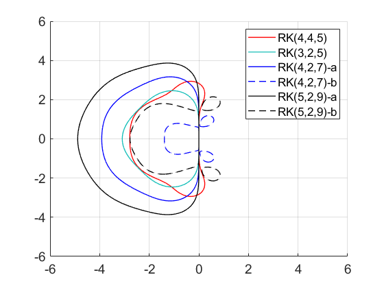
According to Propostion 2, when , an -stage method achieves the best energy accuracy if the set of coefficients forms a solution to the system of equations: for . For , the coefficients are listed in Table 1, and the stability regions of these second-order methods and a fourth-order method are shown in Figure 1. The RK(4,4,5) method is the classical fourth-order RK method, known as the RK4. Most methods have comparable or larger stability regions than the RK4, except RK(4,2,7)-b and RK(5,2,9)-b.
| method | ||||||||
|---|---|---|---|---|---|---|---|---|
| RK(3,2,5) | 3 | 2 | 5 | 1 | - | - | ||
| RK(4,2,7)-a | 4 | 2 | 7 | 1 | - | |||
| RK(4,2,7)-b | 4 | 2 | 7 | 1 | - | |||
| RK(5,2,9)-a | 5 | 2 | 9 | 1 | ||||
| RK(5,2,9)-b | 5 | 2 | 9 | 1 |
When , the leading coefficient , and the method is not strongly stable [6]. To obtain strongly stable methods, we consider , where the energy accuracy can reach an order of , given that there exists a solution to the system of equations for . For example, when we get
| (22) | |||||
| (23) | |||||
| (24) | |||||
| (25) | |||||
| (26) | |||||
| (27) | |||||
| (28) |
If , then , , , , and . Thus, by setting , we obtain a system of three equations with three unknowns , , and :
| (29) |
System (29) has one positive solution: , , and . Furthermore, in this case, we can verify that the leading coefficient , so the method is strongly stable, as Theorem 2.7 in [6] has proven that a negative leading coefficient implies strong stability. Similarly, we can calculate the coefficients and verify the strong stability for and . Additionally, we can find the strong stability criterion using Lemma 1 and it is summarized in the following theorem.
Theorem 1.
For an -stage, fourth-order RK method applied to system (1), if the coefficients form a solution to the system of equations for , and , then the order of energy accuracy is . Furthermore, the method is strongly stable if
| (30) |
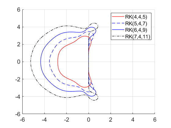
Table 2 lists the coefficients of four- to seven-stage methods of order four and the corresponding values in the strong stability criterion (30). Only coefficients with indices larger than are listed, as if . Additionally, the stability regions are illustrated in Figure 2. It demonstrates that as increases, the stability region expands.
| method | ||||||||
|---|---|---|---|---|---|---|---|---|
| RK(4,4,5) | 4 | 4 | 5 | - | - | - | ||
| RK(5,4,7) | 5 | 4 | 7 | - | - | |||
| RK(6,4,9) | 6 | 4 | 9 | - | ||||
| RK(7,4,11) | 7 | 4 | 11 |
Because the order of energy accuracy exceeds that of both the solution and the number of stages, we refer to it as the energy superconvergence phenomenon, and we term the corresponding RK method the energy-superconvergent RK (ESC-RK) method.
To construct an -stage RK method using the coefficients , we can use the following algorithm:
| (31) |
where
| (32) |
3 Examples
In this section, various ODE systems are simulated using the proposed methods, including second-order ODEs for harmonic oscillators, one-dimensional integro-differential equation for peridynamics, and the ODE systems derived from the semi-discretized one-dimensional Maxwell’s equations of electrodynamics.
The convergence of the solution is measured using standard , , and error norms, denoted by , , and , respectively. To test the energy accuracy, we calculate the convergence rate of the relative energy deviation:
| (33) |
where and represent the energy at the initial and the final times, respectively.
3.1 Second-order differential equation for harmonic oscillator
In the first example, we consider the second-order differential equation for a harmonic oscillator:
| (34) |
This equation can be written in matrix form as:
| (35) |
where and . The total energy of this system is given by:
| (36) |
where .
In our simulations, we set , , , and . The exact solution is . We use a uniform time step for all methods, where represents the number of grid points.
Table 3 presents the results obtained from several second-order RK methods, with coefficients provided in Table 1, along with the Störmer–Verlet (SV) method [9]. We adopt RK(4,2,7)-a and RK(5,2,9)-a due to their larger stability regions compared to their corresponding b-versions. These results illustrate the convergence rates of these methods, including their orders of energy accuracy. Notably, when , the relative energy deviation of RK(5,2,9) achieves machine precision (). Regarding the solution accuracy, the RK(3,2,5) has similar accuracy to the SV method, and as increases, the errors decreases. For this set of second-order RK methods, the relative energy deviations are positive, indicating that these methods are not strongly stable.
The results of fourth-order methods are presented in Table 4. Similar to the second-order methods, the errors decrease as increases. However, unlike the second-order methods, the relative energy deviations are all negative, indicating strong stability. We compare the performance of various fourth-order methods, as illustrated in Table 5. In this test, the 7-stage method exhibits better computational efficiency than the 4-stage method as it achieves a smaller error with a coarser mesh (). It’s worth noting that the 7-stage method has a larger step size limit (refer to Table 2), so better efficiency can be achieved if we use a larger .
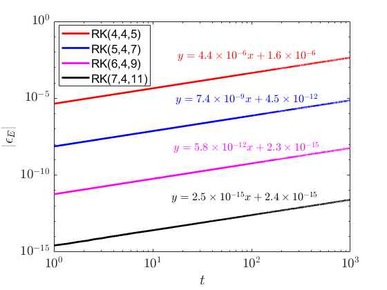
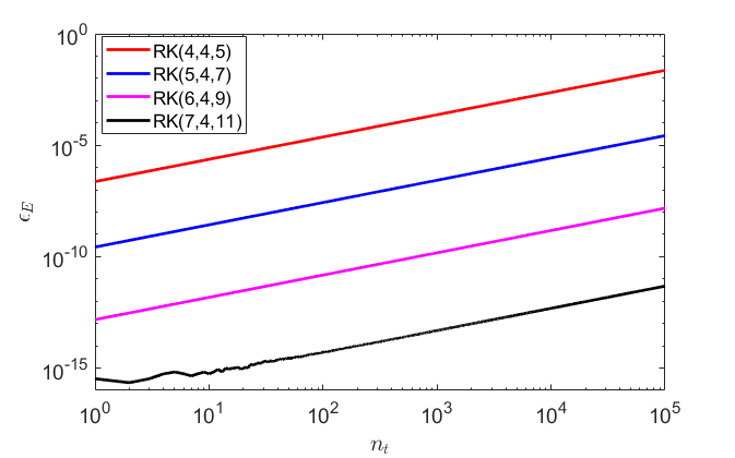
To assess energy dissipation, we conduct long time simulations () with . Figure 3 illustrates the time history plots of the magnitude of relative energy deviations for the fourth-order methods, along with the corresponding linear fitting lines. The slope of the fitting lines decrease by several orders of magnitude as increases by one, indicating a significant improvement in energy accuracy when superconvergent methods are used.
| Method | Order | Order | Order | Order | |||||
|---|---|---|---|---|---|---|---|---|---|
| SV | 100 | 6.62E-01 | 8.30E-02 | 1.77E+00 | -5.43E-02 | ||||
| 200 | 1.74E-01 | 1.93 | 1.57E-02 | 2.40 | 5.30E-01 | 1.74 | -3.30E-02 | 0.72 | |
| 400 | 4.28E-02 | 2.02 | 2.74E-03 | 2.52 | 1.34E-01 | 1.99 | -9.99E-03 | 1.72 | |
| 800 | 1.06E-02 | 2.01 | 4.82E-04 | 2.51 | 3.32E-02 | 2.01 | -2.49E-03 | 2.01 | |
| 1600 | 2.65E-03 | 2.00 | 8.50E-05 | 2.50 | 8.29E-03 | 2.00 | -6.18E-04 | 2.01 | |
| RK(3,2,5) | 100 | 7.54E-01 | 9.49E-02 | 2.02E+00 | 5.05E-01 | ||||
| 200 | 1.79E-01 | 2.08 | 1.62E-02 | 2.55 | 5.46E-01 | 1.89 | 1.29E-02 | 5.29 | |
| 400 | 4.31E-02 | 2.05 | 2.76E-03 | 2.55 | 1.35E-01 | 2.02 | 4.00E-04 | 5.01 | |
| 800 | 1.06E-02 | 2.02 | 4.83E-04 | 2.52 | 3.33E-02 | 2.02 | 1.25E-05 | 5.00 | |
| 1600 | 2.65E-03 | 2.00 | 8.50E-05 | 2.50 | 8.29E-03 | 2.00 | 3.91E-07 | 5.00 | |
| RK(4,2,7)-a | 100 | 3.49E-01 | 4.45E-02 | 9.70E-01 | 7.75E-03 | ||||
| 200 | 8.41E-02 | 2.05 | 7.63E-03 | 2.54 | 2.62E-01 | 1.89 | 6.03E-05 | 7.01 | |
| 400 | 2.07E-02 | 2.02 | 1.33E-03 | 2.52 | 6.47E-02 | 2.02 | 4.71E-07 | 7.00 | |
| 800 | 5.16E-03 | 2.01 | 2.34E-04 | 2.51 | 1.61E-02 | 2.01 | 3.68E-09 | 7.00 | |
| 1600 | 1.29E-03 | 2.00 | 4.12E-05 | 2.50 | 4.02E-03 | 2.00 | 2.87E-11 | 7.00 | |
| RK(5,2,9)-a | 100 | 2.05E-01 | 2.64E-02 | 6.17E-01 | 8.53E-05 | ||||
| 200 | 5.03E-02 | 2.03 | 4.56E-03 | 2.53 | 1.57E-01 | 1.98 | 1.67E-07 | 9.00 | |
| 400 | 1.24E-02 | 2.01 | 7.97E-04 | 2.51 | 3.88E-02 | 2.01 | 3.25E-10 | 9.00 | |
| 800 | 3.10E-03 | 2.01 | 1.40E-04 | 2.51 | 9.68E-03 | 2.00 | 6.31E-13 | 9.01 | |
| 1600 | 7.74E-04 | 2.00 | 2.48E-05 | 2.50 | 2.42E-03 | 2.00 | - |
| Method | Order | Order | Order | Order | |||||
|---|---|---|---|---|---|---|---|---|---|
| RK(4,4,5) | 100 | 8.24E-02 | 1.04E-02 | 2.40E-01 | -2.85E-01 | ||||
| 200 | 5.43E-03 | 3.92 | 4.90E-04 | 4.41 | 1.63E-02 | 3.88 | -1.11E-02 | 4.68 | |
| 400 | 3.39E-04 | 4.00 | 2.17E-05 | 4.50 | 1.03E-03 | 3.99 | -3.54E-04 | 4.97 | |
| 800 | 2.12E-05 | 4.00 | 9.61E-07 | 4.50 | 6.54E-05 | 3.97 | -1.11E-05 | 4.99 | |
| 1600 | 1.32E-06 | 4.00 | 4.24E-08 | 4.50 | 4.12E-06 | 3.99 | -3.47E-07 | 5.00 | |
| RK(5,4,7) | 100 | 1.78E-02 | 2.26E-03 | 5.34E-02 | -9.15E-03 | ||||
| 200 | 9.62E-04 | 4.21 | 8.71E-05 | 4.70 | 2.98E-03 | 4.16 | -7.48E-05 | 6.93 | |
| 400 | 5.75E-05 | 4.06 | 3.69E-06 | 4.56 | 1.79E-04 | 4.06 | -5.91E-07 | 6.99 | |
| 800 | 3.55E-06 | 4.02 | 1.61E-07 | 4.52 | 1.11E-05 | 4.01 | -4.63E-09 | 7.00 | |
| 1600 | 2.21E-07 | 4.01 | 7.09E-09 | 4.51 | 6.91E-07 | 4.00 | -3.62E-11 | 7.00 | |
| RK(6,4,9) | 100 | 6.01E-03 | 7.66E-04 | 1.84E-02 | -1.16E-04 | ||||
| 200 | 3.49E-04 | 4.11 | 3.16E-05 | 4.60 | 1.08E-03 | 4.09 | -2.35E-07 | 8.95 | |
| 400 | 2.14E-05 | 4.03 | 1.37E-06 | 4.53 | 6.66E-05 | 4.02 | -4.62E-10 | 8.99 | |
| 800 | 1.33E-06 | 4.01 | 6.02E-08 | 4.51 | 4.15E-06 | 4.01 | -9.03E-13 | 9.00 | |
| 1600 | 8.29E-08 | 4.00 | 2.66E-09 | 4.50 | 2.59E-07 | 4.00 | - | ||
| RK(7,4,11) | 100 | 2.92E-03 | 3.72E-04 | 8.94E-03 | -8.13E-07 | ||||
| 200 | 1.74E-04 | 4.07 | 1.58E-05 | 4.56 | 5.39E-04 | 4.05 | -4.09E-10 | 10.96 | |
| 400 | 1.07E-05 | 4.02 | 6.88E-07 | 4.52 | 3.34E-05 | 4.01 | -2.03E-13 | 10.97 | |
| 800 | 6.68E-07 | 4.01 | 3.03E-08 | 4.51 | 2.08E-06 | 4.00 | - | ||
| 1600 | 4.17E-08 | 4.00 | 1.34E-09 | 4.50 | 1.30E-07 | 4.00 | - |
| method | error norm | energy error | CPU time (seconds) | |
|---|---|---|---|---|
| RK(4,4,5) | 1600 | 4.24E-08 | -3.47E-07 | 0.073 |
| RK(5,4,7) | 800 | 1.61E-07 | -4.63E-09 | 0.045 |
| RK(6,4,9) | 800 | 6.02E-08 | -4.62E-10 | 0.054 |
| RK(7,4,11) | 800 | 3.03E-08 | 0.060 |
3.2 Linear peridynamic integro-differential equation
The theory of peridynamics [8] can be employed to model the nonlocal wave interaction of a homogeneous and infinitely long bar. The governing equation is a one-dimensional nonlocal integro-differential equation, which in the linear case, can be written as
| (37) |
where , , , and represent the displacement field, the density, the external force, and the micromodulus function, respectively. In this test, we utilize a normal distribution for the micromodulus function
| (38) |
where represents the horizon. To discretize equation (37), we partition the domain into cells and define at the cell centers: , , where . The integral in equation (37) can be approximated using the midpoint quadrature method:
| (39) |
Let , and assuming is constant, we can write the semi-discretized equation in matrix form:
| (40) |
where
| (41) |
and the entries of the matrix is defined by
| (42) |
System (40) can be written as a system of first-order equations:
| (43) | |||||
| (44) |
and in its matrix form, we have:
| (45) |
The total energy (Hamiltonian) of the system is:
| (46) |
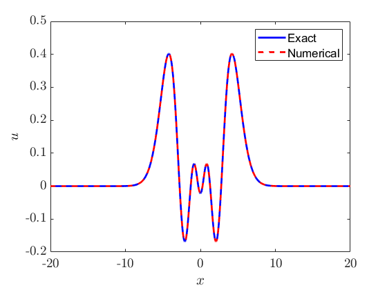
In our simulations, we set , , and . The computational domain is and . We let . The initial condition is and . Similar to previous studies [10, 11], a periodic boundary condition is implemented to approximate the original problem of an infinitely long bar. The simulation run until so that it stops before the solution reaches the boundaries. The exact solution is given by [12]:
| (47) |
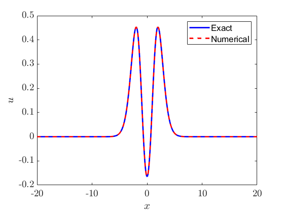
The solutions at two time snapshots using the seven-stage method RK(7,4,11) are shown in Figure 4. Results on convergence rates are presented in Table 6. All methods provide fourth-order accurate solutions, but the accuracy improves with larger due to better energy accuracy.
A comparison of computational cost is illustrated in Table 7, where the seven-stage method RK(7,4,11) demonstrates greater efficiency than the four-stage RK(4,4,5). The RK(7,4,11) method achieves a smaller error with half the mesh size and runs more than four times faster than RK(4,4,5). Additionally, the total energy of the RK(7,4,11) solution reaches machine precision at the final time when . The solution to peridynamic equations involves the evaluation of an integral every iteration, so doubling the mesh significantly increases the computational cost in terms of both memory and CPU run time.
| Method | Order | Order | Order | Order | |||||
|---|---|---|---|---|---|---|---|---|---|
| RK(4,4,5) | 100 | 2.62E-04 | - | 5.70E-05 | - | 2.05E-03 | - | -5.86E-03 | - |
| 200 | 1.58E-05 | 4.05 | 2.47E-06 | 4.53 | 1.26E-04 | 4.03 | -1.85E-04 | 4.99 | |
| 400 | 9.63E-07 | 4.04 | 1.05E-07 | 4.56 | 7.52E-06 | 4.06 | -5.84E-06 | 4.98 | |
| 800 | 5.93E-08 | 4.02 | 4.53E-09 | 4.53 | 4.62E-07 | 4.02 | -1.83E-07 | 5.00 | |
| 1600 | 3.67E-09 | 4.01 | 1.98E-10 | 4.52 | 2.87E-08 | 4.01 | -5.72E-09 | 5.00 | |
| RK(5,4,7) | 100 | 4.42E-05 | - | 9.47E-06 | - | 3.37E-04 | - | -1.08E-04 | - |
| 200 | 2.59E-06 | 4.09 | 3.94E-07 | 4.59 | 2.02E-05 | 4.06 | -8.32E-07 | 7.01 | |
| 400 | 1.57E-07 | 4.05 | 1.69E-08 | 4.54 | 1.22E-06 | 4.05 | -6.55E-09 | 6.99 | |
| 800 | 9.75E-09 | 4.01 | 7.41E-10 | 4.51 | 7.60E-08 | 4.00 | -5.12E-11 | 7.00 | |
| 1600 | 6.08E-10 | 4.00 | 3.27E-11 | 4.50 | 4.74E-09 | 4.00 | -4.00E-13 | 7.00 | |
| RK(6,4,9) | 100 | 1.53E-05 | - | 3.27E-06 | - | 1.20E-04 | - | -9.68E-07 | - |
| 200 | 9.51E-07 | 4.01 | 1.44E-07 | 4.51 | 7.38E-06 | 4.02 | -1.86E-09 | 9.02 | |
| 400 | 5.86E-08 | 4.02 | 6.30E-09 | 4.51 | 4.54E-07 | 4.02 | -3.66E-12 | 8.99 | |
| 800 | 3.65E-09 | 4.00 | 2.78E-10 | 4.50 | 2.84E-08 | 4.00 | -7.55E-15 | 8.92 | |
| 1600 | 2.28E-10 | 4.00 | 1.23E-11 | 4.50 | 1.77E-09 | 4.00 | - | ||
| RK(7,4,11) | 100 | 7.54E-06 | - | 1.61E-06 | - | 5.88E-05 | - | -5.06E-09 | - |
| 200 | 4.76E-07 | 3.99 | 7.20E-08 | 4.48 | 3.69E-06 | 3.99 | -2.43E-12 | 11.02 | |
| 400 | 2.94E-08 | 4.02 | 3.16E-09 | 4.51 | 2.28E-07 | 4.02 | -1.11E-15 | 11.10 | |
| 800 | 1.84E-09 | 4.00 | 1.40E-10 | 4.50 | 1.43E-08 | 4.00 | - | ||
| 1600 | 1.15E-10 | 4.00 | 6.18E-12 | 4.50 | 8.89E-10 | 4.01 | - |
| method | error norm | energy error | CPU time (seconds) | |
|---|---|---|---|---|
| RK(4,4,5) | 1600 | 1.98E-10 | -5.72E-09 | 17.40 |
| RK(5,4,7) | 800 | 7.41E-10 | -5.12E-11 | 2.77 |
| RK(6,4,9) | 800 | 2.78E-10 | -3.66E-12 | 3.30 |
| RK(7,4,11) | 800 | 1.40E-10 | 3.66 |
3.3 One-dimensional Maxwell’s equations
Consider the one-dimensional Maxwell’s equations
| (48) | |||||
| (49) |
By employing a staggered grid and centered difference algorithm, we define and , yielding the semi-discrete equations:
| (50) | |||||
| (51) |
These equations can be written in matrix form as:
| (52) |
where matrix represent the finite difference curl operator, and and are the solution vectors at time . For perfect electric conductor (PEC) boundaries, we have . is outside the boundary and is set to zero. For example, when , we have:
| (53) |
It can be verified that where stands for the spectral radius of a matrix. Thus, we have:
| (54) |
For the fourth-order RK methods in this work, the corresponding stability condition becomes , where is the speed of light and is given in Table 2.
The total energy of the system is given by
| (55) |
Note that if we define the magnetic field at time , and discretize the equations (50)-(51) using the leapfrog algorithm, we obtained the standard Yee Finite-Difference Time-Domain (FDTD) method [13, 14, 15]. Different from the energy defined in (55), the FDTD method preserves the following numerical energy:
| (56) |
In our simulations, the computational domain covers and with PEC boundaries. The initial condition is a Gaussian pulse defined as
| (57) |
with a carrier wavelength of . The simulation runs until , ensuring it stops before the solution reaches the boundaries. The exact solution is obtained using traveling wave solution: .
The simulation results are summarized in Table 8. All four RK methods exhibit similar accuracy, with convergence rates of the solutions being second-order due to the spatial discretization being second-order. To assess computational efficiency, we compare against the FDTD method. For FDTD, we choose a Courant number of 1, so . As shown in Table 9, the fourth-order RK methods achieve better accuracy and run faster than the fine mesh FDTD result. The RK methods do not significantly increase the computational cost, partly because they use larger (equivalently, smaller ). In this simulation, both the six- and seven-stage methods achieve energy accuracy of machine precision at the final time when the grid size is .
To compare the energy dissipation over a long time, we run the simulations for 100,000 iterations with the same Courant number of 0.5 () for all methods. The computational mesh size is fixed at , resulting in a resolution of 20 cells per wavelength (). The results are shown in Figure 5. At the end of the simulation (), the energy dissipation decreases by approximately 3 orders of magnitude as increases by one. Specifically, the energy dissipation of the RK(4,4,5) method is about 0.02, compared to for the RK(7,4,11) method. This demonstrates that the energy accuracy can be significantly enhanced by employing superconvergent methods.
| Method | Order | Order | Order | Order | |||||
|---|---|---|---|---|---|---|---|---|---|
| RK(4,4,5) | 2000 | 3.8414E-03 | 2.3641E-04 | 5.2370E-02 | -8.07E-04 | ||||
| 4000 | 9.4638E-04 | 2.02 | 4.1187E-05 | 2.52 | 1.2910E-02 | 2.02 | -2.55E-05 | 4.98 | |
| 8000 | 2.3568E-04 | 2.01 | 7.2527E-06 | 2.51 | 3.2140E-03 | 2.01 | -7.99E-07 | 5.00 | |
| 16000 | 5.8863E-05 | 2.00 | 1.2809E-06 | 2.50 | 8.0279E-04 | 2.00 | -2.50E-08 | 5.00 | |
| 32000 | 1.4712E-05 | 2.00 | 2.2638E-07 | 2.50 | 2.0064E-04 | 2.00 | -7.81E-10 | 5.00 | |
| RK(5,4,7) | 2000 | 3.7922E-03 | 2.3330E-04 | 5.1708E-02 | -7.72E-06 | ||||
| 4000 | 9.4262E-04 | 2.01 | 4.1024E-05 | 2.51 | 1.2851E-02 | 2.01 | -6.11E-08 | 6.98 | |
| 8000 | 2.3551E-04 | 2.00 | 7.2475E-06 | 2.50 | 3.2120E-03 | 2.00 | -4.79E-10 | 6.99 | |
| 16000 | 5.8839E-05 | 2.00 | 1.2803E-06 | 2.50 | 8.0245E-04 | 2.00 | -3.74E-12 | 7.00 | |
| 32000 | 1.4711E-05 | 2.00 | 2.2636E-07 | 2.50 | 2.0063E-04 | 2.00 | -3.16E-14 | 6.89 | |
| RK(6,4,9) | 2000 | 3.7854E-03 | 2.3286E-04 | 5.1611E-02 | -3.55E-08 | ||||
| 4000 | 9.4187E-04 | 2.01 | 4.0992E-05 | 2.51 | 1.2837E-02 | 2.01 | -7.03E-11 | 8.98 | |
| 8000 | 2.3531E-04 | 2.00 | 7.2414E-06 | 2.50 | 3.2092E-03 | 2.00 | -1.39E-13 | 8.99 | |
| 16000 | 5.8843E-05 | 2.00 | 1.2804E-06 | 2.50 | 8.0249E-04 | 2.00 | - | ||
| 32000 | 1.4711E-05 | 2.00 | 2.2635E-07 | 2.50 | 2.0062E-04 | 2.00 | - | ||
| RK(7,4,11) | 2000 | 3.7724E-03 | 2.3225E-04 | 5.1375E-02 | -6.12E-11 | ||||
| 4000 | 9.4246E-04 | 2.00 | 4.1015E-05 | 2.50 | 1.2854E-02 | 2.00 | -3.01E-14 | 10.99 | |
| 8000 | 2.3534E-04 | 2.00 | 7.2423E-06 | 2.50 | 3.2098E-03 | 2.00 | - | ||
| 16000 | 5.8833E-05 | 2.00 | 1.2802E-06 | 2.50 | 8.0237E-04 | 2.00 | - | ||
| 32000 | 1.4711E-05 | 2.00 | 2.2636E-07 | 2.50 | 2.0063E-04 | 2.00 | - |
| method | CPU time (seconds) | |||||||
|---|---|---|---|---|---|---|---|---|
| FDTD | 32000 | 9593 | 1.0 | 1.76E-04 | 2.74E-06 | 2.45E-03 | 2.09 | |
| RK(4,4,5) | 16000 | 3392 | 5.88E-05 | 1.28E-06 | 8.02E-04 | -2.50E-08 | 1.31 | |
| RK(5,4,7) | 16000 | 2769 | 5.88E-05 | 1.28E-06 | 8.02E-04 | -3.74E-12 | 1.32 | |
| RK(6,4,9) | 16000 | 2477 | 5.88E-05 | 1.28E-06 | 8.02E-04 | 1.39 | ||
| RK(7,4,11) | 16000 | 2398 | 2.0 | 5.88E-05 | 1.28E-06 | 8.02E-04 | 1.54 |
4 Conclusion
Through the study of energy convergence rates of explicit Runge-Kutta (RK) methods for antisymmetric linear autonomous systems, we have developed a class of energy-superconvergent RK methods in which the orders of energy accuracy exceed the number of stages. For an -stage RK method of an even order , the energy accuracy can achieve up to an order of . Generally, higher order energy accuracy leads to a larger stability region and thus a larger step size. Additionally, we have derived the strong stability criteria for several fourth-order methods when . We present numerical solutions of ODEs for harmonic oscillators and nonlocal integro-differential equations for peridynamics, demonstrating that the energy error can reach machine precision for methods with higher-order energy accuracy. When comparing methods with the same solution orders but different energy accuracy, the error due to time discretization decreases as the order of energy accuracy increases. A method with higher-order energy accuracy exhibits comparable computational efficiency to lower-order ones. Furthermore, the proposed RK methods are used as the time discretization method for the semi-discretized one-dimensional Maxwell’s equations on a spatially staggered grid, similar to the Yee FDTD method. While the RK-based methods maintain second-order accuracy due to spatial discretization, they offer superior accuracy and permit larger time steps than the FDTD method, leading to better efficiency.
References
- [1] Doron Levy and Eitan Tadmor. From semidiscrete to fully discrete: Stability of runge–kutta schemes by the energy method. SIAM review, 40(1):40–73, 1998.
- [2] Sigal Gottlieb and Chi-Wang Shu. Total variation diminishing runge-kutta schemes. Mathematics of computation, 67(221):73–85, 1998.
- [3] Sigal Gottlieb, Chi-Wang Shu, and Eitan Tadmor. Strong stability-preserving high-order time discretization methods. SIAM review, 43(1):89–112, 2001.
- [4] Eitan Tadmor. From semidiscrete to fully discrete: stability of runge-kutta schemes by the energy method. ii. Collected lectures on the preservation of stability under discretization, 109:25–49, 2002.
- [5] Zheng Sun and Chi-Wang Shu. Stability of the fourth order runge–kutta method for time-dependent partial differential equations. Annals of Mathematical Sciences and Applications, 2(2):255–284, 2017.
- [6] Zheng Sun and Chi-Wang Shu. Strong stability of explicit runge–kutta time discretizations. SIAM Journal on Numerical Analysis, 57(3):1158–1182, 2019.
- [7] Bernardo Cockburn and Chi-Wang Shu. Runge–kutta discontinuous galerkin methods for convection-dominated problems. Journal of scientific computing, 16:173–261, 2001.
- [8] Stewart A Silling. Reformulation of elasticity theory for discontinuities and long-range forces. Journal of the Mechanics and Physics of Solids, 48(1):175–209, 2000.
- [9] Ernst Hairer, Christian Lubich, and Gerhard Wanner. Geometric numerical integration illustrated by the störmer–verlet method. Acta numerica, 12:399–450, 2003.
- [10] Giuseppe Maria Coclite, Alessandro Fanizzi, Luciano Lopez, Francesco Maddalena, and Sabrina Francesca Pellegrino. Numerical methods for the nonlocal wave equation of the peridynamics. Applied Numerical Mathematics, 155:119–139, 2020.
- [11] Jinjie Liu, Samuel Appiah-Adjei, and Moysey Brio. Iterated crank–nicolson method for peridynamic models. Dynamics, 4(1):192–207, 2024.
- [12] Olaf Weckner and Rohan Abeyaratne. The effect of long-range forces on the dynamics of a bar. Journal of the Mechanics and Physics of Solids, 53(3):705–728, 2005.
- [13] Kane Yee. Numerical solution of initial boundary value problems involving maxwell’s equations in isotropic media. IEEE Transactions on antennas and propagation, 14(3):302–307, 1966.
- [14] A. Taflove and M. E. Brodwin. Numerical solution of steady-state electromagnetic scattering problems using the time-dependent Maxwell’s equations. IEEE Trans. Microwave Theory Tech., 23:623–630, 1975.
- [15] A. Taflove and S. Hagness. Computational Electrodynamics: The Finite-Difference Time-Domain Method. Artech House, Norwood, MA, 3rd edition, 2005.