Robust Reward Placement under Uncertainty

Abstract

We consider a problem of placing generators of rewards to be collected by randomly moving agents in a network. In many settings, the precise mobility pattern may be one of several possible, based on parameters outside our control, such as weather conditions. The placement should be robust to this uncertainty, to gain a competent total reward across possible networks. To study such scenarios, we introduce the Robust Reward Placement problem (RRP). Agents move randomly by a Markovian Mobility Model with a predetermined set of locations whose connectivity is chosen adversarially from a known set $\Pi$ of candidates. We aim to select a set of reward states within a budget that maximizes the minimum ratio, among all candidates in $\Pi$, of the collected total reward over the optimal collectable reward under the same candidate. We prove that RRP is NP-hard and inapproximable, and develop $\Psi$-Saturate, a pseudo-polynomial time algorithm that achieves an $\epsilon$-additive approximation by exceeding the budget constraint by a factor that scales as $\mathcal{O}(\ln|\Pi|/\epsilon)$. In addition, we present several heuristics, most prominently one inspired by a dynamic programming algorithm for the $\max$–$\min$ 0–1 Knapsack problem. We corroborate our theoretical analysis with an experimental evaluation on synthetic and real data.

1 Introduction

In many graph optimization problems, a stakeholder has to select locations in a network, such as a road, transportation, infrastructure, communication, or web network, where to place reward-generating facilities such as stores, ads, sensors, or utilities to best service a population of moving agents such as customers, autonomous vehicles, or bots [?; ?; ?; ?; ?]. Such problems are intricate due to the uncertainty surrounding agent mobility [?; ?; ?; ?].

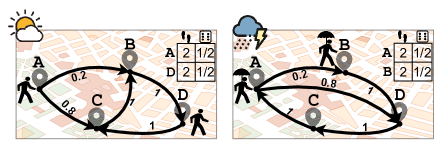
Figure 1: Moving agent under two settings; sunny and rainy; tables show numbers of steps and initial probabilities.

For instance, consider outdoor ad placement. We represent the road map as a probabilistic network in which agents move. If every agent follows the same movement pattern regardless of environmental conditions, then the problem of placing ads to maximize the expected number of ad views admits a greedy algorithm with an approximation ratio [?]. Still, the problem becomes more involved under malleable environmental conditions that alter movement patterns. As a toy example, Figure 1 shows a probabilistic network. An agent randomly starts from an initial location and takes two steps by the probabilities shown on edges representing street segments, under two environmental settings, sunny and rainy. Assume a stakeholder has a budget to place an ad-billboard at a single location. Under the sunny setting, the best choice of placement is $B$, as the agent certainly passes by that point regardless of its starting position; under the rainy setting, the agent necessarily passes by $D$ within two steps, hence that is most preferable. However, under the rainy setting $B$ yields expected reward $0.6$, and so does $D$ under the sunny one. Due to such uncertainty, a risk-averse stakeholder would prefer the location that yields, in the worst case, the highest ratio of the collected to best feasible reward, i.e., in this case, $C$, which yields expected reward $0.9$ under both settings.

In this paper, we introduce the problem of robust reward placement (RRP) in a network, under uncertainty about the environment whereby an agent is moving according to any of several probabilistic mobility settings. We express each such setting by a Markov Mobility Model (MMM) $\pi\leavevmode\nobreak\ \in\leavevmode\nobreak\ \Pi$. The cumulative reward a stakeholder receives grows whenever the agent passes by one of the reward states $\mathcal{S}_{\mathcal{R}}$. RRP seeks to select a set of such states $\mathcal{S}_{\mathcal{R}}^{*}$ within a budget, that maximizes the worst-case ratio, across all settings $\Pi$, of the collected reward ${F}(\mathcal{S}_{\mathcal{R}}|\pi)$ over the highest reward that can be collected under the same setting ${F}(\mathcal{S}^{*}_{\pi}|\pi)$, i.e., $\mathcal{S}_{\mathcal{R}}^{*}\leavevmode\nobreak\ =\leavevmode\nobreak\ \arg\max_{\mathcal{S}_{\mathcal{R}}}\min_{\pi\in\Pi}\frac{{F}(\mathcal{S}_{\mathcal{R}}|\pi)}{{F}(\mathcal{S}^{*}_{\pi}|\pi)}$. This max-min ratio objective is used in risk-averse portfolio optimization and advertising [?; ?].

Our Contribution.

Our contributions stand as follows:

1. We introduce the problem of Robust Reward Placement (RRP) over a set of Markov Mobility Models, that has real-world applications across various domains.

2. We study the properties of RRP and show that it is $\mathbf{NP}$-hard (Theorem 1). Due to the additivity and monotonicity properties of the reward function (Lemma 3), it admits an optimal solution in pseudo-polynomial time under a single setting, i.e. $|\Pi|=1$ (Lemma 4), yet it is inapproximable when $|\Pi|>1$ unless we exceed the budget constraint by a factor $\mathcal{O}(\ln|\Pi|)$ (Theorem 2).

3. We adopt techniques from robust influence maximization to develop $\Psi$-Saturate, a pseudo-polynomial time algorithm that finds a solution within $\epsilon$ distance of the optimal, i.e. $\text{OPT}-\epsilon$, while exceeding the budget constraint by an $\mathcal{O}(\ln\nicefrac{{|\Pi|}}{{\epsilon}})$ factor (Lemma LABEL:lem:bicriteria_apx).

4. We present several heuristics as alternative solutions, most prominently one based on a dynamic programming algorithm for the $\max$–$\min$ 0–1 Knapsack problem, to which RRP can be reduced (Lemma 5).

We corroborate our analysis with an experimental evaluation on synthetic and real data. Due to space constraints, we relegate some proofs to the Appendix LABEL:sec:app.

2 Related Work

The Robust Reward Placement problem relates to robust maximization of spread in a network, with some distinctive characteristics. Some works [?; ?; ?; ?; ?] study problems of selecting a seed set of nodes that robustly maximize the expected spread of a diffusion process over a network. However, in those models [?] the diffusion process is generative, whereby an item propagates in the network by producing unlimited replicas of itself. On the other hand, we study a non-generative spread function, whereby the goal is to reach as many as possible out of a population of network-resident agents. Our spread function is similar to the one studied in the problem of Geodemographic Influence Maximization [?], yet thereby the goal is to select a set of network locations that achieves high spread over a mobile population under a single environmental setting. We study the more challenging problem of achieving competitive spread in the worst case under uncertainty regarding the environment.

Several robust discrete optimization problems [?] address uncertainty in decision-making by optimizing a $\max$–$\min$ or $\min$–$\max$ function under constraints. The robust Minimum Steiner Tree problem [?] seeks to minimize the worst-case cost of a tree that spans a graph; the $\min$–$\max$ and $\min$–$\max$ regret versions of the Knapsack problem [?] have a modular function as a budget constraint; other works examine the robust version of submodular functions [?; ?] that describe several diffusion processes [?; ?]. To our knowledge, no prior work considers the objective of maximizing the worst-case ratio of an additive function over its optimal value subject to a knapsack budget constraint.

3 Preliminaries

Markov Mobility Model (MMM).

We denote a discrete-time MMM as $\pi=(\mathcal{S},{\mathcal{I}},\mathcal{T},{\mathcal{M}})$, where $\mathcal{S}$ is a set of $n$ states, ${\mathcal{I}}$ is a vector of $n$ elements in $[0,1]$ expressing an initial probability distribution over states in $\mathcal{S}$, $\mathcal{T}$ is an $n\times n$ right-stochastic matrix, where $\mathcal{T}[s,s^{\prime}]$ is the probability of transition from state $s\in\mathcal{S}$ to another state $s^{\prime}\in\mathcal{S}$, and ${\mathcal{M}}$ is an $n\times K$ matrix with elements in $[0,1]$, where $K$ is the maximum number of steps and ${\mathcal{M}}[s,k]$ expresses the cumulative probability that an agent starting from state $s\in\mathcal{S}$ takes $k^{\prime}\in[k,K]$ steps. Remarkably, an MMM describes multiple agents and movements, whose starting positions are expressed via initial distribution ${\mathcal{I}}$ and their step-sizes via ${\mathcal{M}}$.

Rewards.

Given an MMM, we select a set of states to be reward states. We use a reward vector $\mathcal{R}\in\{0,1\}^{n}$ to indicate whether state $s\in\mathcal{S}$ is a reward state and denote the set of reward states as $\mathcal{S}_{\mathcal{R}}=\{s\in\mathcal{S}|\mathcal{R}[s]=1\}$. In each timestamp $t$, an agent at state $s$ moves to state $s^{\prime}$ and retrieves reward $\mathcal{R}[s^{\prime}]$. For a set of reward states $\mathcal{S}_{\mathcal{R}}$, and a given MMM $\pi$, the cumulative reward ${F}(\mathcal{S}_{\mathcal{R}}|\pi)$ of an agent equals:

$${F}(\mathcal{S}_{\mathcal{R}}|\pi) =\sum_{k\in[K]}{F}_{\pi}(\mathcal{S}_{\mathcal{R}}|k)$$ (1)

$${F}_{\pi}(\mathcal{S}_{\mathcal{R}}|k) =\mathcal{R}^{\top}\left(\mathcal{T}^{k}({\mathcal{I}}\circ{\mathcal{M}}_{k})\right),$$ (2)

where ${F}_{\pi}(\mathcal{S}_{\mathcal{R}}|k)$ is the expected reward at the $k^{\text{th}}$ step, ${\mathcal{M}}_{k}$ is the $k^{\text{th}}$ column of ${\mathcal{M}}$, and $\circ$ denotes the Hadamard product.

Connection to Pagerank.

The Pagerank algorithm [?], widely used in recommendation systems, computes the stationary probability distribution of a random walker in a network. The Pagerank scores are efficiently computed via power-iteration method [?]. Let $\mathbf{PR}$ be an $N\times 1$ column-vector of the Pagerank probability scores, initialized as $\mathbf{PR}(0)$, $\mathbf{T}$ is an $N\times N$ matrix featuring the transition probabilities of walker, and $\mathbf{1}$ be the all-ones vector. For a damping factor $a$, the power method computes the scores in iterations as:

$$\mathbf{PR}(t)=a\cdot\mathbf{T}\cdot\mathbf{PR}(t-1)+\frac{1-a}{N}\mathbf{1}.$$ (3)

We repeat this process until convergence, i.e., until $|\mathbf{PR}(t)-\mathbf{PR}(t-1)|\leq\epsilon$ for a small $\epsilon\geq 0$. We denote the PageRank score at the $i^{th}$ node as $\mathbf{PR}[i]$. For a sufficiently large number of steps $K$ for each state with ${\mathcal{M}}_{k}\!=\!\mathbf{1}\,\forall k\!\in\![K]$, Equation (2) becomes ${F}_{\pi}(k)=\mathcal{R}^{\top}\left(\mathcal{T}^{k}{\mathcal{I}}\right)$. Likewise, for damping factor $a=1$, Equation (3) becomes $\mathbf{PR}(t)=\mathbf{T}^{t}\mathbf{PR}(0)$, thus the two equations are rendered analogous with $\mathbf{T}=\mathcal{T}$ and $\mathbf{PR}(0)={\mathcal{I}}$. Then, considering that the iteration converges from step $\hat{k}$ onward, the expected reward from reward state $s_{i}$ per step $k\geq\hat{k}$, ${F}_{\pi}(\{s_{i}\}|k)$, is the PageRank score of the $i^{\mathrm{th}}$ node, that is $\mathbf{PR}[i]$. To see this, let $\mathcal{R}_{i}=\mathbf{1}_{i}$ be the reward vector when $s_{i}\in\mathcal{S}$ is the only reward state; then it holds that $\mathbf{PR}[i]=\mathbf{1}_{i}^{\top}\left(\mathbf{T}^{k}\mathbf{PR}(0)\right)=\mathcal{R}_{i}^{\top}\left(\mathcal{T}^{k}{\mathcal{I}}\right)={F}_{\pi}(\{s_{i}\}|k)$.

4 Problem Formulation

In this section we model the uncertain environment where individuals navigate and introduce the Robust Reward Placement (RRP) problem over a set of Markov Mobility Models (MMMs), extracted from real movement data, that express the behavior of individuals under different settings.

Setting.

Many applications generate data on the point-to-point movements of agents over a network, along with a distribution and their total number of steps. Using aggregate statistics on this information, we formulate, without loss of generality, the movement of a population by a single agent moving probabilistically over the states of an MMM $\pi=(\mathcal{S},{\mathcal{I}},\mathcal{T},{\mathcal{M}})$. Due to environment uncertainty, the agent may follow any of $|\Pi|$ different settings $\Pi=\{\pi_{1},\pi_{2},\ldots,\pi_{|\Pi|}\}$.

Robust Reward Placement Problem.

Several resource allocation problems can be formulated as optimization problems over an MMM $\pi$, where reward states $\mathcal{S}_{\mathcal{R}}$ correspond to the placement of resources. Given a budget $L$ and a cost function $c:\mathcal{S}\rightarrow\mathbb{N}^{+}$, the Reward Placement (RP) problem seeks a set of reward states $\mathcal{S}_{\mathcal{R}}^{*}\subseteq\mathcal{S}$ that maximizes the cumulative reward ${F}(\mathcal{S}_{\mathcal{R}}^{*}|\pi)$ obtained by an agent, that is:

$$\mathcal{S}_{\mathcal{R}}^{*}=\arg\max_{\mathcal{S}_{\mathcal{R}}}{F}(\mathcal{S}_{\mathcal{R}}|\pi)\text{\quad s.t. }\sum_{s\in\mathcal{S}_{\mathcal{R}}}c[s]\leq L.$$

However, in reality the agent’s movements follow an unknown distribution sampled from a set of settings ${\Pi}\leavevmode\nobreak\ =\leavevmode\nobreak\ \{\pi_{1},\pi_{2},\ldots,\pi_{|\Pi|}\}$ represented as different MMMs. Under this uncertainty, the Robust Reward Placement (RRP) problem seeks a set of reward states $\mathcal{S}_{\mathcal{R}}$, within a budget, that maximizes the worst-case ratio of agent’s cumulative reward over the optimal one, when the model $\pi\in\Pi$ is unknown. Formally, we seek a reward placement $\mathcal{S}_{\mathcal{R}}^{*}\subseteq\mathcal{S}$ such that:

$$\mathcal{S}_{\mathcal{R}}^{*}=\arg\max_{\mathcal{S}_{\mathcal{R}}}\min_{\pi\in\Pi}\frac{{F}(\mathcal{S}_{\mathcal{R}}|\pi)}{{F}(\mathcal{S}^{*}_{\pi}|\pi)}\text{\quad s.t. }\sum_{s\in\mathcal{S}_{\mathcal{R}}}c[s]\leq L,$$ (4)

where $\mathcal{S}^{*}_{\pi}=\arg\max\limits_{\mathcal{S}_{\mathcal{R}}}{{F}(\mathcal{S}_{\mathcal{R}}|\pi)}$ is the optimal reward placement for a given model $\pi\in\Pi$ within budget $L$. This formulation is equivalent to minimizing the maximum regret ratio of ${F}(\mathcal{S}_{\mathcal{R}}|\pi)$, i.e., $1-\frac{{F}(\mathcal{S}_{\mathcal{R}}|\pi)}{{F}(\mathcal{S}^{*}_{\pi}|\pi)}$. The motivation arises from the fact that stakeholders are prone to compare what they achieve with what they could optimally achieve. The solution may also be seen as the optimal placement when the model $\pi\in\Pi$ in which agents are moving is chosen by an omniscient adversary, i.e. an adversary who chooses the setting $\pi$ after observing the set of reward states $\mathcal{S}_{\mathcal{R}}$.

5 Hardness and Inapproximability Results

In this section we examine the optimization problem of RRP and we show that is $\mathbf{NP}$-hard in general. First, in Theorem 1 we prove that even for a single model $(|\Pi|=1)$ the optimal solution cannot be found in polynomial time, due to a reduction from the 0–1 Knapsack problem [?].

Theorem 1.

The RRP problem is $\mathbf{NP}$-hard even for a single model, that is $|\Pi|=1$.

Proof.

In the 0–1 Knapsack problem [?] we are given a set of items $U$, each item $u\in U$ having a cost $c(u)$ and, wlog, an integer value $F(u)$ and seek a subset $V\subseteq U$ that has total cost $\sum_{v\in V}c(v)$ no more than a given budget $L$ and maximum total value $\sum_{v\in V}F(v)$. In order to reduce 0–1 Knapsack to RRP, we set a distinct state $s\leavevmode\nobreak\ \in\leavevmode\nobreak\ \mathcal{S}$ for each item $u\in U$ with the same cost, i.e., $\mathcal{S}=U$, assign to each state a self-loop with transition probability $1$, let each state be a reward state, and set a uniform initial distribution of agents over states equal to $\nicefrac{{1}}{{\left|\mathcal{S}\right|}}$ and steps probability equal to ${\mathcal{M}}[s,k]=1,\,\forall k\in[1,\ldots,F(u)]$. For a single setting, an optimal solution to the RRP problem of Equation (4) is also optimal for the $\mathbf{NP}$-hard 0–1 Knapsack problem.∎

Theorem 2 proves that RRP is inapproximable in polynomial time within constant factor, by a reduction from the Hitting Set problem, unless we exceed the budget constraint.

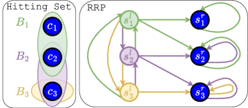
Figure 2: Hitting Set (left) and RRP reduction (right).

Theorem 2.

Given a budget $L$ and set of models $\Pi$, it is $\mathbf{NP}$-hard to approximate the optimal solution to RRP within a factor of $\Omega(\nicefrac{{1}}{{n^{1-\epsilon}}})$, for any constant $\epsilon>0$, unless the cost of the solution is at least $\beta L$, with $\beta\geq\ln|\Pi|$.

Proof.

We reduce the Hitting Set problem [?] to RRP and show that an approximation algorithm for RRP implies one for Hitting Set. In the Hitting Set problem, given a collection of $X$ items, $C=\{c_{1},c_{2},\ldots,c_{X}\}$ and a set of $M$ subsets thereof, $B_{i}\subseteq C$, $i\in\{1,\ldots,M\}$, we seek a hitting set $C^{\prime}\subseteq C$ such that $B_{i}\cap C^{\prime}\neq\emptyset\,\,\forall i\in\{1,\ldots,M\}$.

Given an instance of Hitting Set, we reduce it to RRP as follows. For each subset $B_{i}$ we set a state $s^{l}_{i}\in\mathcal{S}^{l}$ and for each item $c_{i}$ we set a state $s^{r}_{i}\in\mathcal{S}^{r}$. Aslo, for each subset $B_{i}$ we set an MMM $\pi_{i}$ $(|\Pi|=M)$ over the same set of states $\mathcal{S}=\mathcal{S}^{l}\cup\mathcal{S}^{r}$ with $\mathcal{S}^{l}\cap\mathcal{S}^{r}=\emptyset$. We set the initial probabilities ${\mathcal{I}}$ as uniform for all states in $\mathcal{S}^{l}$, equal to $\nicefrac{{1}}{{|\mathcal{S}^{l}|}}$ for all models. Each model $\pi_{i}\in\Pi$ features transition probabilities $1$ from each state $s^{l}_{j}$ to state $s^{l}_{i}$, with $i\neq j$, and uniform transition probabilities from $s^{l}_{i}$ to each state $s^{r}_{j}$ if and only if $c_{j}\in B_{i}$. States in $\mathcal{S}^{r}$ are absorbing, i.e., each state has a self-loop with probability $1$. Figure 2 shows a small example of a Hitting Set instance and its RRP equivalent. We set the cost for absorbing states in $\mathcal{S}^{r}$ to $1$ and let each node in $\mathcal{S}^{l}$ have a cost exceeding $L$. By this construction, if the reward placement $\mathcal{S}_{\mathcal{R}}$ does not form a hitting set, then there exists at least one subset $B_{i}$, such that $B_{i}\cap\mathcal{S}_{\mathcal{R}}=\emptyset$, hence $\min_{\pi}\frac{{F}(\mathcal{S}_{\mathcal{R}}|\pi)}{{F}(\mathcal{S}^{*}_{\pi}|\pi)}=0$. In reverse, if $\mathcal{S}_{\mathcal{R}}$ forms a hitting set, it holds that $\min_{\pi}\frac{{F}(\mathcal{S}_{\mathcal{R}}|\pi)}{{F}(\mathcal{S}^{*}_{\pi}|\pi)}\geq\frac{1}{|\mathcal{S}^{r}|}>0$. Thus, a hitting set exists if and only if $\min_{\pi}\frac{{F}(\mathcal{S}_{\mathcal{R}}|\pi)}{{F}(\mathcal{S}^{*}_{\pi}|\pi)}>0$. In effect, if we obtained an approximation algorithm for RRP by increasing the budget to $\beta L$, for $\beta>1$, then we would also approximate, with a budget increased by a factor of $\beta$, the Hitting Set problem, which is $\mathbf{NP}$-hard for $\beta<(1-\delta)\ln|\Pi|$ and $\delta>0$ [?]. ∎

6 Connections to Knapsack Problems

In this section, we establish connections between RRP and Knapsack problems, which are useful in our solutions.

Monotonicity and Additivity.

Lemma 3 establishes that the cumulative reward function ${F}(\mathcal{S}_{\mathcal{R}}|\pi)$ is monotone and additive with respect to $\mathcal{S}_{\mathcal{R}}$. These properties are vital in evaluating ${F}(\mathcal{S}_{\mathcal{R}}|\pi)$ while exploiting pre-computations.

Lemma 3.

The cumulative reward ${F}(\mathcal{S}_{\mathcal{R}}|\pi)$ in Equation (1) is a monotone and additive function of reward states $\mathcal{S}_{\mathcal{R}}$.

Proof.

By Equation (1) we obtain the monotonicity property of the cumulative reward function ${F}(\cdot|\pi)$. Given a model $\pi\in\Pi$ and two sets of reward states $\mathcal{A}\subseteq\mathcal{B}\subseteq\mathcal{S}$ every term of ${F}(\mathcal{A}|\pi)$ is no less than its corresponding term of ${F}(\mathcal{B}|\pi)$ due to Equation (2). For the additivity property it suffices to show that any two sets of reward states $\mathcal{A},\mathcal{B}\subseteq\mathcal{S}$ satisfy:

$${F}(\mathcal{A}|\pi)\leavevmode\nobreak\ +\leavevmode\nobreak\ {F}(\mathcal{B}|\pi)\leavevmode\nobreak\ =\leavevmode\nobreak\ {F}(\mathcal{A}\leavevmode\nobreak\ \cup\leavevmode\nobreak\ \mathcal{B}|\pi)\leavevmode\nobreak\ +\leavevmode\nobreak\ {F}(\mathcal{A}\cap\ \mathcal{B}|\pi).$$

Assume w.l.o.g. that the equality holds at time $t$, i.e. $r^{t}_{\mathcal{A}}+r^{t}_{\mathcal{B}}=r^{t}_{\mathcal{A}\cap\mathcal{B}}+r^{t}_{\mathcal{A}\cup\mathcal{B}}$, $r^{t}_{\mathcal{X}}$ being the cumulative reward at time $t$ for reward states $\mathcal{X}$. It suffices to prove that the additivity property holds for $t+1$. At timestamp $t+1$, the agent at state $s\in\mathcal{S}$ moves to $s^{\prime}\in\mathcal{S}$. We distinguish cases as follows:

1. If $s^{\prime}\notin\mathcal{A}\cup\mathcal{B}$ then $s^{\prime}\notin\mathcal{A}\cap\mathcal{B}$, $s^{\prime}\notin\mathcal{A}$ and $s^{\prime}\notin\mathcal{B}$, thus additivity holds.

2. If $s^{\prime}\in\mathcal{A}\cup\mathcal{B}$ and $s^{\prime}\notin\mathcal{A}\cap\mathcal{B}$ then either $s^{\prime}\in\mathcal{A}$ or $s^{\prime}\in\mathcal{B}$. Assume wlog that $s^{\prime}\in\mathcal{A}$, then it holds that: $r^{t+1}_{\mathcal{A}}=r^{t}_{\mathcal{A}}+\mathcal{T}[s,s^{\prime}]$, $r^{t+1}_{\mathcal{A}\cup\mathcal{B}}=r^{t}_{\mathcal{A}\cup\mathcal{B}}+\mathcal{T}[s,s^{\prime}]$, $r^{t+1}_{\mathcal{B}}=r^{t}_{\mathcal{B}}$ and $r^{t+1}_{\mathcal{A}\cap\mathcal{B}}=r^{t}_{\mathcal{A}\cap\mathcal{B}}$.

3. If $s^{\prime}\in\mathcal{A}\cap\mathcal{B}$ then $s^{\prime}\in\mathcal{A}$ and $s^{\prime}\in\mathcal{B}$. Then, it holds that: $r^{t+1}_{\mathcal{A}}=r^{t}_{\mathcal{A}}+\mathcal{T}[s,s^{\prime}]$, $r^{t+1}_{\mathcal{B}}=r^{t}_{\mathcal{B}}+\mathcal{T}[s,s^{\prime}]$, $r^{t+1}_{\mathcal{A}\cup\mathcal{B}}\leavevmode\nobreak\ =\leavevmode\nobreak\ r^{t}_{\mathcal{A}\cup\mathcal{B}}\leavevmode\nobreak\ +\leavevmode\nobreak\ \mathcal{T}[s,s^{\prime}]$, and $r^{t+1}_{\mathcal{A}\cap\mathcal{B}}=r^{t}_{\mathcal{A}\cap\mathcal{B}}+\mathcal{T}[s,s^{\prime}]$.

In all cases the cumulative reward function is additive. ∎

Next, Lemma 4 states that RRP under a single model $\pi$ $\left(|\Pi|=1\right)$, i.e., the maximization of ${F}(\mathcal{S}_{\mathcal{R}}|\pi)$ within a budget $L$, is solved in pseudo-polynomial time thanks to the additivity property in Lemma 3 and a reduction from the 0–1 Knapsack problem [?]. Lemma 4 also implies that we can find the optimal reward placement with the maximum expected reward by using a single expected setting $\pi$.

Lemma 4.

For a single model $\pi$ $\left(|\Pi|=1\right)$ and a budget $L$, there is an optimal solution for RRP that runs in pseudo-polynomial time $\mathcal{O}(Ln)$.

Proof.

For each state $s_{i}\in\mathcal{S}$ we set an item $u_{i}\in U$ with cost $c(u_{i})=c[s_{i}]$ and value $F(u_{i})={F}(\{s_{i}\}|\pi)$. Since the reward function is additive (Lemma 3), it holds that ${F}(\mathcal{S}_{\mathcal{R}}|\pi)=\sum_{s_{i}\in\mathcal{S}_{\mathcal{R}}}{{F}(\{s_{i}\}|\pi)}=\sum_{u_{i}\in U}F(u_{i})$. Thus, we can optimally solve single setting RRP in pseudo-polynomial time by using the dynamic programming solution for 0–1 Knapsack [?]. ∎

In the Max–Min 0–1 Knapsack problem (MNK), given a set of items $U$, each item $u\in U$ having a cost $c(u)$, and a collection of scenarios $X$, each scenario $x\in X$ having a value $F_{x}(u)$, we aim to determine a subset $V\leavevmode\nobreak\ \subseteq\leavevmode\nobreak\ U$, with total cost no more than $L$, and maximizes the minimum total value across scenarios, i.e., $\arg_{V}\max\min_{x}\sum_{u\in V}F_{x}(u)$. The following lemma reduces the RRP problem to Max–Min 0–1 Knapsack [?] in pseudo-polynomial time.

Lemma 5.

RRP is reducible to Max–Min 0–1 Knapsack in $\mathcal{O}(|\Pi|Ln)$ time.

7 Approximation Algorithm

Here, we introduce $\Psi$-Saturate, α πςευδο-πολψνομιαλ τιμε βιναρψ-ςεαρςη αλγοριτημ βαςεδ ον τηε Γρεεδψ-Σατυρατε μετηοδ [;]. Φορ ανψ $\epsilon>0$, $\Psi$-Σατυρατε ρετυρνς αν $\epsilon$-αδδιτιε αππροξιματιον οφ τηε οπτιμαλ ςολυτιον βψ εξςεεδινγ τηε βυδγετ ςονςτραιντ βψ α φαςτορ $\mathcal{O}(\ln|\Pi|/\epsilon)$.

Αλγοριτημ 0 $\Psi$-Σατυρατε Αλγοριτημ

Ινπυτ: ΜΜΜς $\Pi$, ςτεπς $K$, βυδγετ $L$, πρεςιςιον $\epsilon$, παραμ. $\beta$.
Ουτπυτ: Ρεωαρδ Πλαςεμεντ $\mathcal{S}_{\mathcal{R}}^{*}$ οφ ςοςτ ατ μοςτ $\beta L$.

1:  φορ $\pi\in\Pi$ δο

2:     $\mathcal{S}^{*}_{\pi}\leftarrow\text{Knapsack}(\pi,L)$

3:  ενδ φορ

4:  $\eta_{min}\leftarrow 0$, $\eta_{max}\leftarrow 1$, $\mathcal{S}_{\mathcal{R}}^{*}\leftarrow\emptyset$

5:  ωηιλε ($\eta_{min}-\eta_{max})\geq\epsilon$ δο

6:     $\eta\leftarrow(\eta_{max}+\eta_{min})/2$

7:     $\mathcal{S}_{\mathcal{R}}\leftarrow\emptyset$

8:     ωηιλε $\sum\limits_{\pi\in\Pi}\min\left(\eta,\frac{{F}(\mathcal{S}_{\mathcal{R}}|\pi)}{{F}(\mathcal{S}^{*}_{\pi}|\pi)}\right)<(\eta\cdot|\Pi|-\eta\cdot\epsilon/3)$ δο

9:        $s\leavevmode\nobreak\ \leftarrow\leavevmode\nobreak\ \operatorname*{arg\,max}\limits_{s\in\mathcal{S}\backslash\mathcal{S}_{\mathcal{R}}}\sum\limits_{\pi\in\Pi}\frac{1}{c(s)}\Big{(}\min\left(\eta,\frac{{F}(\mathcal{S}_{\mathcal{R}}\cup\{s\}|\pi)}{{F}(\mathcal{S}^{*}_{\pi}|\pi)}\right)-$$\quad\quad\qquad\qquad\qquad\qquad\qquad\qquad\qquad\min\left(\eta,\frac{{F}(\mathcal{S}_{\mathcal{R}}|\pi)}{{F}(\mathcal{S}^{*}_{\pi}|\pi)}\right)\Big{)}$

10:        $\mathcal{S}_{\mathcal{R}}\leftarrow\mathcal{S}_{\mathcal{R}}\cup\{s\}$

11:     ενδ ωηιλε

12:     ιφ $\sum_{s\in\mathcal{S}_{\mathcal{R}}}c[s]>\beta L$ τηεν

13:        $\eta_{max}\leftarrow\eta$

14:     ελςε

15:        $\eta_{min}\leftarrow\eta\cdot(1-\epsilon/3)$

16:        $\mathcal{S}_{\mathcal{R}}^{*}\leftarrow\mathcal{S}_{\mathcal{R}}$

17:     ενδ ιφ

18:  ενδ ωηιλε

19:  ρετυρν $\mathcal{S}_{\mathcal{R}}^{*}$