ATLS: Automated Trailer Loading for Surface Vessels

Abstract

Automated docking technologies of marine boats have been enlightened by an increasing number of literature. This paper contributes to the literature by proposing a mathematical framework that automates “trailer loading” in the presence of wind disturbances, which is unexplored despite its importance to boat owners. The comprehensive pipeline of localization, system identification, and trajectory optimization is structured, followed by several techniques to improve performance reliability. The performance of the proposed method was demonstrated with a commercial pontoon boat in Michigan, in 2023, securing a success rate of 80% in the presence of perception errors and wind disturbance. This result indicates the strong potential of the proposed pipeline, effectively accommodating the wind effect.

I INTRODUCTION

Boat docking to a trailer is a seemingly simple yet remarkably challenging task. For seasoned boaters and novices alike, the process of aligning a boat with a trailer for loading or unloading can be a source of stress and intimidation. The task of maneuvering a boat into position demands a high level of precision and skill, and it becomes even more daunting when external factors, such as winds, come into play. This paper delves into the intricacies of automating the boat docking process, shedding light on the comprehensive system needed to achieve this seemingly trivial yet elusive objective.

Automating the trailer loading process presents a set of challenges. Like other automated tasks, this requires a complete system that encompasses various aspects such as localization, perception, system identification, motion planning, and control. Each of these components needs to work seamlessly together to ensure that the boat docks with the precision required for safe and efficient loading. Achieving this level of automation requires an in-depth understanding of each element and how they interact with one another, making it a demanding and complex problem to solve. Furthermore, the task of trailer loading poses a unique challenge, unlike other mooring and berthing procedures: it has a designated zone of prohibited throttle, especially in the presence of a ramp. The force has to be retained without additional throttle with which the boat is loaded onto the trailer positioned uphill.

One of the key challenges in automating boat docking is dealing with environmental factors, notably, wind [philpott2001optimising]. Wind introduces a dynamic element that can significantly affect the boat’s trajectory and stability during the docking process. In the presence of strong winds, even the most precise systems can falter, making the task particularly challenging [petres2011reactive]. This paper acknowledges the impact of environmental variables on the automation process, in particular wind disturbances. The proposed solution takes these external factors into account to ensure reliable loading performance.

This paper constructs the entire system pipeline that is applied to a commercial pontoon model, Premier Intrigue. Evaluation and validation are performed in Lake Belleville, Michigan.

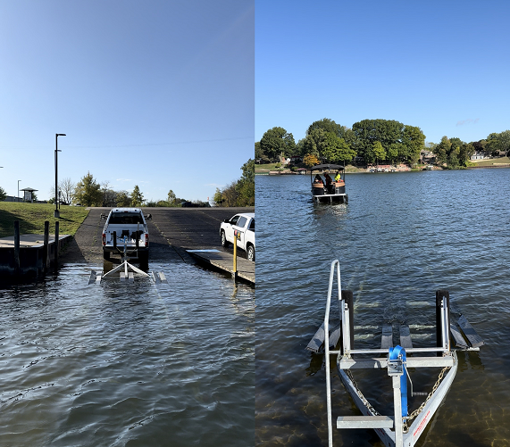
Figure 1: Motivation scenario: automatic loading of a pontoon boat to a trailer.

I-A Related works

The automated docking of autonomous surface vehicles has been widely studied over decades, while it is more recent that an increasing volume of new literature has been observed along with comprehensive survey papers [li2020survey, qiang2022review, simonlexau2023automated, choi2023review].

In particular, the authors of [mizuno2015quasi] formulated nonlinear programming for minimal berthing time. They showed the effectiveness of non-linear programming with hydrodynamics along with disturbance – while the disturbances considered to be fixed for a period of minutes, which might not be realistic. The authors in [martinsen2019autonomous] additionally introduced a convex set for a spatial constraint of collision avoidance and directly applied the optimal solutions for control. The authors further improved their work in [bitar2020trajectory] by adding a lower-level control to address disturbances and model errors. The work was shown effective with a real-size passenger ferry called milliAmpere which is comparable (5 by 2.8 [m]) in size with our vehicle (8.36 by 3.1 [m]). Although we are motivated by the study [bitar2020trajectory], we further explore the potential of direct control where we directly consider real-time wind disturbances in our non-linear programming without having a downstream controller to address disturbances. Also, none of the existing studies solve the “trailer loading” problem which requires additional constraints, accuracy, and precision.

Trajectory planning and control with wind disturbance is a common challenge in aerial applications [cole2018reactive, cole2019trajectory]. Wind disturbances are typically considered an additive force to the system dynamics, and the resulting trajectory planning is shown effective against the wind effect – and we adopt the intuition in this work.

While not exactly aligned, some studies have motivated our system designs. The authors in [wang2022motion] formulate the trailer loading problem for a truck, introducing a useful insight of linearly extending a hitching point to ensure alignment in angles from distance. The authors in [knizhnik2021docking] propose a docking/undocking control of a swimming robot, with discrete strategies of retrials – which we redesigned as a bail strategy.

Overall, despite the increasing body of literature, there is a lack of studies on automated docking and loading to trailers, which can be widely received by broader audiences (including industries). Thus we add the following three contributions to the literature: First, we construct a complete system pipeline for automated trailer loading of a surface vehicle. The pipeline includes localization/perception, system identification for the test boat, reference path planning, and trajectory optimization. Second, we propose extensions to enhance the reliability of maneuvers that are readily applicable in practice, without adding complexity. Lastly, we report the demonstration results with a commercial boat (Premier Intrigue) conducted in Michigan in October 2023, which can serve as a valuable reference.

The remainder of the paper is structured as follows. Section II formalizes the problem setting in this study. In Section III, our localization and perception systems are discussed. Section IV shows the trajectory optimization method, followed by Section V showing the extensions to make the trajectory more reliable. Section LABEL:sec:experiments discusses the experiment results. Section LABEL:sec:conclusions concludes the paper with a summary and future work.

II Problem Settings

II-A Target scenario

Figure 1 represents our target scenario, where a trailer is fixed in position and angles. The automated docking system is activated from a distance with a variable pose. Different initial distances have been explored as a starting point.

Figure 2: Test boat: Premier Intrigue of 2022 model year. Specifications are with overall length of 8.36 [m], beam length of 3.1 [m], and dry weight of 3,500 [lb].

II-B System Pipeline

Figure 3 illustrates the pipeline of the system that includes: (i) perception, (ii) localization, (iii) reference path planning, and (iv) trajectory generations. Note that the current pipeline does not include “feedback” controller, leaving the control strategy feedforward. The feedback controller will presumably enhance the performance by compensating for system errors or other unknown disturbances/randomness; this work showcases the effectiveness of the system identification and resulting trajectory planning such that the feedforward approach can work effectively on its own. It is still essential to note that a combination of feedforward and feedback controller, being a hybrid method, may offer the best performance, which is a natural extension of this work.

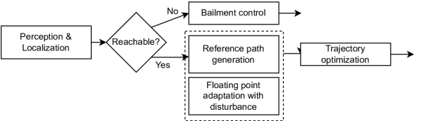
Figure 3: System pipeline, consisting of localization, reference path generation, and trajectory planning. There exists an intermittent condition to necessitate a bail strategy (in case docking is not feasible).

II-C System Dynamics and Estimation

For notational convenience, vector terms are in bold and matrix terms are additionally capitalized. Using Fossen’s model based on maneuvering theory [fossen2011handbook], the USV dynamics with wind disturbances (excluding current and wave forces) are written in vector-form as:

$$\dot{\mathbf{\eta}} =\mathbf{R}(\psi)\mathbf{v},$$ (1)

$$\textbf{M}\dot{\textbf{v}}+\textbf{C}(\textbf{v})\textbf{v}+\textbf{D}(\textbf{v})\textbf{v} =\bm{\tau}_{\text{prop}}+\bm{\tau}_{\text{wind}}+\bm{\tau}_{\text{wave}},$$ (2)

where ${\mathbf{\eta}}=[x~{}y~{}r]^{T}$ is the pose vector and $\textbf{v}=[u~{}v~{}r]^{\top}$, is the vector of the vehicle’s surge velocity, sway velocity, and yaw rate in the body fixed frame. M represents the inertia matrix, $\textbf{C}(\textbf{v})$ denotes Coriolis-centripetal forces, and $\textbf{D}(\textbf{v})$ relates to the hydrodynamic damping forces acting on the hull. Both M and $\textbf{C}(\textbf{v})$ are a combination of rigid body and added mass components. $\textbf{D}(\textbf{v})$ contains both linear viscous damping and nonlinear damping terms, based on cross-flow drag theory and second-order modulus functions [fossen2011handbook]. Using symmetry considerations, they can be simplified and represented in a parametric manner as follows [pedersen2019optimization]:

$$\textbf{M}:=\begin{bmatrix}m_{11}&0&0\\ 0&m_{22}&m_{23}\\ 0&m_{32}&m_{33}\\ \end{bmatrix}$$ (3)

$$\textbf{C}(\textbf{v})=\begin{bmatrix}0&0&c_{13}(\textbf{v})\\ 0&0&c_{23}(\textbf{v})\\ -c_{13}(\textbf{v})&-c_{23}(\textbf{v})&0\end{bmatrix}$$ (4)

where $c_{13}(\textbf{v})=-m_{22}v-m_{23}r$ and $c_{23}(\textbf{v})=m_{11}u$.

$$\textbf{D}(\textbf{v}):=\begin{bmatrix}d_{11}(\textbf{v})&0&0\\ 0&d_{22}(\textbf{v})&d_{23}(\textbf{v})\\ 0&d_{32}(\textbf{v})&d_{33}(\textbf{v})\end{bmatrix}$$ (5)

where $d_{11}(\textbf{v})=-X_{u}-X_{|u|u}|u|$, $d_{22}(\textbf{v})=-Y_{v}-Y_{|v|v}|v|$, $d_{23}(\textbf{v})=-Y_{r}$, $d_{32}(\textbf{v})=-N_{v}-N_{|v|v}|v|$, and $d_{33}(\textbf{v})=-N_{r}-N_{|r|r}|r|$.

A thorough system identification procedure was performed to determine the appropriate parameters that corresponded to the dynamics of the ship hull considered in this application. Data was collected on the boat in a diverse range of velocity profiles while performing maneuvers such as turning, zigzag, and straight lines in both forward and reverse motion [eriksen2017modeling]. Given the under-actuated nature of the boat, surge dynamics was decoupled from the sway and yaw rate dynamics to facilitate parameter identification. Steady-state data was substituted into the resulting equations and a least-squares regression analysis using the Pseudo inverse [woo2018dynamic] led to the estimated parameter values listed below in Table I.

In addition, the boat propulsion forces ${\tau}_{\text{prop}}\in\mathrm{R}^{3\times 1}$ were modeled as $\tau_{\text{prop}}:=[\tau_{X}~{}\tau_{Y}~{}\tau_{N}]$, where $\tau_{X}=F\cos\alpha_{1}+F\cos\alpha_{2}$, $\tau_{Y}=F\sin\alpha_{1}+F\sin\alpha_{1}$, and $\tau_{N}=F(-L_{x}\sin\alpha_{1}-L_{y}\cos\alpha_{1})+F(-L_{x}\sin\alpha_{2}+L_{y}\cos\alpha_{2})$. Here, $\alpha$ denotes the azimuth angle of the thrusters and $F$ represents the thrust force generated by them. The engine and propeller were initially modeled in CAD. A propeller open water (POW) test was conducted using Computational Fluid Dynamics (CFD) tools to determine how much thrust would be generated by propeller rotation. For a given configuration, the thrust force ($F$) generated by both engines is assumed to be the same, and can be determined as a function of the propeller RPM using the following equation

$$F=\rho K_{T}D^{4}|n|n,$$ (6)

where $\rho$ refers to the density of water, $K_{T}$ is the propulsion coefficient obtained from the POW test, $D$ is the propeller diameter, and $n$ is the propeller RPM. $n$ is negative when the engine transmission is in reverse gear. Discrepancies between the RPMs of the starboard and port engines are considered to be minimal.

TABLE I: Parameters from System Identification

Parameters	Values	Parameters	Values
$m_{11}$	$5251.26\,[{kg}]$	$Y_{vv}$	$-1958.61\,[\frac{kg}{s}]$
$m_{22}$	$4077.23\,[{kg}]$	$Y_{r}$	$-1121.8\,[\frac{kg}{s}]$
$m_{23}$	$13.29\,[{kg}]$	$N_{r}$	$-14208.2\,[\frac{kg}{s}]$
$m_{32}$	$1251.01\,[{kg}]$	$N_{rr}$	$-53206.72\,[\frac{kg}{s}$]
$m_{33}$	$16373\,[{kg{m}^{2}}]$	$N_{v}$	$-2300\,[\frac{kg}{s}]$
$X_{u}$	$-40\,[\frac{kg}{s}]$	$N_{vv}$	$3190.9\,[\frac{kg}{s}]$
$X_{uu}$	$-288.8\,[\frac{kg}{s}]$	$\rho$	$998.12\,[\frac{kg}{m^{3}}]$
$Y_{v}$	$-2159.93\,[\frac{kg}{s}]$	$K_{T}$	$0.44[\frac{1}{s^{2}}]$

Furthermore, as described in [fossen2011handbook], wind forces and moments induced in a 3DOF moving marine vessel are based on the projected area of the ship and the relative wind velocities.

$$\tau_{\text{wind}}=q_{a}\begin{bmatrix}C_{X}(\gamma_{rw})A_{Fw}\\ C_{Y}(\gamma_{rw})A_{Lw}\\ C_{N}(\gamma_{rw})A_{Lw}L_{oa}\\ \end{bmatrix}$$ (7)

where the dynamic wind pressure $q_{a}=\frac{1}{2}\rho_{a,T}V_{rw}^{2}$ is directly proportional to the mass density of air $\rho_{a,T}$ at a given temperature and $V_{rw}$ is the relative mean wind speed. $\gamma_{rw}$ represents the wind direction relative to the vessel and the wind coefficients $C_{X}(\gamma_{rw})$, $C_{Y}(\gamma_{rw})$, and $C_{N}(\gamma_{rw})$ are numerically computed based on historical data for different types of vessels [blendermann1994parameter]. Since the trailer loading application occurs near the shore, the impacts of wave forces ($\tau_{\text{wave}}$) and any other current forces are neglected in this investigation.

II-D Reference Path

We leverage the well-adopted Dubin’s path algorithm [dubins1957curves] for its computational efficiency and capability of constraining a curvature limit in the applications of underactuated systems.

III Localization System

III-A Target level of Accuracy

The trailer typically provides a 30 [cm] clearance for the pontoon hull to enter, which demands precise and accurate positioning. Furthermore, the loading area of the trailer is typically shared by others (skippers and boats), so failure to accurately position the vehicle may result in causalities and damage to the boats. However, the target level of accuracy is yet to be explored, given the absence of prior work that resembles this application. We consult with research in the field of automated ground vehicles [tyler2019requirement] and apply it by adjusting the parameters: the allowable probability of failure per hour (to 32% that corresponds to a 1-sigma level of confidence) and the geometry to represent the boat and trailer. Consequently, the obtained target level of accuracy is tabulated in Table II.

TABLE II: localization accuracy requirement for 68% of probability of success per hour.

	0-23 [m]	23-36 [m]	36 [m] or beyond
$\delta\psi$ [deg]	3	3	3
$\delta_{\text{lateral}}$ [m]	0.37	1.33	2.90
$\delta_{\text{longitudinal}}$ [m]	0.67	2.14	3.58

III-B Applied Methods to Enhance Accuracy

As trailer loading takes place in an outdoor environment, it is susceptible to varying illumination conditions influenced by weather and time of day. To address this challenge, we opted for a camera equipped with High Dynamic Range (HDR) capabilities. However, the camera has a frequency of 6.9 [FPS] which is insufficient for the system frequency, 10 [Hz]. Thus we employed a Kalman Filter to synchronize the frequency, which also helps smooth out noises.

Another challenge is aligned with the trailer leveling the ramp underwater (such that the boat hitches on top), being not visible from the camera. To avoid this, we used a passive tag (AprilTag [olson2011tags]) for its accuracy and robustness in its performance.

III-C Resulting Sensor Configuration

Along with the applied methods in the previous section, our final sensor configuration consists of: a RTK/AHRS sensor, a GNSS/INS sensor, and a camera. The localization process follows: (i) At the beginning of the experiment, the trailer’s initial point is inferred utilizing RTK and AHRS sensors; (ii) A GNSS/INS sensor estimates the relative position of the ego boat to the trailer; (iii) A camera provides a reference to add accuracy. Note that we solely rely on GPS and IMU data (i.e., from GNSS/INS) beyond the camera’s range of detecting the AprilTag.

III-D Performance

Figure 5 shows the performance of the localization based on camera images against RTK (representing ground truth). It should be noted that the relative pose error decreases linearly as the boat gets closer to the trailer after the camera detects the tag around 60 [m] from the trailer. Also, the Kalman filter (denoted as KF in Fig. 5) effectively smooths out relative headings. Overall, the localization performance was measured as: 0.58 [m] of average offset in longitudinal, 0.26 [m] in lateral, and 2.3 [deg] in heading for the range of 0-23 [m] from the trailer – this suggests that the implemented localization system is successfully meeting the target in Table II.

Figure 4: The camera installed at the bow of the pontoon. Specifications: 2880x1860 of resolution, 6.9 [FPS], 8 [mm] of focal length, 58.4 [deg] of FOV.

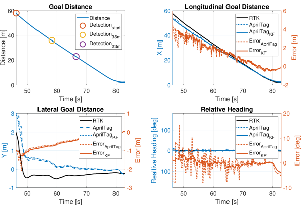
Figure 5: Performance of the localization based on the camera images against RTK. Top left: distance of the goal position from the ego vehicle. Circles represent some examples of detection at distance (23, 36, 60 [m]). Top right: longitudinal target distance and its error in an ego-centric frame. Bottom left: lateral target distance and its error in the ego-centric frame. Bottom right: relative heading of the trailer in the ego-centric frame and its error. Note that the camera starts to detect within 60 [m] from the tag, which occurs around 45 [sec] in the time axis.

IV Trajectory Optimization

IV-A Objective

The objective is to optimize the trajectory to a docking point with minimum control effort and deviation from the reference trajectory while ensuring the marine craft is oriented according to the docking point. The speed is also optimized so that the boat approaches the docking point smoothly. The states are $\textbf{s}(t)=[x(t),y(t),\psi(t),u(t),v(t),r(t)]^{\top}\;\forall t\in\{0,1,\cdots,T\}$ and the control variables are $\textbf{c}(t)=[n(t),\alpha(t)]^{\top}\;\forall t\in\{0,1,\cdots,T-1\}$. As mentioned above, $n(t)$ refers to the RPM of the propeller and $\alpha(t)$ indicates the azimuth (or steering) angle of the engines.

The objective function reads:

$$J=\sum_{t=0}^{T-1}\textbf{c}^{T}(t)\,{\Lambda}_{\tau}\,\textbf{c}(t)+\delta\textbf{s}^{T}(t)\,{\Lambda}_{\text{ref}}\,\delta\textbf{s}(t)$$ (8)

where the first term penalizes control efforts and the second term penalizes the deviation from the reference trajectory $\delta\textbf{s}(t)=[\textbf{s}(t)-\textbf{s}_{\text{ref}}(t)]\;\forall t\in\{0,1,\cdots,T\}$. The matrices $\Lambda_{\tau}$ and $\Lambda_{\text{ref}}$ are the corresponding penalty weights in the control effort and deviation from the reference path, respectively.

Remark 1

The objective function can leverage different penalty designs such as pseudo-Huber functions as presented in [bitar2020trajectory] to apply quadratic penalties to minor errors while employing linear penalties for more significant errors – that helps avoid the large position errors dominating the cost evaluations.

IV-B Constraints

The constraints represent: (i) vehicle dynamics, (ii) control bounds, (iii) initial conditions, and (iv) terminal conditions, in particular, the heading angle that matches the docking angle. Formally:

$$\textbf{s}(t+1) =f(\textbf{s}(t),\textbf{c}(t))\;\forall\,t\in\{0,1,\cdots,T-1\},$$ (9)

$$\textbf{c}_{\text{min}} \leq\textbf{c}(t)\leq\textbf{c}_{\text{max}}\;\forall\,t\in\{0,1,\cdots,T-1\},$$ (10)

$$\textbf{s}(0) =\textbf{s}_{0},$$ (11)

$$\psi(T) =\psi_{d},$$ (12)

where $\textbf{s}_{0}$ is the measured state at time $t=0$, i.e., initial state, and $\psi_{d}$ is the docking angle. Note that the constraint on the angle of the docking (12) is only applied when the docking point is within the planning horizon (in time). Alternatively, it can be added to the objective function as a soft constraint to ensure feasibility.

The discrete-time dynamics (9) is obtained from a first-order Euler discretization of Fossen’s equations (2).

IV-C Complete optimization problem

The complete optimization problem now reads:

$$\min_{s,c}\;\eqref{eq:obj}$$

subject to: $$\eqref{const:dynamics}-\eqref{const:docking_angle}.$$ (13)

The optimization can be solved by nonlinear programming (with the nonlinearity in the dynamics (9)). Although the optimization problem in (13) is theoretically rigorous, we need further extensions for a reliable and successful maneuver in practice, along with measurement noise, dynamically changing environment, and latencies. Section V details it.

V Extensions

We introduce the technical extensions for trajectory optimizations to enhance reliability and safety.

V-A Extended Docking Point

In busy hours, the docking area can be crowded with other marine crafts, so it is often necessary to have minimal steering to ensure safety when the dock is close. An associated strategy is to align the boat with the trailer from a distance and approach straight, motivated by [wang2022motion]. This strategy is integrated into our planner by setting a virtual docking point that is straightened from the actual docking point. The reference path in Section II-D utilizes the extended docking point as the target. The final reference path thus guarantees a straight pivoting from a distance.

V-B A floating reference point instead of the path

There are two practical challenges in directly applying the reference path generated in Section II-D. First, it does not consider dynamics, momentum, or disturbances. Therefore, there exists a model mismatch between the reference path and the trajectory generated by the motion planner. Second, the reference path is integrated into (8) at each time step, indicating the necessity of temporal mapping of the reference path. A speed profile can be precomputed along with the reference path; however, the reference speed profile does not account for the dynamics either, and the resulting profile may not be optimal for motion planning. Thus, we generate a “floating reference point” that is set to static for each planning horizon. The reference point is “floated” against the wind direction such that the motion planner can offset the disturbances. The reference point is selected as a lookahead point (that is N meters away from the ego boat) within the reference path. The reference point is shifted toward the opposite direction of the wind with a scalar that corresponds to the speed of the wind.