Computing almost commuting bases of ODOs
and Gelfand-Dikey hierarchies

Abstract

Almost commuting operators were introduced in 1985 by George Wilson to present generalizations the Korteweg-de Vries hierarchy, nowadays known as Gelfand-Dikey (GD) hierarchies. In this paper, we review the formal construction of the vector space of almost commuting operators with a given ordinary differential operator (ODO), with the ultimate goal of obtaining a basis by computational routines, using the language of differential polynomials. We use Wilson’s results on weigheted ODOs to guarantee the solvability of the triangular system that allows to compute the homogeneous almost commuting operator of a given order in the ring of ODOs. As a consequence the computation of the equations of the GD hierarchies is obtained without using pseudo-differential operators. The algorithms to calculate the almost commuting basis and the GD hierarchies in the ring of ODOs are implemented in SageMath, and explicit examples are provided.

MSC[2020]: 13N10, 13P15, 12H05

1 Introduction

Almost commuting operators were introduced in 1985 by George Wilson in [20] to present the Lax representations and generalizations of the Korteweg-de Vries hierarchy, nowadays known as the Gelfand-Dikey (GD) hierarchies [5, 6]. The generalization of the Korteweg-de Vries hierarchy, passing from a second-order linear differential operator to an $n$-th order operator $L$ was suggested by Krichever, Gelfand and Dickey, see references in [5, 6]. The standard construction of these generalized hierarchies is based on fractional powers $L^{m/n}$ of an operator $L$ of order $n$, which live in a ring of pseudo-differential operators.

The question addressed is this paper is the design of a symbolic algorithm that allows the computation of the GD hierarchies but does not require computations with pseudo-differential operators. We develop an algorithm that requires computations in a ring of differential operators $\mathcal{D}$ whose coefficients belong to a ring of differential polynomials. This is possible by the notion of almost commuting operator defined by G. Wilson in  [21], as an operator $A\in\mathcal{D}$ such that $[L,A]=LA-LA$ has order $\leq n-2$. We reorganized previously known ideas (by Wilson and many others) to prove that the vector space $W(L)$ of almost commuting operators with a given ordinary differential operator $L$

$$W(L)=\{A\in\mathcal{D}\mid\rm ord[L,A]\leq n-2\}=Z((L))_{+}.$$

equals the set $Z((L))_{+}$ of positive parts of the elements of the centralizer $Z((L))$ of $L$ in the ring of pseudo-differential operators, see Theorem 3.5.

Our motivation comes from the need of having a basis of almost commuting operators, and explicit formulas for integrable hierarchies, to determine differential operators with nontrivial centralizers. Hence our ultimate goal is to obtain such bases by computational routines. We saw in the work of Grunbaum [8] the possibility of developing symbolic algorithms. We used preliminary implementations of these algorithms in Maple to compute the examples in previous works of some of the authors, see [13, 15], and [16]. We need meaningfulexamples of prime order ODOs to extend the results in [16], and then develop a suitable Picard-Vessiot theory for spectral problems.

Considering a set $U=\{u_{2},\ldots,u_{n}\}$ of differential variables over the field of rational numbers $\mathbb{Q}$, with respect to a given derivation $\partial$, we aim to compute a basis of $W(L)$ for the formal differential operator

$$L=\partial^{n}+u_{2}\partial^{n-2}+\ldots+u_{n-1}\partial+u_{n}.$$ (1)

Wilson defined a weight function on the ring of differential polynomials $\mathcal{R}=\mathbb{Q}\{U\}$, that guaranteed the existence of a unique basis $\mathcal{H}(L)=\{P_{m}\mid m\in\mathbb{N}\}$ whose operators are homogeneous with respect to the weight function. A natural approach to seek for an homogeneous almost commuting operator $P_{m}$ of order $m$ is to define the formal operator

$$\tilde{P}_{m}=\partial^{m}+y_{2}\partial^{m-2}+\ldots+y_{m-1}\partial+y_{m}$$

whose coefficients are differential variables in $Y=\{y_{2},\ldots,y_{m}\}$ with respect to $\partial$, and force $[L,\tilde{P}_{m}]$ to be a differential operator of order $\leq n-2$. This produces a differential system $\mathbb{E}_{m,n}$ of $m-2$ equations given by differential polynomials in $\mathbb{Q}\{U,Y\}$. We proved that $\mathbb{E}_{m,n}$ is a triangular system w.r.t. the variables $Y$ in Theorem 4.5 and moreover that

$$\mathbb{E}_{m,n}=\{y^{\prime}_{i}+e_{i}(Y)=0\mid i=2,\ldots m\}$$

where $e_{2}\in\mathbb{Q}\{U\}$ and

$$e_{i}(Y)\in\mathbb{Q}\{U\}\{y_{2},\ldots,y_{i-1}\},\,\,\,i\geq 3$$

are differential polynomials, homogeneous with respect to an extended weight function on $\mathbb{Q}\{U,Y\}$. We use Wilson’s results on weigheted ODOs to guarantee the solvability of this triangular system, that allows to compute a unique solution set $Z$ of $\mathbb{E}_{m,n}$ w.r.t. $Y$. We can solve $\mathbb{E}_{m,n}$ by using the integration methods for differential polynomials described in  [1] and  [2], combined with backwards substitution.

Replacing each variable in $Y$ by the corresponding solution in $Z$, the almost commuting operator $P_{m}$ is obtained together with the commutator

$${[P_{m},L]}=H_{m,0}+H_{m,1}\partial+\cdots+H_{m,n-2}\partial^{n-2},$$

where $H_{m,k}(U)$, $k=0,\ldots,n-2$ are the differential polynomials in $\mathbb{Q}\{U\}$ that determine the GD hierarchies as being defined in [5, 6, 21].

The algorithms to compute the almost commuting basis and the GD hierarchies, in the ring of ODOs are implemented in the SageMath package dalgebra [9, 19]. More details of this implementation and of the computations performed are included in Section 6.

The paper is organised as follows. In Section 2 we provide all the formal definitions for the differential algebra concepts that are used throughout the paper. We recall in Section 3 the main structural result of Wilson for almost commuting operators. In Section 4 we will show the direct method for computing almost commuting bases. First we will present how to obtain a triangular differential system for solving this differential system. We proceed to show in Section 5 how this method produces the first elements on the GD hierarchies for an operator $L$ of order 3 and 5. Finally, Section 6 contains a description of the software implemented in SageMath [19], and the results obtained with our symbolic algorithms.

2 Preliminaries

A differential ring $(R,\partial)$ is a ring $R$ (assumed associative, with identity) equipped with a specified derivation $\partial$, that is, an additive map $\partial:R\rightarrow R$ satisfying the product rule: $\partial(xy)=\partial(x)y+x\partial(y)$ for all $x,y\in R$. The elements $r\in R$ such that $\partial(r)=0$ are called constants of $R$, and the collection of these constants forms a subring of $R$. A differential field $(K,\partial)$ is a differential ring which is a field.

For concepts in differential algebra, related with differential polynomials, we refer to [10, 14]. Let $\mathbb{N}$ be the set of positive integers including zero. Given a differential variable $y$ with respect to $R$, we define $y^{(i)}$ as $\partial^{i}(y)$, for $y\in\mathbb{N}$, $i\geq 1$ and $y^{(0)}$ as $y$. The ring of differential polynomials over $R$ in the differential variable $y$ is the polynomial ring

$$R\{y\}=R[y^{(i)}\mid i\in\mathbb{N}].$$

The notation $y^{\prime}$, $y^{\prime\prime}$, $y^{\prime\prime\prime}$ will be also used for $y^{(i)}$, $i=1,2,3$. Observe that $R\{y\}$ is also a differential ring with the natural extended derivation, that we also call $\partial$ abusing notation. We can iterate this construction, adding several differential variables. Given differential variables $y$ and $z$ over $R$, the ring of differential polynomials in $y$ and $z$ is denoted by $R\{y,z\}$ and defined as $R\{y\}\{z\}\simeq R\{z\}\{y\}$.

A differential ring $(R,\partial)$, defines a ring of (linear) differential operators $R[\partial]$, which is a non commutative ring, where the multiplication of two elements of is the composition of the two differential operators, defined by the rule $\partial r=\partial(r)+r\partial$ for all $r\in R$. It is an Ore polynomial ring [7]. A differential operator $A\in R[\partial]$ can be written in a unique way as

$$A=a_{n}\partial^{n}+a_{n-1}\partial^{n-1}+\ldots+a_{1}\partial+a_{0},\mbox{ with }a_{i}\in R,\,\,\,\mbox{ with }a_{n}\neq 0.$$

Then the order of $A$ is $n$, denoted $\rm ord(A)=n$, with the convention $\rm ord(0)=-\infty$. This order has the same property as the degree of a polynomial: the order of a product is the sum of the orders and the order of a sum is bounded by the maximal order of the summands. The coefficient of the highest order term of $A$ is the leading coefficient of $A$, denoted $\operatorname{lc}(A)=a_{n}$. We say that an operator $A\in R[\partial]$ of order $n$ is in normal form if it is monic, i.e., it has $\operatorname{lc}(A)=1$, and the coefficient of the order $n-1$ term is zero, namely,

$$A=\partial^{n}+a_{n-2}\partial^{n-2}+\ldots+a_{1}\partial+a_{0}.$$

In [12, 22] these operators are called elliptic operators. Differential operators with coefficients in a differential field can be always brought to normal form, by using a change of variable and conjugation by a function, which are the only two possible automorphisms.

Let us assume that the ring of constants of $R$ is a field $\mathbf{C}$ of zero characteristic. Since $R[\partial]$ is a non-commutative ring, we can define the corresponding Lie-bracket over $R[\partial]$ as a $\mathbf{C}$-bilinear map $[\cdot,\cdot]$ defined by

$$[A,B]=AB-BA.$$

It is clear that $A$ and $B$ commutes if and only if $[A,B]=0$. We also say that $[A,B]$ is the commutator of $A$ and $B$. We define the centralizer of $A$ in $R[\partial]$ as

$$\mathcal{Z}(A)=\{B\in R[\partial]\ :\ [A,B]=0\}.$$

Since $[\cdot,\cdot]$ is a $\mathbf{C}$-bilinear map, then $\mathcal{Z}(A)$ is a $\mathbf{C}$-module.

Lemma 2.1.

Let $A,B$ be two differential operators in $R[\partial]$ of orders $n$ and $m$ respectively. Then $\rm ord([A,B])\leq n+m-1$. If $A$ and $B$ are both in normal form, then $\rm ord([A,B])\leq n+m-3$.

Proof.

Since $\operatorname{lc}(AB)=\operatorname{lc}(A)\operatorname{lc}(B)=\operatorname{lc}(BA)$, we have that the term of order $n+m$ of $[A,B]$ is always zero, implying $\rm ord([A,B])\leq n+m-1$. Moreover, if $A$ and $B$ are in normal form, we can write $A=\partial^{n}+\tilde{A}$ and $B=\partial^{m}+\tilde{B}$ where $\tilde{A}$ and $\tilde{B}$ have orders bounded by $n-2$ and $m-2$ respectively. Then

$$[A,B]=[\partial^{n},\partial^{m}]+[\tilde{A},\partial^{m}]+[\partial^{n},\tilde{B}]+[\tilde{A},\tilde{B}].$$

The first bracket always vanishes and the orders of the other three brackets are bounded by $n+m-3$. ∎

Let us denote by $R((\partial^{-1}))$ the ring of pseudo-differential operators in $\partial$ with coefficients in the differential ring $R$, defined as in [7]

$$R((\partial^{-1}))=\left\{\sum_{i=-\infty}^{n}a_{i}\partial^{i}\mid a_{i}\in R,n\in\mathbb{Z}\right\},$$

where $\partial^{-1}$ is the inverse of $\partial$ in $R((\partial^{-1}))$, $\partial^{-1}\partial=\partial\partial^{-1}=1$, and it satisfies the following commutation rule with elements $r\in R$

$$\partial^{-1}r=\sum_{i=1}^{\infty}(-1)^{i-1}\partial^{i-1}(r)\;\partial^{-i}\ .$$

Observe that

$$\mathcal{Z}(L)\subset R[\partial]\subset R((\partial^{-1})).$$

Given $A=\sum_{i=-\infty}^{n}a_{i}\partial^{i}$, with $a_{n}\neq 0$ then $n$ is called the order of $A$, denoted by $\rm ord(A)$ and $a_{n}$ is called the leading coefficient of $A$. We define the positive part of $A$ as the differential operator

$$A_{+}=\sum_{i=0}^{n}a_{i}\partial^{i}\in R[\partial]\ \textrm{ if }n\geq 0\ ,\ \textrm{ and }A_{+}=0\ \textrm{ otherwise }.$$ (2)

We denote by $A_{-}=A-A_{+}$. Given $A,B\in R((\partial^{-1}))$ of orders $m$ and $n$ respectively, we can also define their commutator $[A,B]$. Using the natural decomposition $A=A_{+}+A_{-}$, we can see that

$$[A,B]=[A_{+},B_{+}]+[A_{-},B_{+}]+[A_{+},B_{-}]+[A_{-},B_{-}],$$

which easily proves that Lemma 2.1 extends to pseudo-differential operators, see for instance [7].

3 Almost Commuting Operators

Let us consider a differential ring $(R,\partial)$ whose ring of constants $\mathbf{C}$ is a field of zero characteristic.

Given a monic $n$-th order differential operator $L$ in $R[\partial]$, it is well known that it has a unique monic $n$-th root, denoted by $L^{1/n}$, see for instance [7, Proposition 2.7]. In addition, $L^{1/n}$ determines the centralizer in $R((\partial^{-1}))$ of $L$, denoted by $\mathcal{Z}((L))$ and equal to

$$\mathcal{Z}((L))=\left\{\sum_{j=-\infty}^{m}c_{j}(L^{1/n})^{j}\mid c_{j}\in{\bf C},m\in\mathbb{Z}\right\},$$ (3)

by [7, Theorem 3.1]. This implies that $\mathcal{Z}((L))$ is commutative. This result is a generalization of a famous theorem by I. Schur in [17], originally stated for analytic coefficients, to differential operators with coefficients in a differential ring $R$. This theorem has a long history, see for instance [7, Sections 3 and 4], and the references therein.

An immediate consequence of (3), given in the next lemma, motivates the definition of almost commuting operators, originally introduced by G. Wilson in [18, 21]. Let us consider the set $\mathcal{Z}((L))_{+}$ of all positive parts of the pseudo differential operators in $\mathcal{Z}((L))$, that is

$$\mathcal{Z}((L))_{+}:=\{A_{+}\mid A\in\mathcal{Z}((L))\}.$$ (4)

Observe that $\mathcal{Z}((L))_{+}$ is a $\mathbf{C}$-linear space.

Lemma 3.1.

Let us consider a monic differential operator $L\in R[\partial]$ of order $n$. For every $A\in\mathcal{Z}((L))_{+}$ it holds that $\rm ord([L,A])\leq n-2$.

Proof.

Given $B\in\mathcal{Z}((L))$. Let us consider the natural decomposition $B=B_{+}+B_{-}$ and observe that $B_{-}$ is a pseudo differential operator of order at most $-1$. Since $B\in\mathcal{Z}((L))$ then $0=[L,B]=[L,B_{+}]+[L,B_{-}]$ implying that the order of $[L,B_{+}]$ equals the order of $[L,B_{-}]$. This order is less than or equal to $n-2$. ∎

The next definition is naturally motivated by the previous lemma.

Definition 3.2 ([21]).

Let $L\in R[\partial]$ be a differential operator of order $n$. We say that $A\in R[\partial]$ almost commutes with $L$ if $\rm ord([L,A])\leq n-2$. We denote by $W(L)$ the set of all differential operators that almost commute with $L$.

Lemma 3.3.

Let $(R,\partial)$ be a differential ring, whose ring of constants is a field $\mathbf{C}$ of zero characteristic. Given a differential operator $L\in R[\partial]$ the following statements hold.

1. $W(L)$ is a $\mathbf{C}$-vector space.

2. Given $A\in W(L)$ then $\operatorname{lc}(A)\in\mathbf{C}$.

Proof.

For every $B_{1},B_{2}\in W(L)$ and $c\in\mathbf{C}$ using the $\mathbf{C}$-linearity of the Lie bracket:

$$[L,cB_{1}+B_{2}]=c[L,B_{1}]+[L,B_{2}].$$

Thus, it is clear, by the properties of the order, that $cB_{1}+B_{2}\in W(L)$ again, proving the first statement.

Given $A\in W(L)$, let us prove that $\operatorname{lc}(A)$ is a constant. If $\rm ord(A)=m$, let $a_{m}=\operatorname{lc}(A)$ and it is easily proved that the leading term of $[L,A]$ is $na_{m}^{\prime}\partial^{n+m-1}$. Since $\rm ord([L,A])\leq n-2$ then $a_{m}^{\prime}=0$, proving that $a_{m}\in\mathbf{C}$. ∎

Lemma 3.1 implies that $\mathcal{Z}((L))_{+}\subseteq W(L)$. We will prove next that equality holds. Given an $n$-th root $L^{1/n}$ of $L$ we denote its $m$-th power by $L^{m/n}$.

Proposition 3.4.

Let us consider a monic differential operator $L\in R[\partial]$ of order $n$ and choose an $n$-th root $L^{1/n}$ of $L$. Then the set $\mathcal{B}(L)=\{B_{j}=(L^{j/n})_{+}\mid j\in\mathbb{N}\}$ is a basis of $\mathcal{Z}((L))_{+}$ as a $\mathbf{C}$-vector space.

Proof.

The existence of $B=L^{1/n}$ is guarantied by [7], Proposition 2.7. Note that $B$ has order one. Thus $B_{0}=1$ and $\rm ord(B_{j})=j$, for every $j\in\mathbb{N}\backslash\{0\}$. Thus $\mathcal{B}(L)$ is a set of linearly independent differential operators and, by (4) and (3), it is a generating set of $\mathcal{Z}((L))_{+}$ as a $\mathbf{C}$-vector space. ∎

Theorem 3.5.

Let $L\in R[\partial]$ be monic. Then $\mathcal{Z}((L))_{+}=W(L)$.

Proof.

Assuming that $L$ has order $n$, we consider the $\mathbf{C}$-basis $\mathcal{B}(L)=\{B_{j}=(L^{j/n})_{+}\mid j\in\mathbb{N}\}$ of $\mathcal{Z}((L))_{+}$ as in Proposition 3.4. By Lemma 3.3, given $A\in W(L)$ of order $m$ then there exists $c_{m}\in\mathbf{C}$ such that $A-c_{m}B_{m}$ belongs to $W(L)$ and has order less than or equal to $m-1$. Now by induction on the order of $A$, we conclude that $A\in\mathcal{Z}((L))_{+}$. ∎

3.1 Formal differential operators

Let us consider a set $U=\{u_{2},\ldots u_{n}\}$ of differential variables with respect to a derivation $\partial$ and the ring of differential polynomials $\mathcal{R}=\mathbf{C}\{U\}$, with the extended derivation

$$\partial^{q}(u_{\ell})=u_{\ell}^{(q)},\quad q=1,2,\dots.$$ (5)

Then $\mathcal{R}$ is a differential ring whose ring of constants equals the $\mathbf{C}$. We call $\mathcal{R}[\partial]$ the ring of formal differential operators in the differential variables $U$ and its elements formal differential operators.

Weight function. We define a weight function $w$ over $\mathcal{R}$ given by $w(u_{\ell})=\ell$, and

$$w(u_{\ell}^{(k)})=\ell+q,\ k=1,2,\dots.$$ (6)

As in [18, Proposition 4.2], we call an operator $P\in\mathcal{R}[\partial]$ homogeneous of weight $r$ with respect to $w$ if the coefficient of $\partial^{i}$ in $P$ has weight $r-i$. This is equivalent to extending $w$ to $\mathcal{R}[\partial]$ by setting $w(\partial)=1$. From the homogeneity of the commutation rule $\partial p=p\partial+\partial(p)$, for every $p\in\mathcal{R}$ it follows that the product of two operators that are homogeneous of weights $r$ and $s$ is homogeneous of weight $r+s$.

Let $L$ be the formal differential operator in normal form

$$L=\partial^{n}+u_{2}\partial^{n-2}+\ldots+u_{n-1}\partial+u_{n}\in\mathcal{R}[\partial],$$ (7)

which is homogeneous of weight $n$. The next theorem is our revision of [21, Proposition 2.4], which establishes the foundation of the contributions of this paper.

Theorem 3.6.

Let $L$ be as in (7), and let $Q$ be its unique monic $n-$th root in $\mathcal{R}((\partial^{-1}))$. Then, the family of formal differential operators in $\mathcal{R}[\partial]$

$$\mathcal{H}(L)=\{P_{j}=(Q^{j})_{+}\mid j\in\mathbb{N}\}$$ (8)

is the unique $\mathbf{C}$-basis of $W(L)$, up to multiplication by constants, verifying the following homogeneity condition: each $P_{j}$ is a formal differential operator homogeneous of weight $j$. In addition, each $P_{j}$ is monic and in normal form.

Proof.

We call a pseudo-differential operator in $\mathcal{R}((\partial^{-1}))$ homogeneous of weight $r$ if the coefficient of $\partial^{i}$ is homogeneous of weight $r-i$, with $i\in\mathbb{Z}$. It also holds in $\mathcal{R}((\partial^{-1}))$ that the product of two operators that are homogeneous of weights $r$ and $s$ is homogeneous of weight $r+s$. It follows immediately that if a pseudo-differential operator is homogeneous of weight $r$ then its positive part is also homogeneous of weight $r$.

By [18, Proposition 4.2], the unique monic $n$-th root $Q=L^{1/n}$ of $L$ is a pseudo-differential operator in $\mathcal{R}((\partial^{-1}))$ and it is homogeneous of weight $1$. Therefore $Q^{j}$ is homogeneous of weight $j$ and we conclude that $P_{j}=(Q^{j})_{+}$ is homogeneous of weight $j$. Since $L$ is monic and in normal form then so is $Q$, which implies that each $P_{j}$ is monic and in normal form.

To prove its uniqueness, let us consider any other $\mathbf{C}$-basis $\mathcal{T}=\{T_{j}\mid j\in\mathbb{N}\}$ of $W(L)$ satisfying the homogeneity condition. It is necessary that $T_{j}=c_{j}P_{j}$, with $c_{j}\in\mathbf{C}$, since otherwise it would not be homogeneous anymore. Since we also require the basis to be monic, we can conclude that $c_{j}=1$ for all $j\in\mathbb{N}$, proving $\mathcal{T}=\mathcal{H}(L)$. ∎

We call $\mathcal{H}(L)$, given in Theorem 3.6, the homogeneous basis of $W(L)$. Let us denote by $W_{M}(L)$ the set of all operators that almost commute with $L$ and have order less than or equal to $M$. Observe that $W_{M}(L)$ is a $\mathbf{C}$-linear subspace of $W(L)$ and

$$\mathcal{H}_{M}(L)=\{P_{1},\ldots,P_{M}\}$$ (9)

is a $\mathbb{Q}$-basis of $W_{M}(L)$. Our goal is to compute the basis $\mathcal{H}_{M}(L)$.

Example 3.7.

Let us illustrate the homogeneous almost commuting basis for the case $n=3$, that leads to the Boussinesq hierarchy, which will be studied in Section 5.1. Consider a formal third-order differential operator

$$L_{3}=\partial^{3}+u_{2}\partial+u_{3}.$$ (10)

Its cubic root is a pseudo differential operator in $\mathcal{R}((\partial^{-1}))$

$$Q_{3}=L_{3}^{1/3}=\partial+\frac{1}{3}u_{2}\partial^{-1}+\frac{1}{3}\left(u_{3}-u_{2}^{\prime}\right)\partial^{-2}+\cdots$$ (11)

that can be computed recursively comparing both sides of the formula $L_{3}=Q_{3}\cdot Q_{3}\cdot Q_{3}$.

The positive part of the pseudo-differential operator $Q_{3}$ is $P_{1}=\partial$. The remaining operators of the almost commuting homogeneous basis $\mathcal{H}(L_{3})$ of $L_{3}$ are

$$P_{j}:=(Q_{3}^{j})_{+}\ ,\textrm{ with }j\geq 2.$$ (12)

The differential operator $P_{j}$ defined in (12) is a monic operator of order $j$ whose coefficient in $\partial^{j-1}$ is $0$. For $j=0\,(\rm mod\ 3)$ observe that $P_{j}=L_{3}^{j}$.

In Section 4 we provide a deterministic algorithm to compute the sequence of $P_{j}$ defined in (8), up to a fixed bound $M$ for any generic differential operator of order $n$ as in (7). Our philosophy is to avoid computations in the ring of pseudo-differential operators $\mathcal{R}((\partial^{-1}))$, since the formal implementation of $\mathcal{R}((\partial^{-1}))$ in a computational algebra system is not available so far.

4 Basis of almost-commuting ODOs

Let us consider a differential field of constants $(\mathbf{C},\partial)$ and assume that $\mathbf{C}$ has zero characteristic, thus $\mathbf{C}$ contains (a field isomorphic to) the field of rational numbers $\mathbb{Q}$. Let $L$ be the formal differential operator considered in (7)

$$L=\partial^{n}+u_{2}\partial^{n-2}+\ldots+u_{n-1}\partial+u_{n}\in\mathcal{R}[\partial],$$

which belongs to $\mathbb{Q}\{U\}[\partial]\subset\mathcal{R}[\partial]$, with $\mathcal{R}=\mathbf{C}\{U\}$ and $U=\{u_{2},\ldots,u_{n}\}$. Let $W(L)$ be the set of almost-commuting operators with $L$, and $W_{M}(L)$ its $\mathbf{C}$-linear subspace whose operators have order $\leq M$. Observe that $W_{M}(L)$ is also a set of formal differential operators in $\mathcal{R}[\partial]$. We compute next a $\mathbf{C}$-basis of $W_{M}(L)$ as a consequence of the following construction.

Extended weight function. Let us define a new set of differential variables $Y=\{y_{2},\dots,y_{M}\}$ over $\mathcal{R}$. Let $Y_{m}$ denote $\{y_{2},\ldots,y_{m}\}$ for $m=2,\ldots,M$. Extending the derivation in $\mathcal{R}$ formally by

$$\partial^{k}(y_{\ell})=y_{\ell}^{(k)},\quad k=1,2,\dots,$$

a new differential ring $\mathcal{R}\{Y\}$ can be considered. Given the weight function $w$ on $\mathcal{R}$ defined in (6), an extended weight function $\tilde{w}$ can be similarly defined over $\mathcal{R}\{Y\}$ by setting:

$$\tilde{w}\left(\,y_{\ell}^{(k)}\right)=\ell+k.$$ (13)

Abusing notation, we denote this extension by $w$ when there is no possible confusion.

Let us consider a fixed number $2\leq m\leq M$. We define the formal differential operator

$$\tilde{P}_{m}:=\partial^{m}+y_{2}\partial^{m-2}+\cdots+y_{m-1}\partial+y_{m}\ \in\mathbb{Q}\{Y_{m}\}[\partial]$$ (14)

which is homogeneous of weight $m$. Consequently, the Lie bracket of $L$ and $\tilde{P}_{m}$ is homogeneous of weight $n+m$ in $\mathbb{Q}\{Y_{m}\}[\partial]$. By Lemma 2.1, the Lie bracket $[L,\tilde{P}_{m}]$ provides a formal differential operator of order $n+m-3$ since both operators are in normal form. The next equation will be of importance in the remaining parts of this paper:

$$[L,\tilde{P}_{m}]=E_{m,0}(U,Y_{m})+E_{m,1}(U,Y_{m})\partial+\ldots+E_{m,n+m-3}(U,Y_{m})\partial^{n+m-3},$$ (15)

where $E_{m,n+m-i}(U,Y_{m})$ is a homogeneous polynomial of weight $i$. Our aim is to solve the system

$$\mathbb{E}_{m,n}:=\{E_{m,n+m-i}(U,Y_{m})=0\mid i=3,\dots,{m+1}\}$$ (16)

w.r.t. the variables $Y_{m}$ to obtain an operator of weight $m$ in $\mathcal{R}[\partial]$ that almost commutes with $L$ in $\mathcal{R}[\partial]$, leading to the element of order $m$ of the homogeneous basis of $W(L)$ defined in Theorem 3.6.

For a fixed set of differential polynomials $Z=\{q_{2},\dots,q_{m}\}\subset\mathcal{R}$, with weights $w(q_{\ell})=\ell$, we define a differential ring homomorphism, called evaluation by $Z$

$$\epsilon_{Z}:\mathcal{R}\{Y_{m}\}\rightarrow\mathcal{R}\ ,\ {\varepsilon_{Z}(y_{\ell}^{(k)})=q_{\ell}^{(k)}},$$ (17)

and denote $f(U,Z):=\epsilon_{Z}(f(U,Y_{m}))$ . Abusing notation, we define the extension of the previous morphism to the corresponding rings of differential operators

$$\epsilon_{Z}:\mathcal{R}\{Y_{m}\}[\partial]\rightarrow\mathcal{R}[\partial]\ ,\ \epsilon_{Z}\left(\sum_{i=0}^{d}f_{i}\partial^{i}\right)=\sum_{i=0}^{d}\epsilon_{Z}(f_{i})\partial^{i}.$$ (18)

Theorem 4.1.

Let us fix a positive integer $m\geq 2$, and the homogeneous operator $P_{m}$ in the homogeneous basis $\mathcal{H}(L)$ of $W(L)$ (see Theorem 3.6). Let us consider $Z=\{q_{2},\dots,q_{m}\}\subset\mathcal{R}$ with weights $w(q_{\ell})=\ell$. The following statements are equivalent:

1. $\epsilon_{Z}(\tilde{P}_{m})=P_{m}$.

2. $Z$ is a solution of system $\mathbb{E}_{m,n}$, that is

   $$E_{m,n+m-j}(U,Z)=0,\ j=3,\dots,\ m+1.$$

Proof.

The result will follow from the next observation

$$[L,\epsilon_{Z}(\tilde{P}_{m})]=\epsilon_{Z}([L,\tilde{P}_{m}])=\sum_{j=3}^{n+m}E_{m,n+m-j}(U,Z)\partial^{n+m-j}.$$ (19)

If we assume 1, since $[L,P_{m}]$ is an operator of order $n-2$, then $Z$ is a solution of system (16). Now assume 2. Then, by (19), $\epsilon_{Z}(\tilde{P}_{m})$ almost commutes with $L$ and it is an homogeneous operator of weight $m$, by the weight condition on $q_{\ell}$. Therefore, by the uniqueness in Theorem 3.6, the operator $\epsilon_{Z}(\tilde{P}_{m})$ equals $P_{m}$. ∎

The existence of a unique solution of system $\mathbb{E}_{m,n}$ with respect to the variables $Y_{m}$, is guaranteed by Theorem 4.1 and Theorem 3.6.

Corollary 4.1.1.

For each $n,m\in\mathbb{N}$, $n,m\geq 2$, the system $\mathbb{E}_{m,n}$ has a unique solution $Z=\{q_{2},\dots,q_{m}\}\in\mathbb{Q}\{U\}$ in the variables $Y$, with weights $w(q_{\ell})=\ell$. We call $Z$ the weighted solution of $\mathbb{E}_{m,n}$

Input : Operator $L$ as in (7) and an integer $m\geq 2$

Output : Operator $P_{m}$ in $\mathcal{H}(L)$ given in Theorem 3.6

1 Define $\tilde{P}_{m}$;

2 LB $\leftarrow[L,\tilde{P}_{m}]$;

3 $\mathbb{E}_{m,n}$ $\leftarrow\left\{\textrm{coeff }(\texttt{LB},\partial^{i})\ :\ i\in\{n-1,\ldots,n+m-3\}\right\}$;

4 Compute the unique weighted solution $Z$ of system $\mathbb{E}_{m,n}$ in (16);

5 return $\epsilon_{Z}(\tilde{P}_{m})$;

Algorithm 1 Algorithm to compute $P_{m}$

The previous results induce Algorithm 1 to compute the almost commuting operator $P_{m}$ of the basis $\mathcal{H}(L)$. Iterating Algorithm 1 for $m=2,\ldots,M$ and setting $P_{1}=\partial$, we can compute the homogeneous basis of $W_{M}(L)$. We will discuss step 4 of this algorithm in the remaining parts of this section.

4.1 Triangular differential system

The goal of this section is to prove that the system

$$\mathbb{E}_{m,n}=\{E_{m,m+n-i}(U,Y_{m})\mid i=3,\ldots,m+1\}$$

is a triangular system in the set of differential variables $Y=\{y_{2},\ldots,y_{m}\}$. In addition, each differential polynomial $E_{m,m+n-i}(U,Y_{m})$ will be proved to be homogeneous of weight $i$.

Let us observe that we can write the operators $\tilde{P}_{m}$ of (14) recursively as

$$\tilde{P}_{\ell+1}=\tilde{P}_{\ell}\partial+y_{\ell+1},\,\,\,\ell\geq 1,\,\,\textrm{ defining }\tilde{P}_{1}:=\partial.$$ (20)

This induces the following recursive formula to compute the Lie-brackets $[L,\tilde{P}_{m}]$.

Lemma 4.2.

Let $L$ as in (7). Then, for $\ell\geq 1$

$$[L,\tilde{P}_{\ell+1}]=[L,\tilde{P}_{\ell}]\partial+\tilde{P}_{\ell}[L,\partial]+[L,y_{\ell+1}].$$ (21)

Proof.

Using the $\mathbb{Q}$-linearity of the commutator and formula (20), we can compute:

$$[L,\tilde{P}_{\ell+1}] =[L,\tilde{P}_{\ell}\partial]+[L,y_{\ell+1}]$$

$$=L\tilde{P}_{\ell}\partial-\tilde{P}_{\ell}\partial L+[L,y_{\ell+1}]$$

$$=L\tilde{P}_{\ell}\partial-\tilde{P}_{\ell}L\partial+\tilde{P}_{\ell}L\partial-\tilde{P}_{\ell}\partial L+[L,y_{\ell+1}]$$

$$=[L,\tilde{P}_{\ell}]\partial+\tilde{P}_{\ell}[L,\partial]+[L,y_{\ell+1}]$$

∎

We can see that the first summand adds the coefficients w.r.t. $\partial^{i}$ of $[L,\tilde{P}_{\ell}]$ as coefficients of $\partial^{i+1}$ in $[L,\tilde{P}_{\ell+1}]$. The second summand can be easily computed as a product of differential operators (see Lemma 4.3). Finally, the third summand has also a very generic formula (see Lemma 4.4) and is the only summand that involves the differential variable $y_{\ell+1}$.

Lemma 4.3.

Let $L$ as in (7) and $\tilde{P}_{\ell}$ as in (20). Then:

1. $[L,\partial]=-\left(u_{n}^{\prime}+u_{n-1}^{\prime}\partial+\ldots+u_{2}^{\prime}\partial^{n-2}\right)$. Therefore, it is a homogeneous operator of weight $n+1$.

2. For $\ell\geq 2$, the differential operator $Q_{\ell}:=\tilde{P}_{\ell}[L,\partial]$ has order $n+\ell-2$, and it is a homogeneous operator of weight $\ell+n+1$. In particular, the coefficients of $Q_{\ell}$ only contain the differential variables $y_{2},\ldots,y_{\ell}$ with no derivatives. Moreover, the coefficient of $y_{\ell-i}\partial^{k}$ in $Q_{\ell}$ is $0$, for $k>n+i-2$.

Proof.

The formula in 1 follows from the commuting rule $\partial u_{k}=u_{k}\partial+u_{k}^{\prime}$. Next, for proving 1, we first observe that $\rm ord(Q_{\ell})=\ell+n-2$, and, since $\tilde{P}_{\ell}$ is homogeneous of weight $\ell$ and $[L,\partial]$ is homogeneous of weight $n+1$, then $Q_{\ell}$ is also homogeneous of weight $\ell+n+1$. Moreover, we can compute

$$Q_{\ell} =\left(\partial^{\ell}+\sum_{i=0}^{\ell-2}y_{\ell-i}\partial^{i}\right)\cdot\left(-\sum_{j=0}^{n-2}u_{n-j}^{\prime}\partial^{j}\right)=$$

$$=-\sum_{j=0}^{n-2}\partial^{\ell}u_{n-j}^{\prime}\partial^{j}-\sum_{i=0}^{\ell-2}y_{\ell-i}\left(\sum_{j=0}^{n-2}\sum_{s=0}^{i}\binom{i}{s}u_{n-j}^{(i-s+1)}\partial^{j+s}\right)=$$

$$=-u_{2}^{\prime}\partial^{n+\ell-2}-\left(\ell u_{2}^{\prime\prime}+u_{3}^{\prime}\right)\partial^{n+\ell-3}-\sum_{i=0}^{\ell-2}y_{\ell-i}H_{n+i-2}+\left(\textrm{l.o.t in }\mathbf{C}\{U\}[\partial]\right),$$

with $H_{n+i-2}$ a ordinary differential operator in $\mathbf{C}\{U\}[\partial]$ of order at most $n+i-2$. Then, the result follows. ∎

Lemma 4.4.

Let $\ell$ be a positive integer. Then $[L,y_{\ell+1}]$ is a homogeneous differential operator of order $n-1$, weight $n+\ell+1$, and leading coefficient $ny_{\ell+1}^{\prime}$.

Proof.

Computing the commutator $[L,y_{\ell+1}]=Ly_{\ell+1}-y_{\ell+1}L$, we obtain

$$\hss\begin{array}[]{rl}[L,y_{\ell+1}]=&\displaystyle\left(\partial^{n}+\sum_{i=0}^{n-2}u_{n-i}\partial^{i}\right)y_{\ell+1}-\left(y_{\ell+1}\partial^{n}+\sum_{i=0}^{n-2}y_{\ell+1}u_{n-i}\partial^{i}\right)\\ =&\displaystyle\left(\sum_{k=0}^{n}\binom{n}{k}y_{\ell+1}^{(n-k)}\partial^{k}+\sum_{i=0}^{n-2}\sum_{k=0}^{i}\binom{i}{k}u_{n-i}y_{\ell+1}^{(i-k)}\partial^{k}\right)-\left(y_{\ell+1}\partial^{n}+\sum_{k=0}^{n-2}y_{\ell+1}u_{n-i}\right)\\ =&ny_{\ell+1}^{\prime}\partial^{n-1}+\displaystyle\sum_{k=0}^{n-2}\binom{n}{k}y_{\ell+1}^{(n-k)}\partial^{k}+\sum_{i=0}^{n-2}\sum_{k=0}^{i}\binom{i}{k}u_{n-i}y_{\ell+1}^{(i-k)}\partial^{k}-\sum_{k=0}^{n-2}y_{\ell+1}u_{n-i}\partial^{k}\\ =&ny_{\ell+1}^{\prime}\partial^{n-1}+\displaystyle\sum_{k=0}^{n-2}\binom{n}{k}y_{\ell+1}^{(n-k)}\partial^{k}+\sum_{k=2}^{n-2}\sum_{i=k}^{n-2}\binom{i}{k}u_{n-i}y_{\ell+1}^{(i-k)}\partial^{k}-\sum_{k=0}^{n-2}y_{\ell+1}u_{n-i}\partial^{k}\\ =&ny_{\ell+1}^{\prime}\partial^{n-1}+\displaystyle\sum_{k=0}^{n-2}\left(\binom{n}{k}y_{\ell+1}^{(n-k)}+\sum_{i=k}^{n-2}\binom{i}{k}u_{n-i}y_{\ell+1}^{(i-k)}-y_{\ell+1}u_{n-i}\right)\partial^{k}\\ =&ny_{\ell+1}^{\prime}\partial^{n-1}+\displaystyle\sum_{k=0}^{n-2}\left(\binom{n}{k}y_{\ell+1}^{(n-k)}+\sum_{i=k+1}^{n-2}\binom{i}{k}u_{n-i}y_{\ell+1}^{(i-k)}\right)\partial^{k}\\ =&ny_{\ell+1}^{\prime}\partial^{n-1}+\textrm{l.o.t.}\end{array}\hss$$

The homogeneous weight condition follows from the fact that $L$ is homogeneous of weight $n$ and $y_{\ell+1}$ is homogeneous of weight $\ell+1$. ∎

We establish next the triangularity of the system $\mathbb{E}_{m,n}$ defined in (16), and we provide algorithms to solve it afterwards.

Theorem 4.5 (Triangular system).

Given $L$ as in (7) of order $n$ and $m\geq 2$, let us consider the system $\mathbb{E}_{m,n}$. Then, for every $i=3,\ldots,m+1$, the differential polynomial

$$E_{m,m+n-i}(U,Y)=ny_{i-1}^{\prime}+e_{m,i-2},$$ (22)

with $e_{m,i-2}\in\mathcal{R}\{Y_{i-2}\}$ homogeneous of weight $i$ for $i\geq 3$ (recall that $Y_{1}=\emptyset$). More precisely, $E_{m,n+m-3}=ny^{\prime}_{2}-mu^{\prime}_{2}$.

Proof.

We proceed by induction on $m$. First, for $m=2$ we use Lemmas 4.2 and 4.3 to we obtain

$$[L,\tilde{P}_{2}]=-2\sum_{p=1}^{n-1}u^{\prime}_{p+1}\partial^{n-p}-\sum_{p=2}^{n}u^{\prime\prime}_{p}\partial^{n-p}+[L,y_{2}].$$

Then, $\mathbb{E}_{2,n}=\{E_{2,n-1}\}$, which is the coefficient of $\partial^{n-1}$. Therefore,

$$\mathbb{E}_{2,n}=\{ny^{\prime}_{2}{-2u^{\prime}_{2}}\}.$$

Now, assume the theorem holds for $m\geq 2$ and let us prove the case $m+1$. Using the recursive structure of $[L,\tilde{P}_{m+1}]$ from Lemma 4.2, formula (14) and Lemma 4.3, the following recursion holds

$$[L,\tilde{P}_{m+1}]=\sum_{j=0}^{n+m-3}E_{m,j}\partial^{j+1}-\textrm{\small{$\left(\partial^{m}+\sum_{j=0}^{m-2}y_{m-j}\partial^{j}\right)\left(\sum_{p=2}^{n}u^{\prime}_{p}\partial^{n-p}\right)$}}+[L,y_{m+1}].$$

We use the following notations to simplify the previous equality:

$$\left\{\begin{array}[]{rl}A_{j}:=&\partial^{j}\displaystyle\sum_{p=2}^{n}u^{\prime}_{p}\partial^{n-p}\in\mathcal{R}[\partial]\ ,\textrm{ of order }n+j-2,\\ \alpha_{j,\ell}:=&\textrm{coeff }(A_{j},\partial^{\ell})\in\mathcal{R},\vspace{1em}\\ R_{m+1}:=&[L,y_{m+1}]-ny^{\prime}_{m+1}\partial^{n-1}\in\mathcal{R}\{y_{m+1}\}[\partial]\textrm{ of order }n-2.\end{array}\right.$$

Hence, the previous identity can be rewritten as

$$[L,\tilde{P}_{m+1}]=\sum_{j=0}^{n+m-3}E_{m,j}\partial^{j+1}-A_{m}-\sum_{j=0}^{m-2}y_{m-j}A_{j}+ny^{\prime}_{m+1}\partial^{n-1}+R_{m+1}.$$

In order to consider $\mathbb{E}_{m+1,n}$, we need to look the coefficients of $\partial^{n+m+1-\ell}$, for $\ell=3,\ldots,m+2$. Let us begin with the two extreme cases. For $\ell=m+2$:

$$E_{m+1,n-1}=E_{m,n-2}-\alpha_{m,n-1}-\sum_{j=0}^{m-2}y_{m-j}\alpha_{j,n-1}+ny^{\prime}_{m+1}.$$

Then $e_{m+1,m}:=E_{m+1,n-1}-ny^{\prime}_{m+1}$ is in $\mathcal{R}\{Y_{m}\}$. On the other hand, for $\ell=3$ we have:

$$E_{m+1,n+m-2}=E_{m,n+m-3}-\alpha_{m,n+m-2}-\sum_{j=0}^{m-2}y_{m-j}\alpha_{j,n+m-2}.$$

Since $A_{j}$ has order $n+j-2$, it is clear that $\alpha_{j,\ell}=0$ for $\ell>n+j-2$, so, in particular, $\alpha_{j,n+m-2}=0$ for $j<m$. Moreover, we can observe that $\alpha_{j,n+j-2}=u_{2}^{\prime}$. Hence, using the recursion for $E_{m,n+m-3}$ we get:

$$E_{m+1,n+m-2}=ny_{2}^{\prime}-mu_{2}^{\prime}-u_{2}^{\prime}=ny_{2}^{\prime}-(m+1)u_{2}^{\prime}.$$

Finally, for all the intermediate equations, $4\leq\ell\leq m+1$, we observe that

$$E_{m+1,n+m+1-\ell}=E_{m,n+m-\ell}-\alpha_{m,n+m+1-\ell}-\sum_{j=m+3-\ell}^{m-2}y_{m-j}\alpha_{j,n+m+1-\ell}.$$

But, by induction hypothesis, the first summand equals $E_{m,n+m-\ell}=ny_{\ell-1}^{\prime}+e_{m,\ell-2}$, where $e_{m,\ell-2}$ is in $\mathcal{R}\{Y_{i-2}\}$. The second summand is in $\mathcal{R}$, and we can observe that the third summand involve the variables $y_{k}$ for $k=2,\ldots,\ell-3$. Observe that in the case of $\ell=4$ this sum is empty.

Therefore, $E_{m+1,n+m+1-\ell}=ny_{\ell-1}^{\prime}+e_{m+1,\ell-2}$ with $e_{m+1,\ell-2}\in\mathcal{R}\{Y_{\ell-2}\}$, and this conclude the proof. ∎

4.2 Solving by integration in closed form

Let $L$ be the formal differential operator of order $n\geq 2$ in $\mathbb{Q}\{U\}[\partial]$ and in normal form as in (7). At this point, for a fixed $m\geq 2$, we would like to solve the triangular differential system $\mathbb{E}_{m,n}$ with respect to the set of variables $Y_{m}=\{y_{2},\dots,y_{m}\}$. Recall that $Y_{i}=\{y_{2},\dots,y_{i}\}$, $2\leq j\leq m+1$ and define $Y_{1}:=\emptyset$. By Theorem 4.5 the equations of $\mathbb{E}_{m,n}$ have the form

$$E_{m,m+n-i}(U,Y)=ny_{i-1}^{\prime}+e_{m,i-2}=0,\ i=3,\ldots,m+1,$$ (23)

with $e_{m,i-2}\in\mathbb{Q}\{U\}\{Y_{i-2}\}$ homogeneous of weight $i$. Furthermore, at each step, the new variable that we solve for, $y_{i-1}$, appears differentiated only once.

The existence of a unique weighted solution $Z=\{q_{2},\ldots,q_{m}\}$, with weights $w(q_{i})=i$, of $\mathbb{E}_{m,n}$ with respect to $Y_{m}$ is guaranteed by Corollary 4.1.1. It implies the following result:

Lemma 4.6.

Let $Z=\{q_{2},\ldots,q_{m}\}$ be the unique weighted solution of system $\mathbb{E}_{m,n}$ with respect to the variables $Y$. Then the polynomials

$$e_{m,i}(q_{2},\ldots,q_{i-1}):=\epsilon_{Z}(e_{i}(Y_{i})),\,\,\,i=3,\ldots,m$$

are total derivatives of polynomials in $\mathbb{Q}\{U\}$. Moreover, there exists a unique $q_{i}\in\mathbb{Q}\{U\}$, of weight $i$, such that $\partial(q_{i})=e_{m,i}(q_{2},\ldots,q_{i-1})$.

More precisely, we have recursive formulas

$$q_{2}:=\frac{m}{n}u_{2},\ q_{i}:=\frac{1}{n}\partial^{-1}e_{m,i}(q_{2},\ldots,q_{i-1}),\ i=3,\ldots,m.$$ (24)

Observe that $\partial^{-1}e_{m,i}(q_{2},\ldots,q_{i-1})$ is well defined by Lemma (4.6).

Input : System $\mathbb{E}_{m,n}$ as in (16)

Output : Unique weighted solution $Z=\{q_{2},\ldots,q_{m}\}$ of $\mathbb{E}_{m,n}$ w.r.t. $Y$

1 $Z\leftarrow\{y_{2}=\frac{m}{n}u_{2}\}$;

2 for $i\leftarrow 3,\ldots,m$ do

       $e_{m,i}\leftarrow\epsilon_{Z}(E_{m,n+m-i-1})-ny_{i}^{\prime}$;

        // As in Equation 23

3       $q_{i}\leftarrow\frac{1}{n}\texttt{INTEG}(e_{m,i})$;

4       $Z\leftarrow Z\cup\{y_{i}=q_{i}\}$;

5      

6return $Z$;

Algorithm 2 Integrate

In step 4 of Algorithm 2 the instruction $\texttt{INTEG}(e_{m,i})$ indicates the computation of $\partial^{-1}e_{m,i}(q_{2},\ldots,q_{i-1})$. For this purpose we use the canonical decomposition of differential polynomials in one differential variable introduced in  [1]. It was extended in the context of differential algebra in the article [2], for partial derivations and general rankings.

Namely, given a differential polynomial $F(z)\in\mathbb{Q}\{z\}$, an algorithm was provided in  [1] to write this polynomial as $F(z)=\partial(A(z))+B(z)$, where $A(z)\in\mathbb{Q}\{z\}$ and $B(z)$ is a functional polynomial as defined in [1, 2], whose monomials are not integrable, they contain only non-linear monomials in their highest derivative. This algorithm works for multivariate differential polynomials in $\mathbb{Q}\{U\}$ iterating the algorithm over each of the differential variables $u_{2}>u_{3}>\cdots>u_{n}$ and collecting the final result.

These methods in [1, 2] provide a criteria for integrability (i.e., $F(z)$ is integrable if and only if $B(z)=0$). We have implemented this idea to compute antiderivatives of differential polynomials in our SageMath package, dalgebra (see Section 6).

5 Computing integrable hierarchies

It is well known that the Korteweg-de Vries (KdV) equation $u_{t}=u_{xxx}-6uu_{x}$ can be represented as the integrability condition of the linear differential system

$$L\psi=\lambda\psi\ ,\psi_{t}=A_{3}\psi,$$

for a Schrödinger operator $L=-\partial^{2}+u$ and a third order operator $A_{3}=\partial^{3}+\frac{3}{2}u\partial+\frac{3}{4}u_{x}$, where $\partial=\frac{d}{dx}$. In fact, the previous system can be rewritten as a Lax equation

$$L_{t}=[A_{3},L]\ ,$$

where $L_{t}$ denotes the differential operator obtained from $L$ by computing the partial derivative of its coefficients with respect to $t$. For $m\geq 1$ an arbitrarily given natural number, the equations of the KdV hierarchy appear by considering the Lax equations

$$L_{t}=[A_{m},L]\ ,\ \textrm{ with }t=t_{m}\ ,$$

where $A_{m}$ is an almost commuting differential operator of order $m$. Observe that $[A_{m},L]$ is a multiplication operator.

Following [4, 5, 11], the Gelfand-Dickey hierarchies, or generalized KdV hierarchies in [18], appear allowing the operator $L$ to be a formal differential operator of arbitrary order $n$, in normal form, as in Section 4

$$L=\partial^{n}+u_{2}\partial^{n-2}+\ldots+u_{n-1}\partial+u_{n}.$$

Let us consider a differential field of constants $(\mathbf{C},\partial)$ and assume that $\mathbf{C}$ has zero characteristic, thus $\mathbf{C}$ contains $\mathbb{Q}$. The Lax equations in this case are

$$L_{t}=[A_{m},L]\ ,\ \textrm{ with }t=t_{m}\ ,$$ (25)

where

$$A_{m}=\partial^{m}+a_{2}\partial^{m-2}+\ldots+a_{m-1}\partial+a_{m},$$

is an almost commuting operator with $L$ of order $m$, that is $A_{m}\in W(L)$. The equation (25) can be written in terms of the elements of the homogeneous $\mathbf{C}$-basis $\mathcal{H}(L)$ in (8) of Theorem 3.6. In fact,

$$A_{m}=P_{m}+c_{m,m-1}P_{m-1}+\dots+c_{m,0}P_{0},\,\,\,c_{m,j}\in\mathbf{C}.$$ (26)

More precisely, let us consider a fixed $m\in\mathbb{N}$ and the operator $P_{m}$ in the basis obtained with our method and $Z=\{q_{2},\ldots,q_{n}\}$ be the elements that allow $\epsilon_{Z}(\tilde{P}_{m})=P_{m}$. Since $P_{m}$ almost commutes with $L$, then $[L,P_{m}]$ is a differential operator with order $n-2$. As described in Theorem 4.1, we obtain:

$$[L,P_{m}]=[L,\epsilon_{Z}(\tilde{P}_{m})]=\sum_{i=2}^{n}E_{m,n-i}(U,Z)\partial^{n-i}.$$

Let us denote the specialization of $-E_{m,n-i}(U,Y)$ by $\epsilon_{Z}$ by

$$H_{m,n-i}(U):=-E_{m,n-i}(U,Z),\,\,\,m\geq 1,i=2,\ldots,n.$$

Consequently, the Lax equations (25) provide a system of partial differential equations defined by non linear differential polynomials in the set of differential variables $U$, obtained from the coefficient of $\partial^{n-i}$ in $[A_{m},L]$

$$u_{i,t}=H_{m,n-i}(U)+\sum_{j=1}^{m-1}c_{m,j}H_{j,n-i}(U)\ ,\textrm{for }\ i=2,\dots,n,\,\,\,m\geq 2.$$ (27)

For a fixed $n$, the family (27) is called the Gelfand-Dickey hierarchy of $L_{n}$, see [5, 6, 21] and the references therein. Some of these hierarchies have been given specific names, for instance, for $n=2$, the Gelfand-Dikey hierarchy of $L_{2}=\partial^{2}+u_{2}$ is the Korteweg-de Vries (KdV) hierarchy

$$u_{2,t}=H_{m,0}(U)+\sum_{j=1}^{m-1}c_{m,j}H_{j,0}(U)\ ,\,\,\,m\geq 2.$$ (28)

For $n=3$, the Gelfand-Dikey hierarchy of $L_{3}=\partial^{3}+u_{2}\partial+u_{3}$ is

$$u_{i,t}=H_{m,3-i}(U)+\sum_{j=1}^{m-1}c_{m,j}H_{j,3-i}(U)\ ,\textrm{for }\ i=2,\dots,3,\,\,\,m\geq 2.$$ (29)

As we will see in Section 5.1, these systems can be identified with the Bousinesq systems [3].

We obtain from (27) the stationary Gelfand-Dickey hierarchy of $L_{n}$ considering $t=0$. These nonlinear differential polynomials can be seen as conditions over the differential variables $U$ for an almost commuting operator $A_{m}$ to commute with $L_{n}$. See [6, 21] and the references therein.

5.1 Third order operators and their hierarchy

Let us consider the third order operator in $\mathcal{R}[\partial]$ with $\mathcal{R}=\mathbf{C}\{u_{2},u_{3}\}$ given by

$$L_{3}=\partial^{3}+u_{2}\partial+u_{3}.$$

We show the computation of the homogeneous basis $\mathcal{H}_{5}(L_{3})$ of the space of almost commuting operators $W_{5}(L_{3})$ of order less than or equal to $5$,

$$\mathcal{H}_{5}(L_{3})=\{P_{1},P_{2},P_{3},P_{4},P_{5}\}.$$

For each $m\geq 1$, it holds

$$[L_{3},P_{m}]=H_{m,1}(U)\partial+H_{m,0}(U),$$

where $H_{m,0}(U)$ and $H_{m,1}(U)$ are differential polynomials in $\mathcal{R}$ that determine all the equations of the Gelfand-Dikey hierarchy for $L_{3}$. We will compute next the equations (27) for $2\leq m\leq 5$.

Observe that $P_{1}=\partial$, thus $[L_{3},P_{1}]=-u_{2}^{\prime}\partial-u_{3}^{\prime}$. Hence we have

$$H_{1,0}(U)=u_{3}^{\prime},\,\,\,H_{1,1}(U)=u_{2}^{\prime}.$$

For $m=2$, the Lie bracket of $L_{3}$ with the polynomial $\tilde{P}_{2}=\partial^{2}+y_{2}$ equals

$$[L_{3},\tilde{P}_{2}]=E_{2,2}\partial^{2}+E_{2,1}\partial+E_{2,0},$$

where

$$\begin{array}[]{rcl}E_{2,2}&=&\mathbf{3y_{2}^{\prime}-2u_{2}^{\prime}},\\ E_{2,1}&=&3y_{2}^{\prime\prime}-u_{2}^{\prime\prime}-2u_{3}^{\prime},\\ E_{2,0}&=&y^{\prime\prime\prime}+u_{2}y_{2}-u_{3}^{\prime\prime}.\\ \end{array}$$

In order to obtain the almost commuting operator $P_{2}$, we force the coefficient of $\partial^{2}$ of to be zero. We compute $q_{2}$ such that $E_{2,2}(u_{2},q_{2})=0$ and obtain

$$P_{2}=\partial^{2}+q_{2}=\partial^{2}+\frac{2}{3}u_{2}.$$

The system of the GD hierarchy at level $m=2$ is,

$$u_{2,t}=H_{2,1}+c_{2,1}H_{1,1},\,\,\,u_{3,t}=H_{2,0}+c_{2,1}H_{1,0}$$

where

$$H_{2,0}(u_{2},u_{3})=-u_{2}^{\prime\prime}+2u_{3}^{\prime},\qquad H_{2,1}(u_{2},u_{3})=-\frac{2}{3}u_{2}^{\prime\prime\prime}-\frac{2}{3}u_{2}^{\prime}u_{2}+u_{3}^{\prime\prime}.$$

Remark 5.1.

The system of the GD hierarchy for $m=2$ with $c_{1,2}=0$ is equivalent to the system of partial differential equations

$$u_{3,t}=-u_{2}^{\prime\prime}+2u_{3}^{\prime},\quad u_{2,t}=u_{3}^{\prime\prime}-\frac{2}{3}u_{2}^{\prime\prime\prime}-\frac{2}{3}u_{2}u_{2}^{\prime}\ ,\ \textrm{with }t=t_{2}.$$ (30)

Hence, eliminating $u_{2}$, implies the following form of the classical Boussinesq equation

$$(u_{3})_{tt}=-\frac{1}{3}u_{3}^{(4)}-\frac{4}{3}(u_{3}u_{3}^{\prime})^{\prime}.$$ (31)

For $m=3$, we have $P_{3}=L_{3}$ and $H_{3,0}(U)=H_{3,1}(U)=0$. For $m=4$, the Lie bracket of $L_{3}$ with the polynomial $\tilde{P}_{4}=\partial^{4}+y_{2}\partial^{2}+y_{3}\partial+y_{4}$ equals

$$[L_{3},\tilde{P}_{4}]=E_{4,4}\partial^{4}+E_{4,3}\partial^{3}+E_{4,2}\partial^{2}+E_{4,1}\partial+E_{4,0},$$

where

$$\hss\begin{array}[]{rcl}E_{4,4}&=&\mathbf{3y_{2}^{\prime}-4u_{2}^{\prime}},\\ E_{4,3}&=&\mathbf{3y_{3}^{\prime}+3y_{2}^{\prime\prime}-6u_{2}^{\prime\prime}-4u_{3}^{\prime}},\\[2.5pt] E_{4,2}&=&\mathbf{3y_{4}^{\prime}+3y_{3}^{\prime\prime}+y_{2}^{\prime\prime\prime}+u_{2}y_{2}^{\prime}-2u_{2}^{\prime}y_{2}-4u_{2}^{\prime\prime\prime}-6u_{3}^{\prime\prime}},\\[2.5pt] E_{4,1}&=&3y_{4}^{\prime\prime}+y_{3}^{\prime\prime\prime}+u_{2}y_{3}^{\prime}-u_{2}^{\prime\prime}y_{2}-u_{2}^{\prime}y_{3}-2u_{3}^{\prime}y_{2}-u_{2}^{(4)}-4u_{3}^{\prime\prime\prime},\\[2.5pt] E_{4,0}&=&y_{4}^{\prime\prime\prime}+u_{2}y_{4}^{\prime}-u_{3}^{\prime\prime}y_{2}-u_{3}^{\prime}y_{3}-u_{3}^{(4)}.\end{array}\hss$$

Solving the triangular system $\mathbb{E}_{4,3}=\{E_{4,4}=0,E_{4,3}=0,E_{4,2}=0\}$ with respect to $\{y_{2},y_{3},y_{4}\}$ we obtain $Z=\{q_{2},q_{3},q_{4}\}$ and then

$$P_{4}=\mathcal{E}_{Z}(\tilde{P}_{4})=\partial^{4}+\frac{4}{3}u_{2}\partial^{2}+\left(\frac{2}{3}u_{2}^{\prime}+\frac{4}{3}u_{3}\right)\partial+\left(\frac{2}{9}u_{2}^{\prime\prime}+\frac{2}{3}u_{3}^{\prime}+\frac{2}{9}u_{2}^{2}\right).$$

The system of the GD hierarchy at level $m=4$ is,

$$u_{2,t}=H_{4,1}+c_{4,2}H_{2,1}+c_{4,1}H_{1,1},\,\,\,u_{3,t}=H_{4,0}+c_{4,2}H_{2,0}+c_{4,1}H_{1,0}$$

where

$$-H_{4,0}(u_{2},u_{3})= \frac{4}{9}u_{2}^{\prime}u_{2}^{2}+\frac{2}{3}u_{2}^{\prime\prime\prime}u_{2}+\frac{4}{3}u_{2}^{\prime\prime}u_{2}^{\prime}-\frac{2}{3}u_{2}^{\prime}u_{3}^{\prime}-\frac{2}{3}u_{2}u_{3}^{\prime\prime}-\frac{4}{3}u_{3}^{\prime}u_{3}+\frac{2}{9}u_{2}^{(5)}$$

$$-\frac{1}{3}u_{3}^{(4)}$$

$$-H_{4,1}(u_{2},u_{3})= \frac{2}{3}u_{2}^{\prime\prime}u_{2}+\frac{2}{3}u_{2}^{\prime 2}-\frac{4}{3}u_{2}^{\prime}u_{3}-\frac{4}{3}u_{2}u_{3}^{\prime}+\frac{1}{3}u_{2}^{(4)}-\frac{2}{3}u_{3}^{\prime\prime\prime}.$$

For $m=5$, the Lie bracket of $L_{3}$ with the polynomial $\tilde{P}_{5}=\partial^{5}+y_{2}\partial^{3}+y_{3}\partial^{2}+y_{4}\partial+y_{5}$ equals

$$[L_{3},\tilde{P}_{5}]=E_{5,5}\partial^{5}+E_{5,4}\partial^{4}+E_{5,3}\partial^{3}+E_{5,2}\partial^{2}+E_{5,1}\partial+E_{5,0},$$

where

$$\begin{array}[]{ll}E_{5,5}=&{\bf 3y_{2}^{\prime}-5u_{2}^{\prime}},\\ E_{5,4}=&{\bf 3y_{3}^{\prime}+3y_{2}^{\prime\prime}-10u_{2}^{\prime\prime}-5u_{3}^{\prime}},\\ E_{5,3}=&{\bf 3y_{4}^{\prime}+3y_{3}^{\prime\prime}+y_{2}^{\prime\prime\prime}+u_{2}y_{2}^{\prime}-3u_{2}^{\prime}y_{2}-10u_{2}^{\prime\prime\prime}-10u_{3}^{\prime\prime}},\\ E_{5,2}=&{\bf 3y_{5}^{\prime}+3y_{4}^{\prime\prime}+y_{3}^{\prime\prime\prime}+u_{2}y_{3}^{\prime}-3u_{2}^{\prime\prime}y_{2}-2u_{2}^{\prime}y_{3}-3u_{3}^{\prime}y_{2}-5u_{2}^{(4)}-10u_{3}^{\prime\prime\prime}},\\ E_{5,1}=&3y_{5}^{\prime\prime}+y_{4}^{\prime\prime\prime}+u_{2}y_{4}^{\prime}-u_{2}^{\prime\prime\prime}y_{2}-u_{2}^{\prime\prime}y_{3}-u_{2}^{\prime}y_{4}-3u_{3}^{\prime\prime}y_{2}-2u_{3}^{\prime}y_{3}-u_{2}^{(5)}-5u_{3}^{(4)},\\ E_{5,0}=&u_{2}y_{5}^{\prime}-u_{3}^{\prime\prime\prime}y_{2}-u_{3}^{\prime\prime}y_{3}-u_{3}^{\prime}y_{4}-u_{3}^{(5)}+y_{5}^{\prime\prime\prime}.\end{array}$$

Solving the triangular system $\mathbb{E}_{5,3}=\{E_{5,5}=0,E_{5,4}=0,E_{5,3}=0,E_{5,2}=0\}$ with respect to $\{y_{2},y_{3},y_{4},y_{5}\}$ we obtain $Z=\{q_{2},q_{3},q_{4},q_{5}\}$ and

$$P_{5}=\mathcal{E}_{Z}(\tilde{P}_{5})= \partial^{5}+\frac{5}{3}u_{2}\partial^{3}+\left(\frac{5}{3}u_{2}^{\prime}+\frac{5}{3}u_{3}\right)\partial^{2}+\left(\frac{10}{9}u_{2}^{\prime\prime}+\frac{5}{3}u_{3}^{\prime}+\frac{5}{9}u_{2}^{2}\right)\partial$$

$$+\left(\frac{10}{9}u_{3}^{\prime\prime}+\frac{10}{9}u_{2}u_{3}\right).$$

The system of the GD hierarchy at level $m=5$ is,

$$u_{2,t}=H_{5,1}+c_{5,4}H_{4,1}+c_{5,2}H_{2,1}+c_{5,1}H_{1,1},$$

$$u_{3,t}=H_{5,0}+c_{5,4}H_{4,0}+c_{5,2}H_{2,0}+c_{5,1}H_{1,0}$$

where

$$\left\{\begin{array}[]{rcl}-H_{5,0}(u_{2},u_{3})&=&\displaystyle\frac{10}{9}u_{2}^{\prime}u_{2}u_{3}+\frac{5}{9}u_{2}^{2}u_{3}^{\prime}+\frac{10}{9}u_{2}^{\prime\prime\prime}u_{3}+\frac{20}{9}u_{2}^{\prime\prime}u_{3}^{\prime}\\[10.00002pt] &&\displaystyle+\frac{5}{3}u_{2}^{\prime}u_{3}^{\prime\prime}+\frac{5}{9}u_{2}u_{3}^{\prime\prime\prime}-\frac{5}{3}u_{3}^{\prime\prime}u_{3}-\frac{5}{3}u_{3}^{\prime 2}+\frac{1}{9}u_{3}^{(5)}\\[15.00002pt] -H_{5,1}(u_{2},u_{3})&=&\displaystyle\frac{5}{9}u_{2}^{\prime}u_{2}^{2}+\frac{5}{9}u_{2}^{\prime\prime\prime}u_{2}+\frac{5}{9}u_{2}^{\prime\prime}u_{2}^{\prime}+\frac{5}{3}u_{2}^{\prime\prime}u_{3}+\frac{5}{3}u_{2}^{\prime}u_{3}^{\prime}\\[10.00002pt] &&\displaystyle-\frac{10}{3}u_{3}^{\prime}u_{3}+\frac{1}{9}u_{2}^{(5)}\end{array}\right.$$

5.2 Fith order operators and their hierarchy

Let us consider the third order operator in $\mathcal{R}[\partial]$ with $\mathcal{R}=\mathbf{C}\{U\}$, with $U=\{u_{2},u_{2},u_{4},u_{5}\}$ given by

$$L_{5}=\partial^{5}+u_{2}\partial^{3}+u_{3}\partial^{2}+u_{4}\partial+u_{5}.$$

We show the computation of the homogeneous basis $\mathcal{H}_{9}(L_{5})$ of the space of almost commuting operators $W_{9}(L_{5})$ of order less than or equal to $5$,

$$\mathcal{H}_{9}(L_{5})=\{P_{1},P_{2},P_{3},P_{4},P_{5},P_{6},P_{7},P_{8},P_{9}\}.$$

For each $m\geq 1$, it holds

$$[L_{5},P_{m}]=H_{m,3}(U)\partial^{3}+H_{m,2}(U)\partial^{2}+H_{m,1}(U)\partial+H_{m,0}(U),$$

where $H_{m,0}(U)$, $H_{m,1}(U)$, $H_{m,2}(U)$ and $H_{m,3}(U)$ are differential polynomials in $\mathcal{R}$ that determine all the equations of the GD hierarchy for $L_{5}$. An almost commuting operator in $W_{9}(L_{5})$ has the form

$$A_{9}=P_{9}+\sum_{j=1}^{8}c_{9,j}P_{j}.$$

The system of the Gelfand-Dikii hierarchy at level $m=9$ in (27) is ,

$$u_{2,t}=H_{9,3}(U)+\sum_{j=1}^{8}c_{9,j}H_{j,3}(U),$$

$$u_{3,t}=H_{9,2}(U)+\sum_{j=1}^{8}c_{9,j}H_{j,2}(U),$$

$$u_{4,t}=H_{9,1}(U)+\sum_{j=1}^{8}c_{9,j}H_{j,1}(U),$$

$$u_{5,t}=H_{9,0}(U)+\sum_{j=1}^{8}c_{9,j}H_{j,0}(U).$$

We computed $H_{j,5-i}$ for $1\leq j\leq 9$ and $i=2,\ldots,5$. The results of these computations can be found in the repository da_wilson, where we have collected several computations of these hierarchies. In particular, we refer to the folder latex, where the LaTeX representation of these polynomials $H_{i,j}(U)$ can be found in the files with name (5_i)[H_j].tex. A further description of this repository can be found in Section 6.

6 Implementation

In this paper we have revisit the theory of almost commuting differential operators and the definition of the homogeneous basis for these operators. In order to allow future computations, we have implemented Algorithm 1 in the computer algebra system SageMath [19], in the package dalgebra, a set of tools implemented in SageMath by the first author dedicated to Differential Algebra. We present in this section the main features of this implementation, showing also the time spent for these computations and presenting a public repository where the results can be retrieved in several formats.

6.1 Implementation of Algorithm 1

Algorithm 1 has been implemented in the module almost_commuting.py inside the SageMath open-source package for differential algebra dalgebra. This software is publicly available (in version 0.0.5 when writing this paper) and can be obtained from the following link:

https://github.com/Antonio-JP/dalgebra/releases/tag/v0.0.5

We refer to the README file in the repository for an installation guide and examples on how to use the software.

We have included Algorithm 1 as the method almost_commuting_wilson, which receives two inputs $n$ and $m$ and returns:

• The differential polynomial $P_{m}\in\mathbb{Q}\{U\}[\partial]$ of the basis of almost commuting operators for the operator $L_{n}=\partial^{n}+u_{2}\partial^{n-2}+\ldots+u_{n}$, given by Theorem 3.6.

• The list of $(n-1)$ differential polynomials $H_{m,i}(U)\in\mathbb{Q}\{U\}$ such that

  $$[L_{n},P_{m}]=H_{m,0}(U)+H_{m,1}(U)\partial+\ldots+H_{m,n-2}(U)\partial^{n-2}.$$

For a given pair of values $(n,m)$, this method automatically stores the result on a serialized file to reuse it whenever is needed.

As a demonstration on the performance of the implemented method, we show in Figure 1 the time spent for computing the first almost commuting elements $P_{m}$ for $m=2,\ldots,14$ for the generic operators of orders $n=2,3,5,7$. These time executions have been performed in a laptop, Intel(R) Core(TM) i7-1165G7 (2.8GHz) processor and 23GB of RAM memory, under version Sage 9.7.

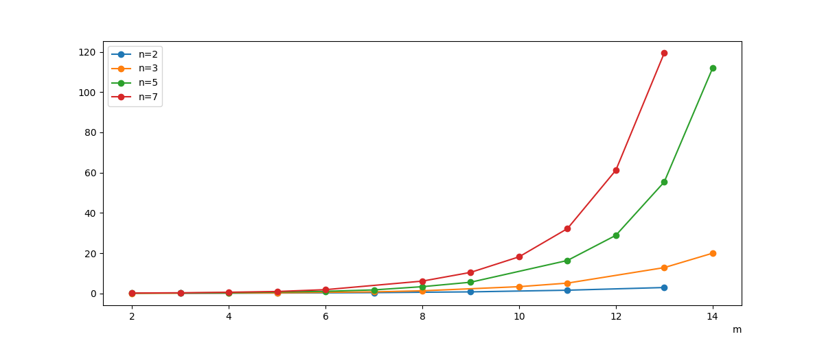
Figure 1: Time (in seconds) spent when calling the method almost_commuting_wilson for inputs $(n,m)$ ranging $n=2,3,5,7$ and $m=2,\ldots,14$. Each line represents the different times for a specific value of $n$ while values for $m\equiv 0\ (mod\ n)$ are skipped since they are not representative for time considerations.

It can be appreciated that the times are still reasonable (not bigger than 120 seconds). We would like to remark that the bigger result (in space) is the case with $n=7$ and $m=13$, where all data structures takes 4MB of disk space. Mathematically speaking, this result ($n=7$, $m=13$) contains the polynomial $P_{13}$ for $L_{7}$ with 830 monomials, and the 6 differential polynomials $H_{13,i}$ all with degree 7 and ranging from 744 up to 5279 monomials. The script that generates the figure (i.e., measures the times and generates the image) can be found in folder experiments in the aforementioned repository, in the file almost_commuting.sage.

6.2 Results available

In order to make the computed operators available to public usage, we have published a GitHub repository with several files with the results for $n=2,3,5,7$ and $m=2,\ldots,15$. The repository is called da_wilson and it is available in the following link.

https://github.com/Antonio-JP/da_wilson

In this repository we keep for each $n$ and $m$ stored a set of different files.

• An .out file containing the serialize version of the output of method almost_commuting_wilson. This contains both the polynomial $P_{m}$ and the list of $H_{m,i}$.

• A series of .tex files containing the LaTeX representation of the elements in the .out file. One file for the polynomial $P_{m}$ and one file for each of the differential polynomials $H_{m,i}$ for $i=0,\ldots,n-1$.

• A series of .mpl files containing a Maple representation of the elements in the .out file. Similar to the .tex files, we store the polynomial $P_{m}$ and the polynomials $H_{m,i}$ in separated files.

The names of the files follow this pattern: (n_m)[suf].ext, where;

• n and m will take the actual value of the data stored in the file,

• suf will indicate what element is in the file. P means the polynomial $P_{m}$ is in the file, while H_i indicates that the polynomial $H_{m,i}$ is stored in that file. For the .out files, this suffix will not appear.

• ext indicates the extension of the file, meaning the format in which the object is represented.

We refer to the README in this repository for explanation on advice on how to load data from these files into the different systems. Also, the script for generating all the Maple and TeX files is included in this repository.

Acknowledgements. The authors are partially supported by the grant PID2021-124473NB-I00, “Algorithmic Differential Algebra and Integrability” (ADAI) from the Spanish MICINN. The first author was partially supported by the Poul Due Jensen Grant 883901.

References

• [1] Bilge, A. H. A REDUCE program for the integration of differential polynomials. Computer Physics Communications 71, 3 (sep 1992), 263–268.
• [2] Boulier, F., Lemaire, F., Lallemand, J., Regensburger, G., and Rosenkranz, M. Additive normal forms and integration of differential fractions. Journal of Symbolic Computation 77 (nov 2016), 16–38.
• [3] Clarkson, P. Rational solutions of the classical Boussinesq system. Nonlinear Analysis: Real World Applications 10, 6 Spec (December 2009), 3360–3371. Conference on Differential Equations, Continuum Mechanics and Applications Univ Cape Town, Cape Town, South Africa, Oct 31st -Nov 2nd, 2007.
• [4] Davletshina, V. N., and Shamaev, E. On commuting differential operators of rank 2. Sib Math J 55, 4 (2014), 606–610.
• [5] Dickey, L. A. Soliton equations and Hamiltonian systems, vol. 26. World Scientific, 2003.
• [6] Drinfel’d, V. G., and Sokolov, V. V. Lie algebras and equations of korteweg-de vries type. Journal of Soviet Mathematics 30, 2 (July 1985), 1975–2036.
• [7] Goodearl, K. Centralizers in differential, pseudo-differential and fractional differential operator rings. Rocky Mountain J. Math. 13, 4 (1983), 573–618.
• [8] Grünbaum, F. A. Commuting pairs of linear ordinary differential operators of orders four and six. Phys. D 31 (1988), 424–433.
• [9] Jiménez-Pastor, A., Rueda, S. L., and Zurro, M.-A. Computing almost-commuting basis of ordinary differential operators. ACM Communications in Computer Algebra 57, 3 (Sept. 2023), 111–118.
• [10] Kolchin, E. R. Differential algebra and algebraic groups. No. 54 in Pure and Applied Mathematics. Academic Press, Boston, MA, 1973.
• [11] Krichever, I. M., and Novikov, S. P. Holomorphic bundles over algebraic curves and nonlinear equations. Russian Math. Surveys 35, 6 (1980), 53–79.
• [12] Mulase, M. Geometric classification of commutative algebras of ordinary differential operators. J. Diff. Geom. 19 (1990), 13–27.
• [13] Previato, E., , Rueda, S. L., Zurro, M.-A., and and. Commuting ordinary differential operators and the dixmier test. Symmetry, Integrability and Geometry: Methods and Applications (dec 2019).
• [14] Ritt, J. Differential algebra, vol. 33. American Mathematical Soc., 1950.
• [15] Rueda, S. L., and Zurro, M.-A. Factoring third order ordinary differential operators over spectral curves, 2021.
• [16] Rueda, S. L., and Zurro, M.-A. Spectral curves for third-order odos. Axioms 13, 4 (Apr. 2024), 274.
• [17] Schur, I. Über vertauschbare lineare Differentialausdrücke. Berlin Math. Gesellschaft, Sitzungsbericht. Arch. der Math., Beilage 3, 8 (1904), 2–8.
• [18] Segal, G., and Wilson, G. Loop groups and equations of KdV type. Publications mathématiques de l’IHÉS 61, 1 (Dec. 1985), 5–65.
• [19] The Sage Developers. SageMath, the Sage Mathematics Software System (Version 9.7), 2023. https://www.sagemath.org.
• [20] Wilson, G. Algebraic curves and soliton equations. In Geometry Today, E. A. et al., Ed. Birkhäuser, Boston, 1985, pp. 303–329.
• [21] Wilson, G. Algebraic curves and soliton equations. In Geometry Today (1985), E. A. et al., Ed., Birkhäuser, Boston, pp. 303–329.
• [22] Zheglov, A. Algebra, Geometry and Analysis of Commuting Ordinary Differential Operators. Moscow State University, Moscow, 2020.