Decompounding under general mixing distributions

Abstract.

This study focuses on statistical inference for compound models of the form $X=\xi_{1}+\ldots+\xi_{N}$, where $N$ is a random variable denoting the count of summands, which are independent and identically distributed (i.i.d.) random variables $\xi_{1},\xi_{2},\ldots$. The paper addresses the problem of reconstructing the distribution of $\xi$ from observed samples of $X$’s distribution, a process referred to as decompounding, with the assumption that $N$’s distribution is known. This work diverges from the conventional scope by not limiting $N$’s distribution to the Poisson type, thus embracing a broader context. We propose a nonparametric estimate for the density of $\xi,$ derive its rates of convergence and prove that these rates are minimax optimal for suitable classes of distributions for $\xi$ and $N$. Finally, we illustrate the numerical performance of the algorithm on simulated examples.

1. Introduction

Consider a random variable $X$ defined as a sum of a random number $N$ of independent and identically distributed (i.i.d.) random variables $\xi_{1},\xi_{2},\ldots$, i.e.,

$$X=\sum_{k=1}^{N}\xi_{k},$$

where $N$ and $\xi_{1},\xi_{2},\ldots$ are independent. This model can be seen as a generalization of Poisson random sums, which corresponds to the case when $N$ follows the Poisson distribution. Given a sample from this model, a natural question is how to estimate the distribution of $\xi_{1}$, assuming that the distribution of $N$ is known. This problem has been explored in several studies, primarily within a parametric framework and especially when $N$ is Poisson-distributed. A critical observation in nearly all these studies is that the characteristic function of $X$ equals the superposition of the probability generating function of $N$ and the characteristic function of $\xi$,

$$\phi_{X}(u)=\mathsf{E}[e^{\mathrm{i}uX}]=\mathcal{P}_{N}(\phi_{\xi}(u))\quad\text{with}\quad\mathcal{P}_{N}(z)=\sum_{k=1}^{\infty}\mathtt{p}_{k}z^{k},\quad\mathtt{p}_{k}={\mathsf{P}}(N=k),$$

where $\phi_{\xi}(u)=\mathsf{E}[e^{iu\xi}]$ is the characteristic function of $\xi$. Therefore, the function $\phi_{\xi}(u)$ (and hence the distribution of $\xi$) can be recovered if the inverse function of $\mathcal{P}_{N}$ is well-defined and precisely known. In simpler cases, such as when $N$ has a Poisson or geometric distribution, this process is straightforward. In the case when $\xi$ is a discrete random variable, one can use the recursion formulas (known as the Panjer recursions in the context of actuarial calculus, see Johnson et al., [12]) to recover the distribution of $\xi$. For other methods of this type, we refer to the monograph by Sundt and Vernic [13]. However, the problem is inherently ill-posed; minor perturbations in $\phi_{X}$ (e.g., due to limited data) can result in significant errors in $\phi_{\xi}(u)$. In addressing the statistical aspect of this problem, the concept of Panjer recursion was utilized by Buchmann and Grübel [4], [5], who are credited with introducing the term “decompounding”. Subsequently, other estimation methods were developed for the same model, including kernel-based estimates (Van Es et al.  [16]), convolution power estimates (Comte et al. [8]), spectral approach (Coca [7]) and Bayesian estimation techniques (Gugushvili et al. [10]). Let us stress that all these methods are designed for the case when $N$ has a Poisson distribution. The case of a generally distributed $N$ was examined by Bøgsted and Pitts [3], who proposed inverting $\mathcal{P}_{N}$ via series inversion. However, they did not provide convergence rates, and their approach requires that $\xi_{1}$ be positive with probability $1$ and $N$ take the value 1 with positive probability.

It’s worth noting that there’s a significant demand for broader classes for the distribution of $N$ across different applied disciplines, such as actuarial science and queuing theory. Asmussen and Albrecher [1] suggested that the widespread use of the Poisson distribution in actuarial models is largely attributed to its analytical simplicity and the ease with which its results can be interpreted, rather than any concrete evidence of its efficacy. Meanwhile, the exploration of non-Poisson arrival processes in queuing theory has been the focus of numerous studies. For instance, the work by Chydzinski  [6] delves into these processes, offering insights that can be contrasted with findings from Poisson-based models, as seen in the paper by Hansen and Pitts [11] or den Boer and Mandjes [9].

Contribution. This paper makes two significant contributions. Firstly, we conduct an in-depth theoretical analysis of the underlying statistical inverse problem when $N$, the count variable, has a general distribution. Our approach leverages the equation

(1.1) $$\phi_{X}(u)=\mathcal{L}_{N}\bigl{(}-\psi_{\xi}(u)\bigr{)}$$

where $\mathcal{L}_{N}(w)=\mathsf{E}[e^{-wN}]$ for $w\in\mathbb{C}$, is the Laplace transform of $N$, and $\psi_{\xi}(u)=\log(\phi_{\xi}(u))$, assuming the principal branch of the complex logarithm and that the characteristic function of $\xi$ is devoid of real zeros. The method involves estimating $\psi_{\xi}$ by inverting $\mathcal{L}_{N}(w)$ with respect to $w$. Following this, we apply the regularized inverse Fourier transform to approximate the density of $\xi$. Secondly, the paper establishes convergence rates for the proposed density estimate across various distribution classes, demonstrating that these rates achieve minimax optimality. Notably, we find that when $\mathsf{P}(N=1)>0$, the minimax convergence rates align with those obtained from direct observations of $X$. This marks the first instance of deriving minimax rates for general $N$ scenarios in existing literature.

Structure. The paper is organised as follows. In the next section we present the estimation procedure and show the rates of convergence to the true density. Subsection 2.1 is devoted to the nonasymptotic properties of the proposed estimate. The main result of this section, Theorem 2.1, gives the upper bound of the MSE on the sequence of events $\mathcal{A}_{n}$, the probabilities of which tend to 1 rather fast provided that some conditions are fulfilled (see corollaries 2.2 - 2.4 and examples in subsection 2.2). Next, in subsection 2.3, we show the asymptotic upper bounds for several classes of distributions (Theorem 2.8) and prove that these bounds are minimax optimal (Theorem 2.9). Section 3 contains several numerical examples showing the efficiency of the proposed algorithm and illustrating the difference between various classes of distributions. Finally, in section 4, we discuss the case ${\mathsf{P}}(N=1)=0$, which is significantly more difficult, as was mentioned also in previous papers on the topic (see, e.g., discussion in the paper by Bøgsted and Pitts [3]). The proofs are collected in section 5.

2. Main results

The key idea of the estimation procedure is to apply the inverse Laplace transform of $N$ (with respect to its complex-valued argument) to both parts of the equality (1.1), that is,

(2.1) $$\psi_{\xi}(u)=-\mathcal{L}^{-1}_{N}(\phi_{X}(u)),\quad u\in\mathbb{R}.$$

Note that $\mathcal{L}_{N}(w)$ is an analytic function for any $w$ with $\operatorname{Re}(w)>0$ (in particular, for $w=-\psi_{\xi}(u),\;u\in\mathbb{R}$), and therefore the inverse function $\mathcal{L}^{-1}_{N}$ exists and is analytic at the point $\phi_{X}(u)$, provided that

(2.2) $$(\mathcal{L}_{N})^{\prime}\left(-\psi_{\xi}(u)\right)\neq 0,\quad u\in\mathbb{R}.$$

Note that if ${\mathsf{E}}[N]<\infty,$ we have

$$(\mathcal{L}_{N})^{\prime}\left(-\psi_{\xi}(u)\right)=\sum\limits_{k=1}^{\infty}k(\phi_{\xi}(u))^{k}p_{k}={\mathsf{E}}[N]\phi_{\Lambda}(u),$$

where $\phi_{\Lambda}(u)$ is the characteristic function of the random variable $\Lambda=\xi_{1}+...+\xi_{\tau}$ with $\tau$ such that ${\mathsf{P}}(\tau=k)=k\mathtt{p}_{k}/{\mathsf{E}}[N],k=1,2,\dots$, and therefore (2.2) is equivalent to $\phi_{\Lambda}(u)\neq 0,\;u\in\mathbb{R}.$ This assumption holds under rather simple sufficient conditions (see Appendix B). We won’t be discussing these conditions here as we need to generalise (2.2) to determine the convergence rates in the next section. More precisely, we will assume that $(\mathcal{L}_{N})^{\prime}(z)\neq 0$ not only at the point $-\psi_{\xi}(u)$, but also in some vicinity of this point, which we will specify later.

The formula (2.1) suggests the following estimation scheme. First, we estimate the characteristic function $\phi_{\xi}(u)$ based on a sample $X_{1},\ldots,X_{n}$ from the distribution of $X$ using the empirical characteristic function $\widehat{\phi}_{X}(u)=n^{-1}\sum_{k=1}^{n}e^{\mathrm{i}uX_{k}}.$ Second, we estimate the function $\psi_{\xi}$ via $\widehat{\psi}_{\xi}(u)=-\mathcal{L}^{-1}_{N}(\widehat{\phi}_{X}(u))$ and get estimate for the characteristic function of $\phi_{\xi}$ as $\widehat{\phi}_{\xi}(u)=\exp(\widehat{\psi}_{\xi}(u)).$ Note that $\mathcal{L}^{-1}_{N}(\widehat{\phi}_{X}(u))$ is well defined for $u$ in some vicinity of $0$ due to $\operatorname{Re}[\widehat{\phi}_{\xi}(0)]=1.$ Finally, we use a regularised inverse Fourier transform to estimate the distribution of $\xi.$ So, the scheme is as follows:

$$\boxed{X_{1},\dots,X_{n}\;\rightarrow\;\widehat{\phi}_{X}(u)\;\rightarrow\;\widehat{\psi}_{\xi}(u)\;\rightarrow\;\widehat{\phi}_{\xi}(u)\rightarrow\;\text{Law}(\xi).}$$

Assuming that the distribution of $\xi$ is absolutely continuous with density $p_{\xi}$, the estimation scheme explained above leads to the following estimator

(2.3) $$\widehat{p}_{\xi}(x):=\frac{1}{2\pi}\int_{-U_{n}}^{U_{n}}e^{-\mathrm{i}ux}\widehat{\phi}_{\xi}(u)\,du=\frac{1}{2\pi}\int_{-U_{n}}^{U_{n}}\exp\left\{-\mathrm{i}ux-\mathcal{L}^{-1}_{N}\bigl{(}\widehat{\phi}_{X}(u)\bigr{)}\right\}\,du$$

for any $x\in\mathbb{R},$ where $U_{n}$ is a sequence of positive numbers tending to infinity at a proper rate in order to ensure that $\mathcal{L}^{-1}_{N}\bigl{(}\widehat{\phi}_{X}(u)\bigr{)}$ for $u\in[-U_{n},U_{n}]$ is well defined on an event of positive probability.

2.1. Nonasymptotic bounds

Introduce the function

$$\mathcal{H}(z):=\exp(-\mathcal{L}^{-1}_{N}(z)),\qquad z\in\mathcal{C},$$

where $\mathcal{C}$ is the region of analyticity of the function $\mathcal{H}.$ The discussion above imples that $\phi_{X}(u)\in\mathcal{C}\;\;\forall u\in\mathbb{R},$ provided that $\phi_{\Lambda}$ doesn’t vanish on $\mathbb{R}$. The first derivative of this function is equal to

(2.4) $$\mathcal{H}^{\prime}(z)=-\frac{\exp(-\mathcal{L}^{-1}_{N}(z))}{\left(\mathcal{L}_{N}\right)^{\prime}\left(\mathcal{L}^{-1}_{N}(z)\right)}=-\frac{1}{\sum_{k=1}^{\infty}k\texttt{p}_{k}e^{-(k-1)\mathcal{L}^{-1}_{N}(z)}},\qquad z\in\mathcal{C},$$

while the direct calculation of the second derivative yields

(2.5) $$\mathcal{H}^{\prime\prime}(z) = (\mathcal{H}^{\prime}(z))^{3}\sum_{k=2}^{\infty}\mathtt{p}_{k}(k^{2}-k)\exp(-(k-2)\mathcal{L}^{-1}_{N}(z)),\qquad z\in\mathcal{C}.$$

At the point $z=\phi_{X}(u),u\in\mathbb{R}$, these derivatives are equal to

$$\mathcal{H}^{\prime}\bigl{(}\phi_{X}(u)\bigr{)} = -\frac{\phi_{\xi}(u)}{(\mathcal{L}_{N})^{\prime}(-\psi_{\xi}(u))}=-({\mathsf{E}}[N])^{-1}\frac{\phi_{\xi}(u)}{\phi_{\Lambda}(u)},$$

$$\mathcal{H}^{\prime\prime}\bigl{(}\phi_{X}(u)\bigr{)} = (\mathcal{H}^{\prime}(\phi_{X}(u)))^{3}\sum_{k=2}^{\infty}\mathtt{p}_{k}(k^{2}-k)\bigl{(}\phi_{\xi}(u)\bigr{)}^{k},$$

and therefore are uniformly bounded on $\mathbb{R}$, provided that ${\mathsf{E}}[N^{2}]<\infty,\mathtt{p}_{1}>0$ and (2.2) holds. Indeed, $\phi_{\Lambda}$ doesn’t vanish on $\mathbb{R}$, and in this case $\mathcal{H}^{\prime}\bigl{(}\phi_{X}(u)\bigr{)}$ is bounded as a continuous function since its limit for $u\to\infty$ equals to $-({\mathsf{E}}[N]\mathtt{p}_{1})^{-1}$ . Moreover, $\mathcal{H}^{\prime\prime}\bigl{(}\phi_{X}(u)\bigr{)}$ is bounded due to the trivial estimate $|\mathcal{H}^{\prime\prime}\bigl{(}\phi_{X}(u)\bigr{)}|\leq|\mathcal{H}^{\prime}\bigl{(}\phi_{X}(u)\bigr{)}|^{3}({\mathsf{E}}[N^{2}]+{\mathsf{E}}[N]),u\in\mathbb{R}.$

In what follows, we need a boundedness of $\mathcal{H}^{\prime}(z)$ and $\mathcal{H}^{\prime\prime}(z)$ in some vicinity of the point $z=\phi_{X}(u)$. More precisely, we introduce the following event

$$\mathcal{A}_{n}(\varkappa):=\biggl{\{}\phi_{X,\tau}(u)\in\mathcal{C},\;\forall\tau\in[0,1],\;\forall u\in[-U_{n},U_{n}]\biggr{\}}\\ \cap\biggl{\{}\max_{\tau\in[0,1]}\max\limits_{|u|\leq U_{n}}\max\bigl{\{}|\mathcal{H}^{\prime}\bigl{(}\phi_{X,\tau}(u)\bigr{)}|,|\mathcal{H}^{\prime\prime}\bigl{(}\phi_{X,\tau}(u)\bigr{)}|\bigr{\}}\leq\varkappa\biggr{\}},$$

where $\phi_{X,\tau}(u):=\phi_{X}(u)+\tau(\widehat{\phi}_{X}(u)-\phi_{X}(u))$ and $\varkappa>0.$ Note that if this event has positive probability for all $n$, then the assumption (2.2) holds.

Now let us formulate the main result of this section.

Theorem 2.1.

Suppose that $\phi_{\xi}\in L_{1}(\mathbb{R})$ with $C_{\phi}:=\|\phi_{\xi}\|_{L^{1}(\mathbb{R})}.$ Let us fix some $\varkappa>0$ such that $q_{n}=q_{n}(\varkappa):={\mathsf{P}}(\mathcal{A}_{n}(\varkappa))>0$ for all $n>n_{0}.$ Assume also that ${\mathsf{E}}[N^{2}]<\infty$, then it holds

(2.6) $${\mathsf{E}}\left[\left|\widehat{p}_{\xi}(x)-p_{\xi}(x)\right|^{2}\Bigr{|}\mathcal{A}_{n}\right]\lesssim\biggl{(}\int_{|u|>U_{n}}\left|\phi_{\xi}(u)\right|\,du\biggr{)}^{2}+\varkappa^{2}\frac{U_{n}}{n\,q_{n}}C_{\phi}{\mathsf{E}}[N]+\varkappa^{2}\frac{U_{n}^{2}}{n^{2}q_{n}^{2}}\\ +\varkappa^{2}\frac{U_{n}^{2}}{n\,q_{n}}(1-q_{n})^{1/2}+\varkappa\frac{U_{n}^{2}}{n^{3/2}\,q_{n}^{1/2}},\qquad n>n_{0},$$

where $\lesssim$ stands for inequality up to an absolute constant not depending on $n$ and distributions of $\xi,N.$

Let us next mention several rather general situations where the probability of the event $\mathcal{A}_{n}$ can be estimated from below.

Corollary 2.2.

Suppose that the distribution of $\xi$ is symmetric, then by changing the empirical cf $\widehat{\phi}_{X}(u)$ to its real part we have that $\phi_{X,\tau}(u)\in[-1,1]$ for all $u\in\mathbb{R}.$ Hence, with probability $1,$

$$|\mathcal{H}^{\prime}(\phi_{X,\tau}(u))|=\left[\sum_{k=1}^{\infty}k\,\mathtt{p}_{k}\exp\bigl{(}-(k-1)\mathcal{L}^{-1}_{N}(\phi_{X,\tau}(u))\bigr{)}\right]^{-1}\leq\frac{1}{\mathtt{p}_{1}},\quad\tau\in[0,1],\quad u\in\mathbb{R},$$

provided $\mathtt{p}_{1}>0.$ Furthermore, we have that $\mathcal{L}^{-1}_{N}(\phi_{X,\tau}(u))\geq 0$ for all $u\in\mathbb{R}$ and $\tau\in[0,1]$ with probability $1$ due to the fact that

$$\mathcal{L}_{N}(z)=\sum_{k=1}^{\infty}\mathtt{p}_{k}e^{-zk}\in[0,1]\quad\text{iff}\quad z\geq 0.$$

Therefore, from (2.5) we get

$$|\mathcal{H}^{\prime\prime}(\phi_{X,\tau}(u))| \leq \frac{{\mathsf{E}}[N^{2}]-{\mathsf{E}}[N]}{\mathtt{p}_{1}^{3}}=:\varkappa,$$

and conclude that under this choice of $\varkappa$, we have $q_{n}={\mathsf{P}}(\mathcal{A}_{n}(\varkappa))=1$ for all $n\geq 1.$

Corollary 2.3.

Suppose that there is $\rho_{0}>1$ such that

(2.7) $$|\mathcal{H}^{\prime}(z)|\leq\varkappa,\quad|\mathcal{H}^{\prime\prime}(z)|\leq\varkappa,\qquad\forall\;z\in\mathbb{C}:|z|\leq\rho_{0}$$

for some finite $\varkappa=\varkappa(\rho_{0}).$ In this case, we obviously have ${\mathsf{P}}(\mathcal{A}_{n}(\varkappa))=1$ since $|\phi_{X,\tau}(u)|\leq 1$ for all $u$ and $\tau.$

Corollary 2.4.

Assume that $\operatorname{Re}(\phi_{X}(u))\neq 0\;\;\forall u\in\mathbb{R},$  and

(2.8) $$|\mathcal{H}^{\prime}(z)|\leq\varkappa,\quad|\mathcal{H}^{\prime\prime}(z)|\leq\varkappa,\qquad\forall\;z\in\mathbb{C}:\operatorname{Re}(z)>-\rho_{1}$$

for some $\rho_{1}>0$ and some finite $\varkappa=\varkappa(\rho_{1}).$ Then using the fact that $\operatorname{Re}(\phi_{X}(u))\geq 0$ for all $u\in\mathbb{R}$ and Proposition 3.3 from [2], we derive

$$1-q_{n}={\mathsf{P}}(\mathcal{A}_{n}^{c}) \leq {\mathsf{P}}(\exists\tau\in[0,1],\exists u\in[-U_{n},U_{n}]:\operatorname{Re}(\phi_{X,\tau}(u))\leq-\rho_{1})$$

$$\leq {\mathsf{P}}\bigl{(}\|\phi_{X}-\widehat{\phi}_{X}\|_{[-U_{n},U_{n}]}\geq\rho_{1}\bigr{)}\lesssim\left(\sqrt{n}U_{n}\right)^{-2},$$

provided that $18\sqrt{\log(nU_{n}^{2})/n}<\rho_{1}.$

2.2. Examples

In this section we discuss several important examples including two-point distribution and Poisson like distribution for $N.$

Example 2.5.

Let $N$ take two values, 1 and 2, with probabilities $p\in(0,1)$ and $1-p$, respectively. Then

(2.9) $$\mathcal{L}_{N}(z)=pe^{-z}+(1-p)e^{-2z},\quad\forall z\in\mathbb{C}.$$

The inversion of the Laplace transform (2.9) leads to

$$\mathcal{L}_{N}^{-1}(z) = -\log\Bigl{(}\frac{-p+\sqrt{p^{2}+4z(1-p)}}{2(1-p)}\Bigr{)},$$

and therefore the function $\mathcal{H}$ and its first and second derivatives are equal to

$$\mathcal{H}(z) = \frac{-p+\sqrt{p^{2}+4z(1-p)}}{2(1-p)},$$

$$\mathcal{H}^{\prime}(z) = \frac{1}{\sqrt{p^{2}+4z(1-p)}},$$

$$\mathcal{H}^{\prime\prime}(z) = -\frac{2(1-p)}{\bigl{(}p^{2}+4z(1-p)\bigr{)}^{3/2}}.$$

If $\rho^{*}:=p^{2}/(4(1-p))>1$ the condition (2.7) holds with $1<\rho_{0}<\rho^{*}$ and

(2.10) $$\varkappa=\varkappa(\rho_{0}):=\max\Bigl{\{}\mathcal{H}^{\prime}(-\rho_{0}),-\mathcal{H}^{\prime\prime}(-\rho_{0})\Bigr{\}}.$$

On the other hand, the condition (2.8) is also fulfilled for $0<\rho_{1}<\rho^{*}$ and $\varkappa=\varkappa(\rho_{1})$. As compared to (2.7), we do need to assume that $\rho^{*}>1,$ but have to check the condition  $\operatorname{Re}(\phi_{X}(u))\neq 0\;\;\forall u\in\mathbb{R},$ which depends on the distribution of $\xi$.

Example 2.6.

Let $N$ be distributed according to the shifted Poisson law, that is,

$${\mathsf{P}}(N=k)=\mathtt{c}_{\lambda}\frac{\lambda^{k}}{k!},\quad k=1,2,\dots,$$

where $\lambda>0$ and $\mathtt{c}_{\lambda}:=1/(e^{\lambda}-1)$. In this case,

$$\mathcal{L}_{N}(z)=\mathtt{c}_{\lambda}\bigl{(}e^{\lambda e^{-z}}-1\bigr{)},\qquad\mathcal{L}^{-1}_{N}(z)=-\log\Bigl{(}\frac{1}{\lambda}\log\left(z/\mathtt{c}_{\lambda}+1\right)\Bigr{)},$$

where the formula for the inverse function is valid for for all $z\in\mathbb{C}\setminus\mathbb{R}_{\leq 0}$. Consequently direct calculations yield

$$\mathcal{H}(z) = \frac{1}{\lambda}\log\left(z/\mathtt{c}_{\lambda}+1\right),$$

$$\mathcal{H}^{\prime}(z) = \frac{1}{\lambda\bigl{(}\mathtt{c}_{\lambda}+z\bigr{)}},$$

$$\mathcal{H}^{\prime\prime}(z) = -\frac{1}{\lambda\bigl{(}\mathtt{c}_{\lambda}+z\bigr{)}^{2}}.$$

Again the condition (2.7) holds with $1<\rho_{0}<\mathtt{c}_{\lambda}$ and$\varkappa=\varkappa(\rho_{0})$ given by (2.10) with $\mathcal{H}^{\prime},\mathcal{H}^{\prime\prime}$ as above, provided $\mathtt{c}_{\lambda}>1.$ Similarly, the condition (2.8) is also fulfilled for $0<\rho_{1}<\mathtt{c}_{\lambda}$ and $\varkappa=\varkappa(\rho_{1}).$

Example 2.7.

Let $N$ be geometrically distributed with parameter $p\in(0,1)$, that is,

$${\mathsf{P}}(N=k)=(1-p)^{k-1}p,\quad k=1,2,\ldots.$$

In this case, one observes that

$$\mathcal{L}_{N}(z) = \frac{pe^{-z}}{1-(1-p)e^{-z}},\quad\operatorname{Re}(z)>\log(1-p),$$

$$\mathcal{L}^{-1}_{N}(z) = -\log\left(\frac{z}{p+z(1-p)}\right),\quad z\neq-p/(1-p).$$

Direct calculations lead to the following formulas for any $z\neq-p/(1-p):$

$$\mathcal{H}(z) = \frac{z}{p+z(1-p)},$$

$$\mathcal{H}^{\prime}(z) = \frac{p}{(p+z(1-p))^{2}},$$

$$\mathcal{H}^{\prime\prime}(z) = \frac{-2p(1-p)}{(p+z(1-p))^{3}},$$

and we conclude that if $\rho^{\star}:=p/(1-p)>1$ (that is, $p>1/2$) the condition (2.7) holds with $1<\rho_{0}<\rho^{\star}$ and $\varkappa=\varkappa(\rho_{0}).$ On the other hand, the condition (2.8) is also fulfilled for $0<\rho_{1}<\rho^{\star}$ and $\varkappa=\varkappa(\rho_{1}).$ Compared to (2.7), here we do need to assume that $\rho^{\star}>1.$

2.3. Minimax rates of convergence

Fix some $\beta,\gamma>0,$ $M>0$ and consider two classes of probability densities functions

$$\mathcal{C}(\beta,M):=\biggl{\{}p\in\mathcal{L}_{1}(\mathbb{R}),\,p\geq 0:\quad\sup_{u\in\mathbb{R}}\Bigl{\{}(1+|u|)^{1+\beta}|\phi_{p}(u)|\Bigr{\}}\leq M\biggr{\}}$$

and

$$\mathcal{E}(\gamma,M):=\biggl{\{}p\in\mathcal{L}_{1}(\mathbb{R}),\,p\geq 0:\quad\sup_{u\in\mathbb{R}}\Bigl{\{}\exp(c_{\gamma}|u|^{\gamma})|\phi_{p}(u)|\Bigr{\}}\leq M\biggr{\}},$$

where

$$\phi_{p}(u)=\int_{\mathbb{R}}e^{\mathrm{i}ux}p(x)\,dx,\qquad u\in\mathbb{R},$$

is the characteristic function of the random variable with the density $p$.

Theorem 2.8.

Suppose that for some $\varkappa>1$, it holds $U_{n}\sqrt{1-q_{n}(\varkappa)}\leq 1$ for all $n>n_{0},$ that is, ${\mathsf{P}}(\mathcal{A}_{n})\geq 1-U_{n}^{-2}.$

(i) If $p_{\xi}\in\mathcal{C}(\beta,M)$ for some $\beta>1/2,M>0$ then

$$\max_{x\in\mathbb{R}}{\mathsf{E}}\left[\left|\widehat{p}_{\xi}(x)-p_{\xi}(x)\right|^{2}\Bigr{|}\mathcal{A}_{n}\right]\lesssim M^{2}U_{n}^{-2\beta}+C(M,\varkappa,N)\frac{U_{n}}{n}+\varkappa^{2}\frac{U_{n}^{2}}{n^{2}q_{n}^{2}},\quad n>n_{0},$$

where $C(M,\varkappa,N)=2\varkappa^{2}M\bigl{(}1+\beta^{-1}\bigr{)}{\mathsf{E}}[N].$ Furthermore, under the choice $U_{n}=n^{1/(1+2\beta)}$ we get

$$\max_{x\in\mathbb{R}}{\mathsf{E}}\left[\left|\widehat{p}_{\xi}(x)-p_{\xi}(x)\right|^{2}\Bigr{|}\mathcal{A}_{n}\right]\lesssim\max(M^{2},C(M,\varkappa,N))\,n^{-2\beta/(1+2\beta)},\quad n>n_{0}.$$

(ii) If $p_{\xi}\in\mathcal{E}(\gamma,M)$ for some $\gamma>\gamma_{\circ}$ with $\gamma_{\circ}>0$, and some $\gamma,M>0$ then

$$\max_{x\in\mathbb{R}}{\mathsf{E}}\left[\left|\widehat{p}_{\xi}(x)-p_{\xi}(x)\right|^{2}\Bigr{|}\mathcal{A}_{n}\right]\lesssim M^{2}U_{n}^{2(1-\gamma)}e^{-2c_{\gamma}U_{n}^{\gamma}}+\frac{U_{n}}{n}C(M,\varkappa,N)+\varkappa^{2}\frac{U_{n}^{2}}{n^{2}q_{n}^{2}},\\ \quad n>n_{0},$$

where $C(M,\varkappa,N)=2\varkappa^{2}M{\mathsf{E}}[N]\max\bigl{(}1,\Gamma(\gamma^{-1}_{\circ}+1)\bigr{)}c_{\gamma}^{-1/\gamma}.$ Under the choice

$$U_{n}=(\log n/(2c_{\gamma}))^{1/\gamma}$$

we get

$$\max_{x\in\mathbb{R}}{\mathsf{E}}\left[\left|\widehat{p}_{\xi}(x)-p_{\xi}(x)\right|^{2}\Bigr{|}\mathcal{A}_{n}\right]\lesssim\max(M^{2},C(M,\varkappa,N))\,\frac{(\log n)^{\max(1,2(1-\gamma))/\gamma}}{n},\\ n>n_{0}.$$

It follows from Corollary 2.2 that

$$\sup_{p_{\xi}\in\mathcal{C}(\alpha,M)}\max_{x\in\mathbb{R}}{\mathsf{E}}\left[\left|\widehat{p}_{\xi}(x)-p_{\xi}(x)\right|^{2}\right]\lesssim\max(M^{2},C(M,\varkappa,N))\,n^{-2\beta/(1+2\beta)},\quad n>n_{0},$$

provided that the distribution of $\xi$ is symmetric and $\mathtt{p}_{1}>0.$ As shown in the next theorem, these rates turn out to be minimax optimal.

Theorem 2.9 (Lower bounds).

Let ${\mathsf{P}}(N=1)>0$ and let $\mathrm{Sym}(\mathbb{R})$ be a class of symmetric functions on $\mathbb{R}$. Then it holds

$$\inf_{\widehat{p}}\sup_{p_{\xi}\in\mathcal{C}(\beta,M)\cap\mathrm{Sym}(\mathbb{R})}\max_{x\in\mathbb{R}}{\mathsf{E}}\left[\left|\widehat{p}_{\xi}(x)-p_{\xi}(x)\right|^{2}\right]\gtrsim n^{-2\beta/(1+2\beta)},$$

where infimum is taken over all estimates, that is, measurable functions of $X_{1},\ldots,X_{n}.$

3. Numerical examples

In the present section, we illustrate the proposed estimation procedure by a simulation study. Let us consider the following three cases of the law of $N$: the one supported on two points (see Example 2.5), the geometric distribution starting from 1 (see Example 2.7) or the shifted Poisson (as in Example 2.6). As for $\xi$, in what follows we consider the case when $\xi$ has either the Laplace distribution with zero mean and scale equal to one, or the standard normal distribution. It can be observed that in all these cases the c.f. $\phi_{X}(u)$ has the same behaviour as $\phi_{\xi}(u)$ as $|u|\to\infty$. Since in case when $\xi_{1}$ follows the Laplace distribution $\phi_{\xi}(u)=(1+u^{2})^{-1}$, it can be seen that for any $U_{n}>0$ the characteristic function $\phi_{X}(u)$ satisfies the condition of Theorem 2.8 with $\beta=1$, while in case of the normal law, as $\phi_{\xi}(u)=e^{-u^{2}/2}$, we get that $\phi_{X}(u)$ satisfies the condition of with $\alpha=1/2$ and $\gamma=2$.

For the simulation study, we fix the parameter of the law of $N$ as $p=0.3$ in case of the two-point and geometric distribution and $\lambda=1$ in case of the Poisson law. For all the considered cases — three with respect to the distribution of $N$ and two with respect to the law of $\xi_{1}$ — we aim at analysing the behaviour of the proposed estimator for different values of $n\in\{100,1000,5000\}$. To this end, we simulate 100 samples for every $n$ and compute the error

(3.1) $$\frac{1}{J}\sum\limits_{j=1}^{J}\left(\widehat{p}(x_{j})-p(x_{j})\right)^{2},$$

where $\{x_{j}\}_{1\leq j\leq J}$ is an equidistant grid of $J=1000$ points from $-4$ to $4$, $\widehat{p}$ is the proposed estimator (2.3), and $p$ is the density of either the Laplace or the standard normal distribution. As suggested by Theorem 2.8, in case when $\xi_{1}$ is normally distributed the truncating sequence is chosen as

$$U_{n}=((\log n)/(2c_{\gamma}))^{1/\gamma}.$$

As for the case of the Laplace distribution, Theorem 2.8 suggests that $U_{n}$ should be of order $n^{1/(2\alpha-1)}=n^{1/3}$. To speed up the numerical computations and ensure convergence of the integrals on finite data samples, we multiply this value by a normalising constant $c=1/3$, taking $U_{n}=cn^{1/3}$.

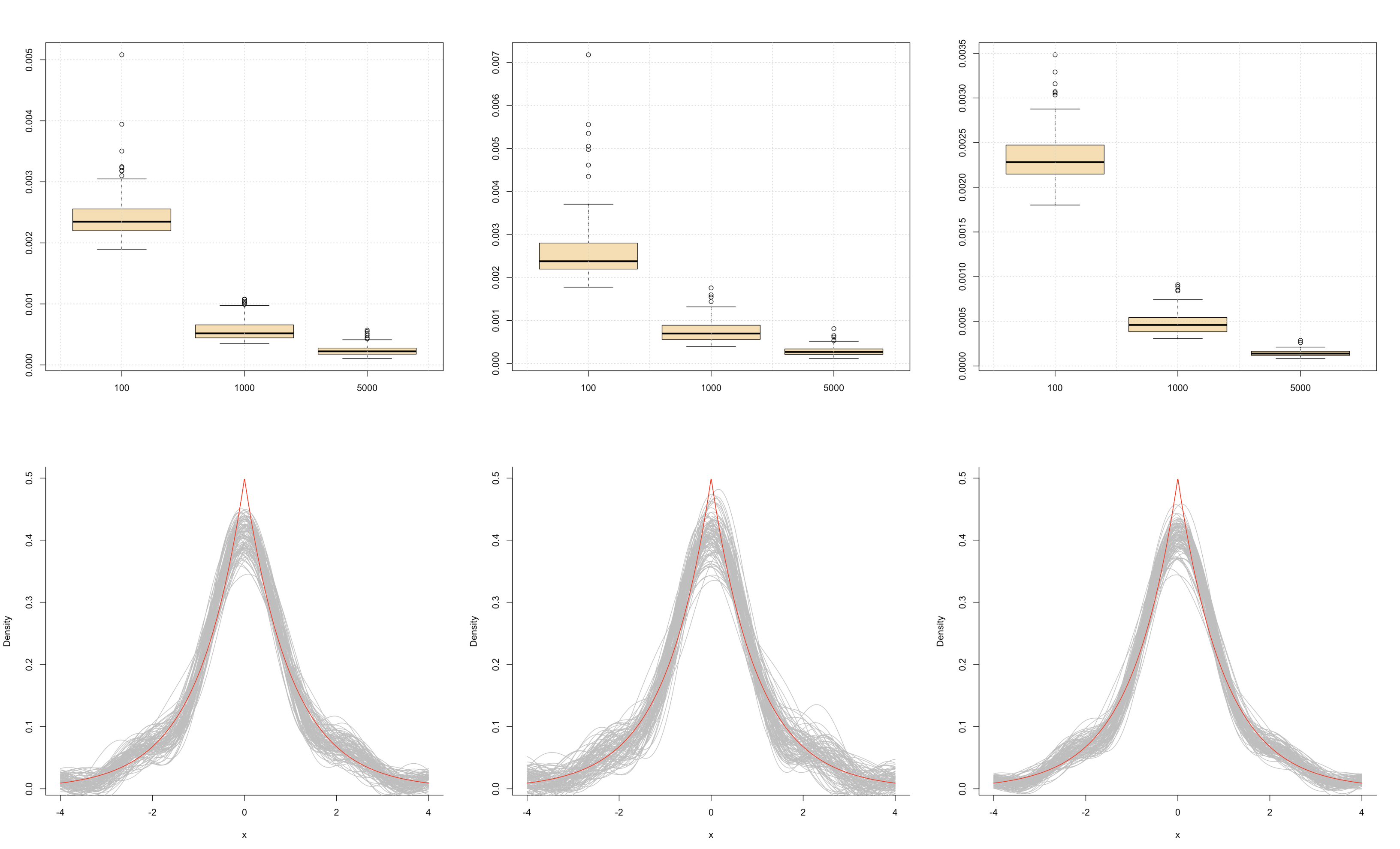
Figure 1. The errors (3.1) of the estimator (2.3) (top) and estimated and real densities of $\xi$ (bottom) for $N$ having the two point (left), geometric (middle) and shifted Poisson (right) distributions, and $\xi$ following the Laplace distribution.

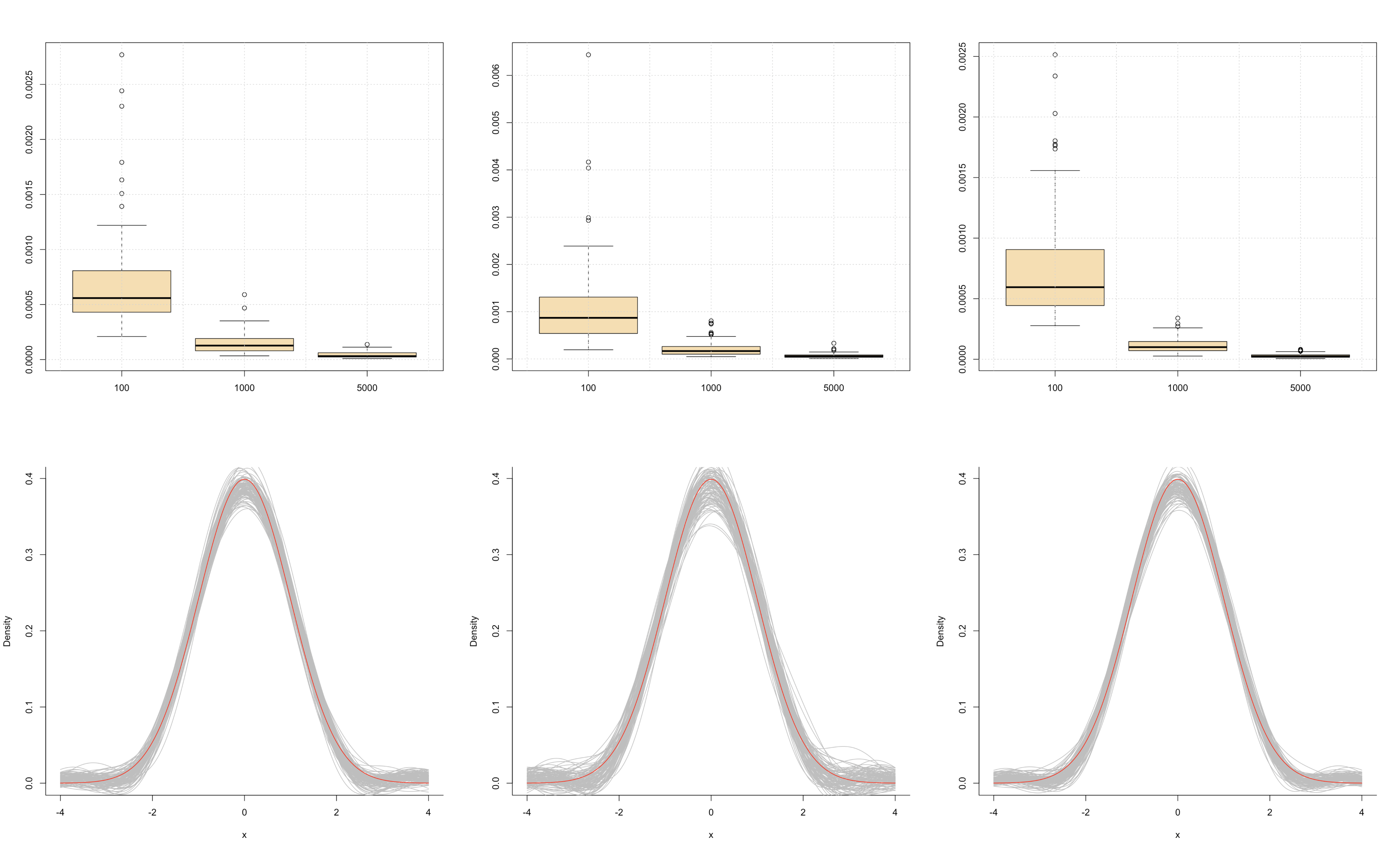
Figure 2. The errors (3.1) of the estimator (2.3) (top) and estimated and real densities of $\xi$ (bottom) for $N$ having the two point (left), geometric (middle) and shifted Poisson (right) distributions, and $\xi$ following the standard normal law.

The first row of Figures 1 and 2 represents the boxplots of errors (3.1) for the cases of Laplace and normal $\xi$, respectively, with different distributions of $N$ and sample sizes $n$. It can be observed that in all the considered cases the values of errors decline with the growth of sample size and are reasonably small, not exceeding 0.008 even for $n=100$. Also, it can be seen that the case when $\xi$ follows the normal distribution generally leads to smaller errors than the Laplace one. This observation is further supported by the second row of Figures 1 and 2, which depicts the true and estimated densities of $\xi$, as the estimates for the normal law appear to be much more stable than those for the Laplace distribution. It is worth mentioning that these results are fully coherent with our theoretical findings, yielding the faster rate of convergence in the case of the class $\mathcal{E}(\gamma,M)$. All in all, we conclude that the proposed estimation method allows to obtain favourable results for the considered examples, and hence can successfully be employed for the problems of this kind.

4. Discussion and extensions

Let’s delve into some discussions and extensions. A key point to consider is that when ${\mathsf{P}}(N=1)=0$, the complexity of the problem increases significantly. This particular scenario encompasses the challenging task of inferring the distribution of a random variable $\xi$ from the distribution of its sum $\xi_{1}+\xi_{2}+\ldots+\xi_{m}$ for a specified $m\in\mathbb{N}$. This task essentially boils down to the intricate process of reconstructing the characteristic function $\phi_{\xi}$ from its powers, which is recognized as an inherently difficult problem due to its ill-posed nature. An illustrative example can demonstrate this complexity: it has been established that there exists a distribution function $F$ such that the distribution of the sum of any number of independent random variables adhering to the law $F$ does not uniquely determine $F$. To elucidate this point, one might consider a distribution $F$ defined by the density function:

$$F^{\prime}(x)=p(x)=\frac{1-\cos(x)}{\pi x^{2}}(1-\cos(2x)),\qquad x\in\mathbb{R}.$$

Then by defining for any $m,$

$$G^{\prime}_{m}(x)=\frac{1-\cos(x)}{\pi x^{2}}\left(1-\cos\left(2x+\frac{2\pi}{m}\right)\right)$$

it easy to show that

$$\underbrace{F\star\ldots\star F}_{m}=\underbrace{G_{m}\star\ldots\star G_{m}}_{m}.$$

This example underscores the nuanced challenges encountered in this problem, highlighting the need for careful consideration and more restrictive assumptions. In this respect, the following result can be proved. Let us assume that the characteristic function $\phi_{\xi}$ doesn’t vanish on $\mathbb{R}$, and therefore $(\phi_{X})^{1/m}$ is well defined. Then an estimate of $p_{\xi}$ can be defined as

$$\widehat{p}_{\xi}(x)=\frac{1}{2\pi}\int_{-U_{n}}^{U_{n}}e^{-\mathrm{i}\omega x}(\widehat{\phi}_{X}(\omega))^{1/m}\,d\omega.$$

Since $(\widehat{\phi}_{X})^{1/m}$ is well defined only on the interval where $\widehat{\phi}_{X}\neq 0$ we will consider the event

$$\mathcal{B}_{n}(\varkappa):=\left\{\sup_{\omega\in[-U_{n},U_{n}]}\left|\frac{\widehat{\phi}_{X}(\omega)-\phi_{X}(\omega)}{\phi_{X}(\omega)}\right|\leq\varkappa\right\}$$

for some $\varkappa>0$. The following result holds.

Theorem 4.1.

Suppose that

$$M^{-1}\leq(1+|u|)^{\alpha}|\phi_{\xi}(u)|\leq M$$

for some $\alpha>1$ and $M>0.$ Assume that $\inf_{n>n_{0}}{\mathsf{P}}(\mathcal{B}_{n}(\varkappa))>0$ for some $\varkappa>0$. Then it holds for any $x\in\mathbb{R},$

(4.1) $${\mathsf{E}}\left[\left|\widehat{p}_{\xi}(x)-p_{\xi}(x)\right|^{2}\Bigr{|}\mathcal{B}_{n}\right]\lesssim U_{n}^{2(1-\alpha)}+\frac{U_{n}^{1+\alpha(2m-1)}}{n}$$

provided $U_{n}^{\alpha m}\,n^{-1/2}=o(1),$ $n\to\infty.$ Here $\lesssim$ stands for inequality up to an absolute constant not depending on $n.$

Corollary 4.2.

By choosing $U_{n}=n^{1/(\alpha-1+2m\alpha)},$ we derive

$${\mathsf{E}}\left[\left|\widehat{p}_{\xi}(x)-p_{\xi}(x)\right|^{2}\Bigr{|}\mathcal{B}_{n}\right]\lesssim n^{-2(\alpha-1)/(\alpha-1+2m\alpha)},$$

where ${\mathsf{P}}(\mathcal{B}_{n}^{c})\leq\left(\sqrt{n}U_{n}\right)^{-2}$.

5. Proofs

5.1. Proof of Theorem 2.1

It holds for all $x\in\mathbb{R}$,

$${\mathsf{E}}\left[\widehat{p}_{\xi}(x)|\mathcal{A}_{n}\right]-p_{\xi}(x)=\frac{1}{2\pi}\int_{|u|\leq U_{n}}e^{-\mathrm{i}ux}\,{\mathsf{E}}\left[e^{-\mathcal{L}^{-1}_{N}\left(\widehat{\phi}_{X}(u)\right)}-e^{-\mathcal{L}^{-1}_{N}\left(\phi_{X}(u)\right)}\big{|}\mathcal{A}_{n}\right]\,du\\ -\frac{1}{2\pi}\int_{|u|>U_{n}}e^{-\mathrm{i}ux+\psi_{\xi}(u)}\,du=I_{1}+I_{2}.$$

Applying Lemma A.1 to $\mathcal{H}(z)=\exp(-\mathcal{L}^{-1}_{N}(z))$ with $k=2$, $z=\widehat{\phi}_{X}(u)$, $a=\phi_{X}(u)$, we get

$${\mathsf{E}}\Bigl{[}e^{-\mathcal{L}^{-1}_{N}(\widehat{\phi}_{X}(u))}-e^{-\mathcal{L}^{-1}_{N}(\phi_{X}(u))}|\mathcal{A}_{n}\Bigr{]}={\mathsf{E}}\Bigl{[}{\mathsf{E}}_{\tau}[g_{\tau}(\widehat{\phi}_{X}(u),\phi_{X}(u))](\widehat{\phi}_{X}(u)-\phi_{X}(u))^{2}\Big{|}\mathcal{A}_{n}\Bigr{]}$$

where

$$g_{\tau}(\widehat{\phi}_{X}(u),\phi_{X}(u)):=(1-\tau)\mathcal{H}^{\prime\prime}\bigl{(}\phi_{X,\tau}(u)\bigr{)},\quad\phi_{X,\tau}(u):=\phi_{X}(u)+\tau(\widehat{\phi}_{X}(u)-\phi_{X}(u)).$$

On the event $\mathcal{A}_{n}$, we have $|\mathcal{H}^{\prime\prime}(\phi_{X,\tau}(u))|\leq\varkappa$ for all $\tau\in[0,1]$ and $|u|\leq U_{n}$, and hence

$$|I_{1}| \leq \frac{\varkappa}{2\pi}\int_{|u|\leq U_{n}}{\mathsf{E}}[(\widehat{\phi}_{X}(u)-\phi_{X}(u))^{2}|\mathcal{A}_{n}]\,du$$

$$\lesssim \frac{\varkappa}{{\mathsf{P}}(\mathcal{A}_{n})}\int_{|u|\leq U_{n}}\frac{1-|\phi_{X}(u)|^{2}}{n}\,du\lesssim\frac{\varkappa U_{n}}{nq_{n}}.$$

Furthermore

$$\operatorname{Var}\left(\widehat{p}(x)|\mathcal{A}_{n}\right) = \operatorname{Var}\left(\int_{-U_{n}}^{U_{n}}e^{-\mathrm{i}ux-\mathcal{L}^{-1}_{N}\left(\widehat{\phi}_{X}(u)\right)}\,du\Bigr{|}\mathcal{A}_{n}\right)$$

$$= \operatorname{Var}\left(\int_{-U_{n}}^{U_{n}}e^{-\mathrm{i}ux}\mathcal{H}^{\prime}\left(\phi_{X}(u)\right)\left(\widehat{\phi}_{X}(u)-\phi_{X}(u)\right)\,du\right.$$

$$\left.\hskip 28.45274pt+\int_{-U_{n}}^{U_{n}}e^{-\mathrm{i}ux}{\mathsf{E}}_{\tau}\left[g_{\tau}\left(\widehat{\phi}_{X}(u),\phi_{X}(u)\right)\right]\right.$$

$$\left.\hskip 85.35826pt\times\left(\widehat{\phi}_{X}(u)-\phi_{X}(u)\right)^{2}\,du\Bigr{|}\mathcal{A}_{n}\right)$$

$$=: S_{1}+2S_{2}+S_{3},$$

where

$$S_{1} = \operatorname{Var}\left(\int_{-U_{n}}^{U_{n}}e^{-\mathrm{i}ux}\mathcal{H}^{\prime}(\phi_{X}(u))\left(\widehat{\phi}_{X}(u)-\phi_{X}(u)\right)\,du\Bigr{|}\mathcal{A}_{n}\right),$$

$$S_{2} = \int_{-U_{n}}^{U_{n}}\int_{-U_{n}}^{U_{n}}e^{-\mathrm{i}(u+v)x}\mathcal{H}^{\prime}(\phi_{X}(u))\operatorname{cov}\Bigl{(}\widehat{\phi}_{X}(u)-\phi_{X}(u),\Bigr{.}$$

$$\hskip 56.9055pt\Bigl{.}{\mathsf{E}}_{\tau}\left[g_{\tau}\left(\widehat{\phi}_{X}(v),\phi_{X}(v)\right)\right]\left(\widehat{\phi}_{X}(v)-\phi_{X}(v)\right)^{2}\Bigr{|}\mathcal{A}_{n}\Bigr{)}\,du\,dv,$$

$$S_{3} = \operatorname{Var}\left(\int_{-U_{n}}^{U_{n}}e^{-\mathrm{i}ux}{\mathsf{E}}_{\tau}\left[g_{\tau}\left(\widehat{\phi}_{X}(u),\phi_{X}(u)\right)\right]\left(\widehat{\phi}_{X}(u)-\phi_{X}(u)\right)^{2}\,du\Bigr{|}\mathcal{A}_{n}\right).$$

For $S_{1}$ we have

$$S_{1}=\int_{-U_{n}}^{U_{n}}\int_{-U_{n}}^{U_{n}}e^{-\mathrm{i}(u-v)x}\mathcal{H}^{\prime}(\phi_{X}(u))\overline{\mathcal{H}^{\prime}(\phi_{X}(v))}\\ \times\frac{{\mathsf{E}}\left[\left(\widehat{\phi}_{X}(u)-\phi_{X}(u)\right)\left(\overline{\widehat{\phi}_{X}(v)-\phi_{X}(v)}\right)\mathbb{I}\{\mathcal{A}_{n}\}\right]}{{\mathsf{P}}(\mathcal{A}_{n})}\,du\,dv,$$

where

$${\mathsf{E}}\left[\left(\widehat{\phi}_{X}(u)-\phi_{X}(u)\right)\left(\overline{\widehat{\phi}_{X}(v)-\phi_{X}(v)}\right)\mathbb{I}\{\mathcal{A}_{n}\}\right]\\ =\operatorname{cov}\left(\widehat{\phi}_{X}(u),\widehat{\phi}_{X}(v)\right)-{\mathsf{E}}\left[\left(\widehat{\phi}_{X}(u)-\phi_{X}(u)\right)\left(\overline{\widehat{\phi}_{X}(v)-\phi_{X}(v)}\right)\mathbb{I}\{\mathcal{A}_{n}^{c}\}\right].$$

For the first summand in the expression above we have

$$\operatorname{cov}\left(\widehat{\phi}_{X}(u),\widehat{\phi}_{X}(v)\right)=\frac{1}{n}\left(\phi_{X}(u-v)-\phi_{X}(u)\overline{\phi_{X}(v)}\right),$$

while for the second one, by the Cauchy-Schwarz inequality,

$${\mathsf{E}}\left[\left(\widehat{\phi}_{X}(u)-\phi_{X}(u)\right)\left(\overline{\widehat{\phi}_{X}(v)-\phi_{X}(v)}\right)\mathbb{I}\{\mathcal{A}_{n}^{c}\}\right]\\ \leq\left({\mathsf{E}}\left[\left|\widehat{\phi}_{X}(u)-\phi_{X}(u)\right|^{4}\right]{\mathsf{E}}\left[\left|\widehat{\phi}_{X}(v)-\phi_{X}(v)\right|^{4}\right]\right)^{1/4}({\mathsf{P}}(\mathcal{A}_{n}^{c}))^{1/2}\lesssim\frac{(1-q_{n})^{1/2}}{n}.$$

Hence, we further get

$$|S_{1}|\lesssim\frac{1}{nq_{n}}\int_{-U_{n}}^{U_{n}}\int_{-U_{n}}^{U_{n}}|\mathcal{H}^{\prime}(\phi_{X}(u))\mathcal{H}^{\prime}(\phi_{X}(v))\phi_{X}(u-v)|\,du\,dv\\ +\frac{(1-q_{n})^{1/2}}{nq_{n}}\int_{-U_{n}}^{U_{n}}\int_{-U_{n}}^{U_{n}}|\mathcal{H}^{\prime}(\phi_{X}(u))\mathcal{H}^{\prime}(\phi_{X}(v))\phi_{X}(u)\overline{\phi_{X}(v)}|\,du\,dv.$$

Using again the Cauchy-Schwarz inequality, we get

$$|S_{1}| \lesssim \frac{1}{nq_{n}}\int_{-U_{n}}^{U_{n}}|\mathcal{H}^{\prime}(\phi_{X}(u)|^{2}\,du\int_{\mathbb{R}}|\phi_{X}(v)|\,dv$$

$$\hskip 128.0374pt+\frac{(1-q_{n})^{1/2}}{nq_{n}}\left(\int_{-U_{n}}^{U_{n}}|\mathcal{H}^{\prime}(\phi_{X}(u))|\,du\right)^{2}$$

$$\lesssim \frac{U_{n}\varkappa^{2}}{nq_{n}}[C_{\phi}{\mathsf{E}}[N]+(1-q_{n})^{1/2}U_{n}],$$

where we also applied that $\int_{\mathbb{R}}|\phi_{X}(v)|\,dv\leq{\mathsf{E}}[N]\int_{\mathbb{R}}|\phi_{\xi}(v)|\,dv={\mathsf{E}}[N]C_{\phi}.$ As for $S_{2}$, we can establish the following upper bound by the application of the Hölder inequality,

$$|S_{2}|\leq\varkappa\int_{-U_{n}}^{U_{n}}\int_{-U_{n}}^{U_{n}}\bigl{\|}\widehat{\phi}_{X}(u)-\phi_{X}(u)\bigr{\|}_{L^{4}}\bigl{\|}(\widehat{\phi}_{X}(v)-\phi_{X}(v))^{2}\bigr{\|}_{L^{4}}(\mathsf{P}(\mathcal{A}_{n}))^{-1/2}\,du\,dv\\ \lesssim\frac{U^{2}_{n}\varkappa}{q_{n}^{1/2}n^{3/2}}.$$

Analogously,

$$|S_{3}|\leq\varkappa^{2}\int_{-U_{n}}^{U_{n}}\int_{-U_{n}}^{U_{n}}\bigl{\|}(\widehat{\phi}_{X}(u)-\phi_{X}(u))^{2}\bigr{\|}_{L^{4}}\bigl{\|}(\widehat{\phi}_{X}(v)-\phi_{X}(v))^{2}\bigr{\|}_{L^{4}}(\mathsf{P}(\mathcal{A}_{n}))^{-1/2}\,du\,dv\\ \lesssim\frac{U^{2}_{n}\varkappa^{2}}{q_{n}^{1/2}n^{2}}.$$

5.2. Proof of Theorem 2.8

The assumption $q_{n}\geq 1-U_{n}^{-2}$ yields that the fourth and the fifth summands in the rhs of (2.6) are of smaller order than the first three.

(i) Using the assumption on the behaviour of $\phi_{\xi},$ we get

$$\biggl{(}\int_{|u|>U_{n}}\left|\phi_{\xi}(u)\right|\,du\biggr{)}^{2}\leq\frac{4M^{2}}{\beta^{2}}U_{n}^{-2\beta},\qquad C_{\phi}=\int_{\mathbb{R}}|\phi_{\xi}(u)|du\leq 2M\bigl{(}1+\frac{1}{\beta}\bigr{)},$$

which lead to the estimate

$${\mathsf{E}}\left[\left|\widehat{p}_{\xi}(x)-p_{\xi}(x)\right|^{2}\Bigr{|}\mathcal{A}_{n}\right]\lesssim\frac{M^{2}}{\beta^{2}}U_{n}^{-2\beta}+\frac{U_{n}}{n}2\varkappa^{2}M\bigl{(}1+\frac{1}{\beta}\bigr{)}E[N]+\varkappa^{2}\frac{U_{n}^{2}}{n^{2}q_{n}^{2}}.$$

The choice $U_{n}=n^{1/(1+2\beta)}$ yields that the first two summands are of order $n^{-2\beta/(1+2\beta)},$ while the last summand converges faster, provided $\beta>1/2$.

(ii) Similarly, using the properties of gamma and incomplete gamma functions, we get

$$\biggl{(}\int_{|u|>U_{n}}\left|\phi_{\xi}(u)\right|\,du\biggr{)}^{2} \leq \frac{4M^{2}}{\gamma^{2}(c_{\gamma})^{2/\gamma}}U_{n}^{2(1-\gamma)}e^{-2c_{\gamma}U_{n}^{\gamma}},$$

$$C_{\phi}=\int_{\mathbb{R}}|\phi_{\xi}(u)|du \leq \frac{2M}{\gamma c_{\gamma}^{1/\gamma}}\Gamma(1/\gamma)\leq 2Mc_{\gamma}^{-1/\gamma}\max\bigl{(}1,\Gamma(\gamma^{-1}_{\circ}+1)\bigr{)},$$

and

$${\mathsf{E}}\left[\left|\widehat{p}_{\xi}(x)-p_{\xi}(x)\right|^{2}\Bigr{|}\mathcal{A}_{n}\right]\lesssim\frac{4M^{2}}{\gamma^{2}(c_{\gamma})^{2/\gamma}}U_{n}^{2(1-\gamma)}e^{-2c_{\gamma}U_{n}^{\gamma}}\\ +\frac{U_{n}}{n}2\varkappa^{2}M{\mathsf{E}}[N]\frac{\max\bigl{(}1,\Gamma(\gamma^{-1}_{\circ}+1)\bigr{)}}{c_{\gamma}^{1/\gamma}}+\varkappa^{2}\frac{U_{n}^{2}}{n^{2}q_{n}^{2}}.$$

Again, under appropriate choice of the sequence $U_{n}$ the first two summands yield the required rate of convergence, while the last summand converges faster.

5.3. Proof of Theorem 2.9

Set

$$K_{0}(x)=\prod\limits_{k=1}^{\infty}\left(\frac{\sin(a_{k}x)}{a_{k}x}\right)^{2}$$

with $a_{k}=2^{-k-1},$ $k\in\mathbb{N}.$ First note that $K_{0}$ is a characteristic function of the random variable $Z=\sum_{k=1}^{\infty}a_{k}(U_{k}+\widetilde{U}_{k})$ where $U_{k},\widetilde{U}_{k},$ $k\in\mathbb{N},$ are jointly independent random variables with the uniform distribution on $[-1,1].$ Note that the Fourier transform $\phi_{K_{0}}(u)=2\pi p_{Z}(-u),$ where $p_{Z}$ is the pdf of $Z$. Since $|Z|\leq\sum_{k=1}^{\infty}2a_{k}=\sum_{k=1}^{\infty}2^{-k}=1$, the function $\phi_{K_{0}}$ vanishes for $|u|>1$.

Furthermore, the function

$$K(x)=\frac{1}{\pi}\frac{\sin(2x)}{x}\frac{K_{0}(x)}{K_{0}(0)}$$

is well defined on $\mathbb{R}.$ Its Fourier transform is equal to

(5.1) $$\phi_{K}(u) = \frac{1}{\pi}\frac{1}{K_{0}(0)}\int e^{\mathrm{i}ux}\frac{\sin(2x)}{x}K_{0}(x)\,dx$$

$$= \frac{\int_{-2}^{2}\phi_{K_{0}}(u-x)\,dx}{\int_{-1}^{1}\phi_{K_{0}}(s)\,ds},$$

since $K_{0}(0)=(2\pi)^{-1}\int_{-1}^{1}\phi_{K_{0}}(s)\,ds$, and from

$$\int e^{\mathrm{i}ux}\frac{\sin(ax)}{x}\,dx=\pi 1_{\{|u|\leq a\}},$$

it follows that

$$\int e^{\mathrm{i}ux}\frac{\sin(2x)}{x}K_{0}(x)\,dx={\mathsf{E}}\bigl{[}\pi 1_{\{|Z+u|\leq 2\}}\bigr{]}=\frac{1}{2}\int_{-2}^{2}\phi_{K_{0}}(u-x)\,dx.$$

Formula (5.1) yields that $\phi_{K}(u)=1$ for $u\in[-1,1]$, $0<\phi_{K}(u)<1$ for all $u\in\mathbb{R},$ and $\phi_{K}(u)=0$ for $|u|>3.$

Now consider a distribution of $\xi$ which is infinitely divisible with the following Lévy triplet:

$$b_{1}=0,\quad\sigma_{1}=0,\quad\nu_{1}(x)=\frac{1+\beta}{2}\frac{|x|^{-1}}{1+|x|}.$$

The characteristic exponent of this distribution is given by

$$\psi_{1}(u) =\frac{1+\beta}{2}\int(e^{\mathrm{i}ux}-1)\frac{|x|^{-1}}{1+|x|}\,dx$$

$$=(1+\beta)\int_{0}^{\infty}\frac{\cos(ux)-1}{x}\frac{1}{1+x}\,dx.$$

It holds, for $u>0,$

$$\psi_{1}^{\prime}(u) =-(1+\beta)\int_{0}^{\infty}\frac{\sin(ux)}{1+x}\,dx$$

$$=\frac{1+\beta}{u}\int_{0}^{\infty}\frac{1}{1+x}\,d\cos(ux)$$

$$=-\frac{1+\beta}{u}+\frac{1+\beta}{u}\int_{0}^{\infty}\frac{\cos(ux)}{(1+x)^{2}}\,dx$$

(5.2) $$=-\frac{1+\beta}{u}+\frac{2(1+\beta)}{u^{2}}\int_{0}^{\infty}\frac{\sin(ux)}{(1+x)^{3}}\,dx.$$

Hence, by integrating from $1$ to $s,$ we derive with some $c_{1}>0$

$$\left|\psi_{1}(s)+(1+\beta)\log(s)\right|\leq c_{1},\quad s>1.$$

As a result, the corresponding characteristic function $\phi_{1}(u)$ satisfies

$$e^{-c_{1}}|u|^{-1-\beta}\leq|\phi_{1}(u)|\leq e^{c_{1}}|u|^{-1-\beta},\quad|u|>1,$$

while the density $p_{1}$ of $\xi$ satisfies $p_{1}(x)\geq c_{2}/(1+x^{2})$ for some $c_{2}>0$, since

$$p_{1}(x) =\frac{1}{2\pi}\int e^{-\mathrm{i}ux+\psi_{1}(u)}\,du.$$

Using the fact that

$$\psi_{1}^{(2)}(u) =-(1+\beta)\int_{0}^{\infty}\frac{x\cos(ux)}{1+x}\,dx$$

$$=-\frac{(1+\beta)\delta_{0}(u)}{2}+(1+\beta)\int_{0}^{\infty}\frac{\cos(ux)}{1+x}\,dx$$

$$=-\frac{(1+\beta)\delta_{0}(u)}{2}-(1+\beta)\mathrm{ci}(u)\cos(u)-(1+\beta)\mathrm{si}(u)\sin(u)$$

with

$$\mathrm{ci}(z)=-\int_{z}^{\infty}\frac{\cos(t)}{t}\,dt=\gamma+\log(z)-\int_{0}^{z}\frac{1-\cos(t)}{t}\,dt$$

and

$$\mathrm{si}(z)=-\int_{z}^{\infty}\frac{\sin(t)}{t}\,dt,$$

we derive for $x>0,$

$$p_{1}(x) = \frac{1}{\pi}\int_{0}^{\infty}\cos(ux)e^{\psi_{1}(u)}\,du$$

$$= -\frac{1}{\pi}\frac{1}{x}\int\psi_{1}^{\prime}(u)\sin(ux)e^{\psi_{1}(u)}\,du$$

$$= -\frac{1}{\pi}\frac{1}{x^{2}}\int\psi_{1}^{(2)}(u)\cos(ux)e^{\psi_{1}(u)}\,du$$

$$\hskip 28.45274pt-\frac{1}{\pi}\frac{1}{x^{2}}\int(\psi_{1}^{\prime}(u))^{2}\cos(ux)e^{\psi_{1}(u)}\,du$$

$$= \frac{1+\beta}{2\pi}\frac{1}{x^{2}}+R(x),$$

where $R(x)=o(x^{-2})$ for $x\to\infty$ since

$$\int_{0}^{\infty}\log(u)\cos(ux)e^{\psi_{1}(u)}\,du=O(\log(x)/x),\quad x\to\infty.$$

Now set

$$\nu_{2}(x)=\nu_{1}(x)+\varepsilon\delta_{h}(x),\quad\delta_{h}(x)=h^{-1}K(x/h).$$

One can always choose $\varepsilon$ in such a way that $\nu_{2}$ stays positive on $\mathbb{R}$ and thus can be viewed as the Lévy density. Denote

$$\psi_{\xi,i}(u)=\int(e^{\mathrm{i}ux}-1)\nu_{i}(x)\,dx,\quad i=1,2.$$

Then it holds that $\psi_{\xi,2}(u)=\psi_{\xi,1}(u)+\varepsilon\widehat{\delta}_{h}(u)$ with

$$\widehat{\delta}_{h}(u) :=\int(e^{\mathrm{i}ux}-1)\delta_{h}(x)\,dx=\phi_{K}(hu)-1.$$

Note that $\widehat{\delta}_{h}(u)\leq 0$ for all $u$ and

$$\widehat{\delta}_{h}(u)=0,\,u\in[-1/h,1/h],\quad\widehat{\delta}_{h}(u)=-1,\,|u|>3/h.$$

Denote by $p_{\xi,1}$ and $p_{\xi,2}$ the densities of infinitely divisible distributions with characteristic exponents, where $\psi_{\xi,1}$ and $\psi_{\xi,2}$, respectively. Furthermore, set $\phi_{X,i}(u)=\mathcal{L}_{N}(-\psi_{\xi,i}(u)),$ $i=1,2,$ and let $p_{X,i}$ be the density corresponding to the c.f. $\phi_{X,i},$$i=1,2.$ We have

$$p_{X,1}(x)=\sum_{k=1}^{\infty}\mathtt{p}_{k}\,p_{\xi,1}^{\star k}(x)\geq\mathtt{p}_{1}p_{\xi,1}(x)\geq\mathtt{p}_{1}/(1+x^{2}).$$

Hence

$$\chi^{2}\left(p_{X,1},p_{X,2}\right) = \int_{\mathbb{R}}\frac{\left(p_{X,1}(x)-p_{X,2}(x)\right)^{2}}{p_{X,1}(x)}\,dx$$

$$\lesssim \mathtt{p}_{1}^{-1}\int_{\mathbb{R}}(1+|x|^{2})\left(p_{X,1}(x)-p_{X,2}(x)\right)^{2}dx$$

$$= \mathtt{p}_{1}^{-1}\int_{\mathbb{R}_{+}}\left|\phi_{X,1}(u)-\phi_{X,2}(u)\right|^{2}du$$

$$\hskip 28.45274pt+\mathtt{p}_{1}^{-1}\int_{\mathbb{R}_{+}}\left|\phi_{X,1}^{(1)}(u)-\phi_{X,2}^{(1)}(u)\right|^{2}du$$

$$= \mathtt{p}_{1}^{-1}\int_{\mathbb{R}_{+}}\Bigl{(}\mathcal{L}_{N}(-\psi_{\xi,1}(u))-\mathcal{L}_{N}(-\psi_{\xi,2}(u))\Bigr{)}^{2}du$$

$$\hskip 28.45274pt+\mathtt{p}_{1}^{-1}\int_{\mathbb{R}_{+}}\left(\frac{d}{du}\left[\mathcal{L}_{N}(-\psi_{\xi,1}(u))-\mathcal{L}_{N}(-\psi_{\xi,2}(u))\right]\right)^{2}du.$$

Using the fact that $\widehat{\delta}_{h}(u)=0,\,u\in[-1/h,1/h]$, we get

$$\mathcal{L}_{N}(-\psi_{\xi,1}(u))-\mathcal{L}_{N}(-\psi_{\xi,2}(u))=0,\quad|u|\leq 1/h$$

and

$$\mathcal{L}_{N}(-\psi_{\xi,1}(u))-\mathcal{L}_{N}(-\psi_{\xi,2}(u))=\mathcal{L}_{N}^{(1)}(-\psi_{\xi,1}(u)-\theta\varepsilon\widehat{\delta}_{h}(u))\,\varepsilon\widehat{\delta}_{h}(u)$$

for $|u|>1/h$ and some $\theta\in(0,1).$ Note that

$$\mathcal{L}_{N}^{(n)}(z)=\sum_{k=1}^{\infty}(-k)^{n}\mathtt{p}_{k}e^{-kz}$$

and

(5.3) $$\mathcal{L}_{N}^{(n)}(-\psi_{\xi,1}(u)-\theta\varepsilon\widehat{\delta}_{h}(u)) =e^{\psi_{\xi,1}(u)}\sum_{k=1}^{\infty}(-k)^{n}\mathtt{p}_{k}e^{(k-1)\psi_{\xi,1}(u)+k\theta\varepsilon\widehat{\delta}_{h}(u)}$$

Hence

$$\left|\mathcal{L}_{N}(-\psi_{\xi,1}(u))-\mathcal{L}_{N}(-\psi_{\xi,2}(u))\right|\leq e^{\psi_{\xi,1}(u)}\Bigl{(}\sum_{k=1}^{\infty}k\mathtt{p}_{k}\Bigr{)}.$$

Furthermore,

$$\frac{d}{du}\left[\mathcal{L}_{N}(-\psi_{\xi,1}(u))-\mathcal{L}_{N}(-\psi_{\xi,2}(u))\right] = -\psi_{\xi,1}^{\prime}(u)\mathcal{L}_{N}^{(1)}(-\psi_{\xi,1}(u))+$$

$$\hskip 28.45274pt+\psi_{\xi,2}^{\prime}(u)\mathcal{L}_{N}^{(1)}(-\psi_{\xi,2}(u))$$

$$= -\psi_{\xi,1}^{\prime}(u)[\mathcal{L}_{N}^{(1)}(-\psi_{\xi,1}(u))-\mathcal{L}_{N}^{(1)}(-\psi_{\xi,2}(u))]$$

$$\hskip 28.45274pt+\varepsilon\widehat{\delta}_{h}^{\prime}(u)\mathcal{L}_{N}^{(1)}(-\psi_{\xi,2}(u))$$

$$= -\varepsilon\widehat{\delta}_{h}^{\prime}(u)\psi_{\xi,1}^{\prime}(u)[\mathcal{L}_{N}^{(2)}(-\psi_{\xi,1}(u)-\widetilde{\theta}\varepsilon\widehat{\delta}_{h}(u))]$$

$$\hskip 28.45274pt+\varepsilon\widehat{\delta}_{h}^{\prime}(u)\mathcal{L}_{N}^{(1)}(-\psi_{\xi,2}(u)),$$

where $\widetilde{\theta}\in(0,1).$ By analogue to (5.3), we have

$$\bigl{|}\mathcal{L}_{N}^{(2)}(-\psi_{\xi,1}(u)-\widetilde{\theta}\varepsilon\widehat{\delta}_{h}(u))\bigr{|}\leq e^{\psi_{\xi,1}(u)}\Bigl{(}\sum_{k=1}^{\infty}k^{2}\mathtt{p}_{k}\Bigr{)}.$$

Note that

$$\bigl{|}\widehat{\delta}_{h}^{\prime}(u)\bigr{|}=h\bigl{|}\phi_{K}^{\prime}(hu)\bigr{|}=h\frac{|p_{Z}(-hu+2)-p_{Z}(-hu-2)|}{{\mathsf{P}}\bigl{\{}|Z|\leq 1\bigr{\}}}\lesssim h,$$

and due to (5.2), $\psi_{\xi,1}^{\prime}(u)=O(1/u),\;u\to\infty.$ As a result,

$$\chi^{2}\left(p_{X,1},p_{X,2}\right) \lesssim \mathtt{p}_{1}^{-1}({\mathsf{E}}[N])^{2}\int_{u>1/h}e^{2\psi_{\xi,1}(u)}du$$

$$\hskip 14.22636pt+\mathtt{p}_{1}^{-1}({\mathsf{E}}[N])^{2}h^{2}\int_{u>1/h}e^{2\psi_{\xi,1}(u)}du$$

$$\hskip 14.22636pt+\mathtt{p}_{1}^{-1}{\mathsf{E}}[N^{2}]h^{2}\int_{u>1/h}|\psi_{\xi,1}^{\prime}(u)|^{2}e^{2\psi_{\xi,1}(u)}du$$

$$\lesssim \mathtt{p}_{1}^{-1}({\mathsf{E}}[N])^{2}h^{2\beta+1}.$$

Moreover

$$p_{\xi,1}(0)-p_{\xi,2}(0)\geq\frac{1}{\pi}\int_{u>3/h}\phi_{\xi,1}(u)(1-e^{-\varepsilon})\,du\gtrsim h^{\beta}.$$

Using the well known Assouad’s lemma (see, e.g. Theorem 2.6 in [14]), one obtains

$$\lim\inf_{n\to\infty}\inf_{\widehat{p}}\sup_{p_{\xi}\in\mathcal{C}(\beta,M)\cap\mathrm{Sym}(\mathbb{R})}\mathrm{P}\left(\sup_{x\in\mathbb{R}}|\widehat{p}(x)-p_{\xi}(x)|>n^{-\beta/(2\beta+1)}\right)>0.$$

5.4. Proof of Theorem 4.1

It holds for all $x\in\mathbb{R}$,

$${\mathsf{E}}\left[\widehat{p}_{\xi}(x)|\mathcal{B}_{n}\right]-p_{\xi}(x)=\frac{1}{2\pi}\int_{|u|\leq U_{n}}e^{-\mathrm{i}ux}\,{\mathsf{E}}\left[(\widehat{\phi}_{X}(u))^{1/m}-(\phi_{X}(u))^{1/m}|\mathcal{B}_{n}\right]\,du\\ -\frac{1}{2\pi}\int_{|u|>U_{n}}e^{-\mathrm{i}ux}\phi_{\xi}(u)\,du=I_{1}+I_{2}.$$

Applying Lemma A.1 to $f(z):=z^{1/m}$ with $k=2$, $z=\widehat{\phi}_{X}(u)$, $a=\phi_{X}(u)$, we get

$${\mathsf{E}}\left[(\widehat{\phi}_{X}(u))^{1/m}-(\phi_{X}(u))^{1/m}|\mathcal{B}_{n}\right]={\mathsf{E}}\Bigl{[}{\mathsf{E}}_{\tau}[g_{\tau}(\widehat{\phi}_{X}(u),\phi_{X}(u))](\widehat{\phi}_{X}(u)-\phi_{X}(u))^{2}\Big{|}\mathcal{B}_{n}\Bigr{]}$$

where

$$g_{\tau}(\widehat{\phi}_{X}(u),\phi_{X}(u)):=\frac{1-m}{m^{2}}(1-\tau)\bigl{(}\phi_{X,\tau}(u)\bigr{)}^{1/m-2}.$$

Note that $|\phi_{X,\tau}(u)|>(1-\varkappa)|\phi_{X}(u)|$ on $\mathcal{B}_{n}$ and

$$|g_{\tau}(\widehat{\phi}_{X}(u),\phi_{X}(u))|\leq\frac{m-1}{m^{2}}(1-\tau)\bigl{(}(1-\varkappa)|\phi_{X}(u)|\bigr{)}^{1/m-2}.$$

Hence

$$|I_{1}|\lesssim\frac{\varkappa^{2}(1-\varkappa)^{1/m-2}}{n\,{\mathsf{P}}(\mathcal{B}_{n})}\int_{|u|\leq U_{n}}|\phi_{X}(u)|^{1/m}\,du\lesssim\frac{U_{n}^{1-\alpha}}{n\,q_{n}}.$$

Trivially, $|I_{2}|\leq\int_{|u|>U_{n}}\left|\phi_{\xi}(u)\right|\,du\lesssim U_{n}^{1-\alpha}.$ As for the variance of $\widehat{p}_{\xi},$ we get

$$\operatorname{Var}\left(\widehat{p}_{\xi}(x)|\mathcal{B}_{n}\right)=\operatorname{Var}\left(\int_{-U_{n}}^{U_{n}}e^{-\mathrm{i}ux}(\widehat{\phi}_{X}(u))^{1/m}\,du\Bigr{|}\mathcal{B}_{n}\right)\\ =\operatorname{Var}\left(\int_{-U_{n}}^{U_{n}}e^{-\mathrm{i}ux}(1/m)(\phi_{X}(u))^{1/m-1}\left(\widehat{\phi}_{X}(u)-\phi_{X}(u)\right)\,du\right.\\ \left.\hskip 28.45274pt+\int_{-U_{n}}^{U_{n}}e^{-\mathrm{i}ux}{\mathsf{E}}_{\tau}\left[g_{\tau}\left(\widehat{\phi}_{X}(u),\phi_{X}(u)\right)\right]\left(\widehat{\phi}_{X}(u)-\phi_{X}(u)\right)^{2}\,du\Bigr{|}\mathcal{B}_{n}\right)\\ =:S_{1}+2S_{2}+S_{3},$$

where

$$S_{1} = \operatorname{Var}\left(\int_{-U_{n}}^{U_{n}}e^{-\mathrm{i}ux}(1/m)(\phi_{X}(u))^{1/m-1}\left(\widehat{\phi}_{X}(u)-\phi_{X}(u)\right)\,du\Bigr{|}\mathcal{B}_{n}\right),$$

$$S_{2} = \int_{-U_{n}}^{U_{n}}\int_{-U_{n}}^{U_{n}}e^{-\mathrm{i}(u+v)x}(1/m)(\phi_{X}(u))^{1/m-1}\operatorname{cov}\Bigl{(}\widehat{\phi}_{X}(u)-\phi_{X}(u),\Bigr{.}$$

$$\hskip 56.9055pt\Bigl{.}{\mathsf{E}}_{\tau}\left[g_{\tau}\left(\widehat{\phi}_{X}(v),\phi_{X}(v)\right)\right]\left(\widehat{\phi}_{X}(v)-\phi_{X}(v)\right)^{2}\Bigr{|}\mathcal{B}_{n}\Bigr{)}\,du\,dv,$$

$$S_{3} = \operatorname{Var}\left(\int_{-U_{n}}^{U_{n}}e^{-\mathrm{i}ux}{\mathsf{E}}_{\tau}\left[g_{\tau}\left(\widehat{\phi}_{X}(u),\phi_{X}(u)\right)\right]\left(\widehat{\phi}_{X}(u)-\phi_{X}(u)\right)^{2}\,du\Bigr{|}\mathcal{B}_{n}\right).$$

Similarly to the proof of Theorem 2.1, we derive

$$|S_{1}|\lesssim\frac{1}{n{\mathsf{P}}(\mathcal{B}_{n})}\int_{-U_{n}}^{U_{n}}\int_{-U_{n}}^{U_{n}}|\phi_{X}(u)|^{1/m-1}|\phi_{X}(v)|^{1/m-1}|\phi_{X}(u-v)|\,du\,dv\\ +\frac{({\mathsf{P}}(\mathcal{B}_{n}^{c}))^{1/2}}{n{\mathsf{P}}(\mathcal{B}_{n})}\int_{-U_{n}}^{U_{n}}\int_{-U_{n}}^{U_{n}}|\phi_{X}(u)|^{1/m-1}|\phi_{X}(v)|^{1/m-1}\,du\,dv.$$

Using again the Cauchy-Schwarz inequality we get

$$|S_{1}|\lesssim\frac{1}{n{\mathsf{P}}(\mathcal{B}_{n})}\int_{-U_{n}}^{U_{n}}|\phi_{X}(u)|^{2(1/m-1)}\,du\int_{\mathbb{R}}|\phi_{X}(v)|\,dv\\ +\frac{({\mathsf{P}}(\mathcal{B}_{n}^{c}))^{1/2}}{n{\mathsf{P}}(\mathcal{B}_{n})}\left(\int_{-U_{n}}^{U_{n}}|\phi_{X}(u)|^{1/m-1}\,du\right)^{2}\\ \lesssim\frac{U_{n}^{1+2\alpha(m-1)}}{n\,q_{n}}+\frac{(1-q_{n})^{1/2}}{n\,q_{n}}U_{n}^{2+2\alpha(m-1)}.$$

As for $S_{2}$, we can establish the following upper bound by the application of the Hölder inequality,

$$|S_{2}| \lesssim \frac{1}{(\mathsf{P}(\mathcal{B}_{n}))^{1/2}n^{3/2}}\Bigl{(}\int_{-U_{n}}^{U_{n}}|\phi_{X}(u)|^{1/m-1}\,du\Bigr{)}\Bigl{(}\int_{-U_{n}}^{U_{n}}|\phi_{X}(v)|^{1/m-2}\,dv\Bigr{)}$$

$$\hskip 227.62204pt\lesssim\frac{1}{q_{n}^{1/2}\,n^{3/2}}U_{n}^{2+\alpha(3m-2)},$$

$$|S_{3}| \lesssim \frac{1}{(\mathsf{P}(\mathcal{B}_{n}))^{1/2}n^{2}}\Bigl{(}\int_{-U_{n}}^{U_{n}}|\phi_{X}(u)|^{1/m-2}\,du\Bigr{)}\Bigl{(}\int_{-U_{n}}^{U_{n}}|\phi_{X}(v)|^{1/m-2}\,dv\Bigr{)}$$

$$\hskip 227.62204pt\lesssim\frac{1}{q_{n}^{1/2}\,n^{2}}U_{n}^{2+\alpha(4m-2)}.$$

Combining all results, we arrive at the desired statement. Corollary 4.2 follows from Proposition 3.3 in [2], because

$${\mathsf{P}}(\mathcal{B}_{n}^{c}) \leq {\mathsf{P}}\bigl{(}\|\phi_{X}-\widehat{\phi}_{X}\|_{[-U_{n},U_{n}]}\geq\varkappa\inf_{w\in[-U_{n},U_{n}]}|\phi_{X}(w)|\bigr{)}$$

$$\leq {\mathsf{P}}\bigl{(}\|\phi_{X}-\widehat{\phi}_{X}\|_{[-U_{n},U_{n}]}\geq\varkappa M^{m}U_{n}^{-\alpha m}\bigr{)}\lesssim\left(\sqrt{n}U_{n}\right)^{-2}$$

provided that $18U_{n}^{m\alpha}\sqrt{\frac{\log(nU_{n})}{n}}\leq\varkappa M^{m}.$ The last condition is fulfilled due to our choice of the sequence $U_{n}$.

Appendix A Taylor series expansion

Lemma A.1.

Let $f\colon\mathbb{C}\to\mathbb{C}$ be a function that is $k$ times differentiable ($k=1,2,...$) in some vicinity of a point $a\in\mathbb{C}$. Then

$$f(z)=\sum\limits_{j=0}^{k-1}\frac{f^{(j)}(a)}{j!}(z-a)^{j}+\frac{1}{(k-1)!}{\mathsf{E}}\left[(1-\tau)^{k-1}f^{(k)}(a+\tau(z-a))\right](z-a)^{k},$$

where $\tau$ is a random variable uniformly distributed on $[0,1]$.

Appendix B Sufficient conditions guaranteeing 2.2

Proposition B.1.

If the distribution of $\tau$ is infinitely divisible, then the function $\phi_{\Lambda}$ doesn’t have zeros on $\mathbb{R}.$

Proof.

We have $\phi_{\Lambda}(u)=P_{\tau}\bigl{(}\phi_{\xi}(u)\bigr{)},$ where $P_{\tau}(z)={\mathsf{E}}[z^{\tau}]$ is the probability-generating function of $\tau.$ Since $\tau$ is infinitely divisible, for any $n\in\mathbb{N}$, there exists a r.v. $\tau_{n}$ with pgf $P_{n}$ such that $P_{\tau}(z)=(P_{n}(z))^{n}\;\forall z\in\mathbb{C}.$ Therefore, $\Lambda$ has the same distribution as the sum on $n$ independent copies of $\xi_{1}+...+\xi_{\tau_{n}}$. ∎

Proposition B.2.

Denote $\mathtt{r}_{k}:={\mathsf{P}}(\tau=k),\;k=1,2,...$. Assume that the random variable $\xi$ has an absolutely continuous distribution with a finite second moment.

1. Then there exist some positive constants $u_{\circ}\leq u^{\circ},$ such that $\phi_{\Lambda}(u)\neq 0$ for any $|u|<u_{\circ}$ and $|u|\geq u^{\circ}$.

2. $u^{\circ}=u_{\circ}$ (that is, $\phi_{\Lambda}(u)$ does not have real zeros) if any of the following conditions is fulfilled:

   1. $\mathtt{r}_{m}>1/2,$ where $m=\operatornamewithlimits{arg\,min}_{k=1,2,...}\bigl{\{}\mathtt{r}_{k}\neq 0\bigr{\}}$;

   2. the distribution of $\xi$ is infinitely divisible with Lévy triplet $(\mu,c,\nu)$, where $c>0$, and

      $$\mathtt{r}_{m}>\frac{1}{1+\alpha},\quad\mbox{where}\qquad\alpha=\exp\Bigl{\{}\frac{\pi^{2}}{8}\frac{c^{2}}{\operatorname{Var}(\xi){\mathsf{E}}[\tau]}\Bigr{\}}>1.$$

Proof.

1. We have

(B.1) $$\frac{|\phi_{\Lambda}(u)|}{|\phi_{\xi}(u)|^{m}}\geq\mathtt{r}_{m}-\sum_{k=m+1}^{\infty}\mathtt{r}_{k}|\phi_{\xi}(u)|^{k-m}.$$

Using the Riemann - Lebesque lemma, we get that for any $\varepsilon$ smaller than 1, there exists some $u_{\varepsilon}$ such that $|\phi_{\xi}(u)|<\varepsilon$ for all $|u|>u_{\varepsilon}.$ Note that for any $\varepsilon<1,$

$$\frac{|\phi_{\Lambda}(u)|}{|\phi_{\xi}(u)|^{m}}\geq\mathtt{r}_{m}-\varepsilon\sum_{k=m+1}^{\infty}\mathtt{r}_{k}=\mathtt{r}_{m}-\varepsilon(1-\mathtt{r}_{m}).$$

Therefore, $\phi_{\Lambda}(u)$ doesn’t have any zeros with absolute value larger that $u^{\circ}:=u_{\varepsilon^{*}}$, where $\varepsilon^{*}<\mathtt{r}_{m}/(1-\mathtt{r}_{m}).$

On another side, Theorem 2.10.1 from [15] yields that the characteristic function for any (not necessary infinitely divisible) r.v. $\eta$ doesn’t have zeros for $|u|<\pi/(2\sigma),$ where $\sigma$ is the standard deviation of the distribution with cf $\phi_{\Lambda}.$ Therefore, we can choose $u_{\circ}:=\min\Bigl{(}\pi/(2\sigma),u^{\circ}\Bigr{)}$ and get the required statement.
2(a). When $\mathtt{r}_{m}>1/2$, we have

$$\frac{|\phi_{\Lambda}(u)|}{|\phi_{\xi}(u)|^{m}}\geq\mathtt{r}_{m}-\sum_{k=m+1}^{\infty}\mathtt{r}_{k}|\phi_{\xi}(u)|^{k-m}\geq\mathtt{r}_{m}-\sum_{k=m+1}^{\infty}\mathtt{r}_{k}\geq 2\mathtt{r}_{m}-1>0.$$

2(b). Since $c>0,$ we can use the inequality $\operatorname{Re}\psi_{\xi}(u)\leq-\frac{1}{2}u^{2}c^{2}$ to continue the line of reasoning in (B.1):

(B.2) $$\frac{|\phi_{\Lambda}(u)|}{|\phi_{\xi}(u)|^{m}} \geq \mathtt{r}_{m}-\sum_{k=m+1}^{\infty}\mathtt{r}_{k}e^{-(k-m)u^{2}c^{2}/2}.$$

Since the function in the right-hand side monotonically increases, it is sufficient to show that it is positive at $\tilde{u}=\pi/(2\sigma)$. We have

$$\mathtt{r}_{m}-\sum_{k=m+1}^{\infty}\mathtt{r}_{k}e^{-(k-m)\tilde{u}^{2}c^{2}/2} \geq \mathtt{r}_{m}-\Bigl{(}\sum_{k=m+1}^{\infty}\mathtt{r}_{k}\Bigr{)}e^{-\tilde{u}^{2}c^{2}/2}\geq\mathtt{r}_{m}-(1-\mathtt{r}_{m})\alpha^{-1},$$

where the last expression is positive iff $\mathtt{r}_{m}>\bigl{(}1+\alpha\bigr{)}^{-1}.$ This observation completes the proof. ∎

References

- [1] Asmussen, S. and Albrecher, H., Ruin probabilities, vol. 14, World scientific, 2010.
- [2] Belomestny, D., Comte, F., Genon-Catalot, V., Masuda, H. and Reiß, M., Lévy matters IV, Lecture Notes in Mathematics. Springer (2015).
- [3] Bøgsted, M. and Pitts, S. M., Decompounding random sums: a nonparametric approach, Annals of the Institute of Statistical Mathematics 62 (2010), 855–872.
- [4] Buchmann, B. and Grübel, R., Decompounding: an estimation problem for Poisson random sums, The Annals of Statistics 31 (2003), no. 4, 1054–1074.
- [5] by same author, Decompounding poisson random sums: recursively truncated estimates in the discrete case, Annals of the Institute of Statistical Mathematics 56 (2004), 743–756.
- [6] Chydzinski, A., Queues with the dropping function and non-Poisson arrivals, IEEE Access 8 (2020), 39819–39829.
- [7] Coca, A. J., Efficient nonparametric inference for discretely observed compound Poisson processes, Probability Theory and Related Fields 170 (2018), no. 1-2, 475–523.
- [8] Comte, F., Duval, C. and Genon-Catalot, V., Nonparametric density estimation in compound poisson processes using convolution power estimators, Metrika 77 (2014), no. 1, 163–183.
- [9] Den Boer, A. and Mandjes, M., Convergence rates of Laplace-transform based estimators, Bernoulli (2017), 2533–2557.
- [10] Gugushvili, S., van der Meulen, F. and Spreij, Peter, A non-parametric Bayesian approach to decompounding from high frequency data, Statistical Inference for Stochastic Processes 21 (2018), 53–79.
- [11] Hansen, M. B. and Pitts, S. M., Nonparametric inference from the M/G/1 workload, Bernoulli 12 (2006), no. 4, 737–759.
- [12] Johnson, N., Kemp, A. and Kotz, S., Univariate Discrete Distributions, vol. 444, John Wiley & Sons, 2005.
- [13] Sundt, Bj. and Vernic, R., Recursions for convolutions and compound distributions with insurance applications, Springer Science & Business Media, 2009.
- [14] Tsybakov, A., Introduction to nonparametric estimation, Springer, New York, 2009.
- [15] Ushakov, N.G., Selected Topics in Characteristic Functions, VSP, Utrecht, 1999.
- [16] Van Es, B., Gugushvili, S. and Spreij, P., A kernel type nonparametric density estimator for decompounding, Bernoulli 13 (2007), 672–694.