Power spectrum multipoles and clustering wedges during the Epoch of Reionization

Abstract

We study the viability of using power spectrum clustering wedges as summary statistics of 21 cm surveys during the Epoch of Reionization (EoR). For observations along a large lightcone $z\sim 7-9$, the power spectrum is subject to large anisotropic effects due to the evolution along the light-of-sight. Information on the physics of reionization can be extracted from the anisotropy using the power spectrum multipoles. Signals of the power spectrum monopole are highly correlated at scales smaller than the typical ionization bubble, which can be disentangled by including higher-order multipoles. By simulating observations of the low frequency part of the SKA Observatory, we find that the sampling of the cylindrical wavenumber $\bm{k}$-space is highly non-uniform due to the baseline distribution. Measurements in clustering wedges can be used for isolating parts of $\bm{k}$-space with relatively uniform sampling, allowing for more precise parameter inference. Using Fisher Matrix forecasts, we find that the reionization model can be inferred with per-cent level precision with $\sim 120$ hrs of integration time using SKA-Low. Comparing to using only the power spectrum monopole above the foreground wedge, model inference using multipole power spectra in clustering wedges yields a factor of $\sim 3$ improvement on parameter constraints.

1 Introduction

A critical goal of cosmology is to understand the cosmic large scale structure in the Universe. As the new generation of telescopes such as JWST (Gardner et al., 2023) reaches unprecedented sensitivity, for the first time a large number of very early galaxies has been observed (e.g. Castellano et al. 2022; Santini et al. 2023; Finkelstein et al. 2023; Harikane et al. 2023; Adams et al. 2023; Austin et al. 2023). Observations of the early Universe will shed light on cosmic evolution and inform us about the origin of the large scale structure. However, resolving individual galaxies at very high redshifts require observations with extreme depths, limiting the survey area of these observations and consequently the amount of information available for inferring cosmology. To compensate this fallback, complimentary probe of the early Universe is needed to cover large cosmological volumes.

A promising candidate for such a probe is the cosmic 21 cm line. Neutral hydrogen (Hi) has an emission line at the rest wavelength of around 21 cm (Hellwig et al., 1970). Hi is the most abundant element in the Universe after recombination (e.g. Wagoner et al. 1967), making the 21 cm line an ideal tracer of the very early Universe (e.g. Cooray 2006). After the formation of the first luminous objects, Hi within the intergalactic medium (IGM) is ionized by the ultraviolet photons emitted by these objects during a period known as the Epoch of Reionization (EoR; see Furlanetto et al. 2006 for a review). The redshifted 21 cm line can be used to map the distribution of neutral hydrogen in the IGM, and therefore directly probes the EoR (Gnedin & Ostriker, 1997).

The 21 cm line signal lies in the radio waveband and can be measured by radio telescopes. However, it is intrinsically faint and requires very sensitive telescopes with large effective collecting area to detect it. For galactic Hi and near-by Hi galaxies, large single-dish telescopes have been used such as the Arecibo Legacy Fast ALFA Survey (ALFALFA) using the Arecibo telescope (Haynes et al., 2018) and the FAST all sky Hi survey using the Five-hundred-meter Aperture Spherical radio Telescope (Zhang et al., 2023). For cosmological surveys, however, resolving individual Hi sources is too expensive for covering large sky areas. Instead, the technique of intensity mapping is proposed to survey large cosmological volumes (e.g. Battye et al. 2004; Chang et al. 2008), by measuring the unresolved fluctuation of the intensity of the 21 cm signal. For surveys in the low-redshift Universe, arrays of single-dish telescopes can be used such as the MeerKAT Large Area Synoptic Survey using the MeerKAT telescope (Santos et al., 2016; Wang et al., 2021). A cylindrical interferometer array can also be used for its large field-of-view, such as the Canadian Hydrogen Intensity Mapping Experiment (Amiri et al., 2023). On the other hand, measuring the 21 cm line during the EoR requires high angular resolution even for cosmological scales and naturally calls for radio interferometers (Madau et al., 1997). Current experiments targeting the EoR include the Murchison Widefield Array (Trott et al., 2020), the Hydrogen Epoch of Reionization Array (HERA Collaboration et al., 2023) and the Low Frequency Array (Mertens et al., 2020). In the future, the low frequency array of the SKA Observatory (SKAO; Raghunathan et al. 2023), the SKA-Low array, will be able to produce high-fidelity tomographic image data for constraining the EoR (Mellema et al., 2013).

Measuring the 21 cm line signal is extremely challenging. Foreground emissions, i.e. continuum emissions from Galactic and extragalactic sources, are several orders of magnitude brighter than the Hi emission (see e.g. Chapman et al. 2012). In order to mitigate the contamination from foregrounds, statistical techniques utilising the discrepancy in the spectral smoothness of foregrounds and the Hi signal are extensively studied. For interferometric observations, the technique of delay transform (Morales & Hewitt, 2004), which is Fourier transforming the measured visibility data along the frequency axis into delay space, is widely adopted (e.g. Yoshiura et al. 2021; HERA Collaboration et al. 2023). The continuum foregrounds concentrate in low delay, leaving the high delay modes dominated by the Hi signal. Measuring the Hi signal by avoiding the low delay modes is referred to as foreground avoidance (Morales et al., 2012). On the other hand, blind signal separation techniques can be used to remove the smooth foregrounds, usually by quantifying the frequency-frequency covariance of the observed signal (e.g. Mertens et al. 2020; Wolz et al. 2022; Cunnington et al. 2023).

Systematic effects that break the spectral smoothness of foregrounds can severely contaminate 21 cm observations. For example, calibration errors introduce structures over small frequency intervals, scattering the foregrounds into higher delay (e.g. Barry et al. 2016; Byrne et al. 2019). Radio frequency interference (RFI) may cause uneven sampling across frequency channels, leading to foreground spillover (Wilensky et al., 2019). Instrumental effects such as antenna cross-coupling and cable reflection inject signal at high delay (Kern et al., 2020). The structure of the instrument power beam leaks bright foreground emission from the side-lobes out to the physical horizon, introducing foreground contamination at high delay (Thyagarajan et al., 2015). Propagation effects such as ionospheric fluctuations require dedicated data calibration techniques to mitigate (e.g. Yatawatta et al. 2013). Systematic effects need to be carefully studied and surpressed to enable detections of the 21 cm signal.

Foreground avoidance measures the Hi signal in Fourier space. Foreground cleaning techniques filter out the signal at modes of large frequency intervals using the data covariance. In both cases, the Hi signal is naturally measured as covariance, or equivalently the power spectrum. The spherically averaged power spectrum monopole is the most studied summary statistic of the 21 cm signal, from theory (e.g. Georgiev et al. 2022), detection methodology (e.g. Liu & Shaw 2020) and model inference (e.g. Greig & Mesinger 2015). For EoR measurements, however, the power spectrum monopole does not capture the full evolutionary information of the IGM. The growth of ionization bubbles in the IGM mimics a phase transition, where the ionized regions grow and become more interconnected with each other (Furlanetto & Oh, 2016; Chen et al., 2019). The distribution of ionized regions is therefore highly non-Gaussian. Parameter inferences from the 1D power spectrum may exhibit biases and degeneracies between the astrophysical parameters (Park et al., 2019). Furthermore, the 21 cm signal is observed along a 3D lightcone, and multiple observational effects introduce anisotropy into the 21 cm signal such as redshift space distortions (Mao et al., 2012) and evolution along the line-of-sight (Datta et al., 2012). The anisotropy may bias parameter estimation (Greig & Mesinger, 2018), which cannot be fully quantified using the spherically averaged power spectrum.

Because of the limitations of the power spectrum, methods beyond the 2-point statistics are studied for constraining EoR. One common approach is to use higher-order correlation functions for parameter inference, such as the bispectrum (e.g. Shimabukuro et al. 2017; Watkinson et al. 2022) and the trispectrum (e.g. Cooray et al. 2008). On the other hand, it has been suggested that tomographic images can be used for alternative summary statistics such as bubble size distributions (e.g. Giri et al. 2018a). Topological analysis on the image data can also be used for fully extracting the underlying information, for example from Minkowski Functionals (e.g. Yoshiura et al. 2017), shape finders (e.g. Bag et al. 2019) and Betti numbers (Giri & Mellema, 2021). However, these summary statistics are more susceptible to observational effects. Even simple effects such as Gaussian thermal noise complicate the morphology of the tomographic image data (e.g. Giri et al. 2018b; Chen et al. 2019). In general, topological quantities cannot be linearly formulated with regard to the data vector, making it difficult to reconstruct the signal and accurately model the covariance of the measurement.

In this paper, we focus on the power spectrum multipoles, measured in clustering wedges of the cylindrical $\bm{k}$-space. The power spectrum multipole is the simplest extension to the 1D power spectrum monopole as summary statistics, and conventional data analysis techniques can be trivially extended to include the multipoles. The power spectrum in 2D $(k_{\perp},k_{\parallel})$-space is found to be the most robust summary statistics for the 21 cm signal (Prelogović & Mesinger, 2024), which directly relates to the multipoles. As power spectrum multipoles measure the anisotropy of the 21 cm signal, we expect that they may resolve the problem of parameter degeneracy, and improve the constraining power of 21 cm observations. We explore the viability of using future SKA-Low observations to measure the 21 cm multipoles, and quantify the constraining power of the multipoles on the EoR (see Cunnington et al. 2020; Soares et al. 2021; Berti et al. 2023; Pourtsidou 2023 for post-reionization studies using the power spectrum multipoles).

The rest of this paper is organised as follows: In Section Section 2, we outline the procedure for simulating mock observations of SKA-Low. We discuss the advantages of using the power spectrum multipoles and clustering wedges comparing to the spherically averaged monopole in Section 3. In Section 4, we present Fisher Matrix forecasts for constraints on the EoR model parameters from multipole measurements. We summarise and conclude our findings in Section 5. Throughout this paper, we assume the flat $\Lambda$CDM cosmology reported in Planck Collaboration et al. (2020).

2 Simulation

2.1 The 21 cm signal

In this section, we describe the simulation of the 21 cm signal used in this paper. The 21 cm signal during the Epoch of Reionization is represented by the brightness temperature fluctuation against the background cosmic microwave background (CMB) temperature

$$\delta T_{b}=\frac{T_{S}-T_{\gamma}}{1+z}\big{(}1-{\rm exp}[-\tau_{\mu_{0}}]\big{)},$$ (1)

where $T_{S}$ is the gas spin temperature, $T_{\gamma}$ is the CMB temperature, $z$ is the redshift of the signal, and $\tau_{\mu_{0}}$ is the optical depth at the rest wavelength of the 21 cm signal $\mu_{0}$. In the optically thin approximation $\tau_{\mu_{0}}\ll 1$, the brightness temperature can be written as (e.g. Furlanetto et al. 2006)

$$\begin{split}\delta T_{b}\approx&27{\rm mK}\,x_{\rm H\textsc{i}}(1+\delta_{m})\bigg{(}1-\frac{T_{\gamma}}{T_{S}}\bigg{)}\bigg{(}\frac{1+z}{10}\frac{\Omega_{m}}{0.27}\bigg{)}^{\frac{1}{2}}\\ &\times\bigg{(}\frac{\Omega_{b}h}{0.44\times 0.7}\bigg{)}\bigg{(}1+\frac{{\rm d}v_{\parallel}/{\rm d}r}{H}\bigg{)}^{-1},\end{split}$$ (2)

where $x_{\rm H\textsc{i}}$ is the neutral fraction of the IGM, $\delta_{m}$ is the matter overdensity, $\Omega_{m}$ is the fraction of matter density in total energy density at present day, $\Omega_{b}$ is the fraction of baryon density in total energy density at present day, $H$ is the Hubble expansion rate, $h=H_{0}/(100\,{\rm km/s/Mpc})$ where $H_{0}$ is the Hubble parameter at $z=0$, and ${\rm d}v_{\parallel}/{\rm d}r$ is the gradient of the peculiar velocity field along the line-of-sight.

We use the publicly available software 21cmfast (Mesinger et al., 2011; Murray et al., 2020) to simulate the 21 cm signal. 21cmfast uses the excursion set formalism (Furlanetto et al., 2004) to enable fast, semi-numerical computations of the reionization process. In particular, it computes the neutral fraction of the IGM by iteratively checking for the maximum radius $R$ around a cell $\bm{x}$ where the criterion (e.g. Greig & Mesinger 2015)

$$\zeta\,f_{\rm coll}(\bm{x},z,R,\bar{M}_{\rm min})>1$$ (3)

can be met. Here, $\zeta$ is the ionization efficiency parameter to be discussed later, and $f_{\rm coll}$ is the collapse function describing the fraction of collapsed matter within a spherical radius R residing in halos with mass larger than $\bar{M}_{\rm min}$ (e.g. Press & Schechter 1974; Sheth & Tormen 1999). If the above criterion is met, the cell is fully ionized. If not, the ionized fraction of the cell is set to be $\zeta\,f_{\rm coll}(\bm{x},z,R_{\rm cell},\bar{M}_{\rm min})$.

In our simulation settings, the collapse function is tuned by the minimum virial temperature of the star-forming halos, $T_{\rm vir}$ (see e.g. Barkana & Loeb 2001). Higher $T_{\rm vir}$ results in fewer halos to produce ionizing photons, requiring a larger ionization efficiency $\zeta$ to ionize the IGM.

The ionization efficiency parameter $\zeta$ is an accumulation of multiple physical properties of the ionizing sources

$$\zeta=30\frac{f_{\rm esc}}{0.3}\frac{f_{*}}{0.05}\frac{N_{\gamma}}{4000}\frac{2}{1+\bar{n}_{\rm rec}(\bm{x},z,R)}=\xi/(1+\bar{n}_{\rm rec}(\bm{x},z,R)),$$ (4)

where $f_{\rm esc}$ is the fraction of ionizing photons that escape into the IGM, $f_{*}$ is the fraction of galactic gas in stars, $N_{\gamma}$ is the number of ionizing photons produced per baryon in stars, and $\bar{n}_{\rm rec}(\bm{x},z,R)$ is the average number of times an Hi atom recombines. In our simulation settings, we allow inhomogenous recombination and calculate the recombination number following the procedures in Sobacchi & Mesinger (2014), while keeping the rest of the ionization efficiency $\xi$ fixed.

As we focus on power spectrum multipoles, the anisotropic effects need to be included in the simulation accurately. The evolution along the observational lightcone produces sizeable anisotropy (e.g. Datta et al. 2012, 2014). Furthermore, redshift space distortions due to the peculiar velocity field also have a major impact on the 21 cm signal (Mao et al., 2012). Therefore, we follow Jensen et al. (2013) and simulate the full brightness temperature fluctuation without the optically thin approximation for a 3D lightcone. The simulation voxel is split into sub-voxels to apply redshift space distortion effects according to the simulated velocity field, and the perturbed sub-voxels are regridded to the simulation box.

Throughout this paper, the simulations have coeval boxes with $(1600\,{\rm Mpc})^{3}$ size and $(2\,{\rm Mpc})^{3}$ resolution. The $1600\,{\rm Mpc}$ size corresponds to $\sim 10\,{\rm deg}$ for $z\sim 8$, which is at $\sim 3\sigma$ of the power beam of SKA-Low discussed later in Section 2.2. The $2\,{\rm Mpc}$ resolution ensures that the multipoles can be accurately modelled down to $k\sim 1\,{\rm Mpc^{-1}}$.

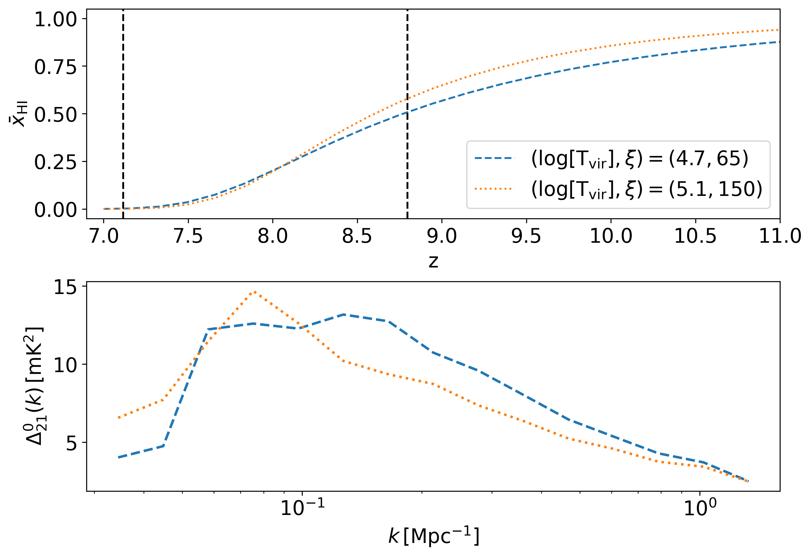
Figure 1: Top panel: The global ionization fraction of the IGM for $({\rm log[T_{vir}]},\xi)=(4.7,65)$ (blue dashed line) and for $({\rm log[T_{vir}]},\xi)=(5.1,150)$ (yellow dotted line). The black vertical dashed lines denote the $z=7.1$ and $z=8.8$ boundaries, which we use for the visibility simulation. Bottom panel: The spherically averaged 1D power spectrum of the brightness temperature field defined in Equation 10 for the $z=7.1-8.8$ lightcone.

An important aspect of our work is to illustrate the constraining power of the power spectrum multipoles for EoR parameters. Therefore, we choose two different sets of EoR parameters $({\rm log_{10}[T_{vir}/K]},\xi)$, which produce an almost identical global ionization history as well as a similar spherically averaged 1D power spectrum for comparison. Specifically, we choose $({\rm log_{10}[T_{vir}/K]},\xi)=(4.7,65),\,(5.1,150)$ to produce two sets of reionization lightcones. This is similar to the “faint galaxies” and “bright galaxies” models presented in Greig & Mesinger (2018). For simplicity, we use the same names for the two models we are considering. Lower values of $({\rm log_{10}[T_{vir}/K]},\xi)$ mean that the reionization process is driven by fainter, more numerous sources, and vice versa. The evolution of the global ionization fraction and the 1D monopole power spectrum along the observation lightcone are presented in Figure 1 for reference. We note that, in our simulation, reionization is almost complete at $z\sim 7.0$, which is faster than what has been suggested by current measurements (e.g. Bosman et al. 2022; Greig et al. 2024b). As discussed later in Section 2.2, we focus on the redshift range of $z\sim 7.1-8.8$ and thus a faster reionization produces larger anisotropic effects along the lightcone, which is ideal for presenting the case of comparing the constraining power of the monopole and the multipoles.

2.2 The interferometric observation

In this section, we present the simulation of visibility data using the configurations of the SKA-Low array. The SKA-Low array will be located at the Murchison Radio-astronomy Observatory (MRO), sharing the location with its precursor, the Murchison Widefield Array (MWA; Tingay et al. 2013). SKA-Low is capable of measuring the 21 cm signal from 50 MHz to 350 MHz, covering $z\sim 3-25$. The radio environment at the MRO provides a relatively clean frequency range of 140-200 MHz for EoR measurements (Offringa et al., 2015; Sokolowski et al., 2015). We choose the sub-band of 145-175 MHz, corresponding to the redshift range of $z\sim 7.1-8.8$ towards the later stage of the EoR when more than half of the IGM is ionized (Davies et al., 2018). The channel bandwidth is to set to 200 kHz, corresponding to the line-of-sight resolution of $k_{\parallel}\lesssim 1\,{\rm Mpc}^{-1}$. While the frequency resolution of SKA-Low will be finer than 200 kHz, the nonlinear scales $k_{\parallel}>1\,{\rm Mpc}^{-1}$ are hard to model and beyond the scope of this work. The 21 cm lightcone is smoothed along the line-of-sight to match the frequency resolution.

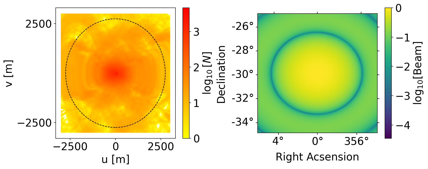
Figure 2: Left panel: The baseline distribution of the simulated tracking observation for SKA-Low. The grid size is chosen to be $(6\,{\rm m})^{2}$ for illustration and only the central area of $(3000\,{\rm m})^{2}$ is shown. The dashed circle indicates the $k_{\perp}\sim 1\,{\rm Mpc^{-1}}$ boundary within which the power spectra are calculated. Right panel: The instrument power beam of SKA-Low around the pointing centre.

We use the oskar package (Mort et al., 2010) to simulate the interferometric observations, with the telescope configuration following the latest official SKAO data challenge. The pointing centre is set to be near the EoR0 field (Lynch et al., 2021) at (RA=0 deg, Dec=-30 deg). The $u$-$v$ coverage of the baseline distribution is simulated with a tracking observation of 12 hrs with a time resolution of 10 s. The baseline distribution and the power beam are shown in Figure 2 for reference.

The standard deviation of the Gaussian thermal noise of visibilities follows the radiometer equation (e.g. Condon & Ransom 2016)

$$\sigma_{\rm N}=\frac{2k_{B}T_{\rm sys}}{A_{\rm e}\sqrt{\delta t\delta f}},$$ (5)

where $T_{\rm sys}$ is the system temperature, $A_{\rm e}$ is the effective collecting area of the antenna, $\delta t=10\,$s is the time resolution and $\delta f=200$ kHz is the channel bandwidth. In this paper, we aim to provide forecasts for power spectrum multipole measurements of a deep observation with coherent averaging of multiple nights. For a total integration time of $t_{\rm tot}$, the thermal noise amplitude for each baseline is scaled so that

$$\sigma_{\rm N}^{\rm avg}=\sigma_{\rm N}\sqrt{\frac{t_{\rm n}}{t_{\rm tot}}},$$ (6)

where $t_{\rm n}=12\,$hrs is the observation time of one night. In this paper, we follow the anticipated performance of SKA-Low in Braun et al. (2019) to produce the thermal noise. The natural sensitivity of the instrument is set to be $A_{\rm e}/T_{\rm sys}=[1.052,1.119,1.159,1.171,1.190]\,{\rm m^{2}/K}$ at $[140,150,160,170,180]$ MHz, and the amplitudes at each frequency channels are linearly interpolated. The total observation time is chosen to be $t_{\rm tot}=120\,$hrs. The choice of integration time of 120 hrs is relatively conservative, as the EoR0 field will potentially be observed for $>1000$ hrs. We note that, a large amount of data loss is expected for future surveys due to radio frequency interference (RFI) flagging. It is also common in data analysis to cross-correlate different time blocks to reduce systematic effects (e.g. Abdurashidova et al. 2022; Paul et al. 2023), which effective reduces the integration time by half. Overall, we expect $t_{\rm tot}=120\,$hrs to be a reasonable lower limit for future SKA-Low observations of one deep field.

As a preliminary study into the detectability and constraining power of EoR multipoles, simulating observational systematics is beyond the scope of our work. In particular, we assume that foreground contamination can be avoided by applying a horizon criterion so that

$$k_{\parallel}>c_{k}k_{\perp},$$ (7)

where the position of the wedge $c_{k}$ is determined by a characteristic angular scale $\theta_{0}$ so that (Liu et al., 2014)

$$c_{k}=\frac{H(z)D_{c}(z)\theta_{0}}{c(1+z)},$$ (8)

where $D_{c}(z)$ is the comoving distance. We choose $\theta_{0}=\sqrt{\Omega_{\rm beam}}$ following Chen et al. (2023b) which gives $c_{k}=0.28$, where $\Omega_{\rm beam}$ is the beam area calculated using the power beam shown in Figure 2. As the 21 cm signal during the EoR is anisotropic, the power spectrum averaged above the foreground wedge is biased compared to the spherical average (Jensen et al., 2016). It also leads to bias in the multipoles, inducing effective mode-mixing in the 1D multipole power spectra (Raut et al., 2018). In this paper, we refer to the average above the foreground wedge as “spherical average” for simplicity. The partition into clustering wedges discussed in Section 3.4 is performed above the foreground wedge instead of using the entire cylindrical $\bm{k}$-space.

Several observational effects induce foreground leakage into the observation window above the wedge. For example, chromatic data excision due to narrow-band RFI will cause foreground spillover (Wilensky et al., 2022). Calibration errors also introduce foreground scatter into high delay (e.g. Barry et al. 2016; Byrne et al. 2019). While it is not discussed in this paper, we note that the systematic effects can be partially mitigated in the quadratic estimator formalism, for example by including the foreground cleaning operation in the weighting matrix $\mathbf{R}$ (e.g. Kern & Liu 2021; Chen et al. 2023a, b).

3 Advantages of multipoles and clustering wedges

3.1 Power spectrum multipoles

In this section, we use the simulations described above to demonstrate the advantages of using multipoles as summary statistics for EoR surveys. Using power spectrum multipoles allows us to extract information from anisotropy and to probe the evolution of the EoR along the lightcone. Furthermore, the advantage of partitioning the measurements into clustering wedges is illustrated. For simplicity, when not specifically mentioned, the results shown correspond to the simulation using the faint model defined in Section 2.1.

In the flat-sky and plane-parallel limit, the power spectrum multipole of order $\ell$ in a clustering wedge can be written as (e.g. Scoccimarro 2015)

$$P^{\ell}_{21}(k)=\frac{2\ell+1}{\mu_{1}-\mu_{0}}\int^{\mu_{1}}_{\mu_{0}}{\rm d}\mu\,\mathcal{P}_{\ell}(\mu)\,P_{21}(\bm{k}),$$ (9)

where $k=|\bm{k}|$ is the mode of the 3D wavenumber vector, $\mu=k_{\parallel}/k$, $\mu_{0}$ and $\mu_{1}$ are the lower and upper limits of the clustering wedge, $\mathcal{P}_{\ell}$ is the Legendre polynomial, and $P_{21}(\bm{k})\equiv P_{21}(k,\mu)$ is the anisotropic 21 cm power spectrum. For illustration, we also use the “dimensionless” power spectrum

$$\Delta^{\ell}_{21}(k)=\frac{k^{3}}{2\pi^{2}}P^{\ell}_{21}(k).$$ (10)

The 3D multipoles are averaged into 1D $k$-bins. We choose the spacing to be logarithmically distributed from $0.05\,{\rm Mpc^{-1}}$ to $1\,{\rm Mpc^{-1}}$ with 20 bins. We consider $\ell=0,2,4$ in this paper. Unless specified otherwise, all power spectra are calculated with the inverse noise covariance weighted, baseline-sampled 3D bandpowers using the quadratic estimator formalism described in Appendix A.

In order to understand the information content of the multipoles, we also need to compute the covariance of the power spectra. While the noise covariance can be analytically calculated (see Appendix A), the signal itself is non-Gaussian and its covariance is difficult to quantify as it requires the computation of high-order correlations (Shaw et al., 2020). Instead, we use the jackknife method and calculate the signal covariance directly from the simulation lightcone. The lightcone is resampled 25 times along the transverse direction, each with a sub-area of $(320\,{\rm Mpc})^{2}$ taken out. The conversion from delay power spectrum to the 21 cm temperature power spectrum is susceptible to the lightcone effects, the plane-parallel approximation, and the treatment of the primary beam. For the results shown in this paper, we use the measured power spectra from visibility data, and ignore the systematic biases of the estimation. We note that, simulation-based inference (e.g. Zhao et al. 2022; Greig et al. 2024a) can be used to circumvent these problems, as it does not require an explicit likelihood and takes into account systematic effects through forward-modelling. The detailed treatment of an inference framework to be used on real data is beyond the scope of our work.

3.2 Information on anisotropy

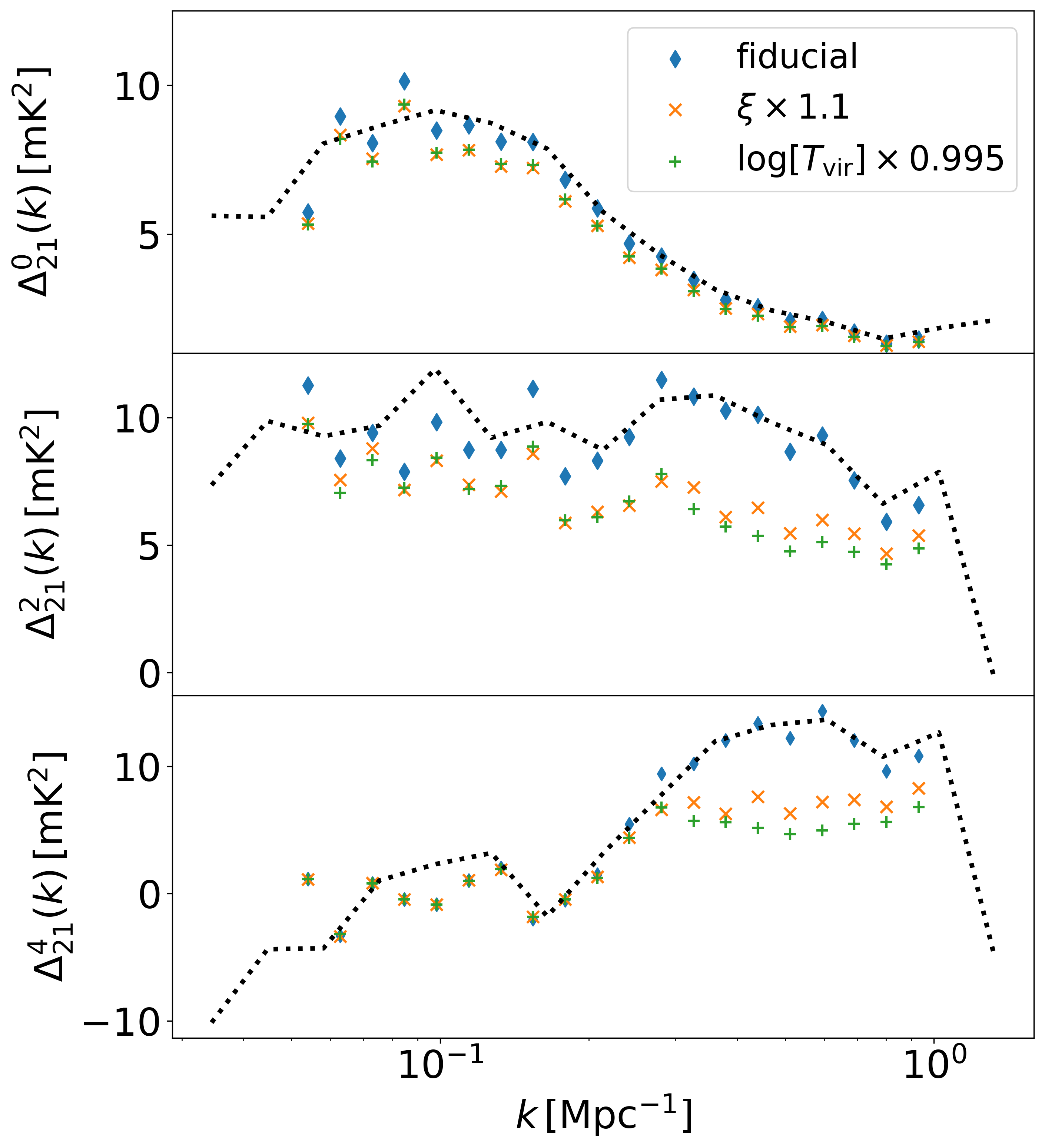
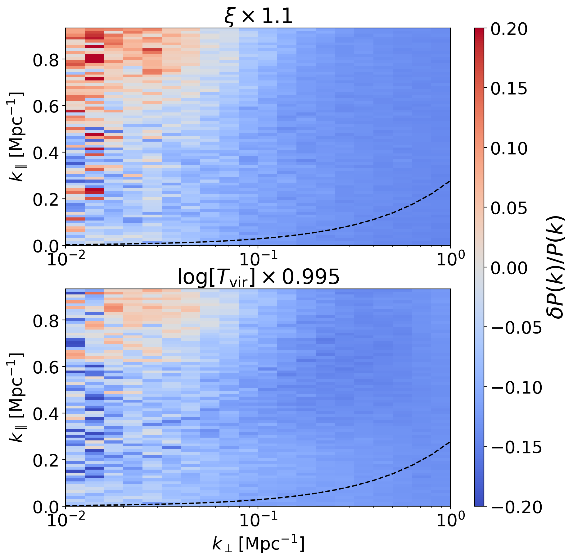
Figure 3: Top panel: The dimensionless power spectrum multipoles $\Delta^{0,2,4}_{21}(k)$ for the fiducial faint model (’fiducial’), the model with $\xi$ being 10% higher than the fiducial value (“$\xi\times 1.1$”), and the model with $\log[T_{\rm vir}]$ being 0.5% lower than the fiducial value (“$\log[T_{\rm vir}]\times 0.995$”). The latter two cases show very similar amplitudes for $\Delta^{0}_{21}(k)$, suggesting a degeneracy between the model parameters in the 1D monopole ($\ell=0$). The degeneracy is broken at higher $\ell$. The power spectrum of the input signal is shown in black dotted line for reference. Bottom panel: The fractional differences in the cylindrical power spectrum for the “$\xi\times 1.1$” and “$\log[T_{\rm vir}]\times 0.995$” models compared to the fiducial. Values larger than 0.2 are set to 0.2 and values smaller than -0.2 are set to -0.2 for better visualization.

The fluctuation of the 21 cm signal, as described by Equation 2, is determined by the multiplication of the ionization field, the spin temperature, the matter density field and the velocity field. While quantities such as the velocity field (e.g. Chapman & Santos 2019) and the spin temperature (e.g. Schaeffer et al. 2024) have a sizeable impact on the 21 cm power spectrum, the features of the fluctuation are mostly influenced by the matter density on large cosmological scales and the ionization field on small scales (Georgiev et al., 2022). Particularly, after the beginning of the percolation of the ionization bubbles, the ionization field becomes highly non-Gaussian (e.g. Shimabukuro et al. 2015) and non-linear (e.g. Hassan et al. 2016). As a result, the evolution of ionization bubbles along the line-of-sight induces anisotropy into the 21 cm power spectrum. The anisotropy can be captured in the cylindrical power spectrum. However, observational effects such as beam attenuation and frequency-dependent sampling create mode-mixing of different $\bm{k}$-modes, making it difficult to accurately measure the signal and its covariance in fine cylindrical $\bm{k}$-bins. Alternatively, power spectrum multipoles can be used for measuring the anisotropy.

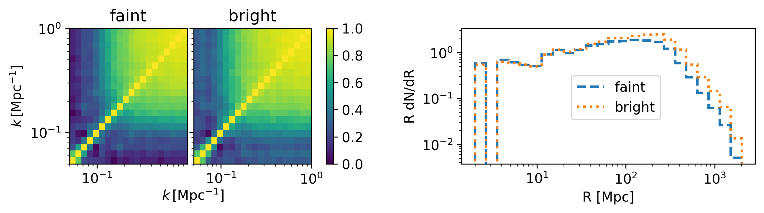
Figure 4: Left panel: The correlation matrix of the power spectrum monopole for the faint and bright models. Right panel: Bubble size distribution of the ionization field lightcone the for faint and bright models. The bubble sizes are calculated using the mean-free-path method and only completely ionized cells are considered.

For the spherically averaged power spectrum monopole, anisotropic information is lost, leading to obscurity in the interpretation of the amplitude of the signal. The lack of distinguishing power in the 1D monopole is illustrated in the upper panel of Figure 3. For the cases of increasing $\xi$ and decreasing $\log T_{\rm vir}$, the changes in the power spectrum amplitude are similar. This leads to a potential degeneracy between the model parameters, and indicates the limitations in the constraining power from monopole. On the other hand, as shown in the lower panel of Figure 3, the differences in the cylindrical power spectrum contain information on the model parameters. The constraining power is then reflected in the higher order multipoles $\ell=2$ and $\ell=4$. Increasing $\xi$ and decreasing $\log T_{\rm vir}$ lead to changes in the multipole power spectra with different structures. The differences are visible at all scales in the quadrupole, which can also be seen in the hexadecapole at small scales $k\gtrsim 0.3\,{\rm Mpc^{-1}}$.

3.3 Decorrelation of small-scale measurements

The patchiness of ionization bubbles during the EoR breaks the tracing of the brightness temperature field to the density field. As a result, at small scales the temperature power spectrum is highly correlated towards the end of reionization (e.g. Mondal et al. 2017). This is due to the fact that the signal is dominated by correlation within the same ionized structure at scales smaller than the typical size of the bubbles.

To illustrate this correlation, we show the correlation matrix of the monopole in Figure 4 for both the faint and bright models. For the faint model, the power spectrum signal is highly correlated at relatively small scales $k\gtrsim 0.2\,{\rm Mpc^{-1}}$. The monopole power spectrum is even more correlated for the bright model, especially on the large scales. The small-scale correlation indicates that the fluctuations of the ionization field are dominating the signal. To further establish the connection between the structures of the bubbles and the power spectrum correlation, we show the bubble size distribution for both faint and bright models in the right panel of Figure 4. The bubble size distribution is calculated using the mean-free-path method (Mesinger & Furlanetto, 2007) and only cells that are completely ionized are counted into the bubble sizes. Due to the fact that the reionization process is driven by brighter and less numerous sources in the bright model, there are more large bubbles in the bright model than in the faint model which can be seen in Figure 4. The increase in bubble sizes corresponds to the stronger correlation at large scales, verifying our conclusion on the connection between bubble sizes and signal correlation.

As the signal becomes completely correlated at small scales $k\sim 0.3\,{\rm Mpc^{-1}}$, the constraining power of the monopole on EoR parameters is severely limited. Although SKA-Low will be able to probe a wide range of scales, the extraction of information from measurements of the monopole is not sufficient. For forthcoming surveys, this issue may be compounded by the fact that shorter baselines are more susceptible to observational systematics (e.g. Amiri et al. 2023; Paul et al. 2023), leading to further signal loss. Alternative summary statistics that can probe small scales are thus called for.

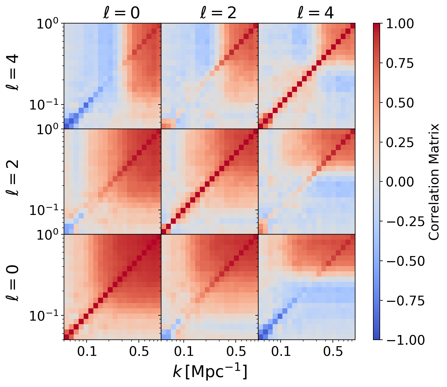
Figure 5: The correlation matrix of the power spectrum multipoles of the faint model. The signal is strongly correlated at $\ell=0$ (the monopole) on small scales $k\gtrsim 0.2\,{\rm Mpc^{-1}}$. The correlation becomes weaker at higher $\ell$.

In order to recover information from the small scale measurements, we can utilise higher-order multipoles. As we have shown in Section 3.1, the multipoles probe the evolution of the signal along the line-of-sight, subsequently disentangling the signal at smaller scales. In Figure 5, we show the correlation matrix for the multipole data vector including $\ell=0,2,4$. For the quadrupole, the signal completely decorrelates at large scales $k\lesssim 0.1\,{\rm Mpc^{-1}}$ and becomes less correlated compared to the monopole at $k\gtrsim 0.1\,{\rm Mpc^{-1}}$. For the hexadecapole, the correlation is even weaker and the signal only becomes correlated at $k\gtrsim 0.5\,{\rm Mpc^{-1}}$. Combined with the fact that the multipoles can distinguish changes in the reionization parameters as shown in Figure 3, this indicates that including the quadrupole and the hexadecapole will significantly increase the information content of 21 cm surveys.

The cross-correlation between $P^{\ell=0}_{21}$ and $P^{\ell=4}_{21}$ exhibits a transition from anticorrelation to correlation as shown in Figure 5. This is due to the baseline distribution leading to different sampling of the cylindrical $k$-space at different scales, which we discuss next.

3.4 Non-uniform sampling from baseline distribution

The $\bm{k}$-modes measured in a 21 cm survey are determined by the distribution of the interferometric baselines. For redundant arrays like HERA, specific $|\bm{k}_{\perp}|$ modes will be densely sampled and the $k$-dependence of the measured power spectrum is mainly contributed by the line-of-sight direction (see e.g. DeBoer et al. 2017). SKA-Low will be able to cover various scales on the transverse plane. However, the sampling of the $\bm{k}_{\perp}$ space is not homogeneous, as the sensitivity of the array will concentrate around specific scales of interest. As a result, the 1D average of multipoles will have highly uneven sampling across the cylindrical $\bm{k}$-space.

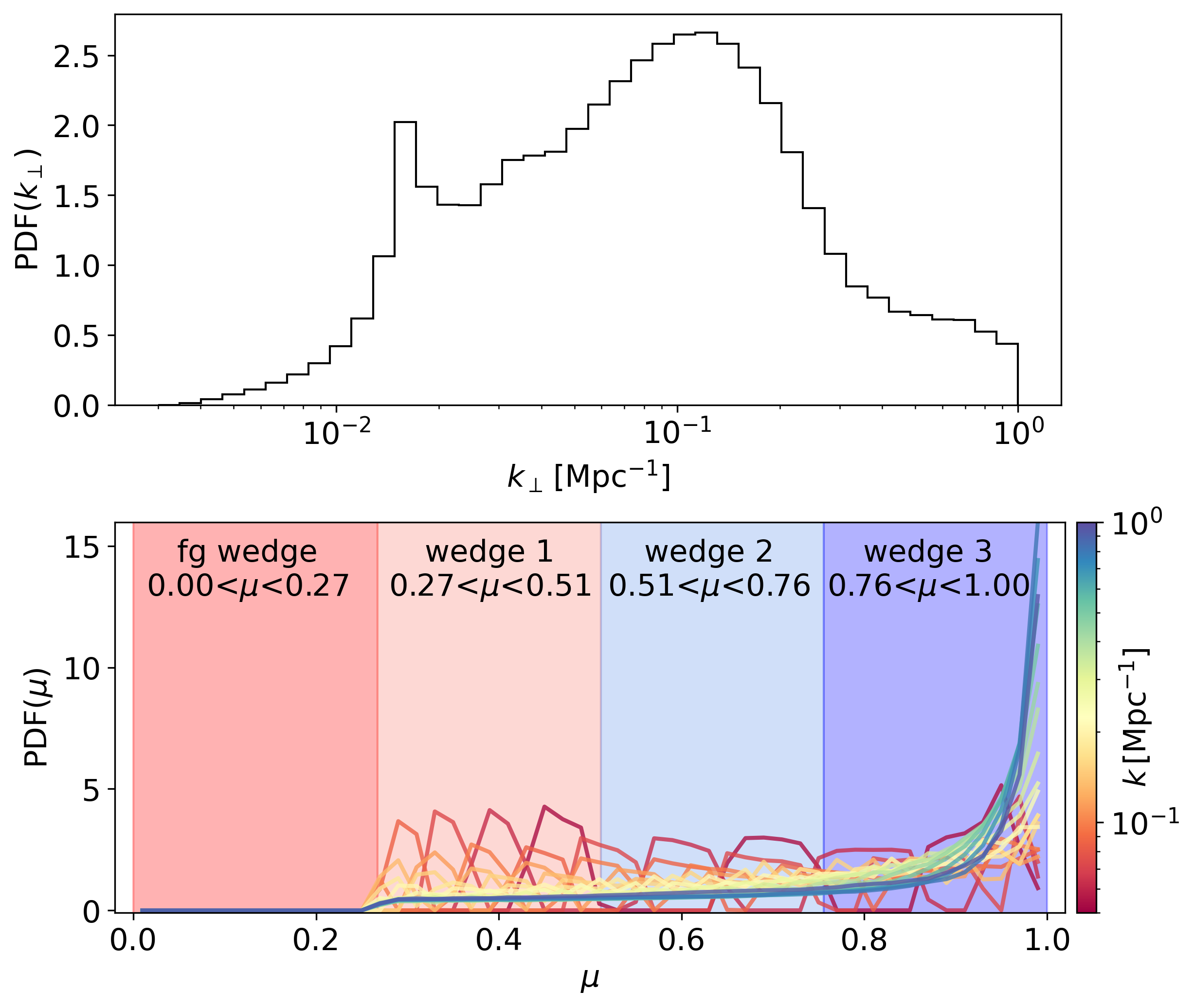
Figure 6: Top panel: The distribution function of the simulated SKA-Low baselines. The density of the baseline distribution peaks around $k_{\perp}\sim 0.1\,{\rm Mpc^{-1}}$. Bottom panel: The distribution function of $\mu$ in each 1D $k$-bin for spherically averaged power spectrum measurements. The distributions are colour-coded according to the $k$ value of each $k$-bin. The partitions of $\mu$-space into three different wedges are overlayed for reference. The foreground wedge is also shown. For large $k$, the sampling is skewed towards higher values of $\mu$ and is dominated almost entirely by $\mu\sim 1$ for $k\gtrsim 0.5\,{\rm Mpc^{-1}}$.

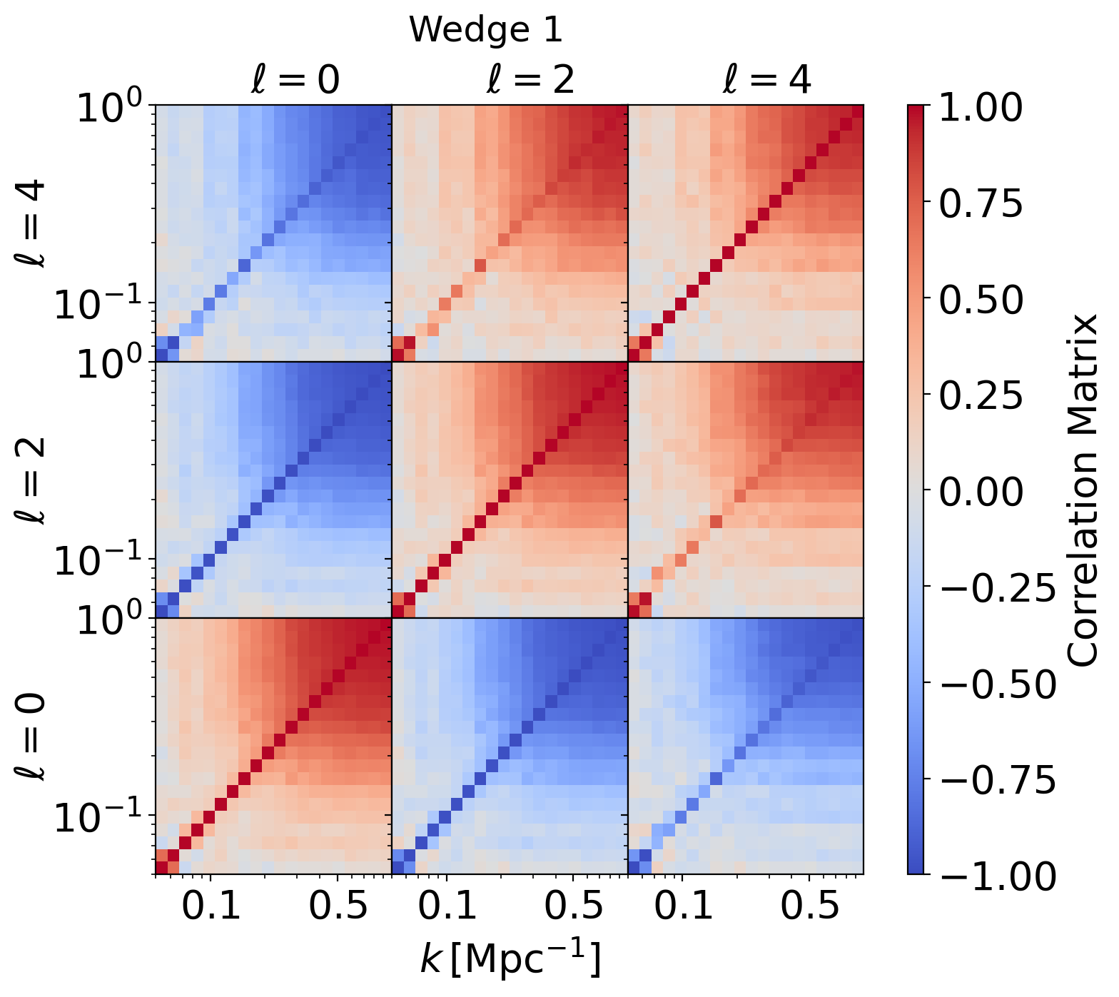
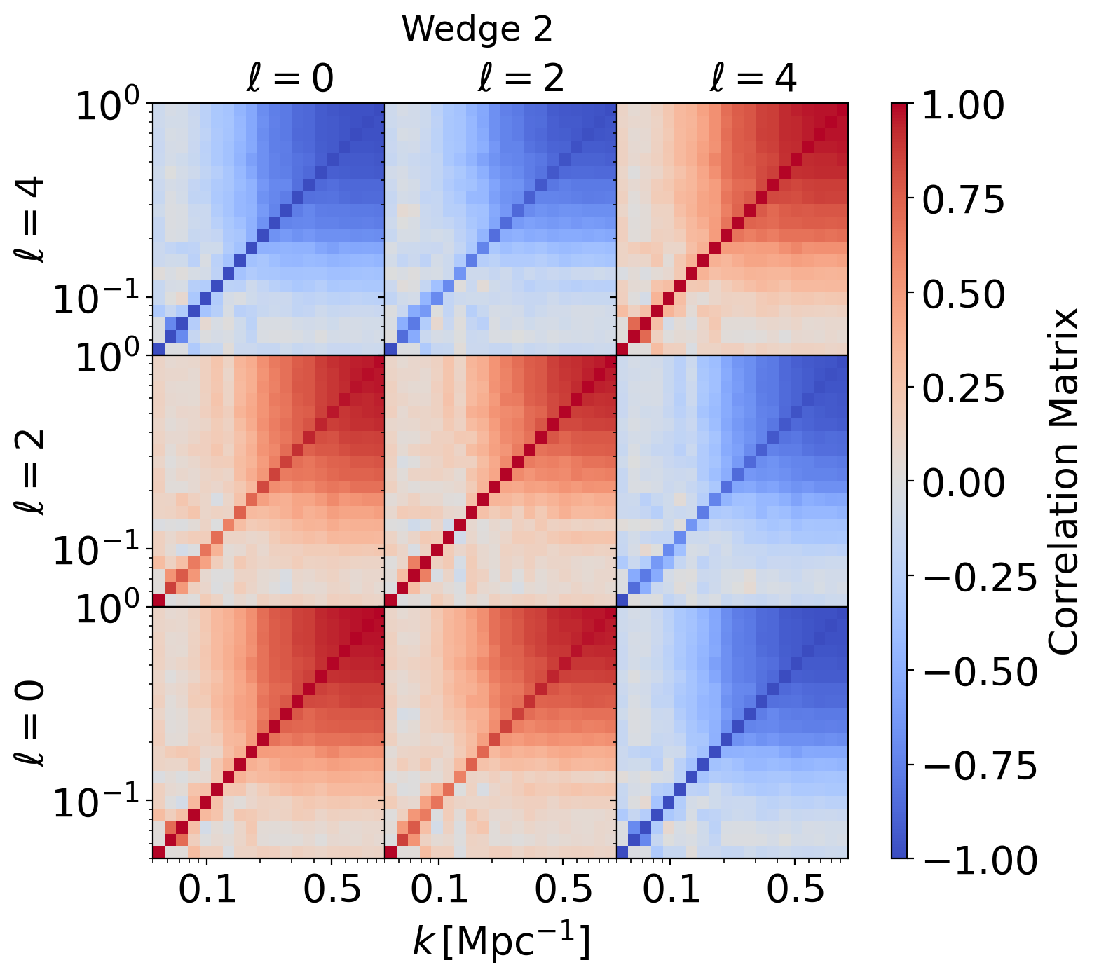
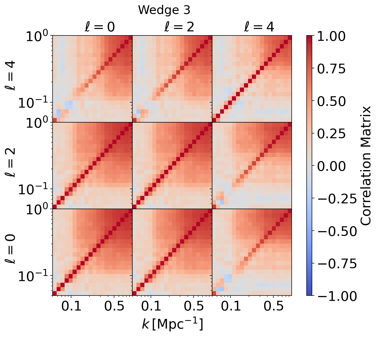
Figure 7: The correlation matrix of power spectrum multipoles for different clustering wedges. The numbering and positioning of the wedges are defined in Section 3.4 and shown in Figure 6.

In Figure 6, we show the 1D baseline distribution and the corresponding distribution function of $\mu$ for each 1D $k$-bin. The baseline distribution peaks around $k_{\perp}\sim 0.1\,{\rm Mpc^{-1}}$. Therefore, the sampling of $\mu$ is relatively even for large scales $k\lesssim 0.1\,{\rm Mpc^{-1}}$. On the other hand, the baseline distribution decreases sharply after the peak. For relatively small scales $k\gtrsim 0.1\,{\rm Mpc^{-1}}$, the contribution into the 1D power spectrum comes mainly from the large $k_{\parallel}$ region, skewing the distribution of $\mu$ towards higher values. The large deviation from uniformly sampled $\mu$ indicates loss of information, as spherically averaged power spectra will not be able to fully probe the $k_{\parallel}$-dependence of the signal and rather measures certain regions of large $\mu$.

To resolve the uneven sampling, we divide the $\mu$-region above the foreground wedge into three different clustering wedges shown in Figure 6. The foreground wedge is at $c_{k}=0.28$ and equivalently $\mu=0.267$. The $\bm{k}$-space above the foreground wedge is then split into three equally spaced regions of $\mu$. The partitioning resolves the uneven sampling by isolating less-sampled regions of $\mu$, leading to relatively even sampling in each clustering wedge. As previously mentioned in Section 3.3, one of the consequences of the uneven sampling is the transition from correlation to anticorrelation between the monopole and the hexadecapole as shown in Figure 5. As a comparison, we show the correlation matrix for the multipoles within each wedge in Figure 7. The transition disappears when the clustering wedges are used. We note that, due to the non-Gaussianity of the 21 cm signal leading to higher-order correlation (e.g. Majumdar et al. 2018), on small scales the $k$-modes are correlated between clustering wedges. The full correlation matrix including the cross-correlation between different wedges is shown in Figure 10 for reference.

Comparing the correlation of multipoles in wedges with the spherical average, we can see that in the wedge with the largest $\mu$, the multipole power spectra are less correlated. This is consistent with the fact that the $\bm{k}$-modes with higher $\mu$ probe small line-of-sight scales, providing more information on the evolution along the lightcone. In the spherical average, at lower $k$ the sample is uniform. At higher $k$, the sampling becomes heavily skewed towards the third wedge, and the difference in the sampling of $\mu$ at different $k$ leads to the structure in Figure 5.

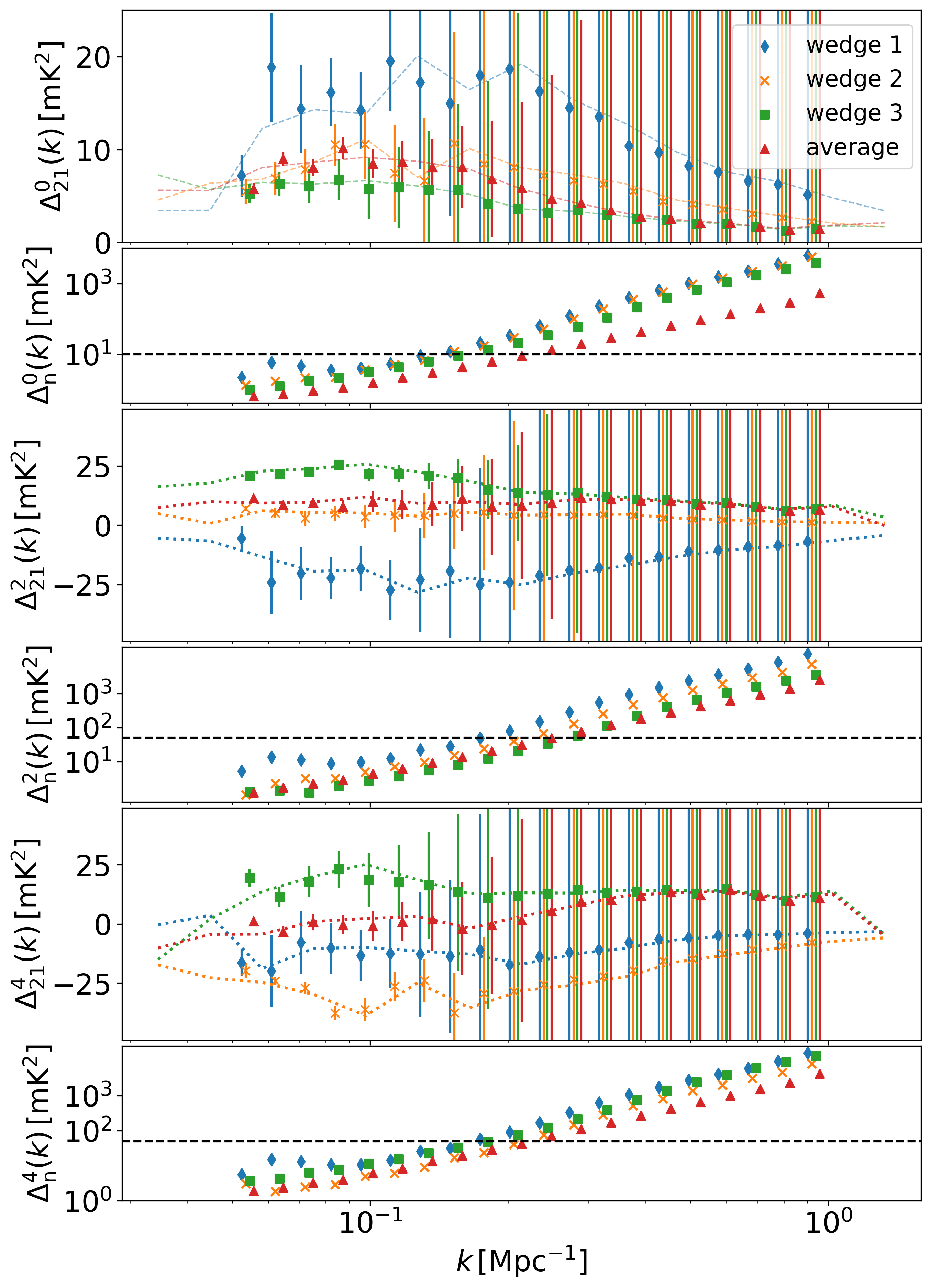
Figure 8: The forecasted measurements of the power spectrum multipoles for SKA-Low observations with 120 hrs of integration time. The panels from top to bottom show the measurements for $\ell=0$, $\ell=2$ and $\ell=4$. Measurements of each clustering wedge defined in Section 3.4 are shown together with the measurements of the spherically averaged power spectrum (“average”). The dotted lines denote the signal power spectrum with no errors. In the lower part of each panel, the amplitudes of the measurements errors, denoted as $\Delta^{\ell}_{n}$, are also shown for reference. The black dashed line denotes a schematic upper limit for the noise level, above which the measurements no longer contain information. The centres of the $k$-bins are slightly shifted for better visualization.

4 Parameter Constraints

4.1 Fisher matrix

In this section, we forecast the constraining power of power spectrum multipoles for SKA-Low. The information content in summary statistics can be quantified via the Fisher matrix formalism (see e.g. Euclid Collaboration et al. 2020)

$$\mathbf{F}_{\alpha\beta}=\frac{1}{2}{\rm tr}\bigg{[}\frac{\partial\mathbf{C}}{\partial\theta_{\alpha}}\mathbf{C}^{-1}\frac{\partial\mathbf{C}}{\partial\theta_{\beta}}\mathbf{C}^{-1}\bigg{]}+\frac{\partial\bm{\mu}^{\rm T}}{\partial\theta_{\alpha}}\mathbf{C}^{-1}\frac{\partial\bm{\mu}}{\partial\theta_{\beta}},$$ (11)

where $\rm tr$ denotes the trace of a matrix, $\bm{\mu}$ is the assemble average of the data vector of the summary statistics, $\mathbf{C}$ is the data covariance, ^T denotes the transpose operation and $\{\theta\}$ is the parameter set. The inverse of the Fisher matrix gives a lower bound of the error covariance of parameter inference (Cramér, 1999; Rao, 1992)

$$\mathbf{C}_{\theta}=\mathbf{F}^{-1}.$$ (12)

The $1\sigma$ measurement error of a parameter $\alpha$ can then be written as

$$\sigma_{\alpha}=\sqrt{(\mathbf{C}_{\theta})_{\alpha\alpha}}.$$ (13)

The correlation coefficient between two parameters $\alpha$ and $\beta$ can be written as

$$\rho_{\alpha\beta}=\frac{(\mathbf{C}_{\theta})_{\alpha\beta}}{\sqrt{(\mathbf{C}_{\theta})_{\alpha\alpha}(\mathbf{C}_{\theta})_{\beta\beta}}}.$$ (14)

To calculate the partial derivative of the power spectrum multipoles and the data covariance, we run the EoR simulations with small changes to the input parameters, shifting the values of the parameters around the fiducial values. We fix the initial condition when varying the EoR parameters in each realization, and average the calculated derivatives over 10 different realizations, after which we find that convergence has been reached. We test the choice of step size between $0.1\%$ to $5\%$ and choose it to be $1\%$ to calculate the derivatives. While we find the correlation between the parameters vary slightly, the forecasts for parameter constraints discussed in Section 4 are consistent with different step sizes.

In large scale structure surveys, it is often assumed that either the mean of the data vector is zero or the derivatives of the data covariance is negligible (e.g. Euclid Collaboration et al. 2020). We find that in our case, both terms on the r.h.s of Equation 11 have non-negligible contribution, consistent with the findings in Prelogović & Mesinger (2024).

The total data covariance matrix is the sum of signal covariance and noise covariance. As mentioned in Section 3.1, we use the quadratic estimator formalism to calculate the noise covariance which is then added to the signal covariance. The amplitude of the thermal noise fluctuation is calculated assuming 120 hrs of integration time following Equation 5 as discussed in Section 2.2.

4.2 Detectability of multipoles

Using the total data covariance, we present the forecasts on the measurement errors of power spectrum multipoles for SKA-Low in Figure 8. To examine which scales can be probed by SKA-Low, we calculate a qualitative upper limit shown as the black dashed lines, above which the measurements provide negligible information. The limits are calculated using the maximum and the minimum of the multipoles in different wedges shown in Figure 8 and correspond to $\Delta^{0,2,4}_{\rm limit}=10,50,50\,{\rm mK^{2}}$. For reference, the forecasts for measurement errors for the spherically averaged power spectra are also shown in Figure 8.

For 120 hrs of integration time, SKA-Low will be able to measure the multipoles up to $k\sim 0.2\,{\rm Mpc^{-1}}$. Accurately modelling the data covariance is therefore essential, as the signal at small scales is non-Gaussian. Since the baseline distribution peaks around $k_{\perp}\sim 0.1\,{\rm Mpc^{-1}}$, sensitivities at smaller scales decrease sharply, and there is limited amount of information that can be extracted. For a complete, futuristic EoR survey, measurements down to $k\sim 1.0\,{\rm Mpc^{-1}}$ can be reached for $\sim 10,000$ hrs of integration time. We refrain from discussing such a scenario. As discussed later in Section 4.3, we find that per-cent level precision can be reached for $\sim 120\,$hrs. For accurate forecasts of $\sim 10,000$ hrs, the requirements on the accurate modelling of the signal and its covariance will be very stringent, and are beyond the scope of this work.

4.3 Comparing the constraining powers of multipoles and wedges to the monopole

Using the calculated data covariance and the Fisher matrix formalism, we present the forecasts for constraints on EoR parameters for SKA-Low. In order to compare using multipoles as summary statistics with other approaches, we consider four scenarios: Using only the spherically averaged monopole (“mono+avg”), the spherically averaged multipoles (“multi+avg”), the monopole in clustering wedges (“mono+wedge”) and the multipoles in clustering wedges (“multi+wedge”). Both the faint and the bright models are considered, in order to demonstrate the constraining power for different types of reionization morphology.

model	faint					bright
parameter	fid	mono+avg	multi+avg	mono+wedge	multi+wedge	fid	mono+avg	multi+avg	mono+wedge	multi+wedge
$(\sigma)\xi$	65	8.145	3.823	4.310	2.873	150	2.624	1.229	1.509	0.839
$(\sigma){\rm log}_{10}[T_{\rm vir}/{\rm K}]$	4.7	0.064	0.031	0.036	0.024	5.1	0.033	0.017	0.019	0.013
$\rho_{\zeta{\rm log}T_{\rm vir}}$	/	0.953	0.890	0.913	0.879	/	0.110	-0.096	-0.036	-0.149
${\rm det}[\mathcal{F}]$	/	40.41	335.20	256.19	958.42	/	138.66	2249.04	1217.63	8438.86

Table 1: Forecasts for the constraining power of 21 cm surveys using SKA-Low for EoR model inference. Two parameters, the ionization efficiency $\xi$ and the minimum virial temperature $(\sigma){\rm log}_{10}[T_{\rm vir}/{\rm K}]$, are considered here. The correlation coefficient of the two parameters, $\rho_{\zeta{\rm log}T_{\rm vir}}$, and the determinant of the Fisher matrix, ${\rm det}[\mathcal{F}]$, are also shown for reference. The faint and bright models are as defined in Section 2.1. From left to right, each column shows the fiducial value, the forecasts for using only the spherically averaged monopole (“mono+avg”), the spherically averaged multipoles (“multi+avg”), the monopole in clustering wedges (“mono+wedge”) and the multipoles in clustering wedges (“multi+wedge”).

In Table 1, we list the forecasts for the $1\sigma$ measurement errors of the EoR parameters. Apart from the $1\sigma$ confidence interval, we also show the correlation coefficient of the two parameters as a reference for parameter degeneracy, as well as the Fisher information volume. For both models, we can see that the constraining power of SKA-Low increases significantly by including higher-order multipoles and using clustering wedges. The measurement errors are lower by a factor of $\sim 2$ when either multipoles or clustering wedges are included. The improvement suggests that a significant amount of information lies in the anisotropy of the 21 cm power spectrum. Combining the power spectrum multipoles with clustering wedges, we find that the measurement errors decrease by a factor of $\sim 3$ comparing to using spherically averaged monopole. For a survey of $120\,$hrs, the SKA-Low will be able to constrain the ionization efficiency $\xi$ up to $\sim 3\%$ precision and the minimum virial temperature ${\rm log}[T_{\rm vir}]$ up to $\lesssim 1\%$ precision.

For the faint model, we find that the parameters are highly degenerate, as illustrated in Figure 3. Including the multipoles yields a slight improvement in resolving the degeneracy. The lack of improvement can be explained by the lack of information on small scales. The measurements on scales $k\gtrsim 0.1\,{\rm Mpc^{-1}}$ are expected to probe small scales along line-of-sight, which provides information on the evolution of EoR. For the noise level assumed in this work, the small scales cannot be measured with high precision and thus the degeneracy persists. For the bright model, we find no significant correlation between the parameters. We visualise the $1\sigma$ confidence region of our forecasts in Figure 9.

The constraints on the EoR parameters are much more stringent for the bright model. This is due to the fact that the bright model adopts extreme fiducial values for the model parameters. As reionization is driven by massive and bright sources in the bright model, the variation in the model parameters produces bigger changes in the power spectra comparing to the faint model.

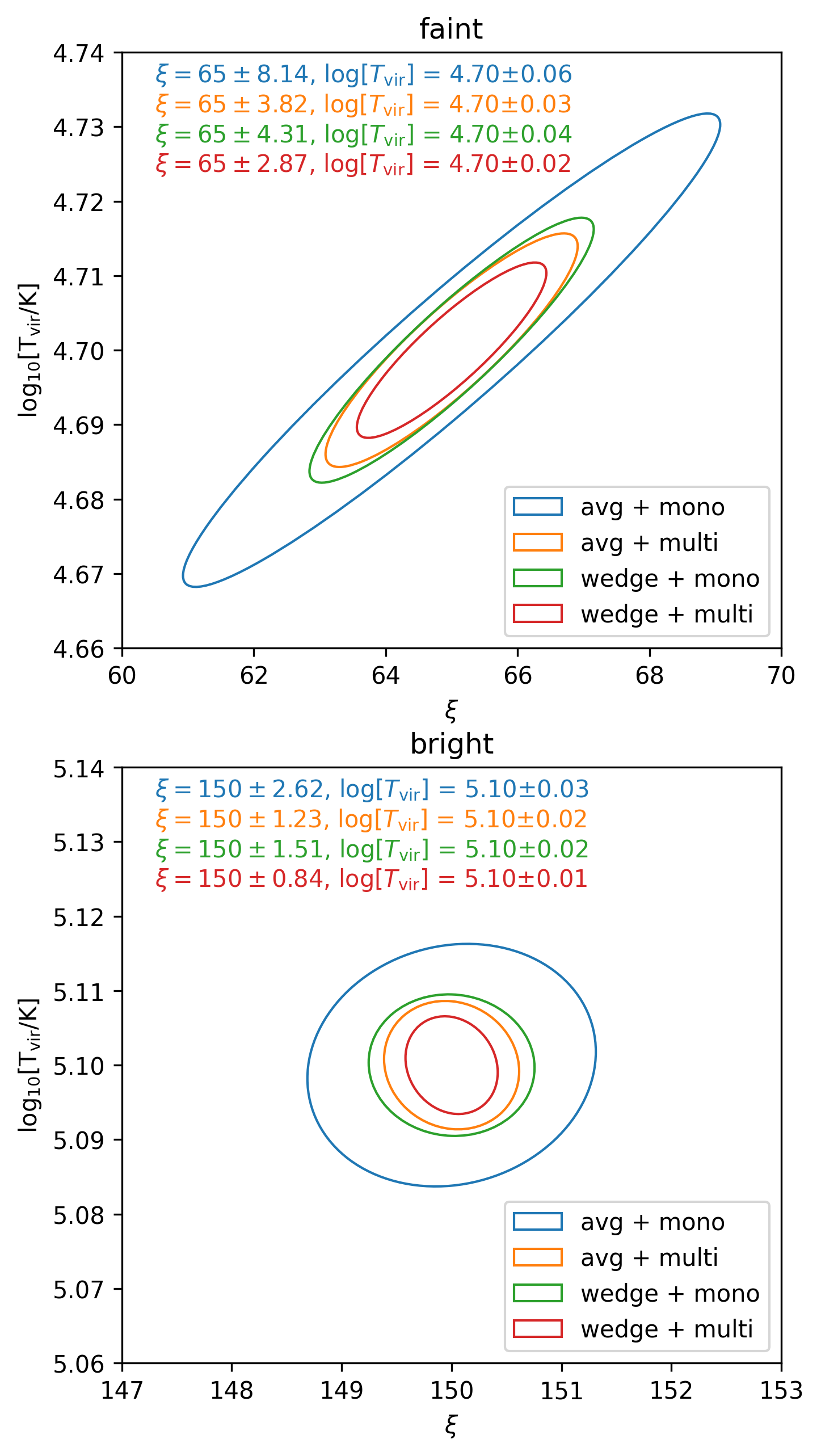
Figure 9: The forecasts on the $1\sigma$ confidence region of the parameter constraints from SKA-Low for the faint (top panel) and bright (bottom panel) model. Different summary statistics discussed in Section 4.3 are colour-coded and the resulting confidence intervals are listed on the top left corner of each panel.

In conclusion, we find that for SKA-Low, a 21 cm survey with $120\,$hrs of integration time will be able to measure the 21 cm power spectrum with high sensitivity. The visibilities can be summarised into power spectrum multipoles in clustering wedges, and can be used to accurately constrain the EoR parameters.

5 Conclusions

In this paper, we explore the advantages of using power spectrum multipoles and clustering wedges as summary statistics over using the spherically averaged monopole power spectrum for EoR measurements. In particular, we comprehensively demonstrate where additional information arises in the power spectrum multipoles and in the partition of the cylindrical $\bm{k}$-space. We then present forecasts for parameter constraints using multipole power spectra and clustering wedges for SKA-Low observations of redshift range $z\sim 7.1-8.8$.

We confirm the importance of extracting information from power spectrum anisotropy. Through simulating mock 21 cm observations for future SKA-Low surveys using different model parameters for the EoR, we verify that the 1D monopole power spectrum is not optimal in distinguishing physical models of reionization, as it averages over the entire $\bm{k}$-space without retaining the anisotropic information of the 21 cm signal. We point out that power spectrum multipoles provide a direct summary of the anisotropic 21 cm cylindrical power spectrum. There is visible improvement in the constraining power from the amplitude of the power spectra when multipoles are included. Small scale measurements of multipoles probe small-scale evolution along the line-of-sight and contain information for constraining EoR parameters.

EoR signals at small scales are dominated by the morphology of the ionization bubbles. The resulting monopole power spectrum is therefore highly correlated, especially for the latter stage of reionization considered in this work. We quantify the covariance of the signal with a large suite of simulations of the reionization lightcone, and find that small scales $k\gtrsim 0.2\,{\rm Mpc^{-1}}$ are almost completely correlated for the monopole. We verify that this correlation is indeed caused by the growth of ionization bubbles, as simulations with larger and fewer bubbles show stronger correlation at large scales. To our knowledge, we are the first to point out that this correlation can be disentangled by including the quadrupole and hexadecapole power spectra. The higher-order multipoles probe line-of-sight scales along which reionization evolve rapidly, providing information beyond the compressed 1D fluctuation.

The baseline distribution of a radio interferometer is not uniform. As a result, we find that for SKA-Low, the sampling in the cylindrical $\bm{k}$-space is skewed heavily towards large values of $\mu$ for scales $k\gtrsim 0.2\,{\rm Mpc^{-1}}$ when averaged into 1D power spectra. Therefore, measurements at large $k$ effectively only probe a small region of $\bm{k}$-space with high $k_{\parallel}$. This calls for the partitioning of $\bm{k}$-space into clustering wedges. Within each clustering wedge, the sampling of $\mu$ becomes relatively uniform. The power spectrum multipoles can then be used to measure the $k_{\parallel}$-dependence of the signal, optimally extracting information on the EoR. Accurate calculation of the signal covariance will be crucial for model inference, as there are significant contributions from higher-order correlations in the covariance matrix.

In order to estimate the constraining power of the multipoles and clustering wedges for the EoR, we perform Fisher matrix forecasts to quantify the error covariance of reionization parameters assuming $120\,$hrs of observation with SKA-Low. We find that on large scales $k\lesssim 0.1\,{\rm Mpc^{-1}}$, the multipole power spectra can be measured with relatively high precision. As a result, SKA-Low will be able to give stringent constraints on EoR parameters, with the measurement errors reaching $\lesssim 1\%$. Comparing to only using the spherically averaged monopole, the power spectrum multipoles in clustering wedges yield a factor of $\sim$3 improvement on parameter constraints. Due to the lack of sensitivity for scales $k\gtrsim 0.1\,{\rm Mpc^{-1}}$, the degeneracy between EoR parameters is only slightly resolved by including the multipoles. For a complete 21 cm survey with $\sim 10,000\,$hrs of integration time, SKA-Low will be able to probe into the small scales $k\sim 1\,{\rm Mpc^{-1}}$ where the multipoles can be used to further break the degeneracy.

Our work provides strong incentives for using power spectrum multipoles in clustering wedges in forthcoming EoR measurements. In addition to the advantages mentioned above, the multipoles are less susceptible to various observational systematic effects. Quantifying the covariance of the multipoles in different wedges from visibility data and using a conventional model inference framework with the multipoles are within the reach of the anticipated data quality in the near future. Robust model inference with the power spectrum multipoles and clustering wedges will provide crucial insights into the physics driving the cosmic reionization.

Data Availability

The scripts for simulating reionization lightcones are publically available as a github repository. The scripts for visibility simulation and the subsequent Fisher matrix analysis are not publicly available at the moment and will be shared on reasonable request to the corresponding author.

Appendix A Quadratic Estimator for Power Spectrum Multipoles

In this section, we discuss the quadratic estimator formalism used in this paper for power spectrum multipoles. The quadratic estimator for cosmological power spectra is well studied in the context of CMB (e.g. Tegmark 1997; Tegmark & de Oliveira-Costa 2001), galaxy clustering (e.g. Tegmark et al. 1998) and more recently in interferometric 21 cm observations (e.g. Liu & Tegmark 2011; Kern & Liu 2021). For this work, we follow the formalism in Kern & Liu (2021) and Chen et al. (2023a), and specify our estimator in the context of the delay power spectrum from visibilities. We then generalise it to power spectrum multipoles.

A radio interferometer measures the sky emission with baselines, i.e. pairs of antennas, as visibilities (Smirnov, 2011)

$$\begin{split}V(u,v,w,f)=\iint&\frac{{\rm d}l\,{\rm d}m}{\sqrt{1-l^{2}-m^{2}}}\,I(l,m,f)\,A(l,m,f)\\ \times&\,{\rm exp}\big{[}-2\pi(lu+mv+\sqrt{1-l^{2}-m^{2}}w)\big{]},\end{split}$$ (15)

where $I(l,m,f)$ is the flux density of the sky signal at frequency $f$ and angular coordinate on the sky $(l,m)$, and $A(l,m,f)$ is the power response of the instrument. For a pair of antennas, the distance vector between them, denoted as $\bm{b}$, can be written in East-North-Up (ENU) coordinate frame as

$$\bm{b}=\lambda(u,v,w)^{\rm T},$$ (16)

where $\rm T$ denotes the transpose operation and $\lambda$ is the observing wavelength.

For each instantaneous baseline, the visibilities across the frequency channels can be Fourier transformed so that

$$\tilde{V}(u,v,\eta)=\int{\rm d}f\,V(u,v,f)\,{\rm exp}\big{[}-2\pi\eta f\big{]}.$$ (17)

For the 21 cm signal, the coordinates $(u,v)$ reflect the angular scale in Fourier space while the delay time $\eta$ reflects the Fourier mode of density fluctuation along the line-of-sight:

$$\bm{k}_{\perp}=\frac{2\pi\bm{u}}{X}$$ (18)

$$k_{\parallel}=\frac{2\pi\eta}{Y},$$ (19)

where $\bm{u}=(u,v)^{\rm T}$.

For a bandpower in the $\alpha^{\rm th}$ $\bm{k}$-bin of a multipole moment $\ell$, which we denote as $p^{\ell}_{\alpha}$, the quadratic estimator can be written as

$$\hat{p}^{\ell}_{\alpha}=C_{\rm H\textsc{i}}\,\big{(}\mathbf{V}^{\dagger}\,\mathbf{E}_{\alpha}^{\ell}\,\mathbf{V}-\hat{b}^{\ell}_{\alpha}\big{)},$$ (20)

where $\mathbf{V}$ is the visibility data vector, $\dagger$ denotes the Hermitian transpose, $\mathbf{E}_{\alpha}^{\ell}$ is an estimation matrix discussed later and $\hat{b}^{\ell}_{\alpha}$ is the bias correction term. $C_{\rm H\textsc{i}}$ is a factor that converts the flux density to brightness temperature unit and renormalises the survey volume (Parsons et al., 2014)

$$C_{\rm H\textsc{i}}=\bigg{(}\frac{\lambda^{2}}{2k_{\rm B}}\bigg{)}^{2}\frac{X^{2}Y}{\Omega_{\rm ps}B},$$ (21)

where $\lambda$ is the observing frequency, $k_{\rm B}$ is the Boltamann constant, $X$ is the comoving distance of the 21 cm signal at the observing frequency, $B$ is the frequency bandwidth of the observation, and $\Omega_{\rm ps}$ is the power-squared beam area defined as

$$\Omega_{\rm ps}=\int{\rm d}l{\rm d}m|A(l,m)|^{2}.$$ (22)

$Y$ is the comoving length scale per frequency interval

$$Y=\frac{\lambda(1+z)}{H(z)},$$ (23)

where $z$ is the redshift of the 21 cm signal at the observing frequency, and $H(z)$ is the Hubble parameter.

The data vector comprises visibilities measured at each baseline at each time step in each frequency channel. For an ideal experiment where the data vector consists only of Hi signal and the beam response is unitary, the 21 cm power spectrum for $\bm{k}_{\alpha}$ can be written as (McQuinn et al., 2006; Parsons et al., 2012, 2014)

$$P_{\rm 21}(\bm{k}_{\alpha})=C_{\rm H\textsc{i}}|\tilde{V}^{\rm ideal}(u_{\alpha},v_{\alpha},\eta_{\alpha})|^{2}.$$ (24)

The power beam of the instrument is multiplied with the signal on the sky, and therefore convolves the signal in Fourier space. The mode-mixing can be written in the data vector as

$$\tilde{V}^{\ell}_{\alpha}=\sum_{\beta}\mathcal{M}^{\ell}_{\alpha\beta}\tilde{V}^{\ell,\rm ideal}_{\beta},\,\tilde{V}^{\ell}_{\alpha}=\tilde{V}^{\ell}(\bm{k}_{\alpha}),$$ (25)

where $\mathcal{M}^{\ell}_{\alpha\beta}$ is the mode-mixing matrix that can be calculated given the power beam, and $\tilde{V}^{\ell}_{\alpha}$ is the delay-transformed data vector for multipole $\ell$:

$$\tilde{\mathbf{V}}^{\ell}=\mathcal{F}_{\ell}\,\mathbf{V}.$$ (26)

$\mathcal{F}_{\ell}$ is the Fourier transformation kernel that transforms the visibility to multipole overdensity. In this paper, we consider $\ell=(0,2,4)$. $\mathcal{F}_{0}$ is simply the Discrete Fourier Transform kernel. For higher moments, in the flat-sky and plane-parallel limit we have (Scoccimarro, 2015)

$$\mathcal{F}_{2}=\frac{3}{2}{\rm diag}\big{[}\bm{\hat{k}}_{\parallel}^{2}\big{]}\mathcal{F}_{0}-\frac{1}{2}\mathcal{F}_{0},$$ (27)

$$\mathcal{F}_{4}=\frac{35}{8}{\rm diag}\big{[}\bm{\hat{k}}_{\parallel}^{4}\big{]}\mathcal{F}_{0}-\frac{5}{2}\mathcal{F}_{2}-\frac{7}{8}\mathcal{F}_{0},$$ (28)

where ${\rm diag}[]$ denotes the operation that diagonalises a vector into a matrix, $\bm{\hat{k}}_{\parallel}$ is a vector so that $\bm{\hat{k}}_{\parallel}^{\alpha}=\bm{\mu}^{\alpha}=k_{\parallel}^{\alpha}/|\bm{k}_{\alpha}|$.

Similar to Equation 24, we can then write down the estimator when the measurement is ideal:

$$\hat{p}^{\rm ideal,\ell}_{\alpha}=C_{\rm H\textsc{i}}\big{(}\tilde{V}^{\ell,\rm ideal}\big{)}^{\dagger}\,{\rm diag}\big{[}\bm{w}_{\alpha}\big{]}\,\tilde{V}^{\rm 0,ideal},$$ (29)

where $\bm{w}_{\alpha}$ is a selection vector with the $\alpha^{\rm th}$ element being 1 and all other elements 0.

We can then factorize the estimator of Equation 20 in a way that relates to the Fourier multipole overdensity

$$\begin{split}\langle\hat{p}^{\ell}_{\alpha}\rangle=&C_{\rm H\textsc{i}}\bigg{\langle}\big{(}\tilde{\mathbf{V}}^{\ell}\big{)}^{\dagger}\,\big{(}\mathcal{F}_{\ell}^{-1}\big{)}^{\dagger}\,\mathbf{E}^{\ell}_{\alpha}\mathcal{F}_{0}^{-1}\,\tilde{\mathbf{V}}^{0}\bigg{\rangle}\\ =&C_{\rm H\textsc{i}}\bigg{\langle}\big{(}\tilde{\mathbf{V}}^{\ell,\rm ideal}\big{)}^{\dagger}\,\big{(}\mathcal{M}^{\ell}\big{)}^{\dagger}\,\big{(}\mathcal{F}_{\ell}^{-1}\big{)}^{\dagger}\,\mathbf{E}^{\ell}_{\alpha}\,\mathcal{F}_{0}^{-1}\,\mathcal{M}^{0}\,\tilde{\mathbf{V}}^{0,\rm ideal}\bigg{\rangle}\\ =&C_{\rm H\textsc{i}}\,{\rm tr}\Big{[}\tilde{\mathbf{E}}^{\ell}_{\alpha}\big{\langle}\tilde{\mathbf{V}}^{0,\rm ideal}\,\big{(}\tilde{\mathbf{V}}^{\ell,\rm ideal}\big{)}^{\dagger}\big{\rangle}\Big{]},\end{split}$$ (30)

where the bias term is neglected for now, ${\rm tr}[]$ denotes the trace of a matrix and we have defined a mode-mixed Fourier space estimator

$$\tilde{\mathbf{E}}^{\ell}_{\alpha}=\big{(}\mathcal{M}^{\ell}\big{)}^{\dagger}\,\big{(}\mathcal{F}_{\ell}^{-1}\big{)}^{\dagger}\,\mathbf{E}^{\ell}_{\alpha}\,\mathcal{F}_{0}^{-1}\,\mathcal{M}^{0}.$$ (31)

Assuming that the 21 cm field does not correlate for different $\bm{k}$-modes, the covariance matrix of the ideal signal can be written as

$$C_{\rm H\textsc{i}}\big{\langle}\tilde{\mathbf{V}}^{0,\rm ideal}\,\big{(}\tilde{\mathbf{V}}^{\ell,\rm ideal}\big{)}^{\dagger}\big{\rangle}=\sum_{\beta}{\rm diag}\big{[}\bm{w}_{\beta}\big{]}p_{\beta}^{\ell},$$ (32)

where $\beta$ loops over every measured $\bm{k}$-mode and $p_{\beta}^{\ell}$ is the power spectrum multipole at $\bm{k}_{\beta}$.

The window function of the estimator is then

$$\langle\hat{p}^{\ell}_{\alpha}\rangle= \sum_{\beta}\mathbf{W}_{\alpha\beta}^{\ell}p^{\ell}_{\beta}=\sum_{\beta}{\rm tr}\Big{[}\tilde{\mathbf{E}}^{\ell}_{\alpha}\,{\rm diag}\big{[}\bm{w}_{\beta}\big{]}\Big{]}p_{\beta}^{\ell},$$ (33)

$$\mathbf{W}_{\alpha\beta}^{\ell}= \,{\rm tr}\Big{[}\tilde{\mathbf{E}}^{\ell}_{\alpha}\,{\rm diag}\big{[}\bm{w}_{\beta}\big{]}\Big{]}.$$ (34)

To remove the bias from noise and foregrounds in the estimator, simply note $\langle\hat{p}^{\ell}_{\alpha}\rangle=C_{\rm H\textsc{i}}\,{\rm tr}[\mathbf{E}^{\ell}_{\alpha}\mathbf{C}]$ where $\mathbf{C}$ is the data covariance and the bias correction term is therefore

$$\hat{b}^{\ell}_{\alpha}=C_{\rm H\textsc{i}}\,{\rm tr}[\mathbf{E}^{\ell}_{\alpha}(\mathbf{C}_{\rm N}+\mathbf{C}_{\rm fg})],$$ (35)

where $\mathbf{C}_{\rm N}$ and $\mathbf{C}_{\rm fg}$ are the noise and foreground covariance, respectively. Throughout this paper, we adopt the foreground avoidance method (Morales et al., 2012) and only estimate the power spectrum at $\bm{k}$-modes where the foreground power is negligible.

The estimator can be empirically factorized as

$$\mathbf{E}^{\ell}_{\alpha}=\sum_{\gamma}\mathbf{S}_{\alpha\gamma}^{\ell}\,\mathbf{R}^{\dagger}\,\mathcal{F}_{\ell}^{\dagger}\,{\rm diag}\big{[}\bm{w}_{\gamma}\big{]}\,\mathcal{F}_{0}\,\mathbf{R},$$ (36)

where $\mathbf{S}^{\ell}$ is a renormalisation matrix to be determined later, and $\mathbf{R}$ is a weighting matrix that can include various data analysis techniques such as frequency tapering, inverse noise coviarance weighting, and foreground cleaning.

Subtituting Equation 36 into Equation 34, the window function becomes

$$\begin{split}\mathbf{W}_{\alpha\beta}^{\ell}=&\sum_{\gamma}\mathbf{S}_{\alpha\gamma}^{\ell}\,{\rm tr}\Big{[}\big{(}\mathcal{M}^{\ell}\big{)}^{\dagger}\,\big{(}\mathcal{F}_{\ell}^{-1}\big{)}^{\dagger}\,\mathbf{R}^{\dagger}\,\mathcal{F}_{\ell}^{\dagger}\,{\rm diag}\big{[}\bm{w}_{\gamma}\big{]}\\ &\times\mathcal{F}_{0}\,\mathbf{R}\,\mathcal{F}_{0}^{-1}\,\mathcal{M}^{0}\,{\rm diag}\big{[}\bm{w}_{\beta}\big{]}\Big{]}\\ =&\sum_{\gamma}\mathbf{S}_{\alpha\gamma}^{\ell}\,{\rm tr}\Big{[}\big{(}\mathcal{M}^{\ell}\big{)}^{\dagger}\,\tilde{\mathbf{R}}_{\ell}^{\dagger}\,{\rm diag}\big{[}\bm{w}_{\gamma}\big{]}\,\tilde{\mathbf{R}}_{0}^{\dagger}\,\mathcal{M}^{0}\,{\rm diag}\big{[}\bm{w}_{\beta}\big{]}\Big{]}.\end{split}$$ (37)

Therefore, we can form the quantity

$$\mathbf{H}_{\alpha\beta}^{\ell}={\rm tr}\Big{[}\big{(}\mathcal{M}^{\ell}\big{)}^{\dagger}\,\tilde{\mathbf{R}}_{\ell}^{\dagger}\,\tilde{\mathbf{R}}_{0}^{\dagger}\,\mathcal{M}^{0}\,{\rm diag}\big{[}\bm{w}_{\alpha}\big{]}\,{\rm diag}\big{[}\bm{w}_{\beta}\big{]}\Big{]},$$ (38)

so that

$$\mathbf{W}^{\ell}=\mathbf{S}^{\ell}\,\mathbf{H}^{\ell},$$ (39)

where we utilise the fact that ${\rm diag}[\bm{w}_{\alpha}]$ is commutable with any matrix.

The formulation of the window function in Equation 39 is determined by the choice of $\mathbf{R}$, which then determines $\mathbf{H}^{\ell}$, and the subsequent choice of $\mathbf{S}^{\ell}$. For example, a common choice of $\mathbf{S}^{\ell}$ is the diagonal matrix $\mathbf{S}^{\ell}_{\alpha\beta}=\delta^{\rm K}_{\alpha\beta}(\mathbf{H}^{\ell}_{\alpha\beta})^{\rm-1}$ (e.g. Hamilton 1997), where $\delta^{\rm K}$ is the Kronecker delta. $\mathbf{S}^{\ell}=(\mathbf{H}^{\ell})^{-1}$ decorrelates the estimated bandpowers. Throughout this paper, we choose $\mathbf{S}^{\ell}=(\mathbf{H}^{\ell})^{-1/2}$ to balance the measurement errors and correlation of different $k$-bins.

Assuming that the effects of mode-mixing are negligible in the signal covariance, the covariance matrix of the estimator can be written as

$$\Sigma_{\alpha\beta}^{\ell_{1}\ell_{2}}=\langle\hat{p}^{\ell_{1}}_{\alpha}\hat{p}^{\ell_{2}}_{\beta}\rangle\approx{\rm tr}\big{[}\mathbf{C}\,\mathbf{E}^{\ell_{1}}_{\alpha}\,\mathbf{C}\,\mathbf{E}^{\ell_{2}}_{\beta}\big{]}+{\rm tr}\big{[}\mathbf{C}_{\rm s}\,\mathbf{E}^{\ell_{2}}_{\beta}\,\mathbf{C}_{\rm s}\,\mathbf{E}^{\ell_{1}}_{\alpha}\big{]},$$ (40)

where $\mathbf{C}_{\rm s}$ is the signal covariance. This is different from the case in e.g. the CMB, due to the fact that thermal noise in visibility is complex. The above equation also assumes that the $u$-$v$ coverage of the interferometer baselines is complete.

While the estimator formalism presented in this section is generic and takes into account the entire data vector, constructing the entire data covariance matrix is too computationally expensive for the scope of our work. We implement the estimator at each $u$-$v$ grid to compute the 3D band powers and covariances, and then perform the 1D binning assuming that different $u$-$v$ grids do not correlate. Since we are only using the quadratic estimator to calculate noise covariance in this work, this simplification does not impact our results. A full detection methodology from visibility data to multipoles is left for future work.

For reference, we show the full signal correlation matrix in Figure 10, calculated using the jackknife method discussed in Section 3.1, and the full noise correlation matrix in Figure 11, calculated using the quadratic estimator discussed above. The amplitude of the total data covariance matrices is shown in Section 4.2.

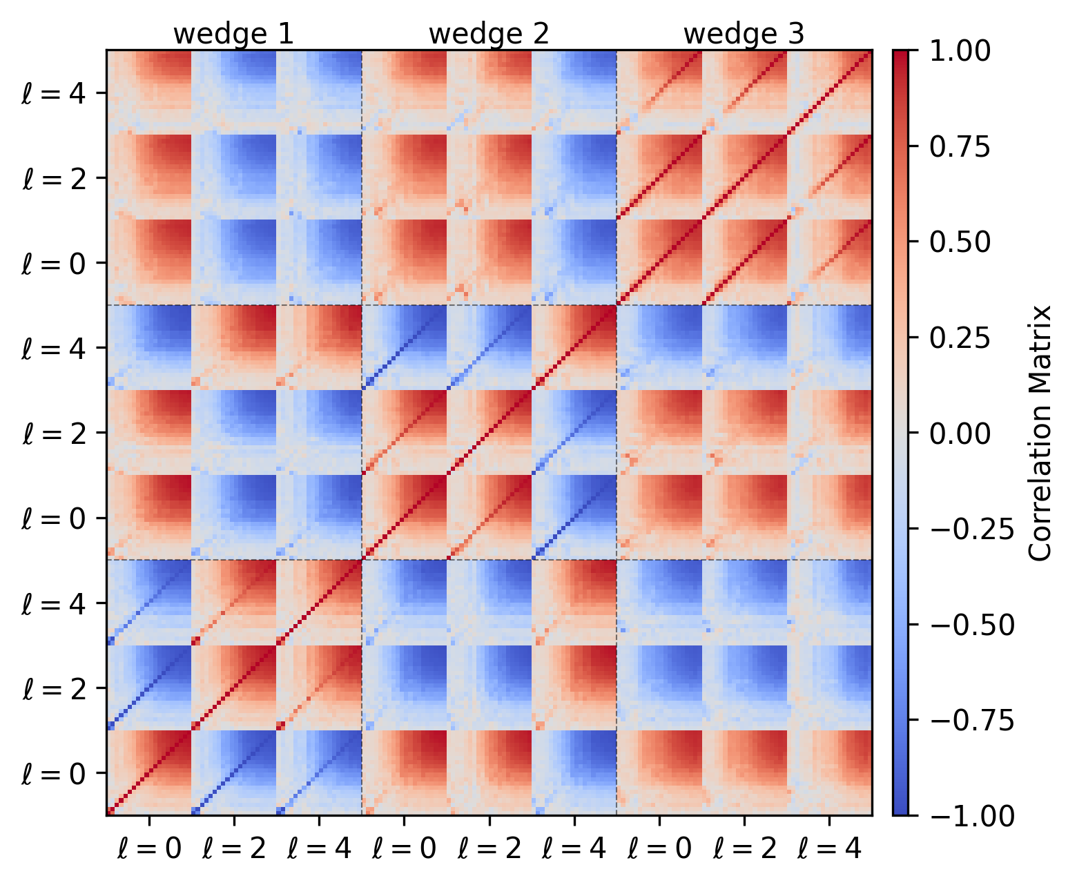
Figure 10: The correlation matrix of the power spectrum multipoles. The $k$ values of the axes are the same as Figure 7 and are omitted for visual clarity.

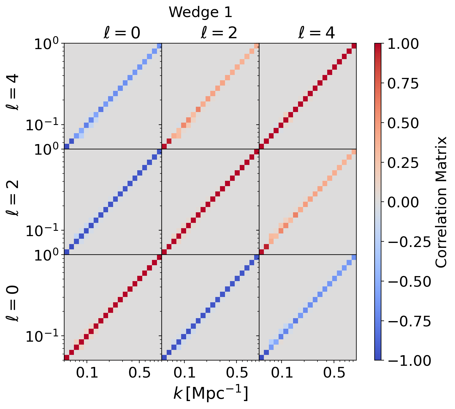
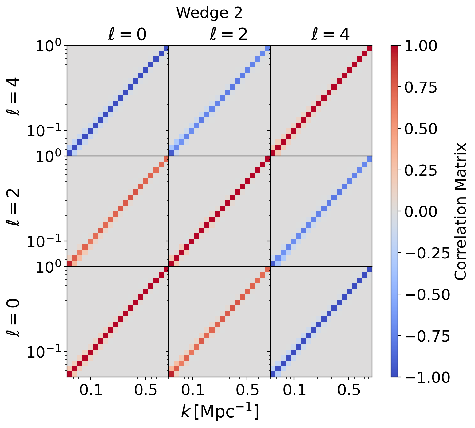
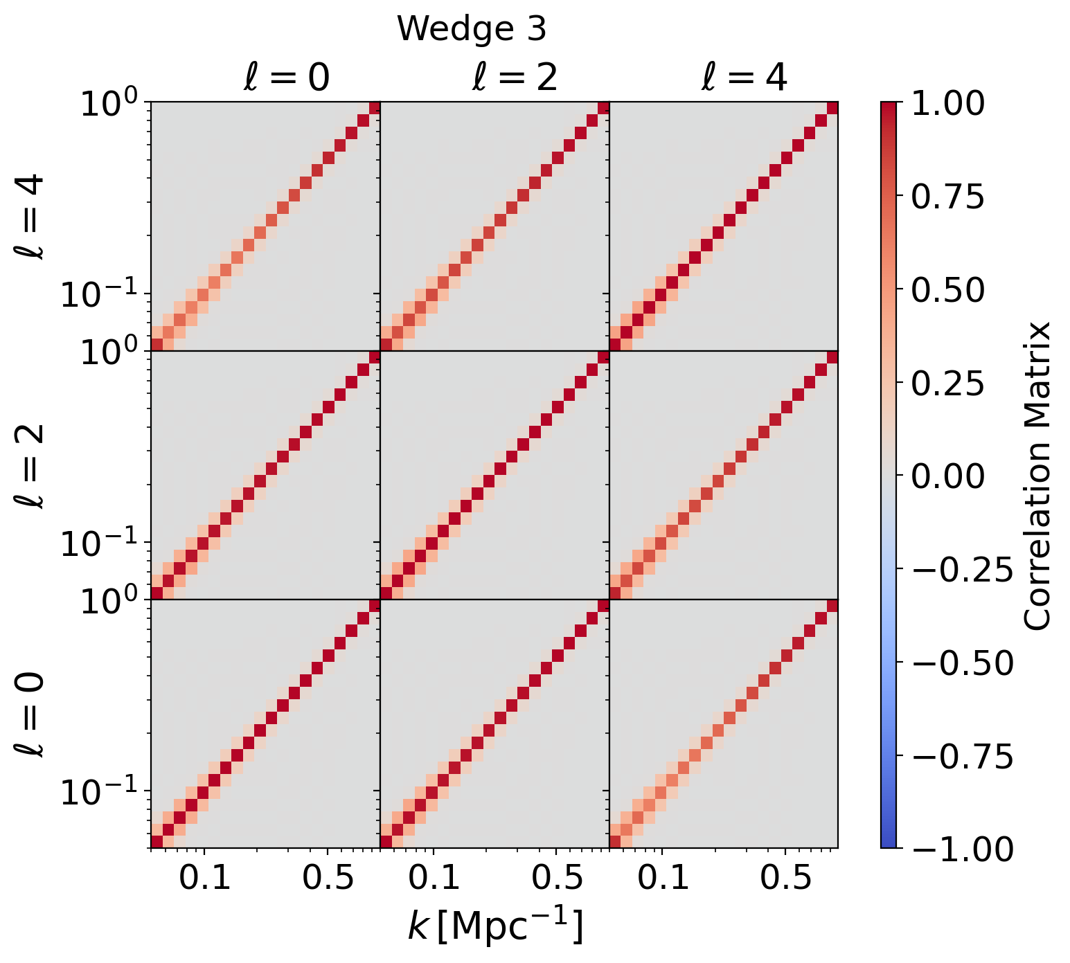
Figure 11: The correlation matrix of noise covariance for different clustering wedges. The amplitude of the noise covariance is shown in Figure 8.

References

- Abdurashidova et al. (2022) Abdurashidova Z., et al., 2022, ApJ, 925, 221
- Adams et al. (2023) Adams N. J., et al., 2023, MNRAS, 518, 4755
- Amiri et al. (2023) Amiri M., et al., 2023, ApJ, 947, 16
- Astropy Collaboration et al. (2018) Astropy Collaboration et al., 2018, AJ, 156, 123
- Austin et al. (2023) Austin D., et al., 2023, ApJ, 952, L7
- Bag et al. (2019) Bag S., Mondal R., Sarkar P., Bharadwaj S., Choudhury T. R., Sahni V., 2019, MNRAS, 485, 2235
- Barkana & Loeb (2001) Barkana R., Loeb A., 2001, Phys. Rep., 349, 125
- Barry et al. (2016) Barry N., Hazelton B., Sullivan I., Morales M. F., Pober J. C., 2016, MNRAS, 461, 3135
- Battye et al. (2004) Battye R. A., Davies R. D., Weller J., 2004, MNRAS, 355, 1339
- Berti et al. (2023) Berti M., Spinelli M., Viel M., 2023, Mon. Not. Roy. Astron. Soc., 521, 3221
- Bosman et al. (2022) Bosman S. E. I., et al., 2022, MNRAS, 514, 55
- Braun et al. (2019) Braun R., Bonaldi A., Bourke T., Keane E., Wagg J., 2019, arXiv e-prints, p. arXiv:1912.12699
- Byrne et al. (2019) Byrne R., et al., 2019, ApJ, 875, 70
- CASA Team et al. (2022) CASA Team et al., 2022, PASP, 134, 114501
- Castellano et al. (2022) Castellano M., et al., 2022, ApJ, 938, L15
- Chang et al. (2008) Chang T.-C., Pen U.-L., Peterson J. B., McDonald P., 2008, Phys. Rev. Lett., 100, 091303
- Chapman & Santos (2019) Chapman E., Santos M. G., 2019, MNRAS, 490, 1255
- Chapman et al. (2012) Chapman E., et al., 2012, MNRAS, 423, 2518
- Chen et al. (2019) Chen Z., Xu Y., Wang Y., Chen X., 2019, ApJ, 885, 23
- Chen et al. (2023a) Chen Z., Wolz L., Battye R., 2023a, MNRAS, 518, 2971
- Chen et al. (2023b) Chen Z., Chapman E., Wolz L., Mazumder A., 2023b, MNRAS, 524, 3724
- Condon & Ransom (2016) Condon J. J., Ransom S. M., 2016, Essential Radio Astronomy, sch - school edition edn. Princeton University Press, http://www.jstor.org/stable/j.ctv5vdcww
- Cooray (2006) Cooray A., 2006, Phys. Rev. Lett., 97, 261301
- Cooray et al. (2008) Cooray A., Li C., Melchiorri A., 2008, Phys. Rev. D, 77, 103506
- Cramér (1999) Cramér H., 1999, Mathematical Methods of Statistics (PMS-9). Princeton University Press, http://www.jstor.org/stable/j.ctt1bpm9r4
- Cunnington et al. (2020) Cunnington S., Pourtsidou A., Soares P. S., Blake C., Bacon D., 2020, Mon. Not. Roy. Astron. Soc., 496, 415
- Cunnington et al. (2023) Cunnington S., et al., 2023, MNRAS, 518, 6262
- Datta et al. (2012) Datta K. K., Mellema G., Mao Y., Iliev I. T., Shapiro P. R., Ahn K., 2012, MNRAS, 424, 1877
- Datta et al. (2014) Datta K. K., Jensen H., Majumdar S., Mellema G., Iliev I. T., Mao Y., Shapiro P. R., Ahn K., 2014, MNRAS, 442, 1491
- Davies et al. (2018) Davies F. B., et al., 2018, ApJ, 864, 142
- DeBoer et al. (2017) DeBoer D. R., et al., 2017, PASP, 129, 045001
- Euclid Collaboration et al. (2020) Euclid Collaboration et al., 2020, A&A, 642, A191
- Finkelstein et al. (2023) Finkelstein S. L., et al., 2023, ApJ, 946, L13
- Furlanetto & Oh (2016) Furlanetto S. R., Oh S. P., 2016, MNRAS, 457, 1813
- Furlanetto et al. (2004) Furlanetto S. R., Zaldarriaga M., Hernquist L., 2004, ApJ, 613, 1
- Furlanetto et al. (2006) Furlanetto S. R., Oh S. P., Briggs F. H., 2006, Phys. Rep., 433, 181
- Gardner et al. (2023) Gardner J. P., et al., 2023, PASP, 135, 068001
- Georgiev et al. (2022) Georgiev I., Mellema G., Giri S. K., Mondal R., 2022, MNRAS, 513, 5109
- Giri & Mellema (2021) Giri S. K., Mellema G., 2021, MNRAS, 505, 1863
- Giri et al. (2018a) Giri S. K., Mellema G., Dixon K. L., Iliev I. T., 2018a, MNRAS, 473, 2949
- Giri et al. (2018b) Giri S. K., Mellema G., Ghara R., 2018b, MNRAS, 479, 5596
- Gnedin & Ostriker (1997) Gnedin N. Y., Ostriker J. P., 1997, ApJ, 486, 581
- Greig & Mesinger (2015) Greig B., Mesinger A., 2015, MNRAS, 449, 4246
- Greig & Mesinger (2018) Greig B., Mesinger A., 2018, MNRAS, 477, 3217
- Greig et al. (2024a) Greig B., Prelogović D., Qin Y., Ting Y.-S., Mesinger A., 2024a, arXiv e-prints, p. arXiv:2403.14060
- Greig et al. (2024b) Greig B., et al., 2024b, arXiv e-prints, p. arXiv:2404.12585
- HERA Collaboration et al. (2023) HERA Collaboration et al., 2023, ApJ, 945, 124
- Hamilton (1997) Hamilton A. J. S., 1997, MNRAS, 289, 285
- Harikane et al. (2023) Harikane Y., et al., 2023, ApJS, 265, 5
- Harris et al. (2020) Harris C. R., et al., 2020, Nature, 585, 357
- Hassan et al. (2016) Hassan S., Davé R., Finlator K., Santos M. G., 2016, MNRAS, 457, 1550
- Haynes et al. (2018) Haynes M. P., et al., 2018, ApJ, 861, 49
- Hellwig et al. (1970) Hellwig H., Vessot R. F. C., Levine M. W., Zitzewitz P. W., Allan D. W., Glaze D. J., 1970, IEEE Transactions on Instrumentation Measurement, 19, 200
- Hunter (2007) Hunter J. D., 2007, Computing in Science & Engineering, 9, 90
- Jensen et al. (2013) Jensen H., et al., 2013, MNRAS, 435, 460
- Jensen et al. (2016) Jensen H., Majumdar S., Mellema G., Lidz A., Iliev I. T., Dixon K. L., 2016, MNRAS, 456, 66
- Kern & Liu (2021) Kern N. S., Liu A., 2021, MNRAS, 501, 1463
- Kern et al. (2020) Kern N. S., et al., 2020, ApJ, 888, 70
- Lewis et al. (2000) Lewis A., Challinor A., Lasenby A., 2000, ApJ, 538, 473
- Liu & Shaw (2020) Liu A., Shaw J. R., 2020, PASP, 132, 062001
- Liu & Tegmark (2011) Liu A., Tegmark M., 2011, Phys. Rev. D, 83, 103006
- Liu et al. (2014) Liu A., Parsons A. R., Trott C. M., 2014, Phys. Rev. D, 90, 023018
- Lynch et al. (2021) Lynch C. R., et al., 2021, Publ. Astron. Soc. Australia, 38, e057
- Madau et al. (1997) Madau P., Meiksin A., Rees M. J., 1997, ApJ, 475, 429
- Majumdar et al. (2018) Majumdar S., Pritchard J. R., Mondal R., Watkinson C. A., Bharadwaj S., Mellema G., 2018, MNRAS, 476, 4007
- Mao et al. (2012) Mao Y., Shapiro P. R., Mellema G., Iliev I. T., Koda J., Ahn K., 2012, MNRAS, 422, 926
- McQuinn et al. (2006) McQuinn M., Zahn O., Zaldarriaga M., Hernquist L., Furlanetto S. R., 2006, ApJ, 653, 815
- Mellema et al. (2013) Mellema G., et al., 2013, Experimental Astronomy, 36, 235
- Mertens et al. (2020) Mertens F. G., et al., 2020, MNRAS, 493, 1662
- Mesinger & Furlanetto (2007) Mesinger A., Furlanetto S., 2007, ApJ, 669, 663
- Mesinger et al. (2011) Mesinger A., Furlanetto S., Cen R., 2011, MNRAS, 411, 955
- Mondal et al. (2017) Mondal R., Bharadwaj S., Majumdar S., 2017, MNRAS, 464, 2992
- Morales & Hewitt (2004) Morales M. F., Hewitt J., 2004, ApJ, 615, 7
- Morales et al. (2012) Morales M. F., Hazelton B., Sullivan I., Beardsley A., 2012, ApJ, 752, 137
- Mort et al. (2010) Mort B. J., Dulwich F., Salvini S., Adami K. Z., Jones M. E., 2010, in 2010 IEEE International Symposium on Phased Array Systems and Technology. pp 690–694, doi:10.1109/ARRAY.2010.5613289
- Murray et al. (2020) Murray S., Greig B., Mesinger A., Muñoz J., Qin Y., Park J., Watkinson C., 2020, The Journal of Open Source Software, 5, 2582
- Offringa et al. (2015) Offringa A. R., et al., 2015, Publ. Astron. Soc. Australia, 32, e008
- Park et al. (2019) Park J., Mesinger A., Greig B., Gillet N., 2019, MNRAS, 484, 933
- Parsons et al. (2012) Parsons A. R., Pober J. C., Aguirre J. E., Carilli C. L., Jacobs D. C., Moore D. F., 2012, ApJ, 756, 165
- Parsons et al. (2014) Parsons A. R., et al., 2014, ApJ, 788, 106
- Paszke et al. (2019) Paszke A., et al., 2019, in Wallach H., Larochelle H., Beygelzimer A., d'Alché-Buc F., Fox E., Garnett R., eds, , Advances in Neural Information Processing Systems 32. Curran Associates, Inc., pp 8024–8035
- Paul et al. (2023) Paul S., Santos M. G., Chen Z., Wolz L., 2023, arXiv e-prints, p. arXiv:2301.11943
- Planck Collaboration et al. (2020) Planck Collaboration et al., 2020, A&A, 641, A6
- Pourtsidou (2023) Pourtsidou A., 2023, MNRAS, 519, 6246
- Prelogović & Mesinger (2024) Prelogović D., Mesinger A., 2024, arXiv e-prints, p. arXiv:2401.12277
- Press & Schechter (1974) Press W. H., Schechter P., 1974, ApJ, 187, 425
- Raghunathan et al. (2023) Raghunathan A., Satish K., Sathyamurthy A., Prabu T., Girish B. S., Srivani K. S., Sethi S. K., 2023, Journal of Astrophysics and Astronomy, 44, 43
- Rao (1992) Rao C. R., 1992, Information and the Accuracy Attainable in the Estimation of Statistical Parameters. Springer New York, New York, NY, pp 235–247, doi:10.1007/978-1-4612-0919-5_16, https://doi.org/10.1007/978-1-4612-0919-5_16
- Raut et al. (2018) Raut D., Choudhury T. R., Ghara R., 2018, MNRAS, 475, 438
- Santini et al. (2023) Santini P., et al., 2023, ApJ, 942, L27
- Santos et al. (2016) Santos M., et al., 2016, in MeerKAT Science: On the Pathway to the SKA. p. 32 (arXiv:1709.06099), doi:10.22323/1.277.0032
- Schaeffer et al. (2024) Schaeffer T., Giri S. K., Schneider A., 2024, arXiv e-prints, p. arXiv:2404.08042
- Scoccimarro (2015) Scoccimarro R., 2015, Phys. Rev. D, 92, 083532
- Shaw et al. (2020) Shaw A. K., Bharadwaj S., Mondal R., 2020, MNRAS, 498, 1480
- Sheth & Tormen (1999) Sheth R. K., Tormen G., 1999, MNRAS, 308, 119
- Shimabukuro et al. (2015) Shimabukuro H., Yoshiura S., Takahashi K., Yokoyama S., Ichiki K., 2015, MNRAS, 451, 467
- Shimabukuro et al. (2017) Shimabukuro H., Yoshiura S., Takahashi K., Yokoyama S., Ichiki K., 2017, MNRAS, 468, 1542
- Smirnov (2011) Smirnov O. M., 2011, A&A, 527, A106
- Soares et al. (2021) Soares P. S., Cunnington S., Pourtsidou A., Blake C., 2021, Mon. Not. Roy. Astron. Soc., 502, 2549
- Sobacchi & Mesinger (2014) Sobacchi E., Mesinger A., 2014, MNRAS, 440, 1662
- Sokolowski et al. (2015) Sokolowski M., Wayth R. B., Lewis M., 2015, in 2015 IEEE Global Electromagnetic Compatibility Conference (GEMCCON). pp 1–6, doi:10.1109/GEMCCON.2015.7386856
- Tegmark (1997) Tegmark M., 1997, Phys. Rev. D, 55, 5895
- Tegmark & de Oliveira-Costa (2001) Tegmark M., de Oliveira-Costa A., 2001, Phys. Rev. D, 64, 063001
- Tegmark et al. (1998) Tegmark M., Hamilton A. J. S., Strauss M. A., Vogeley M. S., Szalay A. S., 1998, ApJ, 499, 555
- Thyagarajan et al. (2015) Thyagarajan N., et al., 2015, ApJ, 804, 14
- Tingay et al. (2013) Tingay S. J., et al., 2013, Publ. Astron. Soc. Australia, 30, e007
- Trott et al. (2020) Trott C. M., et al., 2020, MNRAS, 493, 4711
- Virtanen et al. (2020) Virtanen P., et al., 2020, Nature Methods, 17, 261
- Wagoner et al. (1967) Wagoner R. V., Fowler W. A., Hoyle F., 1967, ApJ, 148, 3
- Wang et al. (2021) Wang J., et al., 2021, MNRAS, 505, 3698
- Watkinson et al. (2022) Watkinson C. A., Greig B., Mesinger A., 2022, MNRAS, 510, 3838
- Wilensky et al. (2019) Wilensky M. J., Morales M. F., Hazelton B. J., Barry N., Byrne R., Roy S., 2019, PASP, 131, 114507
- Wilensky et al. (2022) Wilensky M. J., Hazelton B. J., Morales M. F., 2022, MNRAS, 510, 5023
- Wolz et al. (2022) Wolz L., et al., 2022, MNRAS, 510, 3495
- Yatawatta et al. (2013) Yatawatta S., et al., 2013, A&A, 550, A136
- Yoshiura et al. (2017) Yoshiura S., Shimabukuro H., Takahashi K., Matsubara T., 2017, MNRAS, 465, 394
- Yoshiura et al. (2021) Yoshiura S., et al., 2021, MNRAS, 505, 4775
- Zhang et al. (2023) Zhang C.-P., et al., 2023, arXiv e-prints, p. arXiv:2312.06097
- Zhao et al. (2022) Zhao X., Mao Y., Cheng C., Wandelt B. D., 2022, ApJ, 926, 151