Planning with Probabilistic Opacity and Transparency: A Computational Model of Opaque/Transparent Observations

Abstract

Qualitative opacity of a secret is a security property, which means that a system trajectory satisfying the secret is observation-equivalent to a trajectory violating the secret. In this paper, we study how to synthesize a control policy that maximizes the probability of a secret being made opaque against an eavesdropping attacker/observer, while subject to other task performance constraints. In contrast to existing belief-based approach for opacity-enforcement, we develop an approach that uses the observation function, the secret, and the model of the dynamical systems to construct a so-called opaque-observations automaton which accepts the exact set of observations that enforce opacity. Leveraging this opaque-observations automaton, we can reduce the optimal planning in Markov decision processes(MDPs) for maximizing probabilistic opacity or its dual notion, transparency, subject to task constraints into a constrained planning problem over an augmented-state MDP. Finally, we illustrate the effectiveness of the developed methods in robot motion planning problems with opacity or transparency requirements.

I Introduction

Opacity is a security and privacy property that evaluates whether an observer (intruder) can deduce a system’s secret by monitoring its behavior. A system is opaque if its secret behavior or private information is made uncertain to an adversarial intruder. Initially introduced for cryptographic protocols by Mazaré [12], opacity has since then been explored with various notions depending on the nature of the secret. For instance, state-based opacity ensures that the observer cannot discern if a secret state has been visited, language-based opacity enforces that the observer cannot discern if the trajectory is in a set of secret trajectories[5, 4, 14, 17, 8, 2].

To set the context, consider a scenario involving an autonomous robot (Player 1 or P1) tasked with routine monitoring in a power plant. A sensor network is deployed for daily activity monitoring but can be vulnerable to eavesdropping attacks. Should there be an unauthorized Player 2 (P2) observing the sensor network, P1 must make P2 uncertain if a sequence of waypoints has been visited to enforce location security. Now, the planning question is how can P1 ensure maximal opacity to P2, while fulfilling the routine task beyond a specific threshold?

In this study, we explore language-based opacity and its dual notion, transparency, in stochastic systems with two players, where one player has imperfect observations. Quantitative opacity quantifies the security level of a system [3]. In competitive settings, achieving maximum probabilistic opacity under task constraints is crucial, while in cooperative scenarios like human-robot interactions, maximizing probabilistic transparency is essential.

The classical approach for opacity enforcement is to construct a belief-based planning problem (see Related Work) where P1 tracks P2’s belief state regarding the current or past state. However, this approach is computational expensive.

Instead, we present an approach to construct a computational model of opaque observations, which are observations obtained by state trajectories that enforce opacity. We use a Finite State Transducer (FST) to encode the observation function of state trajectories and then the synchronization product between the FST and secret language, expressed as a Deterministic Finite Automaton (DFA), to construct another DFA accepting the set of opaque observations. A product between the Markov decision process (MDP), task DFA, and the opaque-observations DFA is then computed. We show that the maximally opaque (maximally transparent) control policy under the task performance constraints can be solved as a constrained planning problem in this product.

I-A Related Work

In the supervisory control of discrete event systems (DES), researchers have developed opacity-enforcing controllers by modelling the control systems as a DFA in the presence of a passive observer [13, 14, 24]. Different approaches have been proposed to either synthesize [6, 20, 21] or verify opacity [9, 15, 19] in deterministic systems. Saboori et al. [16] synthesized a supervisor to enforce qualitative opacity by restricting system behaviors. Cassez et al. [6] suggests using a dynamic mask to filter unobservable events, verifying opacity through solving a 2-player safety game. In [21], Xie et al. proposed a nondeterministic supervisor to prevent the observer, aware of the supervisor’s nondeterminism, from determining the secret. Besides enforcing opacity, sensor attack strategies to compromise opacity has been investigated in [22], where they proposed an information structure that records state estimates for both the supervisor and attacker. In game-theoretic approaches to opacity enforcement, Maubert et al. [11] introduced a game where a player with perfect observations aims to enforce current state opacity against another player with imperfect observations. In our previous work [18] we explored qualitative opacity enforcement in a stochastic environment with both the players having partial observation. These works primarily address qualitative opacity, whereas our research examines the probabilistic notions of opacity and transparency.

In stochastic DESs, several studies delve into quantifying opacity. Saboori et al. [17] introduced notions of current state opacity for probabilistic finite automata, along with verification algorithms to verify if the system is probabilistically opaque for a given threshold. Yin et al. [23] extended this to the notions of infinite and K-step opacity. Keroglou et al. [8] explored model-based opacity, where the defender conceals the system model using a hidden Markov model. Bérard et al. [2] extended language-based opacity to $\omega$-regular properties on MDP. Bérard et al. define the notions of symmetrical opacity, and define probabilistic disclosures. They showed that the quantitative questions relating to opacity become decidable for the class of $\omega$-regular secrets. Liu et al. [10] studied approximate opacity in continuous stochastic control systems, developing a verification method for general continuous-state MDPs with finite abstractions.

Our proposed approach considers probabilistic opacity/transparency-enforcement in MDPs, distinguishing it from qualitative approaches. In existing stochastic methods, verification commonly involves tracking current state estimates or maintaining a belief state for opacity enforcement. In our method, we instead study an FST-based computational model of opaque observations to directly encode state trajectories, allowing us to construct another DFA that precisely accepts the set of opaque observations to enforce opacity/transparency. Our proposed computational model has the potential for extension to scenarios involving active attackers, without the need for tracking the belief of state estimates for the agents (a direction we leave for future work).

Organization

In Section II, we introduce preliminaries, and frame the problem. Section III presents our computational model. In Section IV, we use the computational model to solve an optimal planning problem. Section V illustrates the planning problem’s application in a gridworld scenario. Finally, we conclude in Section VI.

II Preliminaries and Problem Formulation

Notations

Let $\Sigma$ be a finite set of symbols, called the alphabet. We denote a set of all $\omega$-regular words as $\Sigma^{\omega}$ obtained by concatenating the elements in $\Sigma$ infinitely many times. A sequence of symbols $w=\sigma_{0}\sigma_{1}\cdots\sigma_{n}$ with $\sigma_{i}\in\Sigma$ for any $0\leq i\leq n$, is a finite word. The set $\Sigma^{*}$ is the set of all finite words that can be generated with $\Sigma$. The length of a word is denoted by $|w|$. For a word $w=uv$, $u$ is a prefix of $v$ for $u\in\Sigma^{\ast}$ and $v\in\Sigma^{\omega}$. Let $\mathbf{R}$ denote the set of real numbers. Given a finite set $Z$, the set of probability distributions over $Z$ is represented as $\mathcal{D}(Z)$. Given $d\in\mathcal{D}(Z)$, the support of $d$ is $\mathsf{Supp}(d)=\{z\in Z\mid d(z)>0\}$.

II-A Markov decision process

We consider the interaction of P1 with a stochastic environment, monitored by P2 with partial observations, modeled as a terminating MDP (without the reward function).

Definition 1.

A probabilistic transition system (i.e. , an MDP without the reward function) is a tuple

$$M=(S,A,P,\mu_{0},s_{\top},s_{\bot},\mathcal{AP},O,L)$$

where $S$ is a finite set of states, $A$ is a finite set of actions. $s_{\top}\in S$ is the initiating state, which is a unique start state. $s_{\bot}\in S$ is the terminating state, which is a unique sink state. The set $A$ is the action set, which includes a special initiating action and a terminating action $a_{\top}$ and $a_{\bot}$ respectively. $a_{\top}$ is only enabled in $s_{\top}$, while $a_{\bot}$ is enabled for any $s\in S\setminus\{s_{\top},s_{\bot}\}$. $P:S\times A\rightarrow\mathcal{D}(S)$ is a probabilistic transition function, with $P(s^{\prime}|s,a)$ representing the probability of reaching state $s^{\prime}$ given action $a$ at state $s$. $\mu_{0}$ is the initial distribution on states $S\setminus\{s_{\top}\}$ such that $\mu_{0}(s)$ represents the probability of $s$ being the initial state. For $s_{\top}\in S$, $P(s_{\top},a_{\top},s)=\mu_{0}(s)$. That is, if P1 selects the initiating action $a_{\top}$, then an initial state is reached surely. For any $s\in S\setminus\{s_{\top},s_{\bot}\}$, $P(s,a_{\bot},s_{\bot})=1$. That is, if P1 selects the terminating action $a_{\bot}$, then a terminating state $s_{\bot}$ is reached surely. Finally, for any $a\in A\setminus\{a_{\top},a_{\bot}\}$, $P(s_{\bot},a,s_{\bot})=1$, i.e. , all allowed actions form a self-loop. $\mathcal{AP}$ is a set of atomic propositions, $L:S\rightarrow 2^{\mathcal{AP}}$ is the labeling function that maps a state to a set of atomic propositions that evaluate true at that state. The initiating state is labeled with a “starting” symbol, $\rtimes$, i.e. , $L(s_{\top})=\rtimes$. The terminating state is labeled the “ending” symbol $\ltimes$, i.e. , $L(s_{\bot})=\ltimes$. $O\subseteq 2^{S}$ is the set of all finite observables.

A finite play $\rho=s_{\top}a_{\top}s_{0}a_{0}s_{1}\ldots s_{n}a_{\bot}s_{\bot}$ is a sequence of interleaving states and player’s actions, where for all $i\geq 0$, $P(s_{i+1}\mid s_{i},a_{i})>0$. Let $\mathsf{Plays}(M)\subseteq(S\times A)^{\ast}S$ be the set of finite plays that can be generated from the game $M$. The labeling of a finite play, denoted by $L(\rho)$, is defined as $L(\rho)=\rtimes L(s_{0})L(s_{1})\ldots L(s_{n})\ltimes$ i.e. , the labeling function omits the actions from the play and applies to states only.

A randomized, finite-memory strategy is a function $\pi:\mathsf{Plays}(M)\rightarrow\mathcal{D}(A)$ mapping a play to a distribution over actions. A randomized, Markov strategy is a function $\pi:S\rightarrow\mathcal{D}(A)$ mapping the current state to a distribution over actions. The stochastic process generated by applying a policy $\pi$ to the MDP $M$ is denoted as $M^{\pi}$, with transition dynamics $P^{\pi}(s\mid s_{\top})=\mu_{0}(s)$ for the initiating state and $P^{\pi}(s^{\prime}\mid s)=\sum_{a\in A}P(s,a,s^{\prime})\cdot\pi(a\mid s)$ for all $s\in S\setminus\{s_{\top}\}$.

Information structure

We assume that 1. P1 has perfect observation of states and actions. 2. P2 has partial observation of states and no observation of P1’s actions.

Definition 2 (Transition-Observation function).

The transition-observation function of P2 is $\mathsf{Obs}:S\times A\times S\rightarrow O$ mapping a transition $(s,a,s^{\prime})$ to an observation $o\in O$. The observation function of P2 is extended to plays in $M$ as $\mathsf{Obs}:\mathsf{Plays}(M)\rightarrow O^{\ast}$ such that for any play $\rho=\rho_{1}\cdot s_{n}a_{n}s_{n+1}$, $\mathsf{Obs}(\rho)=\mathsf{Obs}(\rho_{1})\cdot\mathsf{Obs}(s_{n}a_{n}s_{n+1})$ which is the observation of the prefix $\rho_{1}$ concatenated with the observation of the last transition. Two plays $\rho_{1},\rho_{2}$ are observation-equivalent iff $\mathsf{Obs}(\rho_{1})=\mathsf{Obs}(\rho_{2})$.

The inverse observation function of P2 $\mathsf{Obs}^{-1}:\mathsf{Obs}(M)\rightarrow 2^{\mathsf{Plays}(M)}$ maps each $\eta\in\mathsf{Obs}(M)$ to the set $\mathsf{Obs}^{-1}(\eta)=\{\rho\in\mathsf{Plays}(M)\mid\mathsf{Obs}(\rho)=\eta\}$. Given a play $\rho\in\mathsf{Plays}(M)$, we denote the set of plays that are observation-equivalent to $\rho$ in P2’s perspective by $[\rho]_{2}$.

Objective and secret in temporal logic In the game arena, P1 aims to achieve a temporal objective $\psi$ specified by a Linear Temporal Logic over Finite Traces (LTL_f) formula, while P2 observes P1. P1 also holds a secret LTL_f formula $\varphi$ with the goal of concealing whether $\varphi$ is satisfied or not from P2. The two formulas $\psi$ and $\varphi$ may be different.

The syntax of the LTL_f formula is given as follows.

Definition 3 (LTL_f [7]).

An (LTL_f) formula over $\mathcal{AP}$ is defined inductively as follows:

$$\varphi:=p\mid\neg\varphi\mid\varphi_{1}\land\varphi_{2}\mid\varphi_{1}\lor\varphi_{2}\mid\bigcirc\,\varphi\mid\varphi_{1}\mbox{$\,{\sf U}\,$}\varphi_{2}\mid\Diamond\,\varphi\mid\Box\,\varphi,$$

where $p\in\mathcal{AP}$; $\neg$, $\land$ and $\lor$ are the Boolean operators negation, conjunction and disjunction, respectively; and $\bigcirc\,$, $\,{\sf U}\,$, $\Diamond\,$ and $\Box\,$ denote the temporal modal operators for next, until, eventually and always, respectively.

The operator $\bigcirc\,\varphi$ specifies that formula $\varphi$ holds at the next time instant. $\varphi_{1}\mbox{$\,{\sf U}\,$}\varphi_{2}$ denotes that there exists a future time instant at which $\varphi_{2}$ holds, and that $\varphi_{1}$ holds at all time instants up to and including that future instant. The formula $\Diamond\,\varphi$ specifies that $\varphi$ holds at some future instant, and $\Box\,\varphi$ specifies that $\varphi$ holds at all current and future time instants. See [7] for detailed semantics of LTL_f.

For any LTL_f formula $\varphi$ over $AP$, a set of words $\mathsf{Words}(\varphi)=\{w\subseteq(2^{AP})^{*}\mid w\models\varphi\}$ that satisfy the formula is associated.

Definition 4 (DFA).

A DFA is a tuple $\mathcal{A}=(Q,\Sigma,\delta,{\iota},F)$ with a finite set of states $Q$, a finite alphabet $\Sigma$, a deterministic transition function $\delta:Q\times\Sigma\rightarrow Q$, extended recursively as $\delta(q,\sigma u)=\delta(\delta(q,\sigma),u)$ for $\sigma\in\Sigma,u\in\Sigma^{\ast}$. ${\iota}$ is the initial state, and $F\subseteq Q$ is a set of accepting states.

A Nondeterministic Finite Automaton (NFA) is defined similarly to a DFA, with a nondeterministic transition function $\delta:Q\times\Sigma\rightarrow 2^{Q}$, where for every $q\in Q$ and $\sigma\in\Sigma$, transition occurs to a set of states $X\in 2^{Q}$.

Using the method of De Giacomo and Vardi [7], we convert the LTL_f formulae into DFA that accepts $\mathsf{Words}(\varphi)$ with $\Sigma=2^{\mathcal{AP}}$. We have the DFA accepting all the words satisfying the secret $\varphi$ as $\mathcal{A}_{s}=(Q_{s},2^{\mathcal{AP}},\delta_{s},{\iota}_{s},F_{s})$, and the DFA accepting all words satisfying the task specification $\psi$ as $\mathcal{A}$. Both DFAs are considered to be complete .

II-B Probabilistic opacity and transparency

We introduce the definition of symmetric opacity as in [3].

Definition 5 (Symmetrical Opacity).

An LTL_f formula $\varphi$ is opaque to P2 with respect to a play $\rho\in\mathsf{Plays}(M)$ iff either of the following cases hold: 1. $L(\rho)\models\varphi$; and there exists at least one observation-equivalent play $\rho^{\prime}\in[\rho]_{2}$ with $L(\rho^{\prime})\not\models\varphi$; or 2. $L(\rho)\not\models\varphi$; and there exists at least one observation-equivalent play $\rho^{\prime}\in[\rho]_{2}$ with $L(\rho)\models\varphi$.

We now define transparency as a dual property of opacity.

Definition 6 (Symmetrical Transparency).

An LTL_f formula $\varphi$ is transparent to P2 with respect to a play $\rho\in\mathsf{Plays}(M)$ iff either of the following cases hold: 1. $L(\rho)\models\varphi$; and for any observation-equivalent play $\rho^{\prime}\in[\rho]_{2}$, $L(\rho^{\prime})\models\varphi$, or 2. $L(\rho)\not\models\varphi$; and for any observation-equivalent play $\rho^{\prime}\in[\rho]_{2}$ with $L(\rho)\not\models\varphi$.

We define the set of opaque and non-opaque runs for the secret $\varphi$ and observation function $\mathsf{Obs}$ as follows.

• The set of opaque runs is as given below.

  $$\mathcal{S}_{H}=\{\rho\in\mathsf{Plays}(M)\mid\exists\rho^{\prime}\in[\rho]_{2},(L(\rho)\not\models\varphi\land\\ L(\rho^{\prime})\models\varphi)\lor(L(\rho)\models\varphi\land L(\rho^{\prime})\not\models\varphi)\}$$ (1)

• The set of transparent runs is

  $$\mathcal{S}_{T}=\{\rho\in\mathsf{Plays}(M)\mid\forall\rho^{\prime}\in[\rho]_{2},\\ (L(\rho)\models\varphi\implies L(\rho^{\prime})\models\varphi)\\ \lor(L(\rho)\not\models\varphi\implies L(\rho^{\prime})\not\models\varphi)\}$$ (2)

It is easy to see $\mathcal{S}_{T}\cap\mathcal{S}_{H}=\emptyset$.

Lemma 1.

$\mathcal{S}_{H}\cup\mathcal{S}_{T}=\mathsf{Plays}(M)$.

The proof follows from the definition and thus is omitted.

The following definition of quantitative opacity has been introduced in [2] for probabilistic systems.

Definition 7 (Probabilistic opacity and transparency).

Given the MDP $M$, observation function $\mathsf{Obs}$, the secret $\varphi$ and policy $\pi$, the probabilistic opacity of $\varphi$ in the stochastic process $M^{\pi}$ is

$$PH(\varphi;M^{\pi},\mathsf{Obs})=\Pr(\mathcal{S}_{H};M^{\pi})$$

where $\Pr(\mathcal{S}_{H};M^{\pi})$ denotes the probability of an opaque run given $M^{\pi}$. The probabilistic transparency of $\varphi$ in $M^{\pi}$ is

$$PT(\varphi;M^{\pi},\mathsf{Obs})=\Pr(\mathcal{S}_{T};M^{\pi})$$

We also define the set of runs that satisfy the task specification as given below.

$$\mathcal{S}_{\psi}=\{\rho\in\mathsf{Plays}(M)\mid L(\rho)\models\psi\}$$ (3)

Problem 1.

Given the MDP $M$, secret $\varphi$, task $\psi$ and the observation function $\mathsf{Obs}$, compute a strategy $\pi^{\ast}$ for P1 that maximizes the probabilistic opacity of $\varphi$ while ensuring that the probability of satisfying the task $\psi$ is greater than $\epsilon$. Formally,

$$\max PH(\varphi;M^{\pi},\mathsf{Obs})$$ (4)

$$\textrm{s.t.}\Pr(\mathcal{S}_{\psi};M^{\pi})\geq\epsilon.$$

By replacing the maximization with minimization, and Lemma 1, the solution of the optimization problem is a policy that maximizes the probabilistic transparency of $\varphi$ under a task performance constraint.

To illustrate our definitions, we introduce a running example.

Figure 1: MDP for the illustrative example. The colored boxes represent the observation partition of the state space.

Example 1 (Part I).

Consider the MDP in Fig.1 with $7$ states, $s_{1}$ through $s_{7}$ ($s_{1}$ as the initial state i.e. , $\mu_{0}(s_{1})=1$). Here, $s_{4}$ is a sink, and edges are labeled with actions and transition probabilities. The transition-observation of a transition to P2, $\mathsf{Obs}(s,a,s^{\prime})$, is a set of states that are observation equivalent to $s^{\prime}$ (actions are not observable). The MDP has observation-equivalent states sets $\{s_{1}\}$, $\{s_{2},s_{3}\}$, $\{s_{4}\}$, $\{s_{5},s_{6}\}$ and $\{s_{7}\}$. P1’s task is to eventually reach $s_{4}$ ($\psi=\Diamond\,s_{4}$), and secret formula is satisfied if P1 reaches the state $s_{6}$, ($\varphi=\Diamond\,s_{6}$). P1 must compute a strategy for maximal probabilistic opacity of $\varphi$ while ensuring to satisfy $\psi$ with a probability $\geq\epsilon$. We can also consider the planning problem where P1 is to maximize the probabilistic transparency with respect to $\varphi$ under the task performance constraint.

III Main results

In this section, we present a computational model to obtain the opaque observations of P2. Using this computational model, we formulate constrained MDPs to solve Problem 1.

III-A A computational model for opaque observations

To solve Problem 1, we need to construct the set $\mathcal{S}_{H}$ of opaque runs, which is measurable. However, the set of possible runs in $M$ can be large or infinite, such an enumeration procedure cannot terminate and therefore we cannot construct $\mathcal{S}_{H}$ for planning purpose. We present a method to construct a DFA that accepts the set of opaque observations.

Definition 8 (Opaque observations).

Given the secret $\varphi$, an observation $\rho_{o}\in O^{\ast}$ is opaque iff there is an opaque run $\rho\in\mathcal{S}_{H}$ and $\rho_{o}=\mathsf{Obs}(\rho)$. The set of opaque observations is $\mathsf{OpqObs}$.

First, it is seen that the observation function $\mathsf{Obs}:\mathsf{Plays}(M)\rightarrow O^{\ast}$ can be expressed as an FST whose input strings are $\mathsf{Plays}(M)$ and output strings are the observations of $\mathsf{Plays}(M)$.

Definition 9 (Finite-state transducer representation for the observation function).

The FST encoding of the observation function $\mathsf{Obs}:\mathsf{Plays}(M)\rightarrow O^{\ast}$ is a tuple

$$\mathcal{A}_{o}=\langle S,\Sigma_{I},\Sigma_{O},T_{o}\rangle$$

where

• $S$ is the finite set of states of the MDP.

• $\Sigma_{I}=S\times A\times S$ is the set of input symbols, which are the transitions in the MDP.

• $\Sigma_{O}=O\cup\{\rtimes,\ltimes\}$ is the set of output symbols, which are the observations in the MDP and two symbols $\rtimes$ and $\ltimes$ marking the beginning and ending of a word.

• $T_{o}:S\times\Sigma_{I}\rightarrow S\times\Sigma_{O}$ is a deterministic transition function that maps a given pair of state and input to a next state and an output. The transition function is constructed as follows:

  • if $s_{\top}\in S$ is the initiating state, the input $(s_{\top},a_{\top},s)$ is enabled if $\mu_{0}(s)>0$ in the MDP $M$, then

    $$T_{o}(s_{\top},(s_{\top},a_{\top},s))=(s,\rtimes),$$

  • if $s\in S$, then the input $(s,a,s^{\prime})$ is enabled if $P(s,a,s^{\prime})>0$ in the MDP $M$,

    $$T_{o}(s,(s,a,s^{\prime}))=(s^{\prime},o),$$

    where $o=\mathsf{Obs}(s,a,s^{\prime})$.

  • for any state $s\in S$, if $a_{\bot}$ action is enabled, then

    $$T_{o}(s,(s,a_{\bot},s_{\bot}))=(s_{\bot},\ltimes).$$

A transition from state $t$ to $t^{\prime}$ given input $\sigma\in\Sigma_{I}$ and output $o\in\Sigma_{o}$ is also denoted $t\xrightarrow[o]{\sigma}t^{\prime}$. Given a sequence of inputs, also called input word $w=\sigma_{0}\sigma_{1}\ldots\sigma_{n}$, the transducer generates a sequence of transitions, or a run $\rho=t_{0}\xrightarrow[o_{0}]{\sigma_{0}}t_{1}\xrightarrow[o_{1}]{\sigma_{1}}t_{2}\ldots\xrightarrow[o_{n-1}]{\sigma_{n-1}}t_{n}$ with the output uniquely determined as $w_{o}=o_{0}o_{1}\ldots o_{n}$.

By construction, it is noted that for any play $\rho=s_{\top}a_{\top}s_{0}\ldots s_{n}a_{\bot}s_{\bot}$, the corresponding input to the FST is

$$\mathsf{In}(\rho)=(s_{\top},a_{\top},s_{0})(s_{0},a_{0},s_{1})(s_{1},a_{1},s_{2})\ldots\\ (s_{n-1},a_{n-1},s_{n})(s_{n},a_{\bot},s_{\bot}).$$

The output is

$$\mathsf{Out}(\rho)=\rtimes\mathsf{Obs}(s_{0},a_{0},s_{1})\mathsf{Obs}(s_{1},a_{1},s_{2})\ldots\\ \mathsf{Obs}(s_{n-1},a_{n-1},s_{n})\ltimes.$$

The corresponding run is $\mathsf{Run}(\rho)=s_{\top}s_{0}s_{1}s_{2}\ldots s_{n}s_{\bot}.$

Example 2 (Part II).

Continuing the Example 1, a fraction of FST encoding of the observation function is shown in Fig. 2. Each of the states in the transducer represent the states in the MDP shown in Fig. 1 along with initiating ($s_{\top}$) and terminating ($s_{\bot}$) states. Transitions are labeled with input and output symbols. For instance, the transition from $s_{1}$ to $s_{2}$ is labeled $(s_{1},a,s_{2})$ as input and $[s_{2},s_{3}]$ as output symbols. Each state also has a transition to the terminating state $s_{\bot}$.

Figure 2: A fragment of FST encoding the observation function.

The next step is to compute a product between the FST of the observation function and the DFA accepting the secret.

Definition 10 (Product FST).

Given the FST representation of the observation function $\mathcal{A}_{o}$, and the secret DFA $\mathcal{A}_{s}$, the product of the FST and DFA is a tuple,

$$\mathcal{A}_{H}=\langle Q_{h},\Sigma_{I},\Sigma_{O},T_{h},{\iota}_{h},F_{h}\rangle$$

• $Q_{h}=S\times Q_{s}$ is the set of states.

• ${\iota}_{h}=(s_{\top},{\iota}_{s})$ is the initial state.

• $T_{h}:Q_{h}\times\Sigma_{I}\rightarrow Q_{h}\times\Sigma_{O}$ is the transition function and is defined as follows. We consider the following cases: For $\sigma\in S\times A\times S$, if $s\xrightarrow[o]{\sigma}s^{\prime}$ in $\mathcal{A}_{o}$ and $q\xrightarrow[]{a}q^{\prime}$ in $\mathcal{A}_{s}$, then,

  1. For $\sigma=(s_{\top},a_{\top},s)$, and $s_{\top}\xrightarrow[\rtimes]{\sigma}s$, let

     $$(s_{\top},{\iota}_{s})\xrightarrow[\rtimes]{\sigma}(s,q)$$

     where $q=\delta({\iota}_{s},L(s))$.

  2. For $\sigma=(s,a_{\bot},s_{\bot})$, and $s\xrightarrow[\ltimes]{\sigma}s_{\bot}$, let

     $$(s,q)\xrightarrow[\ltimes]{\sigma}(s_{\bot},q).$$

  3. For any other $\sigma$, let

     $$(s,q)\xrightarrow[o]{\sigma}(s^{\prime},q^{\prime})\text{ if and only if }\delta_{s}(q,L(s^{\prime}))=q^{\prime}.$$

  4. Any state $(s,q)$ where $s=s_{\bot}$ is a sink state.

• $F_{h}=\{(s_{\bot},q)\mid q\in F_{s}\}$ is a set of accepting states.

From the above construction, we establish a mapping $\mathfrak{R}:\mathsf{Plays}(M)\rightarrow\mathsf{Run}(\mathcal{A}_{H})$ between plays in MDP $M$ and runs in the product of the FST and DFA $\mathcal{A}_{H}$ as follows: For a play $\rho=s_{\top}a_{\top}s_{0}\ldots s_{n}a_{\bot}s_{\bot}\in\mathsf{Plays}(M)$, there is a run (i.e. , a state sequence augmented with automata states) $\hat{\rho}$ such that $\hat{\rho}=(s_{\top},{\iota}_{s})(s_{0},q_{0})\ldots(s_{n},q_{n})(s_{\bot},q_{n})$ where $q_{i}=\delta(q_{i-1},L(s_{i}))$ for $i\geq 1$ and $q_{0}=\delta({\iota}_{s},L(s_{0}))$.

Lemma 2.

A run $\rho\in\mathsf{Plays}(M)$ is such that $L(\rho)\models\varphi$ iff $\mathfrak{R}(\rho)$ ends in $(s_{\bot},q)$ where $q\in F_{s}$.

Proof.

By construction, consider a run $\rho=s_{\top}a_{\top}\ldots a_{\bot}s_{\bot}\\ \in\mathsf{Plays}(M)$, if $\mathfrak{R}(\rho)$ ends in $(s_{\bot},q)$ with $q\in F_{s}$, then $L(s_{\top}s_{0}\ldots s_{n}s_{\bot})$ is accepted by $\mathcal{A}_{s}$. Thus, $L(\rho)\models\varphi$. ∎

We denote the last/final state of $\mathfrak{R}(\rho)$ as $\mathsf{Last}(\rho)$. We then compute two NFAs from the product transducer.

Definition 11.

Given the product FST $\mathcal{A}_{H}=\langle Q_{h},\Sigma_{I},\Sigma_{O},T_{h},{\iota}_{h},F_{h}\rangle$, the output language accepted by $\mathcal{A}_{H}$ is obtained as the set $L_{O}(\mathcal{A}_{H})=\{\mathsf{Out}(\rho)\mid\rho\in\Sigma_{I}^{\ast},\mathsf{Last}(\rho)\in\{s_{\bot}\}\times F_{s}\}$.

The NFA accepting $L_{O}(\mathcal{A}_{H})$ is obtained from $\mathcal{A}_{H}$ by removing the input symbols and use the output symbols on each transition as the input symbol.

Lemma 3.

For any $\rho\in\mathsf{Plays}(M)$, if $\rho\models\varphi$, $\mathsf{Out}(\rho)\in L_{O}(\mathcal{A}_{H})$ and if $\rho\not\models\varphi$, $\mathsf{Out}(\rho)\notin L_{O}(\mathcal{A}_{H})$.

Proof.

By construction, $\mathsf{Last}(\rho)=(s_{\bot},q)$ where $q\in F_{s}$. From Lemma 2, we have that $L(\rho)\models\varphi$. ∎

Also, let $\mathcal{A}_{H}^{\dagger}=\langle Q_{h},\Sigma_{I},\Sigma_{O},T_{h},{\iota}_{h},F_{h}^{\dagger}\rangle$ where $F_{h}^{\dagger}=\{(s_{\bot},q)\mid q\in Q_{s}\setminus F_{s}\}$. The output language $L_{O}(\mathcal{A}_{H}^{\dagger})$ and its NFA is obtained in a similar way.

Theorem 1.

The set of opaque runs is $Z=\mathsf{Obs}^{-1}(L_{O}(\mathcal{A}_{H})\cap L_{O}(\mathcal{A}_{H}^{\dagger}))$.

Proof.

From Def. 11, for any $u\in L_{O}(\mathcal{A}_{H})$, there exists an input string $\rho^{\prime}$ such that $L(\rho^{\prime})\models\varphi$ and $\mathsf{Out}(\rho^{\prime})=u$. For any $u\in L_{O}(\mathcal{A}^{\dagger}_{H})$, there exists an input string $\rho^{\prime\prime}$ such that $L(\rho^{\prime\prime})\models\neg\varphi$ and $\mathsf{Out}(\rho^{\prime})=u$. Thus, if $\mathsf{Obs}(\rho)=u\in L_{O}(\mathcal{A}_{H})\cap L_{O}(\mathcal{A}^{\dagger}_{H})$, then $\rho,\rho^{\prime},\rho^{\prime\prime}$ are observation-equivalent. On observing $\mathsf{Obs}(\rho)$ ($=\mathsf{Obs}(\rho^{\prime})=\mathsf{Obs}(\rho^{\prime\prime})$), P2 cannot know if $L(\rho)\models\varphi$ or not.

Next, we aim to show that any run not in $Z$ must be transparent. For any $\rho\notin Z$, $\mathsf{Obs}(\rho)\notin L_{O}(\mathcal{A}_{H})\cap L_{O}(\mathcal{A}_{H}^{\dagger})$. Since $L_{O}(\mathcal{A}_{H})\cup L_{O}(\mathcal{A}_{H}^{\dagger})=\mathsf{Obs}(\mathsf{Plays}(M))$ includes all possible observations, it is either (I) $\mathsf{Obs}(\rho)\in(L_{O}(\mathcal{A}_{H})\setminus L_{O}(\mathcal{A}_{H}^{\dagger}))$ or (II) $\mathsf{Obs}(\rho)\in(L_{O}(\mathcal{A}^{\dagger}_{H})\setminus L_{O}(\mathcal{A}_{H}))$. In Case (I), the observation informs that $\varphi$ is satisfied by $\rho$ because any run violating $\varphi$ is not observation-equivalent to $\rho$. In case (II), the observation informs P2 that $\varphi$ is violated because any run satisfying $\varphi$ is not observation-equivalent to $\rho$.

∎

Figure 3: (a) DFA for the task specification $\psi=\Diamond\,s_{4}$. (b) DFA for the secret specification $\varphi=\Diamond\,s_{6}$.

Figure 4: A fragment of product FST.

Corollary 1, as it follows from Theorem 1, facilitates the computation of the set of opaque observations.

Corollary 1.

The set of opaque observations is $\mathsf{OpqObs}=L_{O}(\mathcal{A}_{H})\cap L_{O}(\mathcal{A}_{H}^{\dagger}).$

We compute the intersection product of NFAs accepting the languages $L_{O}(\mathcal{A}_{H})$ and $L_{O}(\mathcal{A}^{\dagger}_{H})$ in the usual manner as in [1]. This results in another NFA, which can be determinized into a DFA as in [1]. We call this DFA $\mathcal{A}^{opaque}=(\hat{Q},\Sigma_{O},\hat{\delta},\hat{\iota},\hat{F})$ as the opaque-observation DFA as it accepts precisely the set of observations that are opaque to P2 (follows from Corollary 1).

Example 3 (Part III).

Continuing with Example 1, the task specification for P1 is $\psi=\Diamond\,s_{4}$ and secret is $\varphi=\Diamond\,s_{6}$, represented by the DFAs shown in the Fig. 3(a) and Fig. 3(b).

The product FST is constructed with the secret DFA and the FST representation of the observation function. A fragment of the product FST is shown in Fig. 4. Nodes represent the transducer state augmented with the DFA state (e.g., $(s_{1},q_{1})$ where $s_{1}$ is transducer and $q_{1}$ is the DFA states). The transitions include input and output symbols, like the transducer representation of the observation function.

With the product FST, we construct an NFA accepting $L_{O}(\mathcal{A}_{H})$ as shown in Fig. 5, where the state $(s_{\bot},q_{2})$ is the final accepting state. Likewise, NFA for accepting $L_{O}(\mathcal{A}_{H}^{\dagger})$, with $(s_{\bot},q_{1})$ as the final accepting state. The edges in the NFA are labeled with the observations received by P2.

Figure 5: A fragment of NFA for $L_{O}(\mathcal{A}_{H})$.

Next, we make use of the above computed opaque-observation DFA in our planning algorithm.

IV Planning Algorithm

Finally, we can compute a product MDP for solving the optimal opacity/transparency planning problem:

Definition 12 (Product MDP).

Given the MDP $M=(S,A,P,\mu_{0},s_{\top},s_{\bot},\mathcal{AP},L)$, the task DFA $\mathcal{A}=(Q,\Sigma,\delta,{\iota},F)$, and the opaque-observation DFA $\mathcal{A}^{opaque}=(\hat{Q},\Sigma_{O},\hat{\delta},\hat{\iota},\hat{F}$) with reward, the product MDP ($M\times\mathcal{A}\times\mathcal{A}^{opaque}$) is a tuple,

$$\mathcal{M}=(V,A,\mathcal{P},v_{0},R_{1},R_{2})$$

where

• $V=\{(s,q,\hat{q})\mid s\in S,q\in Q,\hat{q}\in\hat{Q}\}$ is the set of states where each state includes a state from the MDP $M$, a state from task DFA $\mathcal{A}$ and a state from the opaque-observations DFA $\mathcal{A}^{opaque}$ respectively.

• $A$ is the set of actions.

• $\mathcal{P}:V\times A\rightarrow\mathcal{D}(V)$ is the probabilistic transition function. For each state $v=(s,q,\hat{q})\in V$, an action $a\in A$ enabled from $s$ and state $v^{\prime}=(s^{\prime},q^{\prime},\hat{q}^{\prime})\in V$, $\mathcal{P}(v,a,v^{\prime})=P(s,a,s^{\prime})$ if $q^{\prime}=\delta(q,L(s^{\prime}))$ and $\hat{q}^{\prime}=\hat{\delta}(\hat{q},\mathsf{Obs}(s,a,s^{\prime}))$.

• $v_{0}=(s_{\top},q_{0},\hat{q}_{0})\in V$ is the initial state, where, $q_{0}={\iota}$ and $\hat{q}_{0}=\hat{\iota}$.

• $R_{1}:V\times A\times V\rightarrow\mathbf{R}$ is the reward function for the task specification. For a state $(s,q,\hat{q})\in V$, action $a\in A$ and $(s^{\prime},q^{\prime},\hat{q}^{\prime})\in V$, the reward is given by

  $$R_{1}((s,q,\hat{q}),a,(s^{\prime},q^{\prime},\hat{q}^{\prime}))=\begin{cases}1,&\text{if}\ q\notin F,q^{\prime}\in F\\ 0,&\text{otherwise}.\end{cases}$$

• $R_{2}:V\times A\rightarrow\mathbf{R}$ is the reward function for enforcing opacity. For a state $(s,q,\hat{q})\in V$, action $a\in A$, the reward is given by

  $$R_{2}((s,q,\hat{q}),a)=\begin{cases}1,&\text{if}\ \hat{q}\in\hat{F},a=a_{\bot}\\ 0,&\text{otherwise}.\end{cases}$$

By construction, for any policy, the accumulated rewards $R_{1}$ relates to the probability of satisfying the task specification ($\Pr(\mathcal{S}_{\psi};M^{\pi})$) and the accumulated rewards $R_{2}$ relates to the probability of enforcing opacity ($PH(\varphi;M^{\pi},\mathsf{Obs})$). Since $M$ specifies that $a_{\bot}$ is unavailable in $s_{\bot}$, the agent can only receive the reward once.

We now show that the above product MDP can be formulated as a constrained linear program. We formulate the LP problem using the occupancy measures. The optimal opacity enforcement problem (Problem 1) can be solved using the following LP:

$$\max_{m}\sum_{v\in V,a\in A}R_{2}(v,a)m(v,a).$$ (5)

s.t. $$\sum_{a\in A}m(v,a)=\sum_{v^{\prime}\in V,a^{\prime}\in A}m(v^{\prime},a^{\prime})\mathcal{P}(v^{\prime},a^{\prime},v)+\nu(v)$$

$$\forall v\in V.$$

$$m(v,a)\geq 0.$$

$$\sum_{v\in V,a\in A,v^{\prime}\in V}\mathcal{P}(v,a,v^{\prime})R_{1}(v,a,v^{\prime})m(v,a)\geq\epsilon.$$

where $m(v,a)$ is the occupancy measure that represents the probability of taking an action $a$ from $v$, $\nu$ is the initial distribution of $\mathcal{M}$ such that $\nu(v_{0})=1$. Since the agent can receive the reward for both $R_{1},R_{2}$ functions only once, for any policy, the total reward (without discounting) is bounded. Using the solution of LP, the optimal policy for P1 $\pi^{\ast}$ is obtained as $\pi^{\ast}(v,a)=\dfrac{m(v,a)}{\sum_{a^{\prime}\in A}m(v,a^{\prime})}$.

V Case Study

In this section, we showcase our optimal planning algorithm on Example 1 and then in a power plant monitoring scenario. The LPs are solved using the Gurobi solver on an Intel Core i7 CPU @ 3.2 GHz with 32 GB RAM.

Example 4 (Part IV).

We now setup the LP formulation for Example 1. With the opaque-observations DFA $\mathcal{A}^{opaque}$, MDP $M$ and task DFA $\mathcal{A}$, we construct the product MDP $\mathcal{M}$. With $\mathcal{M}$, we set up the LP formulations to maximize probabilistic opacity, and maximize probabilistic transparency.

Discussion

Table I presents results for varying thresholds to maximize opacity, and Table II shows the results for varying thresholds to maximize transparency. Experimental validations of $PH(\varphi)$, $PT(\psi)$, and the probability of task specification are tabulated for P1’s policy, obtained by running it for $5000$ instances.

For comparison, a policy that uniformly chooses an action at each state for P1 was applied for $5000$ runs yielded a task satisfaction probability of $0.3402$ and $PH(\varphi)$ of $0.275$.

Observations from the LP solutions revealed interesting scenarios. In $s_{5}$, opacity enforcement can be achieved by choosing the terminating action when P2 observes $[s_{5},s_{6}]$. This policy is generated when the threshold is $0.4$. Increasing the threshold prioritizes task satisfaction, leading to a policy requiring P1 to take the actions $b$ and then $a$ to prevent P2 from observing $[s_{4}]$. Likewise, in $s_{7}$ with a threshold $0.8$, the policy recommends playing action $a$ with probability $0.786$ and terminate with a probability $0.214$. However, this could result in P2 observing $[s_{6}]$, thus not enforcing opacity.

Threshold ($\epsilon$)	Max. $PH(\varphi)$	Exp. $PH(\varphi)$	Exp. Task
0.4	0.7	0.6966	0.3974
0.6	0.6	0.6036	0.5936
0.8	0.4	0.4032	0.7924

TABLE I: Results of LP for the running example enforcing opacity.

Threshold ($\epsilon$)	Max. $PT(\varphi)$	Exp. $PT(\varphi)$	Exp. Task
0.4	0.9828	0.9833	0.3980
0.6	0.9742	0.9751	0.5966
0.8	0.9658	0.9667	0.7951

TABLE II: Results for the running example enforcing transparency.

V-A Opacity enforcement

Consider a power plant as represented in the $6\times 6$ gridworld shown in Fig.6. The plant ($\mathbf{C}$) is in cell $8$, a control center ($\mathbf{A}$) in cell $34$ and two data centers ($\mathbf{B}$) in cells $16$ and $25$. Security alarms are placed in the cells $1,11,13,15,27$ and $35$. A robot is performing a routine maintenance task on the plant, specified by the LTL_f formula $\psi=\Diamond\,\mathbf{C}$.

The robot moves in four compass directions. It enters the intended cell with a probability $p=0.6$, and the neighboring cells with probability $(1-p)/2$. Cells $17$ and $23$ have bouncing walls. If the robot hits into the boundary or bouncing walls, it stays in its previous cell. Entering cells with security alarms triggers them and disables the robot.

P2 observes the robot through a set of binary range sensors (1,2,3,4, yellow, green, indigo and purple resply.) and a precision sensor (5, blue). The binary sensors return a value $\mathsf{True}$ when the robot is in the range and $\mathsf{False}$ otherwise, while the precision sensors return the exact position of the robot when the robot is in range. The coverage of each of the sensor is shown in Fig. 6. P2 also deploys as a dynamic sensor flying between cells $34$ and $16$, with a $0.65$ probability to move to the next cell and $0.35$ to stay. The drone’s camera provides precision sensing for the drone’s cell and the north cell (e.g., at $34$, it precisely monitors $34$ and $28$).

We consider the scenario where the robot, controlled by P1, aims to enforce opacity under task constraints. P1 has the task $\psi=\Diamond\,\mathbf{C}$. Additionally, P1 must perform a secret task specified by the LTL_f formula $\varphi=\Diamond\,\mathbf{B}\land\Diamond\,\mathbf{A}$. The opaque-observations DFA, with $585$ states is constructed in an average time of $90.1576s$ for the considered configuration. Subsequently, the product MDP, with $7596$ states is constructed in $2.9703s$. The LP for optimal policy is solved in an average time of $3099.1386s$.

Table IV summarizes opacity enforcement probabilities at various task satisfaction thresholds. As the task specification threshold increases, the probability of enforcing opacity decreases under the solved policy. For lower thresholds, the policy suggests terminating the game after satisfying the secret. While with a higher threshold, the robot is compelled to take the specific path through cells $16$, $10$, and $9$ or $4$ to reach the target in cell $8$. Notably, taking the path to cell $16$ from $22$ reveals to P2 that cell $16$ has been reached, compromising opacity. Thus, opacity is only enforced when reaching cell $34$ (or $\mathbf{A}$) is concealed.

To assess the impact of sensors on probabilistic opacity, we conduct experiments under the following conditions: 1. No drone in environment, 2. The drone flies between the cells $34$, $22$ and $25$. 3. No sensor $\mathbf{3}$ in the environment. The results are tabulated in Table III, specifically for a threshold of $0.4$ (due to page limitations). From Table III, it is evident that in the absence drone or sensor $\mathbf{3}$, P1 achieves better opacity enforcement. As P2’s sensing capabilities decrease, the probability of opacity enforcement increases as expected.

Experiment	Prob. Opacity	Exp. Opacity
No drone	$0.7058$	$0.7102$
Drone covers larger area	$0.6154$	$0.6179$
No Sensor $\mathbf{3}$	$0.7950$	$0.7894$

TABLE III: Comparison of opacity enforcement (with threshold $0.4$).

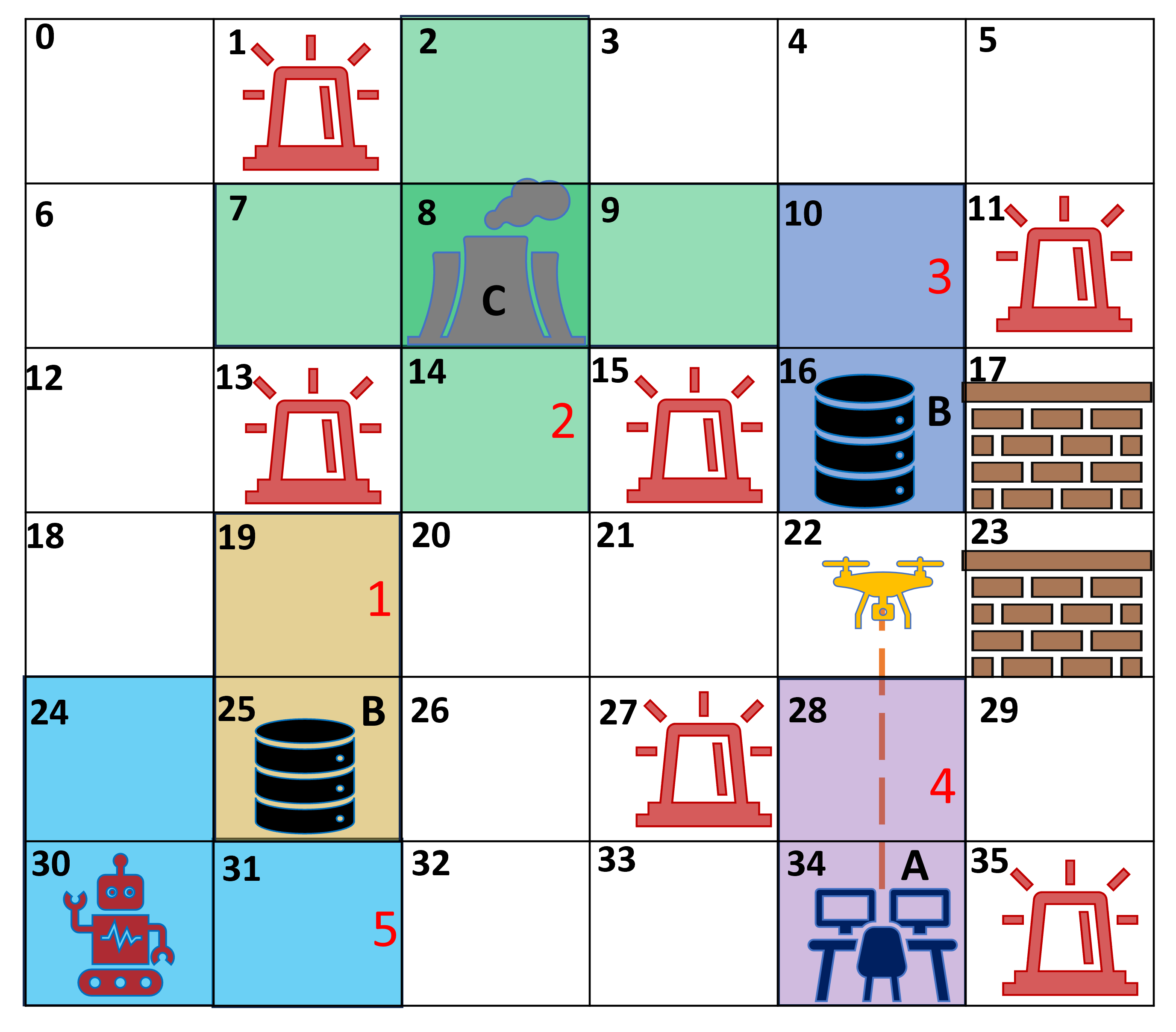
Figure 6: Gridworld depiction of power plant (sensors numbered in red).

Threshold ($\epsilon$)	Prob. Opacity	Exp. Opacity	Exp. Task
0.4	0.6766	0.6678	0.4014
0.6	0.5333	0.5401	0.6021
0.7	0.4611	0.4625	0.7056
0.8	0.3448	0.3359	0.8046
0.95	0.1079	0.1085	0.9504

TABLE IV: Enforced probabilistic opacity and experimental validation.

V-B Transparency enforcement

Consider a case where P1 enforces transparency, in a setup similar to the opacity enforcement case, shown in the Fig. 7. The environment includes one data center ($\mathbf{B}$) in the cell $25$ and a control center ($\mathbf{A}$) in the cell $34$. Three sensors are present: sensor $\mathbf{1}$ a static precision sensor that monitors the cells $30$ and $31$, sensor $\mathbf{2}$ a static binary sensor that monitors the cells $2,8,9,14$, and sensor $\mathbf{3}$ a static binary sensor covering the cells $10$ and $16$. Additionally, the drone, operates between the cells $34$ and $22$ with probabilities of flying to next cell with probability $0.65$ and stay with $0.35$.

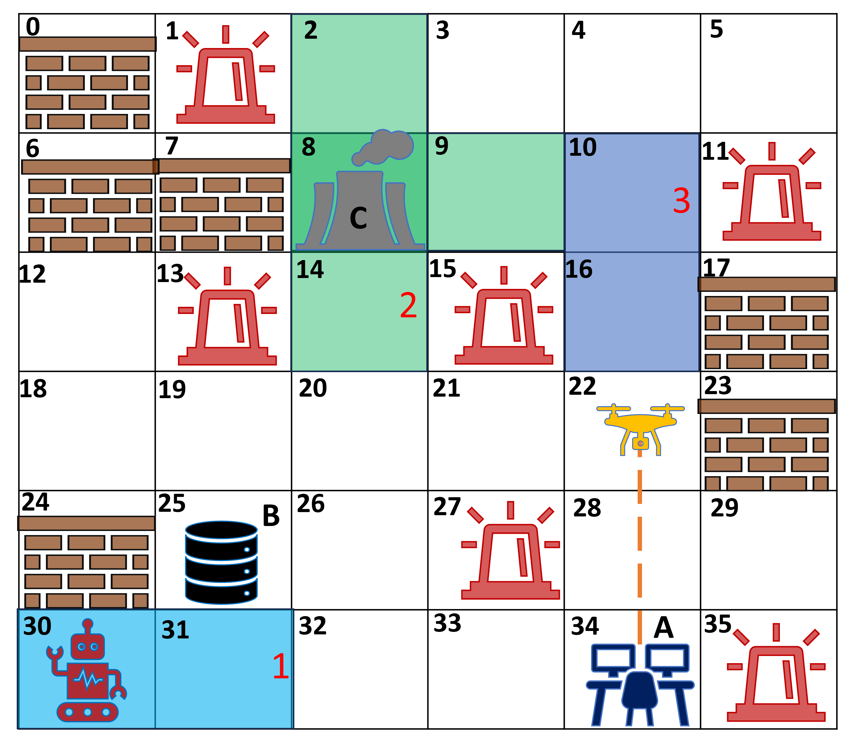
Figure 7: Gridworld depiction for enforcing transparency.

The robot maintains the previous task specification $\psi=\Diamond\,\mathbf{C}$, and P1’s specification for transparency on P2 is $\varphi=\Diamond\,\mathbf{B}\land\Diamond\,\mathbf{A}$.

Table V summarizes transparency enforcement probabilities at various task specification threshold. It also presents the results for P1 following the optimal policy.

Threshold ($\epsilon$)	Prob. Transp.	Exp. Transp.	Exp. Task
0.4	0.8795	0.8784	0.4022
0.6	0.6802	0.6814	0.5999
0.7	0.5581	0.5623	0.7012
0.8	0.4100	0.4105	0.8064
0.95	0.1204	0.1198	0.9503

TABLE V: Enforced probabilistic transparency and validation.

VI Conclusion

We introduced constrained probability planning methods for MDPs to optimize opacity/transparency under task constraints. Our approach starts with building computation models based on FST to capture the observation function of the observer that maps the input languages — state trajectories into the output languages — observed trajectories. Then, by performing the product operations between the FST and the DFA accepting the secret, we can derive another DFA that accepts all possible observations that enforce the opacity of the secret to the observer. Thus, we can formulate the probabilistic planning with opacity as a constrained MDP, augmented with the task state and the state in the DFA of the opaque observations. The dual problem of transparency, can be solved by replacing the maximization with a minimization in the objective function for the constrained MDP. Through experimental analysis, we investigated the impact of sensors and sensor configurations on opacity and transparency enforcement. The construction of opaque/transparent observations can be extended for optimizing opacity in partially observable systems or games with partial observations, involving both collaborative and competitive interactions.

References

- [1] C. Baier and J.-P. Katoen. Principles of model checking. MIT press, 2008.
- [2] B. Bérard, K. Chatterjee, and N. Sznajder. Probabilistic opacity for markov decision processes. Information Processing Letters, 115(1):52–59, 2015.
- [3] B. Bérard, J. Mullins, and M. Sassolas. Quantifying opacity. Mathematical Structures in Computer Science, 25(2):361–403, 2015.
- [4] J. W. Bryans, M. Koutny, L. Mazaré, and P. Y. Ryan. Opacity generalised to transition systems. International Journal of Information Security, 7:421–435, 2008.
- [5] J. W. Bryans, M. Koutny, and P. Y. Ryan. Modelling opacity using petri nets. Electronic Notes in Theoretical Computer Science, 121:101–115, 2005.
- [6] F. Cassez, J. Dubreil, and H. Marchand. Synthesis of opaque systems with static and dynamic masks. Formal Methods in System Design, 40:88–115, 2012.
- [7] G. De Giacomo and M. Y. Vardi. Linear temporal logic and linear dynamic logic on finite traces. In Proceedings of the Twenty-Third international joint conference on Artificial Intelligence, pages 854–860. ACM, 2013.
- [8] C. Keroglou and C. N. Hadjicostis. Probabilistic system opacity in discrete event systems. Discrete Event Dynamic Systems, 28:289–314, 2018.
- [9] F. Lin. Opacity of discrete event systems and its applications. Automatica, 47(3):496–503, 2011.
- [10] S. Liu, X. Yin, D. V. Dimarogonas, and M. Zamani. On approximate opacity of stochastic control systems. arXiv preprint arXiv:2401.01972, 2024.
- [11] B. Maubert, S. Pinchinat, and L. Bozzelli. Opacity issues in games with imperfect information. arXiv preprint arXiv:1106.1233, 2011.
- [12] L. Mazaré. Using unification for opacity properties. Proceedings of the 4th IFIP WG1, 7:165–176, 2004.
- [13] A. Saboori. Verification and enforcement of state-based notions of opacity in discrete event systems. University of Illinois at Urbana-Champaign, 2010.
- [14] A. Saboori and C. N. Hadjicostis. Notions of security and opacity in discrete event systems. In IEEE Conference on Decision and Control, pages 5056–5061, 2007.
- [15] A. Saboori and C. N. Hadjicostis. Verification of initial-state opacity in security applications of des. In 9th International Workshop on Discrete Event Systems, pages 328–333. IEEE, 2008.
- [16] A. Saboori and C. N. Hadjicostis. Opacity-enforcing supervisory strategies via state estimator constructions. IEEE Transactions on Automatic Control, 57(5):1155–1165, 2012.
- [17] A. Saboori and C. N. Hadjicostis. Current-state opacity formulations in probabilistic finite automata. IEEE Transactions on Automatic Control, 59(1):120–133, 2014.
- [18] S. Udupa, H. Rahmani, and J. Fu. Opacity-enforcing active perception and control against eavesdropping attacks. In International Conference on Decision and Game Theory for Security, pages 329–348. Springer, 2023.
- [19] Y.-C. Wu and S. Lafortune. Comparative analysis of related notions of opacity in centralized and coordinated architectures. Discrete Event Dynamic Systems, 23(3):307–339, 2013.
- [20] Y.-C. Wu and S. Lafortune. Synthesis of insertion functions for enforcement of opacity security properties. Automatica, 50(5):1336–1348, 2014.
- [21] Y. Xie, X. Yin, and S. Li. Opacity enforcing supervisory control using nondeterministic supervisors. IEEE Transactions on Automatic Control, 67(12):6567–6582, 2021.
- [22] J. Yao, X. Yin, and S. Li. Sensor deception attacks against initial-state privacy in supervisory control systems. In 2022 IEEE 61st Conference on Decision and Control (CDC), pages 4839–4845. IEEE, 2022.
- [23] X. Yin, Z. Li, W. Wang, and S. Li. Infinite-step opacity and k-step opacity of stochastic discrete-event systems. Automatica, 99:266–274, 2019.
- [24] Y. Zhou, Z. Chen, and Z. Liu. Verification and enforcement of current-state opacity based on a state space approach. European Journal of Control, 71:100795, 2023.