Abstract

Performing inference such a computing confidence intervals is traditionally done, in the parametric case, by first fitting a model and then using the estimates to compute quantities derived at the asymptotic level or by means of simulations such as the ones from the family of bootstrap methods. These methods require the derivation and computation of a consistent estimator that can be very challenging to obtain when the models are complex as is the case for example when the data exhibit some types of features such as censoring, missclassification errors or contain outliers. In this paper, we propose a simulation based inferential method, the implicit bootstrap, that bypasses the need to compute a consistent estimator and can therefore be easily implemented. While being transformation respecting, we show that under similar conditions as for the studentized bootstrap, without the need of a consistent estimator, the implicit bootstrap is first and second order accurate. Using simulation studies, we also show the coverage accuracy of the method with data settings for which traditional methods are computationally very involving and also lead to poor coverage, especially when the sample size is relatively small. Based on these empirical results, we also explore theoretically the case of exact inference.

1 Introduction

1.1 Motivation

In many fields of research ranging from social sciences to life sciences, as well as natural sciences, fitting (parametric) models to data and performing inference such as constructing Confidence Intervals (CIs), is a standard routine. The procedure implies that first a consistent estimator is computed, which is then used to either derive asymptotic distributions or for defining a data generating model used in simulation-based methods, such as the (parametric) bootstrap (Efron and Tibshirani, 1994; DiCiccio and Efron, 1996). This process can become very cumbersome, if not impossible to conduct, when the models are complex, which is the case, for example, when the data have particular features such as measurement disturbances (e.g., outliers, missclassification errors), complex dependence structures, or missing data (e.g., censoring), to name just a few. In these cases the data features have to be taken into account when deriving a consistent estimator, which result in an optimization problem that is numerically challenging to solve. For these complex models, the numerical challenges to obtain consistent estimators result from algorithms with numerical approximations steps, as can be the case, for example, with the Expectation-Maximization (EM) algorithm (Dempster et al., 1977), or involved simulations as is for example the case with indirect inference (Gouriéroux et al., 1993; Smith, 1993). Hence, using a simulation-based method to perform some type of inference, can become impossible in practice, and some simplifications are often needed (see e.g., Honoré and Hu, 2017 and the references therein), with sometimes even inaccurate results (see e.g., Andrews and Buchinsky, 2000). On the other hand, estimating asymptotic covariance matrices is not necessarily easier, and inference based on asymptotic theory is not, in general, second order accurate (see e.g., Hall, 1992). Additionally, consistent estimators can be severely biased in finite samples (see e.g., Kosmidis and Firth, 2009; Kosmidis, 2014; Zhang et al., 2023), and this bias is reported in the estimation of the asymptotic covariance matrix, leading to relatively poor inference.

In this paper, we propose a simulation-based method, the implicit bootstrap, that allows to bypass the need of a consistent point estimator. Namely, we propose to construct a distribution, the implicit bootstrap distribution, from which we derive CIs using the percentile method. We show that, under some regularity conditions, the one-sided percentile intervals are valid and can even be second-order accurate in the sense that the coverage of the interval has the correct nominal coverage level up to an error of order $o(n^{-\nicefrac{{1}}{{2}}})$. This results shows that no additional adjustment is needed, as it would be the case for a parametric bootstrap (Efron, 1987). Moreover, the percentile method has the notable advantage to be transformation respecting (Efron and Tibshirani, 1994). Although the implicit bootstrap is a computer intensive procedure, it is particularly fast when considering continuous parametric models and initial estimators that can be written as the solution of an estimating equation ($Z$-estimator).

1.2 Results and contributions

Assuming that observed data are generated from $F_{{\bm{\theta}}_{0}}$, where ${\bm{\theta}}_{0}\in{\bm{\Theta}}\subset{}^{p}$, our goal is to construct valid CIs for the individual components of ${\bm{\theta}}_{0}$ or, in most case, for suitable functions of ${\bm{\theta}}_{0}$.

The implicit bootstrap relies on an initial readily available estimator $\widehat{{\bm{\pi}}}_{n}({\bm{\theta}}_{0})$ typically chosen for its numerical simplicity. This estimator is computed on a random sample denoted by ${\bf Y}({\bm{\theta}}_{0})\in{}^{n}$. We assume that data can be simulated or synthetically generated from $F_{{\bm{\theta}}}$ for any ${\bm{\theta}}\in{\bm{\Theta}}$. More specifically, we express the parametric data generating mechanism as ${\bf Y}({\bm{\theta}})\vcentcolon=\mathbf{F}({\bm{\theta}},\!{\bf W})$ where ${\bf W}=[\text{W}_{i}]_{i=1,\ldots,n}$, $\text{W}_{i}$ is a random variable whose distribution does not depend on ${\bm{\theta}}$, i.e., for all ${\bm{\theta}}\in{\bm{\Theta}}$, and all $x\in\real$, $\Pr(\text{W}_{i}\leq x\mid{\bm{\theta}})=\Pr(\text{W}_{i}\leq~{}x)$. As a simple example, if ${\bf Y}({\bm{\theta}})=\{Y_{1}({\bm{\theta}}),\dots,Y_{n}({\bm{\theta}})\}^{\top}$ and $Y_{i}({\bm{\theta}})$ are continuous i.i.d. random variables, then one can think of $\mathbf{F}({\bm{\theta}},\!{\bf W})$ as $(\text{F}_{\bm{\theta}}^{-1}(\text{W}_{1}),\dots,\text{F}_{\bm{\theta}}^{-1}(\text{W}_{n}))^{\top}$ where $\text{F}_{\bm{\theta}}^{-1}$ is the quantile function and $W_{i}$ are independent $U(0,1)$. In order to construct CIs for the components of ${\bm{\theta}}_{0}$, or suitable functions of ${\bm{\theta}}_{0}$, we propose to use the distribution of $\widecheck{\bm{\theta}}_{n}^{\ast}$, with

$$\widecheck{\bm{\theta}}_{n}^{\ast}\in\operatorname*{argmin}_{{\bm{\theta}}\in{\bm{\Theta}}_{1}}\;\|\widehat{{\bm{\pi}}}_{n}-\widehat{{\bm{\pi}}}_{n}^{*}({\bm{\theta}})\|,$$ (1)

where $\widehat{{\bm{\pi}}}_{n}\vcentcolon=\widehat{{\bm{\pi}}}_{n}({\bm{\theta}}_{0})$ and $\widehat{{\bm{\pi}}}_{n}^{*}({\bm{\theta}})$ is computed on the simulated sample ${\bf Y}^{*}({\bm{\theta}})=\mathbf{F}({\bm{\theta}},{\bf W}^{*})$ with ${\bf W}^{\ast}$ being an independent copy of ${\bf W}$, and ${\bm{\Theta}}_{1}\subset{\bm{\Theta}}$ is a suitable subspace that contains ${\bm{\theta}}_{0}$ in its interior. Specific requirements on ${\bm{\Theta}}_{1}$ are discussed in Section 2.2.

Eq. 1 can be expressed more formally considering that ${\bf W}$ is a random variable/vector and the estimators $\widehat{{\bm{\pi}}}_{n}({\bm{\theta}})$ and $\widehat{{\bm{\pi}}}_{n}^{\ast}({\bm{\theta}})$, with ${\bm{\theta}}\in{\bm{\Theta}}$, correspond to a map $\widehat{{\bm{\pi}}}_{n}({\bm{\theta}},\cdot)$ such that $\widehat{{\bm{\pi}}}_{n}({\bm{\theta}})\vcentcolon=\widehat{{\bm{\pi}}}_{n}({\bm{\theta}},{\bf W})$ and $\widehat{{\bm{\pi}}}_{n}^{\ast}({\bm{\theta}})\vcentcolon=\widehat{{\bm{\pi}}}_{n}({\bm{\theta}},{\bf W}^{\ast})$. Hence, $\widecheck{\bm{\theta}}_{n}^{\ast}$ correspond to a map $\widecheck{\bm{\theta}}_{n}(\cdot,\cdot)$ that is such that, for (almost) all realisations w and $\textbf{w}^{\ast}$ of ${\bf W}$ and ${\bf W}^{\ast}$ respectively,

$$\widecheck{\bm{\theta}}_{n}(\textbf{w},\textbf{w}^{\ast})\in\operatorname*{argmin}_{{\bm{\theta}}\in{\bm{\Theta}}_{1}}\;\|\widehat{{\bm{\pi}}}_{n}({\bm{\theta}}_{0},\textbf{w})-\widehat{{\bm{\pi}}}_{n}({\bm{\theta}},\textbf{w}^{\ast})\|.$$ (2)

Formal justifications to ensure that Eq. 2 is well-defined will be provided in Section 2.2.

In this paper, we show that the implicit bootstrap, under mild and standard regularity conditions, provides valid CIs for suitable real-valued functions of ${\bm{\theta}}_{0}$. More precisely, throughout this paper we will consider $\vartheta\vcentcolon=\psi({\bm{\theta}})$ with $\psi:{\bm{\Theta}}\to\real$ being a differentiable function, e.g., $\psi({\bm{\theta}})={\bf s}^{\top}{\bm{\theta}}$ where ${\bf s}$ is a canonical basis vector of ^p. Let $\vartheta_{0}\vcentcolon=\psi({\bm{\theta}}_{0})$ and $\check{\vartheta}^{\ast}_{n}(\alpha)$ correspond to the $\alpha$-level quantile, with $\alpha\in(0,1)$, of the distribution of $\check{\vartheta}_{n}^{\ast}\vcentcolon=\psi(\widecheck{\bm{\theta}}_{n}^{\ast})$, i.e, $\check{\vartheta}^{\ast}_{n}(\alpha)\vcentcolon=\inf\left\{x\in\real\mid\Pr\left(\check{\vartheta}_{n}^{\ast}\leq x\mid\widehat{{\bm{\pi}}}_{n}\right)\geq\alpha\right\}$. Then, under appropriate assumptions,

1. the implicit bootstrap provides first-order accurate CIs, i.e.,

   $$\Pr\{\vartheta_{0}\leq\check{\vartheta}^{\ast}_{n}(\alpha)\}=\alpha+o(1),$$

2. the implicit bootstrap provides second-order accurate CIs, i.e.,

   $$\Pr\{\vartheta_{0}\leq\check{\vartheta}^{\ast}_{n}(\alpha)\}=\alpha+o(n^{-\nicefrac{{1}}{{2}}}),$$

3. finally, under more stringent conditions, the implicit bootstrap provides exact coverage in finite sample, i.e.,

   $$\Pr\{\vartheta_{0}\leq\check{\vartheta}^{\ast}_{n}(\alpha)\}=\alpha.$$

In order to solve Eq. 1, thereby determining the implicit bootstrap estimator $\widecheck{\bm{\theta}}_{n}^{\ast}$, one can use two efficient and easy to implement methods. The iterative bootstrap introduced by Kuk (1995) and discussed in Guerrier et al. (2019) can be used in a large number of situations. Alternatively, if the initial estimator $\widehat{{\bm{\pi}}}_{n}({\bm{\theta}})$ can be expressed as a $Z$-estimator, i.e., the root of a system of nonlinear equations (see Van Der Vaart and Wellner, 1996), we introduce the Switched $Z$-estimator (SwiZ) in Section 3. In particular, we demonstrate under mild conditions that the SwiZ is equivalent to the implicit bootstrap defined in Eq. 1, whereas it has the advantage to be computationally as efficient as solving the implicit bootstrap when $\widehat{{\bm{\pi}}}_{n}({\bm{\theta}})$ has a closed form expression.

1.3 Illustrative example

Queuing models are commonly used in management science and engineering. Depending on what can be observed, the likelihood functions may be difficult to evaluate. In cases where only departure times $y_{1},y_{2},\dots,y_{n}$ are observed, the challenge arises from the fact that the likelihood function is evaluated by integrating over a number of terms that increases exponentially with the sample size. The M/G/1 queue model, where M stands for an exponential distribution and G for another general one, is a popular model that has been examined in previous research by Heggland and Frigessi (2004); Blum and François (2010); Fearnhead and Prangle (2012). In their study, the service times are uniformly distributed (i.e. the G distribution) in the interval $[\theta_{1},\theta_{2}]=[0.3,0.9]$ and the inter-departure times are exponentially distributed with rate $\theta_{3}=1$. For point estimation, Heggland and Frigessi (2004) use two sample statistics as well as the MLE of an auxiliary model (with a closed-form likelihood function) as an auxiliary estimator in the framework of indirect inference. Blum and François (2010) use 20 evenly spaced quantiles of inter-departure times as auxiliary statistics for the Approximate Bayesian Computation (ABC) method, and Fearnhead and Prangle (2012) use the same auxiliary statistics but with a semi-automatic ABC approach.

Obviously, these estimators being quite numerically involved, constructing CIs using simulation based methods is quite prohibitive. Moreover, asymptotic covariance matrices are not necessary known or easy to estimate for all parameters. For this setting, we propose, as initial estimator, the MLE of a location-scale Fréchet distribution for independent observations (Smith, 1985). Arguably, supposing independence of the observations, their marginal distribution can be reasonably fitted using such a probability distribution function, which is characterized by three parameters. The resulting estimator is not a consistent estimator of the M/G/1 queue model’s parameters, but as explained above (see also Section 1.2), the implicit bootstrap is a suitable method for providing accurate CIs in such settings. We consider here a population M/G/1 queue model with $[\theta_{1},\theta_{2}]=[0.3,0.9]$ and rate $\theta_{3}=1$ for the inter-departure times. These selected values correspond to realistic scenarios where the expected service time is moderately shorter than the expected inter-departure time, making a balance to prevent less interesting situations where queues are persistently empty or the system is always busy. We compute CIs for all parameters, using the implicit bootstrap, and as a comparison, we also compute the CIs for the two steps approach which consists in first obtaining a consistent point estimator using an indirect inference inference estimator with the MLE of the Fréchet model as the auxiliary estimator, and then applying the parametric percentile bootstrap. While the later is a valid method, since it is based on a consistent estimator, the numerical procedure is considerably more expensive as each bootstrap estimator is an indirect inference estimator which needs to be computed for each simulated (bootstrapped) sample.

The CIs’ coverage probability and median length for the two methods are presented in LABEL:table:mg1, and are the results of a Monte Carlo simulation with two sample sizes, $n=250,500$, generated from the M/G/1 queue model with ${\bm{\theta}}=(0.3,0.9,1.0)^{\top}$, using $M=10,000$ simulated samples. The table also contains the median computational times for the two methods. Although the statistical performance of the two (valid) methods, in terms of coverage and CIs lengths are comparable, and also quite accurate regarding the coverage, the striking difference lies in the computational time. Indeed, the two-steps approach is about $5000$ times slower than the implicit bootstrap, or, equivalently, the implicit bootstrap is the only computationally viable method for this setting. For larger models, in terms of the number of parameters to estimate, this is even more evidently the case.

Table 1: Empirical coverages in %, median lengths and median computational times (Time) in seconds (s) or hours (h), for two-sided 95% CIs calculated from $10,000$ independent samples from a M/G/1 queue model with ${\bm{\theta}}=(0.3,0.9,1.0)^{\top}$, for varying sizes $n$. The methods are the Implicit Bootstrap (IB) and the two steps method (2-steps) with the indirect inference estimator followed by a parametric percentile bootstrap.

	Coverage (Median Length)			Time
Method	$\theta_{1}$	$\theta_{2}$	$\theta_{3}$
	$n=250$
IB	95.05 (0.041)	97.12 (0.225)	96.47 (0.251)	2.56 s
2-steps	93.13 (0.040)	93.82 (0.240)	94.73 (0.247)	3.68 h
	$n=500$
IB	94.95 (0.028)	95.69 (0.164)	95.66 (0.178)	4.50 s
2-steps	93.90 (0.028)	94.15 (0.172)	94.81 (0.176)	6.74 h

1.4 Organization and notation

The rest of the article is organized as follows. In Section 2, we formally present our method and discuss its first and second order accuracy as well as the exact inference property. In Section 3, we present a particular implementation of our method and show its computational efficiency. In Section 4, we conduct simulation studies and illustrate that our method benefits from advantageous coverage accuracy while being computationally efficient. All the proofs are in the Appendix.

We finish this section with notations that will be used throughout this work.

• We will write $x\vcentcolon=y$ to denote that $x$ is defined as being equal to $y$.

• We will denote $X_{n}\buildrel d\over{\longrightarrow}X$ if $X_{n}$ converge in distribution to $X$. The symbol $\buildrel d\over{\longrightarrow}$ will be replaced by $\buildrel p\over{\longrightarrow}$ or $\buildrel a.s.\over{\longrightarrow}$, to denote the convergence in probability or the almost sure convergence, respectively.

• We will denote $X\overset{d}{=}Y$ if $X$ has the same distribution as $Y$.

• For $x\in{}^{p}$, we will denote by $\|x\|$ its Euclidean norm.

2 The implicit bootstrap

In this section, we first present the intuitive idea behind the implicit bootstrap and then develop, successively, the conditions for first and second order properties to hold, as well as those for exact inference. The proofs are provided in the Appendix.

2.1 Intuitive Idea of the Implicit Bootstrap

Recall that the implicit bootstrap relies on an initial readily available estimator $\widehat{{\bm{\pi}}}_{n}({\bm{\theta}}_{0})$, typically chosen for its numerical simplicity. While the initial estimator is not required to be consistent for ${\bm{\theta}}_{0}$ we assume that it converges to a non-stochastic limit ${\bm{\pi}}({\bm{\theta}}_{0})$ and that the function ${\bm{\pi}}({\bm{\theta}})$ is one-to-one in ${\bm{\Theta}}_{1}$. Under standard technical requirements which for simplicity are assumed throughout the rest of this section, we can define the idealized estimator $\widehat{{\bm{\theta}}}_{n}\vcentcolon=~{}\bm{\pi}^{-1}\left\{\widehat{{\bm{\pi}}}_{n}({\bm{\theta}}_{0})\right\}$. This estimator is related to indirect inference estimators (Gouriéroux et al., 1993, 2000) in the sense that the latter are defined as an approximate solution of the equation ${\bm{\pi}}({\bm{\theta}})=\widehat{{\bm{\pi}}}_{n}({\bm{\theta}}_{0})$. We have that $\widehat{{\bm{\theta}}}_{n}$ is consistent for ${\bm{\theta}}_{0}$ by the continuous mapping theorem and is asymptotically normal when the initial estimator is so, by the delta method. Namely, we have that

$$~{}n^{\nicefrac{{1}}{{2}}}{\bf\Sigma}({\bm{\theta}}_{0})^{-\nicefrac{{1}}{{2}}}\left(\widehat{{\bm{\theta}}}_{n}-{\bm{\theta}}_{0}\right)\overset{d}{\to}\mathcal{N}(\bm{0},{\bf I}_{p}),$$ (3)

where $\bm{0}$ is the zero vector in ^p and ${\bf I}_{p}$ is the $p\times p$ identity matrix and ${\bf\Sigma}({\bm{\theta}}_{0})$ is the covariance matrix of $\widehat{{\bm{\theta}}}_{n}$. To construct CIs for components of ${\bm{\theta}}_{0}$, one could consider the distribution of $\widecheck{\bm{\theta}}_{n}^{\ast}$, with

$$~{}\widecheck{\bm{\theta}}_{n}^{\ast}=\operatorname*{argzero}_{{\bm{\theta}}\in{\bm{\Theta}}_{1}}\;\widehat{{\bm{\theta}}}_{n}-\widehat{{\bm{\theta}}}_{n}^{*}({\bm{\theta}}),$$ (4)

where $\widehat{{\bm{\theta}}}_{n}^{*}({\bm{\theta}})\vcentcolon={\bm{\pi}}^{-1}\{\widehat{{\bm{\pi}}}_{n}^{\ast}({\bm{\theta}})\}$. Considering the distribution of $\widecheck{\bm{\theta}}_{n}^{\ast}$, conditional on $\widehat{{\bm{\theta}}}_{n}$, and the bootstrap distribution $\widehat{{\bm{\theta}}}_{n}^{\ast}\vcentcolon=\widehat{{\bm{\theta}}}_{n}^{\ast}(\widehat{{\bm{\theta}}}_{n})$, also conditional on $\widehat{{\bm{\theta}}}_{n}$, we can show under regularity conditions that

$$~{}n^{\nicefrac{{1}}{{2}}}{\bf\Sigma}(\widehat{{\bm{\theta}}}_{n})^{-\nicefrac{{1}}{{2}}}\left(\widecheck{\bm{\theta}}_{n}^{\ast}-\widehat{\bm{\theta}}_{n}\right)\overset{d}{\to}\mathcal{N}(\bm{0},{\bf I}_{p})\quad\text{and}\quad n^{\nicefrac{{1}}{{2}}}{\bf\Sigma}(\widehat{{\bm{\theta}}}_{n})^{-\nicefrac{{1}}{{2}}}\left(\widehat{{\bm{\theta}}}_{n}^{*}-\widehat{{\bm{\theta}}}_{n}\right)\overset{d}{\to}\mathcal{N}(\bm{0},{\bf I}_{p}),$$ (5)

in probability. Hence, the distribution of $\widecheck{\bm{\theta}}_{n}^{\ast}$ acts like the bootstrap distribution $\widehat{{\bm{\theta}}}_{n}^{*}$ of the implicit estimator $\widehat{{\bm{\theta}}}_{n}$. For this reason, we call $\widecheck{\bm{\theta}}_{n}^{\ast}$ the implicit bootstrap estimator. Given Eq. 5, the validity of our approach, as well as the validity of Efron’s percentile bootstrap, is justified by Lemma 23.3 in Van der Vaart, 1998.

However, in practice, the function ${\bm{\pi}}({\bm{\theta}})$ is unknown, but by construction, a solution of (4) can equivalently be obtained by solving in ${\bm{\theta}}$, $\widehat{{\bm{\pi}}}_{n}({\bm{\theta}}_{0})=\widehat{{\bm{\pi}}}_{n}^{*}({\bm{\theta}})$, i.e.

$$\widecheck{\bm{\theta}}_{n}^{\ast}=\operatorname*{argzero}_{{\bm{\theta}}\in{\bm{\Theta}}_{1}}\;\widehat{{\bm{\theta}}}_{n}({\bm{\theta}}_{0})-\widehat{{\bm{\theta}}}_{n}^{*}({\bm{\theta}})=\operatorname*{argzero}_{{\bm{\theta}}\in{\bm{\Theta}}_{1}}\;\widehat{{\bm{\pi}}}_{n}({\bm{\theta}}_{0})-\widehat{{\bm{\pi}}}_{n}^{\ast}({\bm{\theta}}).$$ (6)

In Appendix A, we provide comparisons with alternative related methods, i.e. indirect inference and generalized fiducial inference.

2.2 1st order Validity

The first assumption imposes requirements on the subspace ${\bm{\Theta}}_{1}$ of the parameter space ${\bm{\Theta}}$.

Assumption 1:

The space ${\bm{\Theta}}_{1}$ is compact, convex and such that ${\bm{\theta}}_{0}\in\operatorname*{Int}({\bm{\Theta}}_{1})$.

1 is a common regularity condition typically when $\widehat{{\bm{\pi}}}_{n}({\bm{\theta}})$ is not known in closed form (see e.g., Newey and McFadden, 1994). This condition is rather mild since it is not made on the whole parameter space ${\bm{\Theta}}$ but on a subspace that can be chosen. The substantial part of this assumption is that ${\bm{\theta}}_{0}$ is not on the boundary of the parameter space. The next assumption, imposes requirements on the asymptotic bias function ${\bm{\pi}}({\bm{\theta}})$.

Assumption 2:

The function ${\bm{\pi}}({\bm{\theta}})$, restricted to ${\bm{\Theta}}_{1}$, is a homeomorphism, continuously differentiable and the Jacobian matrix $\bm{A}({\bm{\theta}})\vcentcolon=\partial{\bm{\pi}}({\bm{\theta}})/\partial{\bm{\theta}}$ has full rank for any ${\bm{\theta}}\in{\bm{\Theta}}_{1}$.

A map is a homeomorphism if it is continuous with a continuous inverse. In particular, such map is injective. The injectivity requirement on ${\bm{\pi}}({\bm{\theta}})$ is a common regularity condition for identifiability (see e.g., Gouriéroux et al., 2000 and references therein). Primitive conditions that ensure such property can be found for example in Gale and Nikaido (1965) or Komunjer (2012). The smoothness and full rank requirements are rather mild and are commonly considered for indirect inference estimators, where ${\bm{\pi}}$ is called the binding function (see e.g., Gouriéroux et al., 1993), and can be satisfied for example when the data exhibit features such as censoring with the initial estimator being the ordinary least square estimator (see e.g., Greene, 1981).

The third assumption describes the asymptotic behavior of the initial estimator.

Assumption 3:

There exist a diverging sequence of positive numbers $\{a_{n}\}_{n\geqslant 1}$ and a random vector $\mathbf{Z}$ whose distribution is continuous and does not depend on ${\bm{\theta}}\in{\bm{\Theta}}$, such that we have, uniformly in ${\bm{\theta}}\in{\bm{\Theta}}_{1}$,

$$a_{n}\bm{\Sigma}_{n}({\bm{\theta}})^{-\nicefrac{{1}}{{2}}}\{\widehat{{\bm{\pi}}}_{n}({\bm{\theta}})-{\bm{\pi}}({\bm{\theta}})\}\buildrel d\over{\longrightarrow}\mathbf{Z},$$

where $\bm{\Sigma}_{n}({\bm{\theta}})\vcentcolon=\hbox{cov}\{a_{n}\widehat{{\bm{\pi}}}_{n}({\bm{\theta}})\}$ is the covariance. Moreover, the sequence $\{\bm{\Sigma}_{n}({\bm{\theta}})\}_{n\geq 1}$ converges uniformly in ${\bm{\theta}}\in{\bm{\Theta}}_{1}$ to a positive definite matrix $\bm{\Sigma}({\bm{\theta}})$ which is continuous in ${\bm{\theta}}\in{\bm{\Theta}}_{1}$.

In most cases, $\mathbf{Z}$ follows a standard normal distribution and $a_{n}=n^{\nicefrac{{1}}{{2}}}$. In this particular case and when $\widehat{\bm{\theta}}_{n}({\bm{\theta}})=\widehat{{\bm{\pi}}}_{n}({\bm{\theta}})$, i.e., the initial estimator is consistent, sufficient conditions guaranteeing that 3 holds are given in Sweeting (1980). Moreover, the uniformity requirement is equivalent to the following: for any sequence $\{{\bf x}_{n}\}\subset{\bm{\Theta}}_{1}$

$$~{}a_{n}\bm{\Sigma}_{n}({\bm{\theta}})^{-\nicefrac{{1}}{{2}}}\{\widehat{{\bm{\pi}}}_{n}({\bf x}_{n})-{\bm{\pi}}({\bf x}_{n})\}\buildrel d\over{\longrightarrow}\mathbf{Z}.$$ (7)

When ${\bm{\pi}}({\bm{\theta}})$ is the identity, i.e., $\widehat{\bm{\theta}}_{n}({\bm{\theta}})=\widehat{{\bm{\pi}}}_{n}({\bm{\theta}})$, Eq. 7 immediately implies that

$$a_{n}\bm{\Sigma}_{n}({\bm{\theta}}_{0})^{-\nicefrac{{1}}{{2}}}\left(\widehat{\bm{\theta}}_{n}-{\bm{\theta}}_{0}\right)\buildrel d\over{\longrightarrow}\mathbf{Z},\quad\text{and}\quad a_{n}\bm{\Sigma}_{n}(\widehat{\bm{\theta}}_{n})^{-\nicefrac{{1}}{{2}}}\left(\widehat{\bm{\theta}}_{n}^{\ast}-\widehat{\bm{\theta}}_{n}\right)\buildrel d\over{\longrightarrow}\mathbf{Z},\,\text{in probability,}$$

which is an essential requirement of Lemma 23.3 in Van der Vaart, 1998. As previously said, the latter result ensures the validity of Efron’s percentile bootstrap. More generally, uniform convergence requirements are regularity conditions that are often imposed to show consistency or asymptotic normality in parametric statistical procedures, such as in indirect inference (see e.g., Newey, 1991; Phillips, 2012; Arvanitis and Demos, 2018; Kasy, 2019).

Theorem 1 below states the 1st order property of our approach and is proved in Section B.1.

Theorem 1:

Let $\alpha\in(0,1)$. Then, under Assumptions 1 to 3, we have,

$$\Pr\{\vartheta_{0}\leq\check{\vartheta}^{\ast}_{n}(\alpha)\}=\alpha+o(1).$$

Remark A:

Contrary to the percentile bootstrap, the implicit bootstrap method does not require the asymptotic distribution of $\check{\vartheta}_{n}^{\ast}$, nor the one of $\widecheck{\bm{\theta}}_{n}^{\ast}$, to be symmetric (see e.g., Van der Vaart, 1998, Lemma 23.3). This is mainly due to the fact that, using Assumptions 1 to 3, we can show that

$$a_{n}\bm{\Sigma}_{n}(\widehat{\bm{\theta}}_{n})^{-\nicefrac{{1}}{{2}}}\bm{A}(\widehat{\bm{\theta}}_{n})\left(\widecheck{\bm{\theta}}^{\ast}_{n}-\widehat{\bm{\theta}}_{n}\right)\overset{d}{\longrightarrow}-\mathbf{Z},$$

conditionally on $\widehat{\bm{\theta}}_{n}$ in probability; see 4 in Section B.1.

Remark B:

A result interesting in of itself, that we derive to prove 1, is a uniform extension of Skorokhod’s representation theorem. More precisely, under 3, let ${\bf X}_{n}({\bm{\theta}})\vcentcolon=a_{n}{\bf\Sigma}_{n}({\bm{\theta}})^{-\nicefrac{{1}}{{2}}}\{\widehat{{\bm{\pi}}}_{n}({\bm{\theta}})-{\bm{\pi}}({\bm{\theta}})\}$, for each ${\bm{\theta}}\in{\bm{\Theta}}_{1}$. Then, there exists, for each ${\bm{\theta}}\in{\bm{\Theta}}_{1}$, a random sequence $\widetilde{{\bf X}}_{n}({\bm{\theta}})$ such that

1. $\widetilde{{\bf X}}_{n}({\bm{\theta}})\overset{\text{a.s.}}{\longrightarrow}{\bf Z}$ uniformly in ${\bm{\theta}}\in{\bm{\Theta}}_{1}$,

2. $\widetilde{{\bf X}}_{n}({\bm{\theta}})\overset{d}{=}{\bf X}_{n}({\bm{\theta}})$, for each $n\in\mathbb{N}$ and each ${\bm{\theta}}\in{\bm{\Theta}}_{1}$.

The almost sure convergence implies that, without loss of generality, a common sample space ${\bm{\Omega}}$ can be considered for the entire family of random vectors $\{\widehat{{\bm{\pi}}}_{n}({\bm{\theta}})\}_{n\in\mathbb{N},{\bm{\theta}}\in{\bm{\Theta}}_{1}}$, thereby justifying the definition of $\widecheck{\bm{\theta}}_{n}^{\ast}$ put forward in Eq. 2. This result and its proof are provided in Section B.1. Other uniform extension of classical results, such as the continuous mapping theorem, the delta method or central limit theorem, can be found in Kasy, 2019.

2.3 2nd order Validity

In order to demonstrate that $\alpha$-level quantiles of the implicit bootstrap distribution $\check{\vartheta}^{\ast}_{n}$ are second order accurate, we rely on the theory developed in Hall, 1992. The latter, through the theory of Edgeworth expansion, provides the justification of the 2nd order property of the studentized bootstrap method, while also showing why the percentile bootstrap method and the classic asymptotic theory are only 1st order. We will show that, when the magnitude of the error in Eq. 1 is small enough, similar assumptions lead to the 2nd order property of the implicit bootstrap method.

We start with two assumptions that are stronger versions of Assumptions 2 and 3 and ensure that $\operatorname*{argmin}_{{\bm{\theta}}\in{\bm{\Theta}}_{1}}\|\widehat{{\bm{\pi}}}_{n}-\widehat{{\bm{\pi}}}_{n}^{\ast}({\bm{\theta}})\|$ is “small enough”. We should highlight that if a perfect matching is always possible, i.e., there always exists a $\widecheck{\bm{\theta}}_{n}^{\ast}$ such that $\|\widehat{{\bm{\pi}}}_{n}-\widehat{{\bm{\pi}}}_{n}^{\ast}(\widecheck{\bm{\theta}}_{n}^{\ast})\|=0$, then  4 and 5 below are unnecessary.

Assumption 4:

The function ${\bm{\pi}}({\bm{\theta}})$, restricted to ${\bm{\Theta}}_{1}$, is a diffeomorphism and the Jacobian matrix $\bm{A}({\bm{\theta}})\vcentcolon=\partial{\bm{\pi}}({\bm{\theta}})/\partial{\bm{\theta}}$ has full rank for any ${\bm{\theta}}\in{\bm{\Theta}}_{1}$.

A map is a diffeomorphism if it is continuously differentiable with a continuously differentiable inverse. We immediately see that 4 implies 2. The essential distinction between these two assumptions is that the former allows us to make use of the mean value theorem with the map ${\bm{\pi}}^{-1}$.

For the next assumption, we require first that 3 holds true. As explained in B, we can without loss of generality assume that a common sample space ${\bm{\Omega}}$ can be considered for the random vectors ${\bf X}_{n}({\bm{\theta}})=a_{n}{\bf\Sigma}_{n}({\bm{\theta}})^{-\nicefrac{{1}}{{2}}}\{\widehat{{\bm{\pi}}}_{n}({\bm{\theta}})-{\bm{\pi}}({\bm{\theta}})\}$ as well as ${\bf Z}$. As a consequence, the following map can be considered for any $n\in\mathbb{N}$ and ${\bm{\theta}}\in{\bm{\Theta}}_{1}$,

$$~{}\begin{array}[]{rcl}\mathcal{R}_{n}({\bm{\theta}}):{\bm{\Omega}}&\to&{}^{p}\\ \bm{\omega}&\mapsto&\widetilde{\bf X}_{n}({\bm{\theta}},\bm{\omega})-{\bf Z}(\bm{\omega}),\end{array}$$ (8)

where $\widetilde{\bf X}_{n}({\bm{\theta}})\buildrel a.s.\over{\longrightarrow}{\bf Z}$ uniformly in ${\bm{\theta}}\in{\bm{\Theta}}_{1}$. As a consequence, we have $\mathcal{R}_{n}({\bm{\theta}})=o(1)$ almost surely, uniformly in ${\bm{\theta}}\in{\bm{\Theta}}_{1}$. In the following assumption, we require a specific order for this map as well as a continuity property.

Assumption 5:

3 holds and the components of the matrix ${\bf\Sigma}({\bm{\theta}})$ are continuously differentiable in ${\bm{\theta}}\in{\bm{\Theta}}_{1}$. Moreover, the family $\{\mathcal{R}_{n}({\bm{\theta}})\}_{n\in\mathbb{N}}$ given in Eq. 8 is equicontinuous in ${\bm{\theta}}\in{\bm{\Theta}}_{1}$ for almost all $\bm{\omega}\in{\bm{\Omega}}$ and, the map $\mathcal{R}_{n}({\bm{\theta}})$ is such that $\mathcal{R}_{n}({\bm{\theta}},\bm{\omega})=\mathcal{O}(n^{-\nicefrac{{1}}{{2}}})$ for almost all $\bm{\omega}\in{\bm{\Omega}}$.

Since ${\bm{\Theta}}_{1}$ is compact by 1, the equicontinuity requirement on $\{\mathcal{R}_{n}({\bm{\theta}})\}_{n\in\mathbb{N}}$ implies that this family is uniformly equicontinuous on ${\bm{\Theta}}_{1}$, for almost all $\bm{\omega}\in{\bm{\Omega}}$. Therefore, for any sequences $\{{\bf x}_{n}\},\{{\bf y}_{n}\}\subset{\bm{\Theta}}_{1}$ such that $\|{\bf x}_{n}-{\bf y}_{n}\|=o(1)$, we have $\|\mathcal{R}_{n}({\bf x}_{n},\bm{\omega})-\mathcal{R}_{n}({\bf y}_{n},\bm{\omega})\|=o(n^{-\nicefrac{{1}}{{2}}})$, for almost all $\bm{\omega}\in{\bm{\Omega}}$. Similarly to uniformity, (stochastic) equicontinuity requirements are common regularity conditions used in parametric statistical procedures (see e.g., Newey, 1991; Andrews, 1992).

Using the previous two assumptions with 1, we have the following result.

Lemma 1:

Under Assumptions 1, 4 and 5 we have $\operatorname*{argmin}_{{\bm{\theta}}\in{\bm{\Theta}}_{1}}\|\widehat{{\bm{\pi}}}_{n}({\bm{\theta}}_{0})-\widehat{{\bm{\pi}}}_{n}^{\ast}({\bm{\theta}})\|=~{}o_{p}(n^{-1}).$

The proof of 1 is provided in Section B.2.

Before stating the next assumption, we introduce some notations that we will use throughout this section. We write $\widehat{\bm{\theta}}_{n}^{\ast\ast}\vcentcolon={\bm{\pi}}^{-1}\{\widehat{{\bm{\pi}}}_{n}^{\ast\ast}(\widecheck{\bm{\theta}}_{n}^{\ast})\}$ where $\widehat{{\bm{\pi}}}_{n}^{\ast\ast}(\widecheck{\bm{\theta}}_{n}^{\ast})$ is computed on the simulated sample ${\bf Y}^{\ast\ast}(\widecheck{\bm{\theta}}_{n}^{\ast})=\mathbf{F}(\widecheck{\bm{\theta}}_{n}^{\ast},{\bf W}^{\ast\ast})$, where ${\bf W}^{\ast\ast}$ is an independent copy of ${\bf W}$. We denote $\hat{\vartheta}_{n}\vcentcolon=\psi(\widehat{\bm{\theta}}_{n})$ and $\hat{\vartheta}_{n}^{\ast\ast}\vcentcolon=\psi(\widehat{\bm{\theta}}_{n}^{\ast\ast})$. From the assumptions and the results of the previous section, we can deduce that for any ${\bm{\theta}}\in\operatorname*{Int}({\bm{\Theta}}_{1})$, the asymptotic variance of $\psi\{\widehat{\bm{\theta}}_{n}({\bm{\theta}})\}$ is given by

$$\varsigma({\bm{\theta}})^{2}\vcentcolon=\frac{\partial\psi}{\partial{\bm{\theta}}}({\bm{\theta}})^{\top}\{\bm{A}({\bm{\theta}})^{-1}\}^{\top}{\bf\Sigma}({\bm{\theta}})\bm{A}({\bm{\theta}})^{-1}\frac{\partial\psi}{\partial{\bm{\theta}}}({\bm{\theta}}),$$

and $\varsigma(\widehat{\bm{\theta}}_{n})^{2}$ is a consistent estimator of $\varsigma({\bm{\theta}}_{0})^{2}=\lim_{n\to\infty}\operatorname*{Var}[\hat{\vartheta}_{n}]$. In particular, regarding A, with $a_{n}=n^{\nicefrac{{1}}{{2}}}$ and $\mathbf{Z}$ a standard multivariate normal distribution, we have

$$\widecheck{X}_{n}^{\ast}\vcentcolon=n^{\nicefrac{{1}}{{2}}}(\check{\vartheta}^{\ast}_{n}-\hat{\vartheta}_{n})/\varsigma(\widehat{\bm{\theta}}_{n})\buildrel d\over{\longrightarrow}\mathcal{N}(0,1),$$

conditionally on $\widehat{\bm{\theta}}_{n}$ in probability. In what follows, we assume that the map $\varsigma({\bm{\theta}})^{2}$ is well defined and continuously differentiable in ${\bm{\theta}}\in\operatorname*{Int}({\bm{\Theta}}_{1})$. In the next assumption, we consider the following studentized statistics

$$\widehat{X}_{n} \vcentcolon=n^{\nicefrac{{1}}{{2}}}(\hat{\vartheta}_{n}-\vartheta_{0})/\varsigma(\widehat{\bm{\theta}}_{n}),$$

$$\widehat{X}_{n}^{\ast\ast} \vcentcolon=n^{\nicefrac{{1}}{{2}}}(\hat{\vartheta}_{n}^{\ast\ast}-\check{\vartheta}^{\ast}_{n})/\varsigma(\widehat{\bm{\theta}}_{n}^{\ast\ast}).$$

The $\alpha$-level quantile of $\widecheck{X}_{n}^{\ast},\widehat{X}_{n}$ and $\widehat{X}_{n}^{\ast\ast}$ are denoted $\check{x}_{n}^{\ast}(\alpha),\hat{x}_{n}(\alpha)$ and $\hat{x}_{n}^{\ast\ast}(\alpha)$ respectively.

Assumption 6 (Asymptotic expansions):

We have uniformly in $x\in\real$,

$$~{}\begin{split}\Pr\left(\widehat{X}_{n}\leq x\right)&=\Phi(x)+n^{-\nicefrac{{1}}{{2}}}p(x)\phi(x)+o\left(n^{-\nicefrac{{1}}{{2}}}\right),\\ \Pr\left(\widehat{X}_{n}^{\ast\ast}\leq x\big{|}\widecheck{\bm{\theta}}^{\ast}_{n}\right)&=\Phi(x)+n^{-\nicefrac{{1}}{{2}}}\hat{p}(x)\phi(x)+o_{p}\left(n^{-\nicefrac{{1}}{{2}}}\right),\end{split}$$ (9)

where $\Phi,\phi$ are the distribution and density functions of a standard normal random variable, $p(x)$ is an even polynomial in $x$, $\hat{p}(x)=p(x)+o_{p}(1)$, and for some constant $c>\nicefrac{{1}}{{2}}$,

$$\hat{x}_{n}(\alpha) =z_{\alpha}-n^{-\nicefrac{{1}}{{2}}}p(z_{\alpha})+o(n^{-\nicefrac{{1}}{{2}}}),$$

$$\hat{x}_{n}^{\ast\ast}(\alpha) =z_{\alpha}-n^{-\nicefrac{{1}}{{2}}}\hat{p}(z_{\alpha})+o_{p}(n^{-\nicefrac{{1}}{{2}}}),$$

uniformly in $\alpha\in[n^{-c},1-n^{-c}]$, where $z_{\alpha}\vcentcolon=\Phi^{-1}(\alpha)$.

6 states that the studentized statistics of $\hat{\vartheta}_{n},\hat{\vartheta}_{n}^{\ast\ast}$ have an Edgeworth expansion (first part) and a Cornish-Fisher expansion (second part) up to an order $n^{-\nicefrac{{1}}{{2}}}$. Since Cornish-Fisher expansions are often valid under the same conditions as their Edgeworth expansion counterparts (see Hall, 1992), we only justify the first part of the assumption. Note that Cornish-Fisher expansions cannot be extended to hold uniformly in the range $\alpha\in(0,1)$. They are typically assumed to hold uniformly in the range $\alpha\in[n^{-\epsilon},1-n^{-\epsilon}]$ for some constant $\epsilon>0$ (see Theorem 5.2 in Hall, 1992). The range we impose is weaker as it is sufficient for our theory.

The estimator $\hat{\vartheta}_{n}$ can be viewed as a smooth transformation of the initial estimator $\widehat{{\bm{\pi}}}_{n}$. The validity of Edgeworth expansion under smooth transformation is discussed in Bhattacharya and Ghosh (1978); Hall (1992). The essential requirements are a valid Edgeworth expansion for $\widehat{{\bm{\pi}}}_{n}$ and some smoothness conditions on the transformation (Skovgaard, 1981b). The exact requirements for an Edgeworth expansion for $\widehat{{\bm{\pi}}}_{n}$ depends on the form of the estimator. There is an abundant literature on the validity of formal Edgeworth expansion for a wide variety of statistics, for example Petrov (1975); Bhattacharya and Rao (1976) study average of independent random vectors, Bhattacharya and Ghosh (1978); Skovgaard (1981b); Hall (1992) tackle the so-called “smooth model”, a smooth function of averages of transformations of random vectors, Chibisov (1974); Bhattacharya and Ghosh (1978); Skovgaard (1981a); Lieberman et al. (2003) treat the MLE; see also Chambers (1967); Sargan (1976); Phillips (1977); Lahiri (2010); Arvanitis and Demos (2018), among others, for other statistics and more complex estimators. Expansions as in Eq. 9 may fail to be obtained if the distribution of $\hat{\vartheta}_{n}$ is of the lattice type. In the latter case, other terms need to be added to the expansion for it to be accurate (see e.g., Kolassa and McCullagh, 1990). However, the continuity of $\hat{\vartheta}_{n}$, along with moment conditions, may be sufficient conditions for one-term expansions such as Eq. 9 (see Esseen, 1945, Chapter IV.2). In what follows, we will assume, for simplicity, that all the random variables, in particular $\check{\vartheta}_{n}^{\ast}$, are continuous, i.e., they have an associated probability density function.

To demonstrate that CIs constructed with the studentized bootstrap are second-order correct, it is almost always necessary to have an Edgeworth expansion for the bootstrapped studentized statistics of $\hat{\vartheta}_{n}$, i.e., $n^{-\nicefrac{{1}}{{2}}}(\hat{\vartheta}_{n}^{\ast}-\hat{\vartheta}_{n})/\varsigma(\widehat{\bm{\theta}}_{n})$ given $\widehat{\bm{\theta}}_{n}$. The condition we impose on $\hat{\vartheta}^{\ast\ast}_{n}$ in 6 is the analogue to this requirement. It can be thought as a second parametric bootstrap iteration, but where we switched $\widehat{\bm{\theta}}_{n}^{\ast}$ by $\widecheck{\bm{\theta}}_{n}^{\ast}$. Informally this hypothesis holds by the bootstrap principle (Hall, 1992). In the parametric context, it can be rigorously established, for example, if one can demonstrate that a valid Edgeworth expansion for the studentized statistics of $\hat{\vartheta}_{n}$ conditionally on ${\bm{\theta}}$ holds uniformly in ${\bm{\theta}}\in{\bm{\Theta}}_{1}$, see for example Assumption 5 in Arvanitis and Demos (2018) and the discussion on 3.

The parity of the polynomial $p$ is essential in the theory of second-order accurate coverage as it allows a cancellation of terms in the coverage expansion (Hall, 1992). Convergence of $\hat{p}$ to the population $p$ is a common and mild assumption. In the parametric context $p$ may be viewed as a function of ${\bm{\theta}}$, then the convergence of $\hat{p}$ may be justified by the consistency of $\widecheck{\bm{\theta}}^{\ast}_{n}$ and the continuous mapping theorem (see e.g., Arvanitis and Demos, 2018).

In Proposition 1, we show that we can derive an expansion for the standardized distribution of $\check{\vartheta}^{\ast}_{n}$ (conditionally on $\widehat{\bm{\theta}}_{n}$).

Proposition 1:

Under Assumptions 1, 4, 5 and 6, we have for any $x\in\real$,

$$\Pr\left(\widecheck{X}_{n}^{\ast}\leq x\big{|}\widehat{\bm{\theta}}_{n}\right)=\Phi(x)-n^{-\nicefrac{{1}}{{2}}}p(x)\phi(x)+o_{p}\left(n^{-\nicefrac{{1}}{{2}}}\right).$$

The proof of 1 is given in Section B.2. The important take away from this proposition is that, given $\alpha\in(0,1)$, we are able to get an expansion for $\check{x}_{n}^{\ast}(\alpha)$ which is, as phrased in Hall, 1992, second order correct relative to the $\alpha$-level quantile of $-\widehat{X}_{n}$. This feature is the cornerstone that allows us to prove the 2nd order property of our approach.

Theorem 2:

Let $\alpha\in(0,1)$. Then, under Assumptions 1, 4, 5 and 6, and assuming ”Hall’s” delta method is applicable  we have,

$$\Pr\{\vartheta_{0}\leq\check{\vartheta}^{\ast}_{n}(\alpha)\}=\alpha+o(n^{-\nicefrac{{1}}{{2}}}).$$

”Hall’s” delta method is a regularity condition that is used to prove the 2nd order property of the studentized bootstrap confidence intervals (see Hall, 1992, Section 2.7 and Subsection 3.5.4). It is precisely stated in Section B.2. The proof of 2 is also provided in Section B.2.

2.4 Exact finite sample coverage

In this Section, we show that exact finite sample coverage can also be a property of the implicit bootstrap. Throughout this section, we will consider the initial estimator $\widehat{{\bm{\pi}}}_{n}({\bm{\theta}})$ as described by Eq. 2. More precisely, there exist a random vector ${\bf W}$, with support $\bm{\mathcal{W}}\subset{}^{m}$, with $m$ not necessarily equal to $n$ or $p$, such that the initial estimator $\widehat{{\bm{\pi}}}_{n}({\bm{\theta}})$ correspond to a map $\widehat{{\bm{\pi}}}_{n}$ given by

$$\begin{array}[]{rccl}\widehat{{\bm{\pi}}}_{n}:&{\bm{\Theta}}_{1}\times\mathcal{W}&\to&{}^{p}\\ &({\bm{\theta}},\textbf{w})&\mapsto&\widehat{{\bm{\pi}}}_{n}({\bm{\theta}},\textbf{w}).\end{array}$$

Similarly, the implicit bootstrap estimator $\widecheck{\bm{\theta}}_{n}^{\ast}$ correspond to a map $\widecheck{\bm{\theta}}_{n}$ given by

$$\begin{array}[]{rccl}\widecheck{\bm{\theta}}_{n}:&\mathcal{W}\times\mathcal{W}&\to&{\bm{\Theta}}_{1}\\ &(\textbf{w},\textbf{w}^{\ast})&\mapsto&\widecheck{\bm{\theta}}_{n}(\textbf{w},\textbf{w}^{\ast}),\end{array}$$

satisfying Eq. 2 for almost all ${\bf w},{\bf w}^{\ast}\in\bm{\mathcal{W}}$ and such that $\widecheck{\bm{\theta}}_{n}(\textbf{w},{\bf w})={\bm{\theta}}_{0}$ for any ${\bf w}\in\bm{\mathcal{W}}$. Consequently, we denote $\check{\vartheta}_{n}\vcentcolon=\psi\circ\widecheck{\bm{\theta}}_{n}$ the function corresponding to $\check{\vartheta}_{n}^{\ast}=\psi(\widecheck{\bm{\theta}}_{n}^{\ast})$.

Assumption 7:

There exists a set $\{h_{{\bf w}}\}_{{\bf w}\in\bm{\mathcal{W}}}$ of univariate functions, strictly increasing for almost all ${\bf w}\in\bm{\mathcal{W}}$ (or strictly decreasing for almost all ${\bf w}\in\bm{\mathcal{W}}$) and a function $h:\bm{\mathcal{W}}\to\real$ such that

$$\check{\vartheta}_{n}({\bf w},{\bf w}^{\ast})=h_{{\bf w}}\{h({\bf w}^{\ast})\}.$$

Since $\check{\vartheta}_{n}^{\ast}=\psi(\widecheck{\bm{\theta}}^{\ast}_{n})$, 7 allows us to write, conditionally on ${\bf W}$, $\check{\vartheta}_{n}^{\ast}=h_{{\bf W}}\{h({\bf W}^{\ast})\}$. It may be hard to verify this assumption unless $\check{\vartheta}_{n}^{\ast}$ is known in closed form. However, in the latter case, we give two examples were this assumption holds true.

Example 1 (Upper bound of the Uniform distribution):

Suppose $Y_{1}(\theta_{0}),\dots,Y_{n}(\theta_{0})$ follow a uniform distribution on $(0,\theta_{0})$, $\theta_{0}>0$. The sample maximum is both the MLE and a sufficient statistic and is thus a natural candidate as the initial estimator. Since, for any $\theta>0$, $Y_{i}(\theta)$ can be expressed as $\theta U_{i}$ where $U_{i}$ is standard uniform random variable, for any $i=1,\dots,n$, we have

$$~{}\hat{\pi}_{n}(\theta,\text{W})=\theta\text{W},$$ (10)

where $\text{W}\vcentcolon=\max_{1\leq i\leq n}U_{i}$. Using Eq. 10, we see that Eq. 2 as an exact solution for all realisations $\text{w},\text{w}^{\ast}$ of W and $\text{W}^{\ast}$ respectively, given by

$$\check{\theta}_{n}(\text{w},\text{w}^{\ast})=\theta_{0}{\displaystyle{\text{w}_{\phantom{a}}\over\text{w}^{\ast}}}=\vcentcolon h_{\text{w}}\{h(\text{w}^{\ast})\},$$

where, for any $x\in(0,1)$ and any realisation w of W, $h_{\text{w}}(x)\vcentcolon=\theta_{0}\text{w}x$ and $h(x)\vcentcolon=1/x$. It is straightforward to see that 7 holds true.

Example 2 (Pareto distribution):

Suppose $Y_{1}({\bm{\theta}}_{0}),\dots,Y_{n}({\bm{\theta}}_{0})$ follow independently a Pareto distribution parametrized by ${\bm{\theta}}_{0}=(\mu_{0},\alpha_{0})^{\top}\in{}^{2}$, where the minimum and the shape parameters are $\mu_{0}>0$ and $\alpha_{0}>0$ respectively; its density is

$$f_{X}(x)=\frac{\alpha_{0}\mu_{0}^{\alpha_{0}}}{x^{\alpha_{0}+1}},\quad x>\mu_{0}.$$

The MLE is a natural choice for an initial estimator. It has as closed form expression:

$$\left(\begin{array}[]{c}Y_{(1)}({\bm{\theta}}_{0})\\ \left\{\frac{1}{n}\sum_{i=1}^{n}\hbox{log}\left(\frac{Y_{(i)}({\bm{\theta}}_{0})}{Y_{(1)}({\bm{\theta}}_{0})}\right)\right\}^{-1}\end{array}\right),$$

where $Y_{(1)}({\bm{\theta}}_{0})\leq\dots\leq Y_{(n)}({\bm{\theta}}_{0})$ is the ordered sample. From the inverse transform sampling, we have that $Y({\bm{\theta}})$ can be expressed as $\mu U^{-\nicefrac{{1}}{{\alpha}}}$ where $U$ is a standard uniform random variable and where ${\bm{\theta}}=(\mu,\alpha)^{\top}$ with $\mu>0$ and $\alpha>0$. It leads to the following expression for the initial estimator

$$~{}\widehat{{\bm{\pi}}}_{n}({\bm{\theta}},{\bf W})=\left(\begin{array}[]{c}\mu\text{W}_{1}^{-\nicefrac{{1}}{{\alpha}}}\\ \alpha\text{W}_{2}\end{array}\right),$$ (11)

where ${\bf W}\vcentcolon=(\text{W}_{1},\text{W}_{2})^{\top}$ is a random vector that does not depend on ${\bm{\theta}}$, with $\text{W}_{1}\vcentcolon=U_{(n)}$ and $\text{W}_{2}\vcentcolon=-\left\{\frac{1}{n}\sum_{i=1}^{n}\hbox{log}\left(\frac{U_{(n+1-i)}}{U_{(n)}}\right)\right\}^{-1}$. Following Malik (1970), we have that $\text{W}_{2}$ is an inverse gamma random variable and it is independent of $\text{W}_{1}$. Using Eq. 11, we see that Eq. 2 has an exact solution for all realisations ${\bf w},{\bf w}^{\ast}$ of ${\bf W}$ and ${\bf W}^{\ast}$ respectively, given by

$$\widecheck{\bm{\theta}}_{n}({\bf w},{\bf w}^{\ast})=\left(\begin{array}[]{c}\mu_{0}\frac{{(\text{w}_{1}^{\ast})}^{\text{w}_{2}^{\ast}/(\alpha_{0}\text{w}_{2})}}{\text{w}_{1}^{1/\alpha_{0}}}\\ \alpha_{0}\frac{\text{w}_{2}}{\text{w}_{2}^{\ast}}\end{array}\right),$$ (12)

where ${\bf w}=(\text{w}_{1},\text{w}_{2})^{\top}$,${\bf w}=(\text{w}_{1}^{\ast},\text{w}_{2}^{\ast})^{\top}$ and ${\bf w},{\bf w}^{\ast}\in(0,1)\times(0,\infty)$.

If $\vartheta_{0}=\psi({\bm{\theta}}_{0})\vcentcolon=\alpha_{0}$, we immediately see that 7 is satisfied as the functions $h({\bf W}^{\ast})\vcentcolon=1/\text{w}_{2}^{\ast}$ and $h_{{\bf w}}(x)\vcentcolon=\alpha_{0}\text{w}_{2}x$ are defined similarly to the ones in 1.

If $\vartheta_{0}=\psi({\bm{\theta}}_{0})\vcentcolon=\mu_{0}$, using Eq. 12, we have,

$$\begin{split}\check{\vartheta}_{n}({\bf w},{\bf w}^{\ast})&=\mu_{0}\frac{{(\text{w}_{1}^{\ast})}^{\text{w}_{2}^{\ast}/(\alpha_{0}\text{w}_{2})}}{\text{w}_{1}^{1/\alpha_{0}}}=\mu_{0}\left\{{(\text{w}_{1}^{\ast})}^{\text{w}_{2}^{\ast}}\text{w}_{1}^{-\text{w}_{2}}\right\}^{1/\alpha_{0}\text{w}_{2}}\\ &=\vcentcolon\mu_{0}\left\{h({\bf w}^{\ast})\text{w}_{1}^{-\text{w}_{2}}\right\}^{1/\alpha_{0}\text{w}_{2}}=\vcentcolon h_{{\bf w}}\{h({\bf w}^{\ast})\},\end{split}$$ (13)

where $h({\bf w}^{\ast})\in(0,1)$ and $h_{\bf w}(x)$ is strictly increasing for all ${\bf w},{\bf w}^{\ast}\in(0,1)\times(0,\infty)$ and all $x\in(0,1)$. Hence 7 is satisfied.

Theorem 3 below states the exact finite sample coverage of the implicit bootstrap.

Theorem 3:

Let $\alpha\in(0,1)$, then under 7,  we have $\Pr\{\vartheta_{0}\leq\check{\vartheta}^{\ast}_{n}(\alpha)\}=\alpha$.

The proof is given below since it is relatively short.

Proof of 3.

We denote $w(\alpha)\in\real$ the $\alpha$-level quantile of $h({\bf W})$. By 7, we have, for almost all ${\bf w}\in\bm{\mathcal{W}}$, that $W^{\ast}=h_{{\bf w}}^{-1}\{\check{\vartheta}_{n}({\bf w},{\bf W}^{\ast})\}$, with ${\bf W}\stackrel{{\scriptstyle d}}{{=}}{\bf W}^{\ast}$. Therefore, using 7, we have

$$~{}\alpha =\Pr\left\{\check{\vartheta}_{n}^{\ast}\leqslant\check{\vartheta}^{\ast}_{n}(\alpha)\,\big{|}\,{\bf W}\right\}=\Pr\left\{h({\bf W}^{\ast})\leqslant w(\alpha)\,\big{|}\,{\bf W}\right\}=\Pr\left\{h({\bf W})\leqslant w(\alpha)\right\},$$ (14)

where the last equality comes from the fact that ${\bf W}^{\ast}$ is independent of ${\bf W}$.

Since $h_{{\bf w}}$ is strictly increasing, for almost all ${\bf w}\in\bm{\mathcal{W}}$ by 7, it implies that, up to a negligible set in $\bm{\mathcal{W}}$, we have that, for any constant $c\in\real$,

$$\mathbf{1}_{\{{\bf w}\in\bm{\mathcal{W}}\,\mid\,h({\bf w})\leqslant c\}}=\mathbf{1}_{\{{\bf w}\in\bm{\mathcal{W}}\,\mid\,h_{{\bf w}}\{h({\bf w})\}\leqslant h_{{\bf w}}(c)\}},$$

where $\mathbf{1}_{\mathcal{Q}}$ denotes the indicator function of a subset $\mathcal{Q}\subset{}^{m}$. This implies that

$$\Pr(h({\bf W})\leqslant c)=\Pr\left[h_{{\bf W}}\{h({\bf W})\}\leqslant h_{{\bf W}}(c)\right].$$

We conclude the proof setting $c\vcentcolon=w(\alpha)$ in the last equality, since, by 7, for almost all ${\bf w}\in\bm{\mathcal{W}}$, $\vartheta_{0}=h_{{\bf w}}\{h({\bf w})\}$ and $\check{\vartheta}^{\ast}_{n}(\alpha)=h_{{\bf w}}\{w(\alpha)\}$. ∎

3 Implementation

In practice, solving an implicit bootstrap estimate may follow this route: fix a $\text{w}^{\ast}$, then the simulated sample ${\bf y}^{\ast}({\bm{\theta}})=\mathbf{F}({\bm{\theta}},\text{w}^{\ast})$ is a function of ${\bm{\theta}}$, and so is the initial estimate on this sample $\widehat{{\bm{\pi}}}^{\ast}_{n}({\bm{\theta}})$. Given an initial estimate $\widehat{{\bm{\pi}}}_{n}$ (obtained from the original sample), an implicit bootstrap estimate is defined as a ${\bm{\theta}}\in{\bm{\Theta}}$ value such that $\widehat{{\bm{\pi}}}_{n}$ and $\widehat{{\bm{\pi}}}^{\ast}_{n}({\bm{\theta}})$ are as close as possible in norm, i.e., $\widecheck{\bm{\theta}}_{n}^{\ast}\in\operatorname*{argmin}_{{\bm{\theta}}}\;\|\widehat{{\bm{\pi}}}_{n}-\widehat{{\bm{\pi}}}_{n}^{\ast}({\bm{\theta}})\|$ (conditionally on $\widehat{{\bm{\pi}}}_{n}$). Finding such solution can be more or less challenging depending on the choice for $\widehat{{\bm{\pi}}}^{\ast}_{n}({\bm{\theta}})$. The simplest case occurs when $\widehat{{\bm{\pi}}}_{n}^{\ast}({\bm{\theta}})$ has a closed form expression or when it is formed with sample moments of ${\bf Y}^{\ast}({\bm{\theta}})$ expressed as basic functions of ${\bm{\theta}}$. Then, finding $\widecheck{\bm{\theta}}_{n}^{\ast}$ can be done either explicitly or with standard optimization methods. In most instances, however, $\widehat{{\bm{\pi}}}_{n}^{\ast}({\bm{\theta}})$ is only known implicitly, it is often defined as the maximum of some criterion $\widehat{{\bm{\pi}}}^{\ast}_{n}({\bm{\theta}})=\mbox{argmax}_{{\bf x}}\bm{\rho}_{n}({\bf x};{\bm{\theta}})$. In these cases, it can become computationally expensive to find $\widecheck{\bm{\theta}}_{n}^{\ast}$. We therefore introduce an alternative computational method based on an alternative estimator, the Switched Z-estimator (SwiZ) (Orso, 2019), that is equivalent to the implicit bootstrap estimator, as shown in Proposition 2 below. Suppose that a solution always exists in ${\bm{\pi}}({\bm{\Theta}}_{1})$ and that $\bm{\rho}_{n}$ is twice continuously differentiable in ${\bf x}$, and denote by $\bm{\Psi}_{n}$ its gradient and ${\bf H}_{n}$ its Jacobian matrix. The SwiZ is defined as follows

$$~{}\widetilde{{\bm{\theta}}}^{\ast}_{n}\in\operatorname*{argmin}_{{\bm{\theta}}\in{\bm{\Theta}}_{1}}\left\|\bm{\Psi}_{n}(\widehat{{\bm{\pi}}}_{n};{\bm{\theta}})\right\|.$$ (15)

The intuitive idea of the SwiZ is the following: suppose a perfect matching is possible, i.e., there exists a $\widecheck{\bm{\theta}}_{n}^{\ast}$ such that $\widehat{{\bm{\pi}}}_{n}=\widehat{{\bm{\pi}}}_{n}^{\ast}(\widecheck{\bm{\theta}}_{n}^{\ast})$. Then by first order condition of $\widehat{{\bm{\pi}}}_{n}^{\ast}(\widecheck{\bm{\theta}}_{n}^{\ast})$, $\bm{\Psi}_{n}(\widehat{{\bm{\pi}}}_{n};\widecheck{\bm{\theta}}_{n}^{\ast})={\bf 0}$, that is $\widehat{{\bm{\pi}}}_{n}^{\ast}(\widecheck{\bm{\theta}}_{n}^{\ast})$ is switched by $\widehat{{\bm{\pi}}}_{n}$, it implies $\widecheck{\bm{\theta}}_{n}^{\ast}$ is a SwiZ. The implication in the other direction can also be demonstrated. In the next proposition we formulate a more general result of equivalence between $\widetilde{{\bm{\theta}}}^{\ast}_{n}$ and $\widecheck{\bm{\theta}}_{n}^{\ast}$ that does not assume a perfect matching.

Proposition 2:

Let $Y_{n}\vcentcolon=a_{n}\;\|\widehat{{\bm{\pi}}}_{n}-\widehat{{\bm{\pi}}}_{n}^{\ast}(\widecheck{{\bm{\theta}}}_{n}^{\ast})\|$, for a diverging sequence of positive numbers $\{a_{n}\}$, be such that $Y_{n}\overset{d}{\to}Y$. Suppose the conditions of 1 hold. If $\widetilde{{\bm{\theta}}}^{\ast}_{n}\overset{p}{\to}{\bm{\theta}}_{0}$, $\sup_{{\bf x}\in{\bm{\pi}}({\bm{\Theta}}_{1})}\sup_{{\bm{\theta}}\in{\bm{\Theta}}_{1}}\|{\bf H}_{n}({\bf x};{\bm{\theta}})-{\bf H}({\bf x};{\bm{\theta}})\|_{F}\overset{p}{\to}0$, where $\|\cdot\|_{F}$ is the Frobenius norm, and ${\bf H}\{{\bm{\pi}}({\bm{\theta}}_{0});{\bm{\theta}}_{0}\}$ is nonsingular, then for every $\widetilde{{\bm{\theta}}}^{\ast}_{n}$ defined by (15), $a_{n}\|\widehat{{\bm{\pi}}}_{n}-\widehat{{\bm{\pi}}}_{n}^{\ast}(\widetilde{{\bm{\theta}}}^{\ast}_{n})\|=O_{p}(Y_{n})$.

Conditions for 2 are essentially the regularity conditions that one would need to impose for the asymptotic normality of $\widetilde{\bm{\theta}}_{n}^{\ast}$ (see Newey and McFadden, 1994).

We claim the SwiZ is computationally more efficient than solving the implicit bootstrap when $\widehat{{\bm{\pi}}}^{\ast}_{n}({\bm{\theta}})$ is not known in an explicit form. We give an heuristic argument. In practice, for solving the implicit bootstrap one typically tries to minimize the objective function $f({\bm{\theta}})\vcentcolon=\tfrac{1}{2}\|\widehat{{\bm{\pi}}}_{n}-\widehat{{\bm{\pi}}}_{n}^{\ast}({\bm{\theta}})\|^{2}$. Most numerical methods for nonlinear optimization require the gradient $\nabla f$. When $f$ is smooth enough, $\nabla f=(\partial\widehat{{\bm{\pi}}}_{n}^{\ast}({\bm{\theta}})/\partial{\bm{\theta}})^{\top}\{\widehat{{\bm{\pi}}}_{n}-\widehat{{\bm{\pi}}}_{n}^{\ast}({\bm{\theta}})\}$. In most cases, the cost for computing one step of the iterative procedure is dominated by the cost for evaluating $\nabla f$ plus quantities specific to the chosen numerical method. Ignoring the later, in the simplest case where $\widehat{{\bm{\pi}}}_{n}^{\ast}({\bm{\theta}})$ and $\partial\widehat{{\bm{\pi}}}_{n}^{\ast}({\bm{\theta}})/\partial{\bm{\theta}}$ have closed form expression, the cost for evaluating $\nabla f$ is $O(p+2p^{2})$, i.e., the cost for forming these two quantities plus the matrix-vector multiplication. In the general case, one needs to solve $\widehat{{\bm{\pi}}}^{\ast}_{n}({\bm{\theta}})=\mbox{argmax}_{{\bf x}}\bm{\rho}_{n}({\bf x};{\bm{\theta}})$, which typically costs $O\big{(}lp+lm(p)\big{)}$, where $l\geq 1$ is the number of step for the optimization method to converge and $m(p)$ is a method specific cost per step, e.g., $m(p)>p^{2}+(1/3)p^{3}$ for Newton’s method (see e.g., Boyd and Vandenberghe, 2004). Computing $\partial\widehat{{\bm{\pi}}}_{n}^{\ast}({\bm{\theta}})/\partial{\bm{\theta}}$ requires some form of derivative approximation. If the forward-difference is utilized (see e.g., Nocedal and Wright, 2006), then it would cost $O\{lp+lm(p)+(2l+1)p^{2}+2lm(p)p\}$ to evaluate $\nabla f$. Only in the most favorable scenario where $m(p)=m$ is constant, this cost would be of the same order as having $\widehat{{\bm{\pi}}}^{\ast}_{n}({\bm{\theta}})$ explicitly. On the other hand, solving the SwiZ involves minimizing $g({\bm{\theta}})\vcentcolon=\tfrac{1}{2}\|\bm{\Psi}_{n}(\widehat{{\bm{\pi}}}_{n};{\bm{\theta}})\|^{2}$, with typically $\bm{\Psi}_{n}$ known in an explicit form, even though $\widehat{{\bm{\pi}}}^{\ast}_{n}({\bm{\theta}})$ is not. Assuming $g$ to be smooth enough, the gradient is given by $\nabla g=\{\partial\bm{\Psi}_{n}(\widehat{{\bm{\pi}}}_{n};{\bm{\theta}})/\partial{\bm{\theta}}\}^{\top}\bm{\Psi}_{n}(\widehat{{\bm{\pi}}}_{n};{\bm{\theta}})$ and the cost for evaluating $\nabla g$ is $O(p+2p^{2})$. Therefore, the cost for solving the SwiZ, regardless of having $\widehat{{\bm{\pi}}}^{\ast}_{n}({\bm{\theta}})$ in closed form or not, is the same (up to a constant) as solving the implicit bootstrap with $\widehat{{\bm{\pi}}}_{n}^{\ast}({\bm{\theta}})$ in closed form.

We illustrate in Fig. 1, the computational cost (in seconds) needed by these three approaches, in the case of ridge regression, as a function of the dimension $p$ of the model. More specifically, we have

$$\bm{\rho}_{n}({\bm{\pi}};{\bm{\theta}})=-\tfrac{1}{2}\|{\bf y}^{\ast}({\bm{\theta}})-{\bf X}{\bm{\pi}}\|^{2}-\tfrac{\lambda}{2}\|{\bm{\pi}}\|^{2}_{2},\qquad{\bf Y}^{\ast}({\bm{\theta}})={\bf X}{\bm{\theta}}+\text{W}^{\ast},\;\text{W}^{\ast}\sim\mathcal{N}({\bf 0},{\bf I}_{n}),\;\lambda>0,$$

where ${\bf X}$ is a $n\times p$ matrix generated from a standard Gaussian distribution, ${\bm{\pi}}\in{}^{p},{\bm{\theta}}\in{}^{p}$. For the illustration, we let $n=2p$. The initial estimator has a closed form expression: $\widehat{{\bm{\pi}}}_{n}=({\bf X}^{\top}{\bf X}+\lambda{\bf I}_{n})^{-1}{\bf X}^{\top}{\bf y}$ ,$\widehat{{\bm{\pi}}}^{\ast}_{n}({\bm{\theta}})=({\bf X}^{\top}{\bf X}+\lambda{\bf I}_{n})^{-1}{\bf X}^{\top}{\bf y}^{\ast}({\bm{\theta}})$, and the gradient of $\bm{\rho}_{n}$ is $\bm{\Psi}_{n}({\bm{\pi}};{\bm{\theta}})={\bf X}^{\top}\{{\bf y}^{\ast}({\bm{\theta}})-{\bf X}{\bm{\pi}}\}-\lambda{\bm{\pi}}$. The three approaches are

1. Solving the implicit bootstrap using explicitly the closed form of $\widehat{{\bm{\pi}}}^{\ast}_{n}({\bm{\theta}})$ and its gradient.

2. Solving the implicit bootstrap when $\widehat{{\bm{\pi}}}^{\ast}_{n}({\bm{\theta}})$ is the result of maximizing $\bm{\rho}_{n}$ and its gradient is approximated by forward-difference.

3. Solving the SwiZ using the closed form of $\bm{\Psi}_{n}$ and its gradient.

We use the same quasi-Newton L-BFGS optimization routine for solving these optimization problems. The computational times are presented in Fig. 1. It is clear, as expected, that solving the implicit bootstrap when exploiting the closed form expression of $\widehat{{\bm{\pi}}}^{\ast}_{n}({\bm{\theta}})$ (and its gradient) is the most efficient method. The results also confirm that the numerical performance of the SwiZ is comparable to this later case, even if it does not use the fact that $\widehat{{\bm{\pi}}}^{\ast}_{n}({\bm{\theta}})$ (and its gradient) are available in an explicit form. As expected as well, solving the implicit bootstrap the availability of the closed form expression for $\widehat{{\bm{\pi}}}^{\ast}_{n}({\bm{\theta}})$ (and its gradient) is always worse, and, as an example, it takes up to 10 times more time than the SwiZ when $p=200$. This example illustrates that a simple numerical method based on the SwiZ is a general and efficient numerical method for solving the implicit bootstrap. This is the method used in the illustrative example in Section 1.3 and in the simulation study in Section 4.

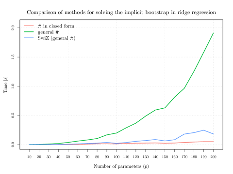
Figure 1: Average time in seconds (taken over 10 optimizations) for solving the implicit bootstrap in a ridge regression model of dimension $p$. Regression coefficients and the matrix of design are randomly generated from a standard normal distribution. The numerical methods using the closed form expression of $\widehat{{\bm{\pi}}}^{\ast}_{n}({\bm{\theta}})$ is in red ($\widehat{{\bm{\pi}}}$ in closed form), it has the lowest computational times. The numerical method based on the SwiZ is in blue (SwiZ (general $\widehat{{\bm{\pi}}}$)), it has a similar computational times. The numerical method ignoring the explicit form of $\widehat{{\bm{\pi}}}^{\ast}_{n}({\bm{\theta}})$ is in green (general $\widehat{{\bm{\pi}}}$), it has the highest computational times. We use the same C++ implementation of the L-BFGS algorithm as the optimization routine for all the methods.

4 Simulation study

In this section, we provide empirical evidences of the coverage accuracy and the implementation simplicity of the implicit bootstrap in two complex parametric scenarios. First, we consider in Section 4.1 a regression model where data is subject to censoring. In particular, we consider the Student regression when the response variable is censored, a case for which an EM algorithm has already been developed (Arellano-Valle et al., 2012). Second, we consider a heavy-tailed distribution, the Lomax distribution, in the potential presence of outliers that is dealt with, as argued in Section 4.2, by using a robust estimator.

In the main part of the paper we report the empirical coverage of the upper endpoints of one-sided intervals with $\alpha\in(0.9,1)$. The empirical coverage for the lower endpoints, i.e., $\alpha\in(0,0.1)$, are reported in Appendix C. We compare the implicit bootstrap, the parametric percentile bootstrap and the CIs based on asymptotic theory. When it is not too prohibitive computationally, we also include other bootstrap schemes. Overall the implicit bootstrap is the method that provides the most accurate coverage. Other methods can be highly unreliable, especially for relatively small sample sizes, thereby reinforcing the theoretical idea that the implicit bootstrap is second-order accurate in complex parametric problems. Moreover, as we use a simple inconsistent estimator as initial estimator in both cases, this shows that the implicit bootstrap is readily available for a large number of complex parametric models.

4.1 Student-t censored regression model

An extension to the linear regression model is to consider that the error distribution is more general than the Gaussian distribution in order to accommodate potential heavy tails, or even skewed distributions. This modelling approach can be seen as a way to provide robust estimators for the regression parameters (see e.g., He et al., 2000; He and Cui, 2004; Azzalini and Genton, 2008, and the references therein). We consider here the case of i.i.d. Student distributed errors, which is different than multivariate Student errors (see Lange et al., 1989, and the references therein), and which is a proper modelling to characterize heavy tails (see Breusch et al., 1997). Namely, the Student linear regression model, for responses $Y_{i},i=1,\ldots,n$ and associated covariates (including an intercept) ${\bf x}_{i}=[x_{ij}]_{j=0,\ldots,p}$, can be written as

$$Y_{i}={\bf x}_{i}^{\top}{\bm{\beta}}+\sigma\varepsilon_{i},\quad i=1,\dots,n,$$ (16)

where ${\bm{\beta}}=(\beta_{0}\;\beta_{1}\;\ldots\;\beta_{p})^{\top}$ and $\varepsilon_{i}\sim S_{\nu}$, the Student distribution with $\nu$ degrees of freedom.

Moreover, as argued in Arellano-Valle et al. (2012), one often observes a response variable whose support is limited, typically only positive values, which can be modelled as a censoring feature. For example, they consider the case of married women whose average hourly earnings (wage rates) were recorded together with a set of covariates. The wage rates were considered as censored for women who did not work the year the survey took place. As proposed in Arellano-Valle et al. (2012), one supposes that instead of observing $Y_{0}$ with conditional distribution in (16), one observes a subset $Y=Y_{0}\,\iota(Y_{0}\geq a)$ of size $n_{1}$, with $\iota(\cdot)$ the indicator function. Then, supposing that the censored proportion $n_{0}/n$, $n=n_{0}+n_{1}$, is known together with the covariates for the censored responses, and letting $d_{i}=\iota(y_{i}\geq a)$, the likelihood function is

$$L({\bm{\theta}})=\prod_{i=1}^{n}\left(\frac{1}{1-S_{\nu}\left(\frac{{\bf x}_{i}^{\top}{\bm{\beta}}-a}{\sigma}\right)}\right)^{1-d_{i}}\left(\frac{1}{\sigma}s_{\nu}\left(\frac{y_{i}-{\bf x}_{i}^{\top}{\bm{\beta}}}{\sigma}\right)\right)^{d_{i}}$$

where ${\bm{\theta}}$ is the vector formed by ${\bm{\beta}}$, $\sigma$ and the degrees of freedom $\nu$, and $S_{\nu}$ and $s_{\nu}$ are, respectively, the Student cumulative probability function and its density. To compute the MLE, Arellano-Valle et al. (2012) propose to use the EM algorithm and therefore develop the conditional (on $Y_{i}\geq a$, for $a=0$) expectations and variances. Garay et al. (2017) (with R package SMNCensReg of Garay et al., 2022) extend the EM for censored data to other types of distributions. Inference for the model’s parameters can be performed using the asymptotic covariance matrix by plugging in the parameters’ estimates (obtained from SMNCensReg), or perform a parametric bootstrap with the percentile method, again, using the MLE obtained from SMNCensReg. The studentized bootstrap is computationally prohibitive since the EM algorithm to compute the MLE is itself quite numerically involving.

In this simulation study, we instead propose to use the implicit bootstrap, with, as initial estimator, the MLE of the Student regression model in (16) ignoring the censoring mechanism, which is clearly an inconsistent estimator for the censored Student regression model’s parameters. Then, to compute $\widecheck{\bm{\theta}}_{n}^{\ast}$ in (1), the $b$th sample, $b=1,\ldots,B$, ${\bf Y}^{*}({\bm{\theta}})$ is simulated from the non censored model (16) and the simulated responses are censored at ${\bf Y}^{*}({\bm{\theta}})\geq a$ to compute $\widehat{{\bm{\pi}}}_{n}^{*}({\bm{\theta}})$, i.e. the MLE ignoring the censoring mechanism. We compare the coverage for one-sided CIs at different confidence levels $\alpha$, of the implicit bootstrap with the inconsistent initial estimator and the parametric percentile bootstrap on the MLE estimates computed using the SMNCensReg package, by means of a simulation study. We also consider, as a benchmark, the CIs obtained using the estimated asymptotic covariance matrix, readily available from SMNCensReg.

The simulation setting is based on the application on housewives average hourly earnings modelled in Arellano-Valle et al. (2012) and Garay et al. (2017) by using a left-censored (at $a=0$) Student regression. The original data described in Mroz (1987) consists of 753 married white women with ages ranging between 30 to 60 years in 1975. There is a total of fifteen available covariates, of which four were considered in Arellano-Valle et al. (2012) and Garay et al. (2017): the housewives’ age, their years of schooling, the number of children younger than six years old in the household and the number of children with ages ranging between 6 to 19 years. In the simulation study, we consider the full dataset but we set the slope coefficients to zero for the covariates other than the four selected ones. For the later, we set $\beta_{1}=-1,\beta_{2}=1.5,\beta_{3}=-0.5,\beta_{4}=-1.5$, $\sigma^{2}=2$, for the error variance and $\nu=2$, for the degrees of freedom. The covariates are centered and scaled, so that the conditional response expectation is a function of the intercept. We choose three values for the intercept to vary the percentage of censoring. Namely, with $\beta_{0}=2$, there is $20\%$ of censoring, with $\beta_{0}=4$, $10\%$ and with $\beta_{0}=6$, $5\%$. We consider three sample sizes: $n=100$, $n=200$ and $n=400$, and randomly subsample from the full design matrix to create the designs for these particular sample sizes. For each case, we simulate $10,000$ response variables of size $n$. The bootstrap distributions for all methods are obtained using $B=1,000$ bootstrap samples.

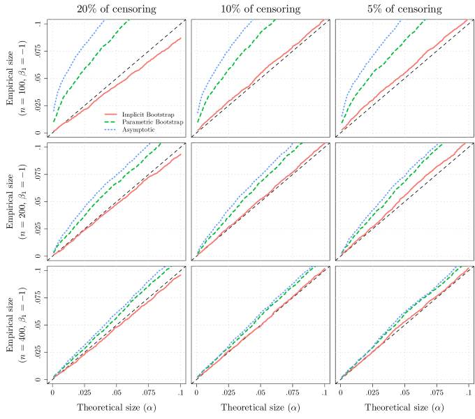
Figure 4: Coverage as a function of the confidence levels $\alpha\in(0\%,10\%)$ of CIs for $\beta_{1}=-1.0$. The simulation setting is the Student regression model with censored data at $a=0$. The coverage are computed using (in red solid line) the implicit bootstrap (based on the MLE ignoring the censoring mechanism) with $B=1,000$ simulated samples, (in green dashed line) the percentile parametric bootstrap based on the consistent MLE $B=1,000$ simulated samples and (in blue dotted line) the asymptotic method. The percentage of censoring is respectively 20% (first column), 10% (second column) and 5% (third column). The sample sizes are $n=100$ (first row), $n=200$ (second row) and $n=400$ (third row). We used $M=10,000$ Monte Carlo replicates.

In Figure 2 the performance of the implicit bootstrap (based on the MLE ignoring the censoring mechanism), the percentile parametric bootstrap based on the consistent MLE and the asymptotic method are compared using the coverage obtained by simulation. We consider only the confidence levels $\alpha\in(90\%,100\%)$ (see Figure 4 in Appendix C for $\alpha\in(0\%,10\%)$) as they are the most used ones and the CIs are computed for the parameter $\beta_{1}=-1.0$. For other parameters, the results are similar.

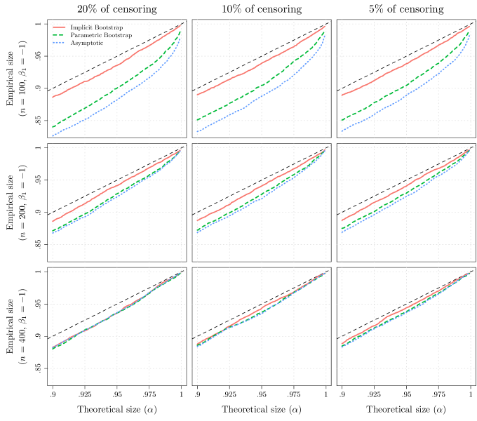
Figure 2: Coverage as a function of the confidence levels $\alpha\in(90\%,100\%)$ of CIs for $\beta_{1}=-1.0$. The simulation setting is the Student regression model with censored data at $a=0$. The coverage are computed using (in red solid line) the implicit bootstrap (based on the MLE ignoring the censoring mechanism) with $B=1,000$ simulated samples, (in green dashed line) the percentile parametric bootstrap based on the consistent MLE $B=1,000$ simulated samples and (in blue dotted line) the asymptotic method. The percentage of censoring is respectively 20% (first column), 10% (second column) and 5% (third column). The sample sizes are $n=100$ (first row), $n=200$ (second row) and $n=400$ (third row). We used $M=10,000$ Monte Carlo replicates.

The censoring proportion appears to affect essentially the performance of the implicit bootstrap which is slightly conservative with 20% censoring, but quite accurate with smaller censoring proportions. With all censoring proportions the percentile parametric bootstrap and the asymptotic method provide liberal coverage, with the asymptotic method being the most liberal, with a larger difference from the confidence level $\alpha$, compared to the implicit bootstrap. This difference is, as expected, reduced with larger sample sizes. To be more precise, considering 10% of censoring with $n=100$, at the confidence level of 95%, the coverage for the implicit bootstrap is of 93.9%, while it is of 90.5% for the percentile parametric bootstrap and of 88.8% for the asymptotic method. With $n=200$, these coverage are of 94.1% for the implicit bootstrap, 92.8% for the percentile parametric bootstrap and 92.1% for the asymptotic method. The simulation study hence confirms the theoretical advantages of the implicit bootstrap in terms of inferential accuracy, given that its accuracy is mostly very high and superior to the alternative methods when it is less accurate.

4.2 Heavy-tail density estimation

As an heavy-tail density, we consider here the popular Lomax distribution (Lomax, 1954) that is frequently used in business, economics, actuarial science, queueing theory, internet traffic modeling (see e.g., Holland et al., 2006), human dynamics (see e.g., Barabàsi, 2005). The Lomax distribution belongs to the family of Pareto distributions. It is essentially a Pareto distribution that has been shifted so that the lower bound of its support is 0. It is also often used to fit upper tails of distributions, where data are sparse, from which quantities such as probabilities associated with extreme events or risk measures are deduced (see e.g., Embrechts et al., 1997). It can also be used for estimating inequality measures or Lorenz curves (see e.g., Cowell and Victoria-Feser, 2007a).

The density function can be written as

$$\frac{q}{b}\left(1+\frac{y}{b}\right)^{-(q+1)},\quad y>0,$$

where $b>0$, $q>0$. The value of $q$ defines the existence of moments of this distribution, that is for $m\in\mathbb{N}^{\ast}$, $\mathbb{E}[X^{m}]$ is defined if $q>m$. However, in practice, small values for $q$ are possible; for example Holland et al. (2006) reported practical values to be in the range $(0.5,3.3)$. Moreover, it is known that the MLE for the Lomax parameters can be severely biased (see e.g., Giles et al., 2013, and the references therein), especially for values $q\leq 2$ for which the second moment does not exist, so that inference might provide very poor coverage. In addition, some authors have shown concern about the non-robustness of statistics computed from fitted Pareto distributions used in risk theory for insurance or finance, as well as for inequality measures; see e.g., Peng and Welsh (2001), Cowell and Victoria-Feser (2002), Brazauskas (2003), Dupuis and Field (2004), Dupuis and Victoria-Feser (2006), Cowell and Victoria-Feser (2007b) and Alfons et al. (2012). Hence, instead of the classical MLE, robust estimators have been used to estimate the model’s parameters, such a the Weighted MLE (WMLE) proposed by Field and Smith (1994). For the Lomax distribution, the likelihood score function is given by

$$s_{b}(y;{\bm{\theta}}) = (q+1)\frac{y}{b^{2}+by}-\frac{1}{b},$$

$$s_{q}(y;{\bm{\theta}}) = \frac{1}{q}-\hbox{log}\left(1+\frac{y}{b}\right),$$

and, letting $\mathbf{s}(y;{\bm{\theta}})=[s_{b}(y;{\bm{\theta}})\;\;s_{q}(y;{\bm{\theta}})]^{\top}$, the WMLE is simply obtained as the solution in ${\bm{\theta}}$ of

$$\sum_{i=1}^{n}w(y_{i};{\bm{\theta}})\mathbf{s}(y_{i};{\bm{\theta}})=\bm{0},$$ (17)

with, for the weight function $w$, an appropriate robust choice such as Huber’s weights (see e.g., Hampel et al., 1986). The WMLE in (17) with Huber’s weights is not consistent at the Lomax model, so that one considers replacing the right handside of (17) with a Fisher consistency correction factor which is defined by $\mathbb{E}\left[w(Y;{\bm{\theta}})\mathbf{s}(Y;{\bm{\theta}})\right]$, where the expectation is taken under the Lomax distribution. This correction factor does not admit a closed form so that numerical approximations are needed. Alternatively, Moustaki and Victoria-Feser (2006) propose to adjust for consistency a robust estimator using the principle of indirect inference. We use this approach to compute a Consistent WMLE (CWMLE) as a benchmark to the WMLE without consistency correction. Indeed, since our proposed inferential method does not need a consistent estimator, we also consider the later as initial estimator to compute (one-sided) CIs by means of the implicit bootstrap and compare the coverage with the percentile parametric bootstrap using the CWMLE. In addition, we also compute CIs based on the MLE using the implicit bootstrap, the percentile parametric bootstrap, the studentized parametric bootstrap and the BC${}_{\text{a}}$ parametric bootstrap (Efron, 1987).

The simulation study is based on $M=10,000$ synthetic samples of size $n$ drawn from the Lomax distribution with parameters set to the values $b=1$ and $q=1.5$. We consider three sample sizes $n=50$, $n=100$ and $n=200$ and choose $B=1,000$ bootstrap samples for each method. We compare the coverage of CIs using the different methods for the parameters of the Lomax distribution. Moreover, since the later is often used to estimate functions of the parameters, as for example the survival function $\vartheta(y)=(1+y/b)^{-q}$, used to model business failure (Lomax, 1954), we also compute the coverage of the later at a fixed value for $y$. In that case, we avoid using the studentized bootstrap or BC${}_{\text{a}}$ since they are not transformation respecting.

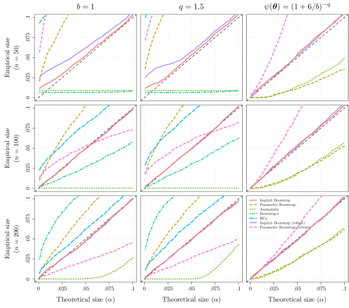
Figure 5: Coverage as a function of the confidence levels $\alpha\in(0\%,10\%)$ of CIs for $b=1$ (first column), $q=1.5$ (second column) and $\vartheta=(1+6/b)^{-q}$ (third column). The sample sizes are $n=50$ (first row), $n=100$ (second row) and $n=200$ (third row). Based on the MLE, the coverage probabilities are computed using (in red solid line) the implicit bootstrap, (in gold dashed line) the percentile parametric bootstrap, (in green dotted line) the asymptotic method, (in dark green dotdashed line) the studentized parametric bootstrap and (in blue dashed line) the BC${}_{\text{a}}$ parametric bootstrap. Based on the (inconsistent) WMLE, the coverage are computed using (in purple solid line) the implicit bootstrap and for the CWMLE (in pink dashed line) using the percentile parametric bootstrap. We used $M=10,000$ Monte Carlo replicates and $B=1,000$ bootstrap samples in all settings across all methods.

In Figure 3, the performance of the implicit bootstrap, the percentile parametric bootstrap as well as, when possible, the studentized parametric bootstrap and the BC${}_{\text{a}}$ parametric bootstrap are compared using the coverage obtained by simulation. The last two methods are not used for CIs of $\vartheta(y)$ since they are not transformation respecting, and also not for the CWMLE since the computational time is too prohibitive. Again, we consider only the confidence levels $\alpha\in(90\%,100\%)$ and for $\alpha\in(0\%,10\%)$, the results are presented in Figure 5 in Appendix C. The CIs for the parameters of the Lomax distribution based on the MLE have a seemingly exact coverage only with the implicit bootstrap. The other methods provide rather conservative CIs, especially for $n=50$ and $n=100$, while the coverage become more accurate when $n=200$, with the studentized parametric bootstrap being the most accurate. The comparison of the implicit bootstrap with the (inconsistent) WMLE and the percentile parametric bootstrap with the CWMLE, shows that the CIs with the former are seemingly exact while they are very liberal for the later. This later results perfectly highlights the advantages of the implicit bootstrap, not only because of its finite sample properties, but also because it can be based on an inconsistent estimator without apparent loss of accuracy. Moreover, based on our implementation, it was on average 1200 faster to compute the implicit bootstrap distribution. The comparison of coverage for the CIs for $\vartheta(y)$ using the implicit bootstrap and the percentile parametric bootstrap based on the MLE leads to a similar conclusion, that is the the later produces very liberal coverage, while the former is seemingly exact for $n=100$ and $n=200$, while for $n=50$ it produces slightly liberal CIs. Finally, the same conclusion can be drawn when comparing the implicit bootstrap with the WMLE and the percentile bootstrap with the CWMLE.

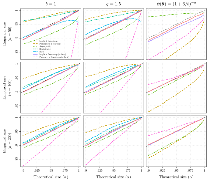
Figure 3: Coverage as a function of the confidence levels $\alpha\in(90\%,100\%)$ of CIs for $b=1$ (first column), $q=1.5$ (second column) and $\vartheta=(1+6/b)^{-q}$ (third column). The sample sizes are $n=50$ (first row), $n=100$ (second row) and $n=200$ (third row). Based on the MLE, the coverage probabilities are computed using (in red solid line) the implicit bootstrap, (in gold dashed line) the percentile parametric bootstrap, (in green dotted line) the asymptotic method, (in dark green dotdashed line) the studentized parametric bootstrap and (in blue dashed line) the BC${}_{\text{a}}$ parametric bootstrap. Based on the (inconsistent) WMLE, the coverage are computed using (in purple solid line) the implicit bootstrap and for the CWMLE (in pink dashed line) using the percentile parametric bootstrap. We used $M=10,000$ Monte Carlo replicates and $B=1,000$ bootstrap samples in all settings across all methods.

Appendix A Related Methods

When simulated data can easily be generated for any parameter value, it is natural to consider indirect inference methods (see e.g., Smith, 1993; Gouriéroux et al., 1993; Gallant and Tauchen, 1996; Guerrier et al., 2019; Zhang et al., 2023) to obtain consistent estimators out of possibly inconsistent ones. Using our notations, an indirect estimator, in the just identified case, can be defined as follows

$$\widehat{\bm{\theta}}^{\ast}_{n,H}=\operatorname*{argzero}_{{\bm{\theta}}\in{\bm{\Theta}}}\widehat{{\bm{\pi}}}_{n}({\bm{\theta}}_{0})-\frac{1}{H}\sum^{H}_{h=1}\widehat{{\bm{\pi}}}_{n,h}^{\ast}({\bm{\theta}}),$$ (A1)

where $H\geq 1$ and $\widehat{{\bm{\pi}}}_{n,h}^{\ast}({\bm{\theta}})$ is computed on the simulated sample ${\bf Y}_{h}^{\ast}({\bm{\theta}})$ for $h=1,\dots,H$. The left term of the left hand-side of (A1) is an estimator of ${\bm{\pi}}({\bm{\theta}})$, the non-stochastic limit of $\widehat{{\bm{\pi}}}_{n}({\bm{\theta}})$, and therefore, $H$ should be large enough. The implicit bootstrap estimator corresponds to the indirect inference estimator in the just identified case with $H=1$, i.e. $\widecheck{\bm{\theta}}^{\ast}_{n}=\widehat{\bm{\theta}}^{\ast}_{n,1}$. When $H=\infty$ in (A1), we get the Just Identified Indirect Inference (JINI) estimator defined in Zhang et al. (2023), denoted here as $\widehat{\bm{\theta}}_{n,\infty}$.

Both $\widehat{\bm{\theta}}^{\ast}_{n,H}$ and $\widehat{\bm{\theta}}_{n,\infty}$ provide good point estimates for ${\bm{\theta}}_{0}$ (see Guerrier et al., 2019; Zhang et al., 2023), however, CIs based on either one estimator may still be computationally burdensome to construct. Indeed, on the one hand, estimating the covariance matrix (analytically or by bootstrap) involves the Jacobian $\bm{A}({\bm{\theta}})\vcentcolon=\partial{\bm{\pi}}({\bm{\theta}})/\partial{\bm{\theta}}^{\top}$ of the unknown function ${\bm{\pi}}({\bm{\theta}})$, and on the other hand, computing the bootstrapped JINI $\widehat{{\bm{\theta}}}_{n,\infty}^{\ast}$ or indirect inference estimator $\widehat{{\bm{\theta}}}_{n,H}^{\ast}$, is computationally very intensive. Approximations for $\bm{A}({\bm{\theta}})$ have been put forward by e.g., Genton and De Luna (2000) who propose to use a numerical approximations, by Gouriéroux and Monfort (1996) who propose an approximation of $\bm{A}$ when the objective function determining $\widehat{{\bm{\pi}}}_{n}$ is smooth, idea that has been also used in Genton and Ronchetti (2003) and Moustaki and Victoria-Feser (2006) when $\widehat{{\bm{\pi}}}_{n}$ is a M-estimator, and by Armstrong et al. (2014) in the context of generalized method of moment estimators. Alternatively, one may try to alleviate the numerical problem by the use of faster bootstrap alternatives, although at the price of accuracy in finite sample (see e.g., Honoré and Hu, 2017, and references therein). On the other hand, the implicit bootstrap not only solely rely on the (theoretical) existence of the implicit estimator, thereby greatly lessening the computational cost, but also provides guarantees for higher-order properties such as second-order accurate CIs.

The implicit bootstrap also shares some similarities with generalized fiducial inference (Hannig et al., 2016). Indeed, the later also relies on a matching criterion, but on a summary or sufficient statistic of the data, from which a distribution is derived, namely the generalized fiducial distribution, which is used to construct CIs. Using our notations the later, for ${\bm{\theta}}_{0}$, is obtained by solving

$$~{}{\bm{\theta}}_{n}^{\ast}\vcentcolon=\operatorname*{argzero}_{{\bm{\theta}}\in{\bm{\Theta}}}\bm{s}\{{\bf Y}({\bm{\theta}}_{0})\}-\bm{s}\{{\bf Y}^{\ast}({\bm{\theta}})\},$$ (A2)

where $\bm{s}\{{\bf Y}({\bm{\theta}})\}$ is the summary or sufficient statistic, for any ${\bm{\theta}}\in{\bm{\Theta}}$. In the special case where $\bm{s}\{{\bf Y}({\bm{\theta}}_{0})\}$ is an estimator of ${\bm{\theta}}_{0}$, the implicit bootstrap distribution and the generalized fiducial distribution coincide, so that the implicit bootstrap can be considered as a special case of the very broad generalized fiducial inference framework. However, when $\bm{s}\{{\bf Y}({\bm{\theta}}_{0})\}$ is not an estimator of ${\bm{\theta}}_{0}$ (i.e. the implicit bootstrap), it is well known that obtaining the generalized fiducial distribution can be very difficult, due to the almost impossibility of solving (A2) directly, or due the fact that finding appropriate summary or sufficient statistic can be very challenging (see e.g., Hannig et al., 2014, 2016). This particular problem is shared with another related method, namely the ABC method, see e.g., Beaumont et al. (2002); Robert (2007); Beaumont (2010); Fearnhead and Prangle (2012); Robert (2016). In contrast, our approach allows more flexibility in that the matching criterion, through the choice of the initial estimator, can be chosen for its simplicity.

Appendix B Proofs

Throughout this section, we will assume that all the random elements we consider (variables, vectors or matrices) correspond to ^q-valued Borel mesurable maps, where $q\in\mathbb{N}$ may depend on the context. Also, we use the notation $\forall^{\infty}$ to say ”for almost all”.

B.1 Proof of 1

We will use two Lemmas in order to show 1. The first one is a uniform Skorokhod’s representation theorem.

Lemma 2:

Under 3, let ${\bf X}_{n}({\bm{\theta}})\vcentcolon=a_{n}{\bf\Sigma}_{n}({\bm{\theta}})^{-\nicefrac{{1}}{{2}}}\{\widehat{{\bm{\pi}}}_{n}({\bm{\theta}})-{\bm{\pi}}({\bm{\theta}})\}$, for each ${\bm{\theta}}\in{\bm{\Theta}}_{1}$. Then, there exists, for each ${\bm{\theta}}\in{\bm{\Theta}}_{1}$, a random sequence $\widetilde{{\bf X}}_{n}({\bm{\theta}})$ such that

1. $\widetilde{{\bf X}}_{n}({\bm{\theta}})\overset{\text{a.s.}}{\longrightarrow}{\bf Z}$ uniformly in ${\bm{\theta}}\in{\bm{\Theta}}_{1}$,

2. $\widetilde{{\bf X}}_{n}({\bm{\theta}})\overset{d}{=}{\bf X}_{n}({\bm{\theta}})$, for each $n\in\mathbb{N}$ and each ${\bm{\theta}}\in{\bm{\Theta}}_{1}$.

This uniform version of Skorokhod’s representation theorem can be deduced from a generalized Skorokhod’s representation theorem proved in Van Der Vaart and Wellner, 1996.

Proof of 2.

We consider the pair $(\mathcal{A},\leqslant_{l})$, where $\mathcal{A}\vcentcolon=\mathbb{N}\times{\bm{\Theta}}_{1}$ and $\leqslant_{l}$ denotes the lexicographic order, making $\mathcal{A}$ a directed set. This allows us to consider convergence indexed by elements of $\mathcal{A}$. Namely, identifying ${\bf X}_{\mathfrak{a}}$ to ${\bf X}_{n}({\bm{\theta}})$ for $\mathfrak{a}=(n,{\bm{\theta}})\in\mathcal{A}$ and denoting $F_{\mathfrak{a}}$ and $F$ the cumulative distribution functions of ${\bf X}_{\mathfrak{a}}$ and ${\bf Z}$ respectively, we have

$${\bf X}_{\mathfrak{a}}\buildrel d\over{\longrightarrow}{\bf Z}\quad\text{if and only if}\quad\forall\varepsilon>0,\exists\,\mathfrak{a}_{\varepsilon}\in\mathcal{A},\forall\mathfrak{a}\geqslant\mathfrak{a}_{\varepsilon},\;\sup_{x}|F_{\mathfrak{a}}(x)-F(x)|<\varepsilon.$$

Similarly, assuming there is a common sample space ${\bm{\Omega}}$ corresponding to every (Borel measurable map) ${\bf X}_{\mathfrak{a}}$, we have

$${\bf X}_{\mathfrak{a}}\buildrel a.s.\over{\longrightarrow}{\bf Z}\quad\text{if and only if}\quad\forall^{\infty}\bm{\omega}\in{\bm{\Omega}},\forall\varepsilon>0,\exists\,\mathfrak{a}_{\varepsilon,\bm{\omega}}\in\mathcal{A},\forall\mathfrak{a}\geqslant\mathfrak{a}_{\varepsilon,\bm{\omega}},\;\|{\bf X}_{\mathfrak{a}}(\bm{\omega})-{\bf Z}(\bm{\omega})\|<\varepsilon.$$

Thus, it is easy show that

• ${\bf X}_{n}({\bm{\theta}})\buildrel d\over{\longrightarrow}{\bf Z}$ uniformly in ${\bm{\theta}}\in{\bm{\Theta}}_{1}$ if and only if ${\bf X}_{\mathfrak{a}}\buildrel d\over{\longrightarrow}{\bf Z}$,

• ${\bf X}_{n}({\bm{\theta}})\buildrel a.s.\over{\longrightarrow}{\bf Z}$ uniformly in ${\bm{\theta}}\in{\bm{\Theta}}_{1}$ if and only if ${\bf X}_{\mathfrak{a}}\buildrel a.s.\over{\longrightarrow}{\bf Z}$.

Since all the random elements we consider correspond to ^p-valued Borel mesurable maps, we can use Lemmas 1.9.2, 1.9.6 and Theorem 1.10.3 of Van Der Vaart and Wellner, 1996 to conclude the proof. ∎

An important consequence of 2, is that it allows us to consider, without loss of generality, a common sample space ${\bm{\Omega}}\subset{}^{m}$ for the entire family of random vectors $\{\widehat{{\bm{\pi}}}_{n}({\bm{\theta}})\}_{n\in\mathbb{N},{\bm{\theta}}\in{\bm{\Theta}}_{1}}$. In other words, for any $n\in\mathbb{N}$ and any ${\bm{\theta}}\in{\bm{\Theta}}_{1}$, the estimator $\widehat{{\bm{\pi}}}_{n}({\bm{\theta}})$, as well as its simulated versions $\widehat{{\bm{\pi}}}_{n}^{\ast}({\bm{\theta}})$ and $\widehat{{\bm{\pi}}}_{n}^{\ast\ast}({\bm{\theta}})$, can be thought of as the function

$$\begin{array}[]{rccl}\widehat{{\bm{\pi}}}_{n}:&{\bm{\Theta}}_{1}\times{\bm{\Omega}}&\to&{}^{p}\\ &({\bm{\theta}},\bm{\omega})&\mapsto&\widehat{{\bm{\pi}}}_{n}({\bm{\theta}},\bm{\omega})\end{array}$$

Similarly, the implicit estimator $\widehat{\bm{\theta}}_{n}={\bm{\pi}}^{-1}\{\widehat{{\bm{\pi}}}_{n}({\bm{\theta}}_{0})\}$ can also be thought as a function $\widehat{\bm{\theta}}_{n}\vcentcolon={\bm{\pi}}^{-1}\circ\widehat{{\bm{\pi}}}_{n}({\bm{\theta}}_{0},\cdot)$, where $\widehat{{\bm{\pi}}}_{n}({\bm{\theta}}_{0},\cdot):{\bm{\Omega}}\to{}^{p}$. Consequently, Eq. 1 can be written, for almost all $\bm{\omega},\bm{\omega}^{\ast}\in{\bm{\Omega}}$, as follows

$$\widecheck{\bm{\theta}}_{n}(\bm{\omega},\bm{\omega}^{\ast})\in\operatorname*{argmin}_{{\bm{\theta}}\in{\bm{\Theta}}}\;\|\widehat{{\bm{\pi}}}_{n}({\bm{\theta}}_{0},\bm{\omega})-\widehat{{\bm{\pi}}}_{n}({\bm{\theta}},\bm{\omega}^{\ast})\|,$$

so that the implicit bootstrap estimator is thought as a function $\widecheck{\bm{\theta}}_{n}:{\bm{\Omega}}^{2}\to{}^{p}$. Notice that Eq. 2 implies this latter definition.

The second and third lemmas characterize the limiting distribution of $\widecheck{\bm{\theta}}_{n}^{\ast}$.

Lemma 3:

Under Assumptions 1, 2 and 3, and conditionally on the implicit estimator $\widehat{\bm{\theta}}_{n}={\bm{\pi}}^{-1}\{\widehat{{\bm{\pi}}}_{n}({\bm{\theta}}_{0})\}$, we have that, $\widecheck{\bm{\theta}}_{n}^{\ast}=\widehat{\bm{\theta}}_{n}+o_{p}(1)$, in probability.

Proof of 3.

Using 2, we can assume that ${\bf X}_{n}({\bm{\theta}})\overset{\text{a.s.}}{\longrightarrow}{\bf Z}$ uniformly in ${\bm{\theta}}\in{\bm{\Theta}}_{1}$, where ${\bf X}_{n}({\bm{\theta}})=a_{n}{\bf\Sigma}_{n}({\bm{\theta}})^{-\nicefrac{{1}}{{2}}}\{\widehat{{\bm{\pi}}}_{n}({\bm{\theta}})-{\bm{\pi}}({\bm{\theta}})\}$. Therefore, letting ${\bm{\Omega}}$ be the common sample space of the random vectors ${\bf X}_{n}({\bm{\theta}})$ and ${\bf Z}$, we have $\forall^{\infty}$ $\bm{\omega}\in{\bm{\Omega}}$ and uniformly in ${\bm{\theta}}\in{\bm{\Theta}}_{1}$, ${\bf X}_{n}({\bm{\theta}},\bm{\omega})={\bf Z}(\bm{\omega})+o(1)$. The latter equality can be written as follows,

$$\widehat{{\bm{\pi}}}_{n}({\bm{\theta}},\bm{\omega})={\bm{\pi}}({\bm{\theta}})+a_{n}^{-1}{\bf\Sigma}_{n}({\bm{\theta}})^{\nicefrac{{1}}{{2}}}{\bf Z}(\bm{\omega})+o(a_{n}^{-1}),$$

$\forall^{\infty}$ $\bm{\omega}\in{\bm{\Omega}}$ and uniformly in ${\bm{\theta}}\in{\bm{\Theta}}_{1}$. By 3, ${\bf\Sigma}_{n}({\bm{\theta}})$ can replaced by its limit ${\bf\Sigma}({\bm{\theta}})$ so that we have $\forall^{\infty}$ $\bm{\omega}\in{\bm{\Omega}}$ and uniformly in ${\bm{\theta}}\in{\bm{\Theta}}_{1}$,

$$~{}\widehat{{\bm{\pi}}}_{n}({\bm{\theta}},\bm{\omega})={\bm{\pi}}({\bm{\theta}})+a_{n}^{-1}{\bf\Sigma}({\bm{\theta}})^{\nicefrac{{1}}{{2}}}{\bf Z}(\bm{\omega})+o(a_{n}^{-1}).$$ (B1)

Hence, since ${\bm{\Theta}}_{1}$ is compact and ${\bf\Sigma}({\bm{\theta}})$ is continuous by Assumptions 1 and 3 respectively, we have $\forall^{\infty}$ $\bm{\omega}\in{\bm{\Omega}}$ and uniformly in ${\bm{\theta}}\in{\bm{\Theta}}_{1}$,

$$~{}\widehat{{\bm{\pi}}}_{n}({\bm{\theta}},\bm{\omega})={\bm{\pi}}({\bm{\theta}})+\mathcal{O}(a_{n}^{-1}).$$ (B2)

In particular, $\forall^{\infty}$ $\bm{\omega}\in{\bm{\Omega}}$ and for $n\in\mathbb{N}$ large enough, $\widehat{{\bm{\pi}}}_{n}({\bm{\theta}}_{0},\bm{\omega})\in{\bm{\pi}}({\bm{\Theta}}_{1})$. This implies that $\widehat{\bm{\theta}}_{n}(\bm{\omega})\in{\bm{\Theta}}_{1}$ $\forall^{\infty}$ $\bm{\omega}\in{\bm{\Omega}}$ and for $n\in\mathbb{N}$ large enough and, more precisely, that $\widehat{\bm{\theta}}_{n}(\bm{\omega})={\bm{\theta}}_{0}+o(1)$ $\forall^{\infty}$ $\bm{\omega}\in{\bm{\Omega}}$. Therefore, using Eq. B2, we have, $\forall^{\infty}$ $\bm{\omega},\bm{\omega}^{\ast}\in{\bm{\Omega}}$

$$~{}\widehat{{\bm{\pi}}}_{n}\{\widehat{\bm{\theta}}_{n}(\bm{\omega}),\bm{\omega}^{\ast}\}={\bm{\pi}}\{\widehat{\bm{\theta}}_{n}(\bm{\omega})\}+\mathcal{O}(a_{n}^{-1})=\widehat{{\bm{\pi}}}_{n}({\bm{\theta}}_{0},\bm{\omega})+\mathcal{O}(a_{n}^{-1}).$$ (B3)

The last equality and Eq. B2 imply that, $\forall^{\infty}$ $\bm{\omega},\bm{\omega}^{\ast}\in{\bm{\Omega}}$, a solution $\widecheck{\bm{\theta}}_{n}(\bm{\omega},\bm{\omega}^{\ast})\!\in\!{\bm{\Theta}}_{1}$ of

$$\operatorname*{argmin}_{{\bm{\theta}}\in{\bm{\Theta}}_{1}}\|\widehat{{\bm{\pi}}}_{n}({\bm{\theta}}_{0},\bm{\omega})-\widehat{{\bm{\pi}}}_{n}({\bm{\theta}},\bm{\omega}^{\ast})\|,$$

must satisfy

$$\widehat{{\bm{\pi}}}_{n}\{\widecheck{\bm{\theta}}_{n}(\bm{\omega},\bm{\omega}^{\ast}),\bm{\omega}^{\ast}\}\!=\!\widehat{{\bm{\pi}}}_{n}({\bm{\theta}}_{0},\bm{\omega})+\mathcal{O}(a_{n}^{-1})\quad\text{and}\quad\widehat{{\bm{\pi}}}_{n}\{\widecheck{\bm{\theta}}_{n}(\bm{\omega},\bm{\omega}^{\ast}),\bm{\omega}^{\ast}\}\!=\!{\bm{\pi}}\{\widecheck{\bm{\theta}}_{n}(\bm{\omega},\bm{\omega}^{\ast})\}+\mathcal{O}(a_{n}^{-1}).$$

From there and using Eq. B3, we deduce that $\forall^{\infty}$ $\bm{\omega},\bm{\omega}^{\ast}\in{\bm{\Omega}}$

$${\bm{\pi}}\{\widecheck{\bm{\theta}}_{n}(\bm{\omega},\bm{\omega}^{\ast})\}-{\bm{\pi}}\{\widehat{\bm{\theta}}_{n}(\bm{\omega})\}=\mathcal{O}(a_{n}^{-1}).$$

Hence, by 2, $\widecheck{\bm{\theta}}_{n}(\bm{\omega},\bm{\omega}^{\ast})={\bm{\pi}}^{-1}\left[{\bm{\pi}}\{\widehat{\bm{\theta}}_{n}(\bm{\omega})\}+o(1)\right]$, which implies

$$~{}\widecheck{\bm{\theta}}_{n}(\bm{\omega},\bm{\omega}^{\ast})-\widehat{\bm{\theta}}_{n}(\bm{\omega})=o(1),$$ (B4)

since ${\bm{\pi}}^{-1}$ is unifomly continuous on ${\bm{\Theta}}_{1}$, by Assumptions 1 and 2, and concludes the proof.

∎

Lemma 4:

Under Assumptions 1, 2 and 3, we have that, conditionally on the implicit estimator $\widehat{\bm{\theta}}_{n}={\bm{\pi}}^{-1}\{\widehat{{\bm{\pi}}}_{n}({\bm{\theta}}_{0})\}$,

$$a_{n}{\bf\Sigma}_{n}(\widehat{\bm{\theta}}_{n})^{-\nicefrac{{1}}{{2}}}\bm{A}(\widehat{\bm{\theta}}_{n})\left(\widecheck{\bm{\theta}}_{n}^{\ast}-\widehat{\bm{\theta}}_{n}\right)\buildrel d\over{\longrightarrow}-{\bf Z},\,\text{almost surely.}$$

Proof of 4.

Considering Eq. B1 in the proof of 3, and using the continuity of ${\bf\Sigma}({\bm{\theta}})$ and the fact that ${\bm{\Theta}}_{1}$ is compact by Assumptions 1 and 2, we have that $\forall^{\infty}$ $\bm{\omega},\bm{\omega}^{\ast}\in{\bm{\Omega}}$, and, for $n\in\mathbb{N}$ large enough, $\widehat{{\bm{\pi}}}_{n}({\bm{\theta}}_{0},\bm{\omega})-a_{n}^{-1}{\bf\Sigma}({\bm{\theta}}_{0})^{\nicefrac{{1}}{{2}}}{\bf Z}(\bm{\omega}^{\ast})\in{\bm{\pi}}({\bm{\Theta}}_{1})$. In other words, there exists $\bar{{\bm{\theta}}}_{n}(\bm{\omega},\bm{\omega}^{\ast})\in{\bm{\Theta}}_{1}$ such that, $\forall^{\infty}$ $\bm{\omega},\bm{\omega}^{\ast}\in{\bm{\Omega}}$ and $n\in\mathbb{N}$ large enough,

$${\bm{\pi}}\{\bar{\bm{\theta}}_{n}(\bm{\omega},\bm{\omega}^{\ast})\}=\widehat{{\bm{\pi}}}_{n}({\bm{\theta}}_{0},\bm{\omega})-a_{n}^{-1}{\bf\Sigma}({\bm{\theta}}_{0})^{\nicefrac{{1}}{{2}}}{\bf Z}(\bm{\omega}^{\ast}).$$

Moreover, by continuity of ${\bm{\pi}}^{-1}$, we deduce that $\bar{\bm{\theta}}_{n}(\bm{\omega},\bm{\omega}^{\ast})={\bm{\theta}}_{0}+o(1)$ $\forall^{\infty}$ $\bm{\omega},\bm{\omega}^{\ast}\in{\bm{\Omega}}$. Hence, using Eq. B1, the continuous mapping theorem and Assumptions 1 and 2 we deduce that $\forall^{\infty}$ $\bm{\omega},\bm{\omega}^{\ast}\in{\bm{\Omega}}$

$$\widehat{{\bm{\pi}}}_{n}\{\bar{\bm{\theta}}_{n}(\bm{\omega},\bm{\omega}^{\ast}),\bm{\omega}^{\ast}\} ={\bm{\pi}}\{\bar{\bm{\theta}}_{n}(\bm{\omega},\bm{\omega}^{\ast})\}+a_{n}^{-1}{\bf\Sigma}\{\bar{\bm{\theta}}_{n}(\bm{\omega},\bm{\omega}^{\ast})\}^{\nicefrac{{1}}{{2}}}{\bf Z}(\bm{\omega}^{\ast})+o(a_{n}^{-1})$$

$$={\bm{\pi}}\{\bar{\bm{\theta}}_{n}(\bm{\omega},\bm{\omega}^{\ast})\}+a_{n}^{-1}{\bf\Sigma}({\bm{\theta}}_{0})^{\nicefrac{{1}}{{2}}}{\bf Z}(\bm{\omega}^{\ast})+o(a_{n}^{-1})$$

$$=\widehat{{\bm{\pi}}}_{n}({\bm{\theta}}_{0},\bm{\omega})+o(a_{n}^{-1}).$$

The last equality and Eq. B1 imply that, $\forall^{\infty}$ $\bm{\omega},\bm{\omega}^{\ast}\in{\bm{\Omega}}$, a solution $\widecheck{\bm{\theta}}_{n}(\bm{\omega},\bm{\omega}^{\ast})\!\in\!{\bm{\Theta}}_{1}$ of

$$\operatorname*{argmin}_{{\bm{\theta}}\in{\bm{\Theta}}_{1}}\|\widehat{{\bm{\pi}}}_{n}({\bm{\theta}}_{0},\bm{\omega})-\widehat{{\bm{\pi}}}_{n}({\bm{\theta}},\bm{\omega}^{\ast})\|,$$

must satisfy

$$~{}\widehat{{\bm{\pi}}}_{n}\{\widecheck{\bm{\theta}}_{n}(\bm{\omega},\bm{\omega}^{\ast}),\bm{\omega}^{\ast}\}=\widehat{{\bm{\pi}}}_{n}({\bm{\theta}}_{0},\bm{\omega})+o(a_{n}^{-1})$$ (B5)

By Eq. B1 and (B4), we have

$$~{}\begin{split}\widehat{{\bm{\pi}}}_{n}\{\widecheck{\bm{\theta}}_{n}(\bm{\omega},\bm{\omega}^{\ast}),\bm{\omega}^{\ast}\}&={\bm{\pi}}\{\widecheck{\bm{\theta}}_{n}(\bm{\omega},\bm{\omega}^{\ast})\}+a_{n}^{-1}{\bf\Sigma}\{\widecheck{\bm{\theta}}_{n}(\bm{\omega},\bm{\omega}^{\ast})\}^{\nicefrac{{1}}{{2}}}{\bf Z}(\bm{\omega}^{\ast})+o(a_{n}^{-1})\\ &={\bm{\pi}}\{\widecheck{\bm{\theta}}_{n}(\bm{\omega},\bm{\omega}^{\ast})\}+a_{n}^{-1}{\bf\Sigma}\{\widehat{\bm{\theta}}_{n}(\bm{\omega})\}^{\nicefrac{{1}}{{2}}}{\bf Z}(\bm{\omega}^{\ast})+o(a_{n}^{-1}),\end{split}$$ (B6)

where the continuous mapping theorem is used in the second equality. Using Eq. B5 and (B6) and since ${\bm{\pi}}\{\widehat{\bm{\theta}}_{n}(\bm{\omega})\}=\widehat{{\bm{\pi}}}_{n}({\bm{\theta}}_{0},\bm{\omega})$ $\forall^{\infty}$ $\bm{\omega}\in{\bm{\Omega}}$, we can derive that, $\forall^{\infty}$ $\bm{\omega},\bm{\omega}^{\ast}\in{\bm{\Omega}}$,

$${\bm{\pi}}\{\widecheck{\bm{\theta}}_{n}(\bm{\omega},\bm{\omega}^{\ast})\}-{\bm{\pi}}\{\widehat{\bm{\theta}}_{n}(\bm{\omega})\}=-a_{n}^{-1}{\bf\Sigma}\{\widehat{\bm{\theta}}_{n}(\bm{\omega})\}^{\nicefrac{{1}}{{2}}}{\bf Z}(\bm{\omega}^{\ast})+o(a_{n}^{-1}).$$

Finally, 2, the mean value theorem and the continuous mapping theorem and to get, that $\forall^{\infty}$ $\bm{\omega},\bm{\omega}^{\ast}\in{\bm{\Omega}}$,

$$a_{n}{\bf\Sigma}\{\widehat{\bm{\theta}}_{n}(\bm{\omega})\}^{-\nicefrac{{1}}{{2}}}\bm{A}\{\widehat{\bm{\theta}}_{n}(\bm{\omega})\}\{\widecheck{\bm{\theta}}_{n}(\bm{\omega},\bm{\omega}^{\ast})-\widehat{\bm{\theta}}_{n}(\bm{\omega})\}=-{\bf Z}(\bm{\omega}^{\ast})+o(1),$$

leading to the result.∎

We now give the proof of 1.

Proof of 1.

From 4 and using the delta method, we have that

$$\hat{\xi}_{n}\vcentcolon=a_{n}\varsigma(\widehat{\bm{\theta}}_{n})^{-1}(\vartheta_{0}-\hat{\vartheta}_{n}) \buildrel d\over{\longrightarrow}\xi,$$

$$\check{\xi}_{n}^{\ast}\vcentcolon=a_{n}\varsigma(\widehat{\bm{\theta}}_{n})^{-1}(\check{\vartheta}^{\ast}_{n}-\hat{\vartheta}_{n}) \buildrel d\over{\longrightarrow}\xi,\,\text{almost surely},$$

where $\xi$ is a certain absolutely continuous random variable that does not depend on ${\bm{\theta}}\in{\bm{\Theta}}$ and $\varsigma({\bm{\theta}})=\frac{\partial\psi}{\partial{\bm{\theta}}}({\bm{\theta}})^{\top}\{\bm{A}({\bm{\theta}})^{-1}\}^{\top}{\bf\Sigma}({\bm{\theta}})\bm{A}({\bm{\theta}})^{-1}\frac{\partial\psi}{\partial{\bm{\theta}}}({\bm{\theta}})$ for ${\bm{\theta}}\in{\bm{\Theta}}_{1}$. From here, the arguments of the proof of Lemma 23.3 in Van der Vaart, 1998 apply and allow us to conclude that the $\alpha$-level quantile of $\check{\xi}_{n}^{\ast}$ converges almost surely to its correspond for $\xi$, i.e. $\check{\xi}_{n}^{\ast}(\alpha)\buildrel a.s.\over{\longrightarrow}\xi(\alpha)$. One can show that we have $\check{\xi}_{n}^{\ast}(\alpha)=a_{n}\varsigma(\widehat{\bm{\theta}}_{n})^{-1}\{\check{\vartheta}^{\ast}_{n}(\alpha)-\hat{\vartheta}_{n}\}$ and thus we have

$$\Pr\{\vartheta_{0}\leq\check{\vartheta}^{\ast}_{n}(\alpha)\} =\Pr\{\hat{\xi}_{n}\leq\check{\xi}_{n}^{\ast}(\alpha)\}=\Pr\{\xi\leq{\xi}(\alpha)\}+o(1)=\alpha+o(1),$$

concluding the proof.

∎

B.2 Proof of 2

In this subsection we give the proofs of 1, 1 and 2. We recall that all the random variables are absolutely continuous in this subsection.

Proof of 1.

Since Assumptions 4 and 5 imply Assumptions 2 and 3, we can use 2. More precisely, we can write that, $\forall^{\infty}\bm{\omega}\in{\bm{\Omega}}$

$$\widehat{{\bm{\pi}}}_{n}({\bm{\theta}},\bm{\omega})={\bm{\pi}}({\bm{\theta}})+n^{-\nicefrac{{1}}{{2}}}{\bf\Sigma}({\bm{\theta}})^{\nicefrac{{1}}{{2}}}{\bf Z}(\bm{\omega})+n^{-1}{\bf R}_{n}({\bm{\theta}},\bm{\omega})$$ (B7)

with ${\bf R}_{n}({\bm{\theta}},\bm{\omega})=\mathcal{O}(1)$, uniformly in ${\bm{\theta}}\in{\bm{\Theta}}_{1}$. Similarly to the proof of 4, we have that $\forall^{\infty},\bm{\omega},\bm{\omega}^{\ast}\in{\bm{\Omega}}$ and for $n\in\mathbb{N}$ large enough, there exists $\bar{{\bm{\theta}}}_{n}(\bm{\omega},\bm{\omega}^{\ast}),\widetilde{{\bm{\theta}}}_{n}(\bm{\omega},\bm{\omega}^{\ast})\in{\bm{\Theta}}_{1}$ such that

$${\bm{\pi}}\{\bar{\bm{\theta}}_{n}(\bm{\omega},\bm{\omega}^{\ast})\} =\widehat{{\bm{\pi}}}_{n}({\bm{\theta}}_{0},\bm{\omega})-n^{-\nicefrac{{1}}{{2}}}{\bf\Sigma}({\bm{\theta}}_{0})^{\nicefrac{{1}}{{2}}}{\bf Z}(\bm{\omega}^{\ast}),$$

$${\bm{\pi}}\{\widetilde{\bm{\theta}}_{n}(\bm{\omega},\bm{\omega}^{\ast})\} =\widehat{{\bm{\pi}}}_{n}({\bm{\theta}}_{0},\bm{\omega})-n^{-\nicefrac{{1}}{{2}}}{\bf\Sigma}\{\bar{\bm{\theta}}_{n}(\bm{\omega},\bm{\omega}^{\ast})\}^{\nicefrac{{1}}{{2}}}{\bf Z}(\bm{\omega}^{\ast})-n^{-1}{\bf R}_{n}\{\bar{\bm{\theta}}_{n}(\bm{\omega},\bm{\omega}^{\ast}),\bm{\omega}^{\ast}\}.$$

Since ${\bm{\pi}}^{-1}$ is continuously differentiable on the compact space ${\bm{\pi}}({\bm{\Theta}}_{1})$ from Assumptions 1 and 4, it follows immediately from the mean value theorem that $\forall^{\infty}\bm{\omega},\bm{\omega}^{\ast}\in{\bm{\Omega}}$,

$$\bar{\bm{\theta}}_{n}(\bm{\omega},\bm{\omega}^{\ast})={\bm{\theta}}_{0}+\mathcal{O}(n^{-\nicefrac{{1}}{{2}}})=\widetilde{\bm{\theta}}_{n}(\bm{\omega},\bm{\omega}^{\ast}).$$

We are now going to show that $\forall^{\infty}\bm{\omega},\bm{\omega}^{\ast}\in{\bm{\Omega}}$, we have $\widehat{{\bm{\pi}}}_{n}\{\widetilde{\bm{\theta}}_{n}(\bm{\omega},\bm{\omega}^{\ast}),\bm{\omega}^{\ast}\}\!=\!\widehat{{\bm{\pi}}}_{n}({\bm{\theta}}_{0},\bm{\omega})+o(n^{-1})$ which will conclude the proof. In order to do so, we are going to use the following notation, for simplicity sake

• $\bar{\bm{\theta}}^{\ast}\vcentcolon=\bar{\bm{\theta}}_{n}(\bm{\omega},\bm{\omega}^{\ast})$ and $\widetilde{\bm{\theta}}^{\ast}\vcentcolon=\widetilde{\bm{\theta}}_{n}(\bm{\omega},\bm{\omega}^{\ast})$,

• The components of $\bar{\bm{\theta}}^{\ast}$ and ${\bm{\theta}}_{0}$ will be denoted $\bar{\theta}^{\ast}_{i}$ and $\theta_{0i}$, for $i=1,\dots,p$,

• For any ${\bm{\theta}}\in{\bm{\Theta}}_{1}$, the component of the matrix ${\bf\Sigma}({\bm{\theta}})^{\nicefrac{{1}}{{2}}}\in{}^{p\times p}$ will be denoted $\sigma_{ij}({\bm{\theta}})$ for $i,j=1,\dots,p$,

• For $i=1,\dots,p$, we will denote by $\mathfrak{p}_{i}:{\bm{\pi}}({\bm{\Theta}}_{1})\to\real$ the component functions of ${\bm{\pi}}^{-1}:{\bm{\pi}}({\bm{\Theta}}_{1})\to{\bm{\Theta}}_{1}$.

• When using the mean value theorem, given a continuously differentiable function $f:{\bm{\Theta}}_{1}\to\real$ and two points $\bm{x},\bm{y}\in{\bm{\Theta}}_{1}$, we will write

  $$f(\bm{x})-f(\bm{y})=\sum_{i=1}^{p}\partial f_{i}(x_{i}-y_{i}),$$

  where $x_{i},y_{i},\partial f_{i},$ correspond to the $i$th component of $\bm{x}$, $\bm{y}$ and the gradient $\partial f\vcentcolon=\partial f(\bm{z})$ respectively, where $\bm{z}\in{\bm{\Theta}}_{1}$ is on the segment defined by $\bm{x}$ and $\bm{y}$.

We have $\forall^{\infty}\bm{\omega},\bm{\omega}^{\ast}\in{\bm{\Omega}}$,

$$\widehat{{\bm{\pi}}}_{n}(\widetilde{\bm{\theta}}^{\ast},\bm{\omega}^{\ast}) ={\bm{\pi}}(\widetilde{\bm{\theta}}^{\ast})+n^{-\nicefrac{{1}}{{2}}}{\bf\Sigma}(\widetilde{\bm{\theta}}^{\ast})^{\nicefrac{{1}}{{2}}}{\bf Z}(\bm{\omega}^{\ast})+n^{-1}{\bf R}_{n}(\widetilde{\bm{\theta}}^{\ast},\bm{\omega}^{\ast})$$

$$=\widehat{{\bm{\pi}}}_{n}({\bm{\theta}}_{0},\bm{\omega})+n^{-\nicefrac{{1}}{{2}}}\{{\bf\Sigma}(\widetilde{\bm{\theta}}^{\ast})^{\nicefrac{{1}}{{2}}}-{\bf\Sigma}(\bar{\bm{\theta}}^{\ast})^{\nicefrac{{1}}{{2}}}\}{\bf Z}(\bm{\omega}^{\ast})+n^{-1}\{{\bf R}_{n}(\widetilde{\bm{\theta}}^{\ast},\bm{\omega}^{\ast})-{\bf R}_{n}(\bar{\bm{\theta}}^{\ast},\bm{\omega}^{\ast})\}$$

$$=\widehat{{\bm{\pi}}}_{n}({\bm{\theta}}_{0},\bm{\omega})+n^{-\nicefrac{{1}}{{2}}}\{{\bf\Sigma}(\widetilde{\bm{\theta}}^{\ast})^{\nicefrac{{1}}{{2}}}-{\bf\Sigma}(\bar{\bm{\theta}}^{\ast})^{\nicefrac{{1}}{{2}}}\}{\bf Z}(\bm{\omega}^{\ast})+o(n^{-1}),$$

where the last equality holds by 5 since $\widetilde{\bm{\theta}}^{\ast}-\bar{\bm{\theta}}^{\ast}=o(1)$, $\forall^{\infty}\bm{\omega},\bm{\omega}^{\ast}\in{\bm{\Omega}}$. Using the mean value theorem several times, we can get the following equality for any $i,j=1,\dots,p$ and $\forall^{\infty}\bm{\omega},\bm{\omega}^{\ast}$

$$\sigma_{ij}(\widetilde{\bm{\theta}}^{\ast})-\sigma_{ij}(\bar{\bm{\theta}}^{\ast}) =n^{-\nicefrac{{1}}{{2}}}\sum_{k,l,r,s=1}^{p}\partial\sigma_{ijk}\partial\mathfrak{p}_{kl}\partial\sigma_{lrs}(\bar{\theta}^{\ast}_{s}-\theta^{\ast}_{0s})Z_{s}^{\ast}+\mathcal{O}(n^{-1})$$

$$=n^{-\nicefrac{{1}}{{2}}}\sum_{k,l,r,s=1}^{p}\partial\sigma_{ijk}\partial\mathfrak{p}_{kl}\partial\sigma_{lrs}\mathcal{O}(n^{-\nicefrac{{1}}{{2}}})Z_{s}^{\ast}+\mathcal{O}(n^{-1})$$

$$=n^{-\nicefrac{{1}}{{2}}}\sum_{k,l,r,s=1}^{p}\mathcal{O}(1)\mathcal{O}(n^{-\nicefrac{{1}}{{2}}})+\mathcal{O}(n^{-1})=\mathcal{O}(n^{-1}),$$

concluding the proof.

∎

From 1, we immediately get that $\widehat{{\bm{\pi}}}_{n}^{\ast}(\widecheck{\bm{\theta}}_{n}^{\ast})=\widehat{{\bm{\pi}}}_{n}({\bm{\theta}}_{0})+o_{p}(n^{-1})$. As a consequence, the support of the random vector $\widehat{{\bm{\pi}}}_{n}^{\ast\ast}(\widecheck{\bm{\theta}}_{n}^{\ast})$, that is conditional on $\widecheck{\bm{\theta}}_{n}^{\ast}$, must contain an element which is $o_{p}(n^{-1})$ close to $\widehat{{\bm{\pi}}}_{n}({\bm{\theta}}_{0})$. Thus, by Assumptions 1 and 4, and using the mean value theorem with the function $\psi\circ{\bm{\pi}}^{-1}$, we get that the support of the random variable $\hat{\vartheta}^{\ast\ast}_{n}=(\psi\circ{\bm{\pi}}^{-1})\{\widehat{{\bm{\pi}}}_{n}^{\ast\ast}(\widecheck{\bm{\theta}}_{n}^{\ast})\}$ must contain an element which is $o_{p}(n^{-1})$ close to $\hat{\vartheta}_{n}=(\psi\circ{\bm{\pi}}^{-1})\{\widehat{{\bm{\pi}}}({\bm{\theta}}_{0})\}$. The argument apply for the support of $\widehat{\bm{\theta}}_{n}^{\ast\ast}={\bm{\pi}}^{-1}\{\widehat{{\bm{\pi}}}_{n}^{\ast\ast}(\widecheck{\bm{\theta}}_{n}^{\ast})\}$ that must contain an element which is $o_{p}(n^{-1})$ close to $\widehat{\bm{\theta}}_{n}={\bm{\pi}}^{-1}\{\widehat{{\bm{\pi}}}_{n}^{\ast\ast}(\widecheck{\bm{\theta}}_{0})\}$. This latter fact will be used in the following proof.

Remark C:

As previously mentionned in Section 2.3, if $\widecheck{\bm{\theta}}_{n}^{\ast}$ correspond to an $\operatorname*{argzero}$ in Eq. 1 instead of an $\operatorname*{argmin}$, 1 is automatically implied and Assumptions 4 and 5 are unnecessary. In such case, the support of $\hat{\vartheta}_{n}^{\ast\ast}$ would necessarily contain an element which matches exactly $\hat{\vartheta}_{n}$ and similarly for the support of the random vector $\widehat{{\bm{\pi}}}_{n}^{\ast\ast}(\widecheck{\bm{\theta}}_{n}^{\ast})$ and $\widehat{\bm{\theta}}_{n}^{\ast\ast}$ that would necessarily contain, respectively, an element which matches exactly $\widehat{{\bm{\pi}}}_{n}({\bm{\theta}}_{0})$ and $\widehat{\bm{\theta}}_{n}$.

Proof of 1.

We first recall that $\check{\vartheta}^{\ast}_{n}=\psi(\widecheck{\bm{\theta}}^{\ast}_{n})$, $\hat{\vartheta}_{n}=(\psi\circ{\bm{\pi}}^{-1})\{\widehat{{\bm{\pi}}}({\bm{\theta}}_{0})\}=\psi(\widehat{\bm{\theta}}_{n})$ and $\hat{\vartheta}^{\ast\ast}_{n}=(\psi\circ{\bm{\pi}}^{-1})\{\widehat{{\bm{\pi}}}_{n}^{\ast\ast}(\widecheck{\bm{\theta}}_{n}^{\ast})\}=\psi(\widehat{\bm{\theta}}_{n}^{\ast\ast})$ . In this proof, we will consider the following standardized random variables

$$\hat{\xi}_{n} \vcentcolon=n^{\nicefrac{{1}}{{2}}}(\vartheta_{0}-\hat{\vartheta}_{n})/\varsigma(\widehat{\bm{\theta}}_{n})$$

$$\hat{\xi}_{n}^{\ast\ast} \vcentcolon=n^{\nicefrac{{1}}{{2}}}\{\check{\vartheta}_{n}^{\ast}-\hat{\vartheta}_{n}^{\ast\ast}\}/\varsigma(\widehat{\bm{\theta}}_{n}^{\ast\ast}),\text{ conditionally on }\widecheck{\bm{\theta}}_{n}^{\ast}$$

$$\check{\xi}_{n}^{\ast} \vcentcolon=n^{\nicefrac{{1}}{{2}}}(\check{\vartheta}^{\ast}_{n}-\hat{\vartheta}_{n})/\varsigma(\widehat{\bm{\theta}}_{n}),\text{ conditionally on }\widehat{\bm{\theta}}_{n}$$

In this proof, we denote by $Z$ a random variable with $Z\sim\mathcal{N}(0,1)$. By Assumptions 1, 4 and 5, we can use 4 and the delta method to conclude that $\check{\xi}_{n}^{\ast}\buildrel d\over{\longrightarrow}Z$ in probability. Moreover, using 6, and in particular the fact that the polynomial $p(x)$ is even, we can easily deduce that $\hat{\xi}_{n}$ and $\hat{\xi}_{n}^{\ast\ast}$ have the following Edgeworth expansions,

$$\Pr\left(\hat{\xi}_{n}\leq x\right) =\Phi(x)-n^{-\nicefrac{{1}}{{2}}}p(x)\phi(x)+o\left(n^{-\nicefrac{{1}}{{2}}}\right),$$

$$\Pr\left(\hat{\xi}_{n}^{\ast\ast}\leq x\Big{|}\widecheck{\bm{\theta}}^{\ast}_{n}\right) =\Phi(x)-n^{-\nicefrac{{1}}{{2}}}p(x)\phi(x)+o_{p}\left(n^{-\nicefrac{{1}}{{2}}}\right),$$

uniformly in $x\in\real$ and with the corresponding Cornish-Fisher expansions

$$~{}\begin{split}z(\alpha)&=\hat{\xi}_{n}(\alpha)-n^{-\nicefrac{{1}}{{2}}}p\{\hat{\xi}_{n}(\alpha)\}+o(n^{-\nicefrac{{1}}{{2}}})\\ z(\alpha)&=\hat{\xi}_{n}^{\ast\ast}(\alpha)-n^{-\nicefrac{{1}}{{2}}}p\{\hat{\xi}_{n}^{\ast\ast}(\alpha)\}+o_{p}(n^{-\nicefrac{{1}}{{2}}}),\end{split}$$ (B8)

for $\alpha\in[n^{-c},1-n^{-c}]$, where $c>\nicefrac{{1}}{{2}}$ and where $z(\alpha),\hat{\xi}_{n}(\alpha)$ and $\hat{\xi}_{n}^{\ast\ast}(\alpha)$ are $\alpha$-level quantiles of $Z,\hat{\xi}_{n}$ and $\hat{\xi}_{n}^{\ast\ast}$ respectively.

We want to show that, we have

$$~{}\Pr\left(\check{\xi}_{n}^{\ast}\leq x\Big{|}\widehat{\bm{\theta}}_{n}\right)=\Phi(x)-n^{-\nicefrac{{1}}{{2}}}p(x)\phi(x)+o_{p}\left(n^{-\nicefrac{{1}}{{2}}}\right),$$ (B9)

for any $x$ in the support of $\check{\xi}_{n}^{\ast}$. We are going to consider two cases: $(i)$ if $x<\check{\xi}_{n}^{\ast}(n^{-c})$ or $x>\check{\xi}_{n}^{\ast}(1-n^{-c})$; $(ii)$ if $\check{\xi}_{n}^{\ast}(n^{-c})\leq x\leq\check{\xi}_{n}^{\ast}(1-n^{-c})$.

For the first case, we start by considering $x$ in the support of $\check{\xi}_{n}^{\ast}$ such that $x>\check{\xi}_{n}^{\ast}(1-n^{-c})$. Hence, there exists $m>n^{c}$ such that $x=\check{\xi}_{n}^{\ast}(1-m^{-1})$. On the one hand, we have by definition,

$$\Pr\left(\check{\xi}_{n}^{\ast}\leq x\Big{|}\widehat{\bm{\theta}}_{n}\right)=1-m^{-1}.$$

On the other hand, since $z(1-m^{-1})=\sqrt{2\ln(m)}+o(1)$, we have

$$n^{-\nicefrac{{1}}{{2}}}p\{z(1-m^{-1})\}\phi\{z(1-m^{-1})\}=n^{-\nicefrac{{1}}{{2}}}\mathcal{O}\{\ln(m)^{k}\}\mathcal{O}(m^{-1})=o(n^{-\nicefrac{{1}}{{2}}}),$$

where $k\in\mathbb{N}$ since $p(x)$ is an even polynomial in $x$. Hence, we have

$$\Phi\{z(1-m^{-1})\}-n^{-\nicefrac{{1}}{{2}}}p\{z(1-m^{-1})\}\phi\{z(1-m^{-1})\}=1-m^{-1}+o(n^{-\nicefrac{{1}}{{2}}}).$$

Finally, we have $\check{\xi}_{n}^{\ast}(1-m^{-1})=z(1-m^{-1})+o_{p}(1)$, since $\check{\xi}_{n}^{\ast}\buildrel d\over{\longrightarrow}Z$ in probability, allowing us to deduce from the previous equality, using the mean value theorem, that

$$\Phi\{\check{\xi}_{n}^{\ast}(1-m^{-1})\}-n^{-\nicefrac{{1}}{{2}}}p\{\check{\xi}_{n}^{\ast}(1-m^{-1})\}\phi\{\check{\xi}_{n}^{\ast}(1-m^{-1})\}=1-m^{-1}+o_{p}(n^{-\nicefrac{{1}}{{2}}}).$$

Therefore, Eq. B9 holds true for any $x$ in the support of $\check{\xi}_{n}^{\ast}$ such that $x>\check{\xi}_{n}^{\ast}(1-n^{-c})$. If the support of $\check{\xi}_{n}^{\ast}$ is bounded to the right and $x\in\real$ is beyond that bound, then we have $\Pr\left(\check{\xi}_{n}^{\ast}\leq x\Big{|}\widehat{\bm{\theta}}_{n}\right)=1$ and there exists $m>n^{c}$ with $x=z(1-m^{-1})$. The same computations lead to conclusion that Eq. B9 holds true for any $x\in\real$ such that $x>\check{\xi}_{n}^{\ast}(1-n^{-c})$. Since $z(m^{-1})=-\sqrt{2\ln(m)}+o(1)$, the same arguments apply for $x\in\real$ such that $x<\check{\xi}_{n}^{\ast}(n^{-c})$, so that Eq. B9 also holds true for these values.

For the second case, i.e. if $\check{\xi}_{n}^{\ast}(n^{-c})\leq x\leq\check{\xi}_{n}^{\ast}(1-n^{-c})$, let $\alpha\in[n^{-c},1-n^{-c}]$ be such that $x=\check{\xi}_{n}^{\ast}(\alpha)$. This value is in 1-to-1 correspondence with $\check{\vartheta}_{n}^{\ast}(\alpha)$, the $\alpha$-level quantile of $\check{\vartheta}_{n}^{\ast}$, in that we have $\check{\xi}_{n}^{\ast}(\alpha)=n^{\nicefrac{{1}}{{2}}}(\check{\vartheta}^{\ast}_{n}(\alpha)-\hat{\vartheta}_{n})/\varsigma(\widehat{\bm{\theta}}_{n})$. We denote by $\widecheck{\bm{\theta}}^{\ast}_{n,\alpha}$ a point in the support of $\widecheck{\bm{\theta}}^{\ast}_{n}$ such that $\check{\vartheta}_{n}^{\ast}(\alpha)=\psi(\widecheck{\bm{\theta}}^{\ast}_{n,\alpha})$ consider the random variables $\hat{\vartheta}_{n}^{\ast\ast}$ and $\hat{\xi}_{n}^{\ast\ast}=n^{\nicefrac{{1}}{{2}}}\{\check{\vartheta}_{n}^{\ast}(\alpha)-\hat{\vartheta}_{n}^{\ast\ast}\}/\varsigma(\widehat{\bm{\theta}}_{n}^{\ast\ast})$, both conditional on $\widecheck{\bm{\theta}}^{\ast}_{n,\alpha}$. By 1 and the discussion following its proof, we get that there exist a value, denoted $\beta_{\alpha}\in(0,1)$, such that

$$~{}\hat{\xi}_{n}^{\ast\ast}(\beta_{\alpha})=\check{\xi}_{n}^{\ast}(\alpha)+o_{p}(n^{-\nicefrac{{1}}{{2}}}).$$ (B10)

Indeed, we have

$$\hat{\xi}_{n}^{\ast\ast}(\beta_{\alpha}) \vcentcolon=n^{\nicefrac{{1}}{{2}}}\frac{\check{\vartheta}_{n}^{\ast}(\alpha)-\hat{\vartheta}_{n}+o_{p}(n^{-1})}{\varsigma\{\widehat{\bm{\theta}}_{n}+o_{p}(n^{-1})\}}=n^{\nicefrac{{1}}{{2}}}\frac{\check{\vartheta}_{n}^{\ast}(\alpha)-\hat{\vartheta}_{n}+o_{p}(n^{-1})}{\varsigma(\widehat{\bm{\theta}}_{n})}\frac{\varsigma(\widehat{\bm{\theta}}_{n})}{\varsigma\{\widehat{\bm{\theta}}_{n}+o_{p}(n^{-1})\}}$$

$$=n^{\nicefrac{{1}}{{2}}}\frac{\check{\vartheta}_{n}^{\ast}(\alpha)-\hat{\vartheta}_{n}}{\varsigma(\widehat{\bm{\theta}}_{n})}+o_{p}(n^{-\nicefrac{{1}}{{2}}})=\check{\xi}_{n}^{\ast}(\alpha)+o_{p}(n^{-\nicefrac{{1}}{{2}}}).$$

By construction, the value $\beta_{\alpha}$, seen as a function of $\alpha\in[n^{-c},1-n^{-c}]$, is increasing (up to a vanishing term). Indeed, this follows from the fact that $\check{\xi}_{n}^{\ast}(\alpha)=z(\alpha)+o_{p}(1)$ and $\hat{\xi}_{n}^{\ast\ast}(\beta_{\alpha})=z(\beta_{\alpha})+o_{p}(1)$ since both $\check{\xi}_{n}^{\ast}$ and $\hat{\xi}_{n}^{\ast\ast}$ converge in distribution to $Z$, in probability. Thus, given $\alpha\in[n^{-c},1-n^{-c}]$, we can deduce the corresponding range for $\beta_{\alpha}$ is the same up to $o_{p}(n^{-c})$ by looking at the ”boundary values” $\beta_{n^{-c}}$ and $\beta_{1-n^{-c}}$. Indeed, we have

$$\beta_{1-n^{-c}} =\Phi\{z(\beta_{1-n^{-c}})\}=\Phi\{z(1-n^{-c})+o_{p}(1)\}$$

$$=\Phi\{z(1-n^{-c})\}+\phi(\bar{z})o_{p}(1)$$

$$=1-n^{-c}+o_{p}(n^{-c}),$$

where we used the mean value theorem for the third equality so that $\tilde{z}$ is between $z(1-~{}n^{-c})$ and $z(1-n^{-c})+o_{p}(1)$ and where the last equality follows from the fact that $\bar{z}=z(1-~{}n^{-c})+o_{p}(1)$ and $\phi\{z(1-n^{-c})\}=\mathcal{O}(n^{-c})$. The same argument can be applied to get that $\beta_{n^{-c}}=n^{-c}+o_{p}(n^{-c})$. Using Eq. B8 and Eq. B10, we have that

$$~{}z(\beta_{\alpha})=\check{\xi}_{n}^{\ast}(\alpha)-n^{-\nicefrac{{1}}{{2}}}p\{\check{\xi}_{n}^{\ast}(\alpha)\}+o_{p}(n^{-\nicefrac{{1}}{{2}}})$$ (B11)

We now consider the random variables $\bar{Z}$ and $\bar{\xi}$ which are defined as truncated random variables of $Z$ and $\check{\xi}_{n}^{\ast}$ respectively and whose support spans from $z(\beta_{n^{-c}})$ to $z(\beta_{1-n^{-c}})$ and $\check{\xi}_{n}^{\ast}(n^{-c})$ to $\check{\xi}_{n}^{\ast}(1-n^{-c})$ respectively. Both $\beta_{n^{-c}}$ and $\beta_{1-n^{-c}}$ are conditional on $\widehat{\bm{\theta}}_{n}$, although depending on different points in the support of $\widecheck{\bm{\theta}}_{n}^{\ast}$. Hence, the truncated random variable $\bar{Z}$ is also conditional on $\widehat{\bm{\theta}}_{n}$. Given that $\beta_{n^{-c}}=\mathcal{O}_{p}(n^{-c})$ and $\beta_{1-n^{-c}}=1-\mathcal{O}_{p}(n^{-c})$, we have, by construction, for any $x$ in the interval $[z(\beta_{n^{-c}}),z(\beta_{1-n^{-c}})]$

$$~{}\begin{split}\Pr\left(\bar{Z}\leq x\Big{|}\widehat{\bm{\theta}}_{n}\right)&\vcentcolon=\frac{\Pr(Z\leqslant x)-\Pr\left\{Z\leqslant z(\beta_{n^{-c}})\Big{|}\widehat{\bm{\theta}}_{n}\right\}}{\Pr\left\{Z\leqslant z(\beta_{1-n^{-c}})\Big{|}\widehat{\bm{\theta}}_{n}\right\}-\Pr\left\{Z\leqslant z(\beta_{n^{-c}})\Big{|}\widehat{\bm{\theta}}_{n}\right\}}\\ &=\frac{\Pr(Z\leqslant x)-\beta_{n^{-c}}}{1-2\beta_{n^{-c}}}=\Phi(x)+\mathcal{O}_{p}(n^{-c})\\ &=\Phi(x)+o_{p}(n^{-\nicefrac{{1}}{{2}}}).\end{split}$$ (B12)

Similarly, for any $x$ in the interval $[\check{\xi}_{n}^{\ast}({n^{-c}}),\check{\xi}_{n}^{\ast}(1-n^{-c})]$ we have

$$~{}\begin{split}\Pr\left(\bar{\xi}\leq x\Big{|}\widehat{\bm{\theta}}_{n}\right)&\vcentcolon=\frac{\Pr\left(\check{\xi}_{n}^{\ast}\leqslant x\Big{|}\widehat{\bm{\theta}}_{n}\right)-\Pr\left\{\check{\xi}_{n}^{\ast}\leqslant\check{\xi}_{n}^{\ast}({n^{-c}})\Big{|}\widehat{\bm{\theta}}_{n}\right\}}{\Pr\left\{\check{\xi}_{n}^{\ast}\leqslant\check{\xi}_{n}^{\ast}(1-n^{-c})\Big{|}\widehat{\bm{\theta}}_{n}\right\}-\Pr\left\{\check{\xi}_{n}^{\ast}\leqslant\check{\xi}_{n}^{\ast}({n^{-c}})\Big{|}\widehat{\bm{\theta}}_{n}\right\}}\\ &=\Pr\left(\check{\xi}_{n}^{\ast}\leqslant x\Big{|}\widehat{\bm{\theta}}_{n}\right)+o_{p}(n^{-\nicefrac{{1}}{{2}}}).\end{split}$$ (B13)

The random variables $\bar{Z}$ and $\bar{\xi}$, as functions, can be defined as follows

$$\begin{array}[]{lccl}\bar{Z}:&[0,1]&\to&\real\\ &\omega&\mapsto&\bar{Z}(\omega)\vcentcolon=z(\beta_{\alpha}),\end{array}\quad\quad\begin{array}[]{lccl}\bar{\xi}:&[0,1]&\to&\real\\ &\omega&\mapsto&\bar{\xi}(\omega)\vcentcolon=\check{\xi}_{n}^{\ast}(\alpha),\end{array}$$

where $\alpha\vcentcolon=(1-n^{-c})\omega+(1-\omega)n^{-c}\in[n^{-c},1-n^{-c}]$. Hence, using Eq. B11, we get that,

$$~{}\Pr\left(\bar{Z}\leq x\Big{|}\widehat{\bm{\theta}}_{n}\right)=\Pr\left\{h_{n}(\bar{\xi})\leq x\Big{|}\widehat{\bm{\theta}}_{n}\right\}+o_{p}(n^{-\nicefrac{{1}}{{2}}})$$ (B14)

where $h_{n}(x)\vcentcolon=x-n^{-\nicefrac{{1}}{{2}}}p(x)$. Since $\check{\xi}_{n}^{\ast}({n^{-c}})=-\sqrt{2c\ln(n)}+o_{p}(1)$ and $\check{\xi}_{n}^{\ast}({1-n^{-c}})=\sqrt{2c\ln(n)}+o_{p}(1)$, we easily see that $h_{n}(x)$ considered on the interval $[\check{\xi}_{n}^{\ast}({n^{-c}}),\check{\xi}_{n}^{\ast}(1-n^{-c})]$ is strictly increasing and hence injective with probability approaching 1. Therefore, with probability approaching 1, combining Eq. B12, (B13) and (B14) we get for any $x$ in the interval $[\check{\xi}_{n}^{\ast}({n^{-c}}),\check{\xi}_{n}^{\ast}(1-n^{-c})]$

$$\Pr\left(\check{\xi}_{n}^{\ast}\leqslant x\Big{|}\widehat{\bm{\theta}}_{n}\right) =\Pr\left(\bar{\xi}\leqslant x\Big{|}\widehat{\bm{\theta}}_{n}\right)+o_{p}(n^{-\nicefrac{{1}}{{2}}})=\Pr\left\{h_{n}(\bar{\xi})\leqslant h_{n}(x)\Big{|}\widehat{\bm{\theta}}_{n}\right\}+o_{p}(n^{-\nicefrac{{1}}{{2}}})$$

$$=\Pr\left\{\bar{Z}\leq h_{n}(x)\Big{|}\widehat{\bm{\theta}}_{n}\right\}+o_{p}(n^{-\nicefrac{{1}}{{2}}})=\Phi\{h_{n}(x)\}+o_{p}(n^{-\nicefrac{{1}}{{2}}})$$

$$=\Phi(x)-n^{-\nicefrac{{1}}{{2}}}p(x)\phi(x)+o_{p}(n^{-\nicefrac{{1}}{{2}}}),$$

where the last equality is obtained using Taylor’s theorem, concluding the proof.

∎

Using 1, we can easily determine an expansion for $\check{\xi}_{n}^{\ast}(\alpha)$, for $\alpha\in[n^{-c},1-n^{-c}]$. Indeed, we have

$$~{}\check{\xi}_{n}^{\ast}(\alpha)=z(\alpha)+n^{-\nicefrac{{1}}{{2}}}p\{z(\alpha)\}+o_{p}(n^{-\nicefrac{{1}}{{2}}}).$$ (B15)

Using Eq. B8, we immediately get that $\check{\xi}_{n}^{\ast}(\alpha)=\hat{\xi}_{n}(\alpha)+o_{p}(n^{-\nicefrac{{1}}{{2}}})$. In other words, as phrased in Hall, 1992, $\check{\xi}_{n}^{\ast}(\alpha)$ is second order correct relative to $\hat{\xi}_{n}(\alpha)$.

In order to prove 2, we need to make the following technical assumption, that we referred to as Hall’s delta method.

Assumption 8 (Hall’s delta method):

We denote $\Delta=o_{p}(n^{-\nicefrac{{1}}{{2}}})$ the rest in the expansion Eq. B15 of $\check{\xi}_{n}^{\ast}(\alpha)$, i.e. $\check{\xi}_{n}^{\ast}(\alpha)=z(\alpha)+n^{-\nicefrac{{1}}{{2}}}p\{z(\alpha)\}+\Delta$. Then we have, for any $x\in\real$

$$\Pr(\hat{\xi}_{n}+\Delta\leq x)=\Pr(\hat{\xi}_{n}\leq x)+o(n^{-\nicefrac{{1}}{{2}}}),$$

where $\hat{\xi}_{n}=n^{\nicefrac{{1}}{{2}}}(\vartheta_{0}-\hat{\vartheta}_{n})/\varsigma(\widehat{\bm{\theta}}_{n})$ as in the proof of 1.

8 essentially states that $\hat{\vartheta}_{n}+\Delta$ has an Edgeworth expansion that is $o_{p}(n^{-\nicefrac{{1}}{{2}}})$ close to the one of $\hat{\vartheta}_{n}$. Sufficient conditions for Hall’s delta method to hold can be found in Hall, 1992, Section 2.7. Although 8 might be hard to verify in general, this condition is also need for the studentized bootstrap CIs to be 2nd order correct (see e.g., Hall, 1992, Proposition 3.1 and Subsection 3.4.5).

Proof of 2.

As we explained in the proof of 1, we have, uniformly in $x\in\real$

$$\Pr\left(\hat{\xi}_{n}\leq x\right)=\Phi(x)-n^{-\nicefrac{{1}}{{2}}}p(x)\phi(x)+o\left(n^{-\nicefrac{{1}}{{2}}}\right).$$

By construction, we also have that $\check{\xi}_{n}^{\ast}(\alpha)=n^{\nicefrac{{1}}{{2}}}(\check{\vartheta}_{n}^{\ast}(\alpha)-\hat{\vartheta}_{n})/\varsigma(\widehat{\bm{\theta}}_{n})$. Hence, we have for $\alpha\in[n^{-c},1-n^{-c}]$,

$$\Pr\left(\vartheta_{0}\leq\check{\vartheta}_{n}^{\ast}(\alpha)\right) =\Pr\left(\hat{\xi}_{n}\leq\check{\xi}_{n}^{\ast}(\alpha)\right)=\Pr\left[\hat{\xi}_{n}+\Delta\leq z(\alpha)+n^{-\nicefrac{{1}}{{2}}}p\{z(\alpha)\}\right]$$

$$=\Pr\left[\hat{\xi}_{n}\leq z(\alpha)+n^{-\nicefrac{{1}}{{2}}}p\{z(\alpha)\}\right]+o(n^{-\nicefrac{{1}}{{2}}})$$

$$=\Phi\{z(\alpha)\}+n^{-\nicefrac{{1}}{{2}}}\phi\{z(\alpha)\}p\{z(\alpha)\}-n^{-\nicefrac{{1}}{{2}}}p\{z(\alpha)\}\phi\{z(\alpha)\}+o(n^{-\nicefrac{{1}}{{2}}})$$

$$=\Phi\{z(\alpha)\}+o(n^{-\nicefrac{{1}}{{2}}})=\alpha+o(n^{-\nicefrac{{1}}{{2}}}),$$

where we used 8 for the third equality and where 6 and Taylor’s theorem were used for the fourth equality, concluding the proof ∎

B.3 Proof of 2

Proof.

The set of solutions of the implicit bootstrap is defined as

$$T\vcentcolon=\{{\bm{\theta}}\in{\bm{\Theta}}|\|\widehat{{\bm{\pi}}}_{n}-\widehat{{\bm{\pi}}}_{n}^{\ast}({\bm{\theta}})\|\leq\|\widehat{{\bm{\pi}}}_{n}-\widehat{{\bm{\pi}}}_{n}^{\ast}({\bm{\theta}}^{\prime})\|,\forall{\bm{\theta}}^{\prime}\in{\bm{\Theta}}\}\subset{\bm{\Theta}}$$

and the set of solutions of the SwiZ is defined as

$$S\vcentcolon=\{{\bm{\theta}}\in{\bm{\Theta}}|\|\bm{\Psi}_{n}(\widehat{{\bm{\pi}}}_{n},{\bm{\theta}})\|\leq\|\bm{\Psi}_{n}(\widehat{{\bm{\pi}}}_{n},{\bm{\theta}}^{\prime})\|,\forall{\bm{\theta}}^{\prime}\in{\bm{\Theta}}\}\subset{\bm{\Theta}}.$$

For any ${\bm{\theta}}_{T}\in T$, ${\bm{\theta}}_{S}\in S$, we have by definition

$$a_{n}^{-1}Y_{n}=\|\widehat{{\bm{\pi}}}_{n}-\widehat{{\bm{\pi}}}_{n}^{\ast}({\bm{\theta}}_{T})\|\leq\|\widehat{{\bm{\pi}}}_{n}-\widehat{{\bm{\pi}}}_{n}^{\ast}({\bm{\theta}}_{S})\|,\quad\|\bm{\Psi}_{n}(\widehat{{\bm{\pi}}}_{n},{\bm{\theta}}_{S})\|\leq\|\bm{\Psi}_{n}(\widehat{{\bm{\pi}}}_{n},{\bm{\theta}}_{T})\|.$$

For the rest of the proof, we demonstrate that (i) $a_{n}\,\|\bm{\Psi}_{n}(\widehat{{\bm{\pi}}}_{n},{\bm{\theta}}_{T})\|=O_{p}(Y_{n})$ and (ii) $\|\widehat{{\bm{\pi}}}_{n}-\widehat{{\bm{\pi}}}_{n}^{\ast}({\bm{\theta}}_{S})\|\leq\|\bm{\Psi}_{n}(\widehat{{\bm{\pi}}}_{n},{\bm{\theta}}_{S})\|$ with high probability. Then, the conclusion is immediate from the two inequalities above. The two parts of the proof relies on the first order condition of $\widehat{{\bm{\pi}}}_{n}^{\ast}({\bm{\theta}})$, the mean value theorem and a consistent estimator of ${\bm{\theta}}_{0}$. More precisely, for any random sequence $\{{\bm{\theta}}_{n}\}\subset{\bm{\Theta}}_{1}$ converging to ${\bm{\theta}}_{0}$, we have by the first order condition of $\widehat{{\bm{\pi}}}_{n}^{\ast}({\bm{\theta}}_{n})$ and the mean value theorem applied to each $\bm{\Psi}_{n,j}$

$${\bf 0}=\bm{\Psi}_{n}\{\widehat{{\bm{\pi}}}_{n}^{\ast}({\bm{\theta}}_{n}),{\bm{\theta}}_{n}\}=\bm{\Psi}_{n}(\widehat{{\bm{\pi}}}_{n},{\bm{\theta}}_{n})+\widebar{{\bf H}}_{n}({\bm{\theta}}_{n})\{\widehat{{\bm{\pi}}}_{n}-\widehat{{\bm{\pi}}}_{n}^{\ast}({\bm{\theta}}_{n})\},$$

where the $j$th row $\widebar{{\bf H}}_{n}({\bm{\theta}}_{n})_{j}=\nabla_{{\bf x}}\bm{\Psi}_{n,j}({\bf x},{\bm{\theta}}_{n})$ evaluated at ${\bf x}=\bar{{\bm{\pi}}}_{j}$, a mean value located between $\widehat{{\bm{\pi}}}_{n}$ and $\widehat{{\bm{\pi}}}_{n}^{\ast}({\bm{\theta}}_{n})$. From the hypothesis and the proof of 1, $\widehat{{\bm{\pi}}}_{n}\overset{p}{\to}{\bm{\pi}}({\bm{\theta}}_{0})$, $\widehat{{\bm{\pi}}}_{n}^{\ast}({\bm{\theta}}_{n})\overset{p}{\to}{\bm{\pi}}({\bm{\theta}}_{0})$, it implies that for all $j=1,\dots,p$, $\bar{{\bm{\pi}}}_{j}\overset{p}{\to}{\bm{\pi}}({\bm{\theta}}_{0})$. The uniform convergence of ${\bf H}_{n}$ in probability combined with the convergence of $\bar{{\bm{\pi}}}_{j}$ and ${\bm{\theta}}_{n}$ implies that $\widebar{{\bf H}}_{n}({\bm{\theta}}_{n})\overset{p}{\to}{\bf H}\{{\bm{\pi}}({\bm{\theta}}_{0}),{\bm{\theta}}_{0}\}$.

(i). Take ${\bm{\theta}}_{T}$ as the converging random sequence. From the previous arguments we have $-\bm{\Psi}_{n}(\widehat{{\bm{\pi}}}_{n},{\bm{\theta}}_{T})=\widebar{{\bf H}}_{n}({\bm{\theta}}_{T})\{\widehat{{\bm{\pi}}}_{n}-\widehat{{\bm{\pi}}}_{n}^{\ast}({\bm{\theta}}_{T})\}.$ Taking the norm leads to

$$a_{n}\|\bm{\Psi}_{n}(\widehat{{\bm{\pi}}}_{n},{\bm{\theta}}_{T})\|\leq\|\widebar{{\bf H}}_{n}({\bm{\theta}}_{T})\|_{F}\;a_{n}\,\|\widehat{{\bm{\pi}}}_{n}-\widehat{{\bm{\pi}}}^{\ast}_{n}({\bm{\theta}}_{T})\|=O_{p}(Y_{n}),$$

where we used Slutsky’s lemma.

(ii). Take ${\bm{\theta}}_{S}$ as the converging random sequence. From the previous arguments, $\widebar{{\bf H}}_{n}({\bm{\theta}}_{S})$ converges in probability to ${\bf H}\{{\bm{\pi}}({\bm{\theta}}_{0}),{\bm{\theta}}_{0}\}$ which is an invertible matrix by hypothesis. Therefore, the event $\mathcal{E}\vcentcolon=\{\widebar{{\bf H}}_{n}({\bm{\theta}}_{S})\text{ is invertible}\}$ has probability $\Pr(\mathcal{E})\to 1$ as $n\to\infty$, so with probability approaching one,

$$-\widebar{{\bf H}}_{n}({\bm{\theta}}_{S})^{-1}\bm{\Psi}_{n}(\widehat{{\bm{\pi}}}_{n},{\bm{\theta}}_{S})=\{\widehat{{\bm{\pi}}}_{n}-\widehat{{\bm{\pi}}}_{n}^{\ast}({\bm{\theta}}_{S})\}.$$

Taking the norm leads to $a_{n}\,\|\widehat{{\bm{\pi}}}_{n}-\widehat{{\bm{\pi}}}_{n}^{\ast}({\bm{\theta}}_{S})\|\leq\|\widebar{{\bf H}}_{n}({\bm{\theta}}_{S})^{-1}\|_{F}\;a_{n}\,\|\bm{\Psi}_{n}(\widehat{{\bm{\pi}}}_{n},{\bm{\theta}}_{S})\|$ with high probability. Using Slutsky’s lemma together with the result in (i) concludes the proof. ∎

Appendix C Additional simulation results

References

- Alfons et al. (2012) A. Alfons, M. Templ, and P. Filzmoser. Robust Estimation of Economic Indicators from Survey Samples Based on Pareto Tail Modelling. Journal of the Royal Statistical Society Series C: Applied Statistics, 62:271–286, 2012.
- Andrews and Buchinsky (2000) D. W. K. Andrews and M. Buchinsky. A three-step method for choosing the number of bootstrap repetitions. Econometrica, 68(1):23–51, 2000.
- Andrews (1992) Donald WK Andrews. Generic uniform convergence. Econometric theory, 8(02):241–257, 1992.
- Arellano-Valle et al. (2012) Reinaldo B Arellano-Valle, Luis M Castro, Graciela González-Farías, and Karla A Muñoz-Gajardo. Student-t censored regression model: properties and inference. Statistical Methods & Applications, 21:453–473, 2012.
- Armstrong et al. (2014) T. B. Armstrong, M. Bertanha, and H. Hong. A fast resample method for parametric and semiparametric models. Journal of Econometrics, 179(2):128–133, 2014.
- Arvanitis and Demos (2018) Stelios Arvanitis and Antonis Demos. On the validity of edgeworth expansions and moment approximations for three indirect inference estimators. Journal of Econometric Methods, 7(1):20150009, 2018.
- Azzalini and Genton (2008) A. Azzalini and M. G. Genton. Robust likelihood methods based on the skew-t and related distributions. International Statistical Review / Revue Internationale de Statistique, 76:106–129, 2008.
- Barabàsi (2005) A. L. Barabàsi. The origin of bursts and heavy tails in human dynamics. Nature, 435:207–211, 2005.
- Beaumont (2010) M. A. Beaumont. Approximate bayesian computation in evolution and ecology. Annual review of ecology, evolution, and systematics, 41:379–406, 2010.
- Beaumont et al. (2002) M. A. Beaumont, W. Zhang, and D. J. Balding. Approximate bayesian computation in population genetics. Genetics, 162(4):2025–2035, 2002.
- Bhattacharya and Ghosh (1978) Rabi N Bhattacharya and Jayanta K Ghosh. On the validity of the formal edgeworth expansion. Annals of Statistics, 6(2):434–451, 1978.
- Bhattacharya and Rao (1976) Rabi N Bhattacharya and R Ranga Rao. Normal approximation and asymptotic expansions. SIAM, 1976.
- Blum and François (2010) M. G. B. Blum and O. François. Non-linear regression models for approximate bayesian computation. Statistics and Computing, 20(1):63–73, 2010.
- Boyd and Vandenberghe (2004) Stephen P Boyd and Lieven Vandenberghe. Convex optimization. Cambridge university press, 2004.
- Brazauskas (2003) V. Brazauskas. Influence functions of empirical nonparametric estimators of net insurance premiums. Insurance: Mathematics and Economics, 32:115–133, 2003.
- Breusch et al. (1997) T. S. Breusch, J. C. Robertson, and A. H. Welsh. The emperor’s new clothes: a critique of the multivariate t regression model. Statistica Neerlandica, 51:269–286, 1997.
- Chambers (1967) John M Chambers. On methods of asymptotic approximation for multivariate distributions. Biometrika, 54(3-4):367–383, 1967.
- Chibisov (1974) DM Chibisov. An asymptotic expansion for a class of estimators containing maximum likelihood estimators. Theory of Probability & Its Applications, 18(2):295–303, 1974.
- Cowell and Victoria-Feser (2002) F. A. Cowell and M.-P. Victoria-Feser. Welfare rankings in the presence of contaminated data. Econometrica, 70:1221–1233, 2002.
- Cowell and Victoria-Feser (2007a) F. A Cowell and M.-P. Victoria-Feser. Robust stochastic dominance: A semi-parametric approach. The Journal of Economic Inequality, 5:21–37, 2007a.
- Cowell and Victoria-Feser (2007b) F. A. Cowell and M.-P. Victoria-Feser. Robust stochastic dominance: A semi-parametric approach. The Journal of Economic Inequality, 5:21–37, 2007b.
- Dempster et al. (1977) A. P. Dempster, N. M. Laird, and D. B. Rubin. Maximum likelihood from incomplete data via the EM algorithm. Journal of the Royal Statistical Society, Series B., 39:1–38, 1977.
- DiCiccio and Efron (1996) T. J. DiCiccio and B. Efron. Bootstrap confidence intervals. Statistical science, 11(3):189–228, 1996.
- Dupuis and Field (2004) D. J. Dupuis and C. Field. Large wind speeds: Modeling and outlier detection. Journal of Agricultural, Biological and Environmental Sciences, 9:105–121, 2004.
- Dupuis and Victoria-Feser (2006) D. J. Dupuis and M.-P. Victoria-Feser. A robust prediction error criterion for pareto modeling of upper tails. Canadian journal of statistics, 34:639–358, 2006.
- Efron (1987) B. Efron. Better bootstrap confidence intervals. Journal of the American statistical Association, 82(397):171–185, 1987.
- Efron and Tibshirani (1994) B. Efron and R. J. Tibshirani. An introduction to the bootstrap. CRC press, 1994.
- Embrechts et al. (1997) P. Embrechts, C. Klüppelberg, and T. Mikosch. Modelling Extremal Events for Insurance and Finance. Springer, Berlin, 1997.
- Esseen (1945) Carl-Gustav Esseen. Fourier analysis of distribution functions. A mathematical study of the Laplace-Gaussian law. Acta Mathematica, 77:1 – 125, 1945. doi: 10.1007/BF02392223. URL https://doi.org/10.1007/BF02392223.
- Fearnhead and Prangle (2012) P. Fearnhead and D. Prangle. Constructing summary statistics for approximate bayesian computation: semi-automatic approximate bayesian computation. Journal of the Royal Statistical Society: Series B, 74(3):419–474, 2012.
- Field and Smith (1994) C. Field and B. Smith. Robust estimation - a weighted maximum likelihood approach. International Statistical Review, 62:405–424, 1994.
- Gale and Nikaido (1965) D. Gale and H. Nikaido. The jacobian matrix and global univalence of mappings. Mathematische Annalen, 159(2):81–93, 1965.
- Gallant and Tauchen (1996) A. R. Gallant and G. Tauchen. Which moments to match? Econometric Theory, 12(4):657–681, 1996.
- Garay et al. (2017) Aldo M Garay, Victor H Lachos, Heleno Bolfarine, and Celso RB Cabral. Linear censored regression models with scale mixtures of normal distributions. Statistical Papers, 58:247–278, 2017.
- Garay et al. (2022) Aldo M. Garay, Monique Bettio Massuia, and Victor Lachos. SMNCensReg: Fitting Univariate Censored Regression Model Under the Family of Scale Mixture of Normal Distributions, 2022. URL https://CRAN.R-project.org/package=SMNCensReg. R package version 3.1.
- Genton and De Luna (2000) M. G. Genton and X. De Luna. Robust simulation-based estimation. Statistics & probability letters, 48(3):253–259, 2000.
- Genton and Ronchetti (2003) M. G. Genton and E. Ronchetti. Robust indirect inference. Journal of the American Statistical Association, 98(461):67–76, 2003.
- Giles et al. (2013) David E Giles, Hui Feng, and Ryan T Godwin. On the bias of the maximum likelihood estimator for the two-parameter Lomax distribution. Communications in Statistics-Theory and Methods, 42(11):1934–1950, 2013.
- Gouriéroux and Monfort (1996) C. Gouriéroux and A. Monfort. Simulation-based econometric methods. Oxford university press, 1996.
- Gouriéroux et al. (1993) C. Gouriéroux, A. Monfort, and E. Renault. Indirect inference. Journal of applied econometrics, 8(S1), 1993.
- Gouriéroux et al. (2000) C. Gouriéroux, E. Renault, and N. Touzi. Calibration by simulation for small sample bias correction. Simulation-based inference in econometrics: Methods and applications, page 328, 2000.
- Greene (1981) W. H. Greene. On the asymptotic bias of the ordinary least squares estimator of the tobit model. Econometrica: Journal of the Econometric Society, pages 505–513, 1981.
- Guerrier et al. (2019) S. Guerrier, E. Dupuis-Lozeron, Y. Ma, and M.-P. Victoria-Feser. Simulation-based bias correction methods for complex models. Journal of the American Statistical Association, 114:146–157, 2019.
- Hall (1992) P. Hall. The Bootstrap and Edgeworth Expansion. Springer-Verlag, New York, 1992.
- Hampel et al. (1986) F. R. Hampel, E. Ronchetti, P. J. Rousseeuw, and W. A. Stahel. Robust statistics: the approach based on influence functions. Wiley, 1986.
- Hannig et al. (2014) J. Hannig, R. C. S. Lai, and T. C. M. Lee. Computational issues of generalized fiducial inference. Computational Statistics & Data Analysis, 71:849–858, 2014.
- Hannig et al. (2016) Jan Hannig, Hari Iyer, Randy CS Lai, and Thomas CM Lee. Generalized fiducial inference: A review and new results. Journal of the American Statistical Association, 111(515):1346–1361, 2016.
- He and Cui (2004) X. He and D. Cui, H. Simpson. Longitudinal data analysis using t-type regression. Journal Statistical Planning and Inference, 122:253–269, 2004.
- He et al. (2000) X. He, D. Simpson, and G. Wang. Breakdown points of t-type regression estimators. Biometrika, 87:675–687, 2000.
- Heggland and Frigessi (2004) K. Heggland and A. Frigessi. Estimating functions in indirect inference. Journal of the Royal Statistical Society: Series B, 66(2):447–462, 2004.
- Holland et al. (2006) O. Holland, A. Golaup, and A.H. Aghvami. Traffic characteristics of aggregated module downloads for mobile terminal reconfiguration. IEE Proceedings - Communications, 153:683–690, 2006.
- Honoré and Hu (2017) B. E. Honoré and L. Hu. Poor (wo) man’s bootstrap. Econometrica, 85(4):1277–1301, 2017.
- Kasy (2019) Maximilian Kasy. Uniformity and the delta method. Journal of Econometric Methods, 8(1):20180001, 2019.
- Kolassa and McCullagh (1990) John E Kolassa and Peter McCullagh. Edgeworth series for lattice distributions. The Annals of Statistics, pages 981–985, 1990.
- Komunjer (2012) I. Komunjer. Global identification in nonlinear models with moment restrictions. Econometric Theory, 28(4):719–729, 2012.
- Kosmidis (2014) I. Kosmidis. Bias in parametric estimation: reduction and useful side-effects. Wiley Interdisciplinary Reviews: Computational Statistics, 6(3):185–196, 2014.
- Kosmidis and Firth (2009) I. Kosmidis and D. Firth. Bias reduction in exponential family nonlinear models. Biometrika, 96:793–804, 2009.
- Kuk (1995) A. Y. C. Kuk. Asymptotically unbiased estimation in generalized linear models with random effects. Journal of the Royal Statistical Society. Series B, pages 395–407, 1995.
- Lahiri (2010) Soumendra Nath Lahiri. Edgeworth expansions for studentized statistics under weak dependence. The Annals of Statistics, 38(1):388–434, 2010.
- Lange et al. (1989) K. L. Lange, R. J. A. Little, and J. M. G. Taylor. Robust statistical modeling using the t distribution. Journal of the American Statistical Association, 84:881–896, 1989.
- Lieberman et al. (2003) Offer Lieberman, Judith Rousseau, and David M Zucker. Valid asymptotic expansions for the maximum likelihood estimator of the parameter of a stationary, gaussian, strongly dependent process. The Annals of Statistics, 31(2):586–612, 2003.
- Lomax (1954) KS Lomax. Business failures: Another example of the analysis of failure data. Journal of the American Statistical Association, 49(268):847–852, 1954.
- Malik (1970) Henrick John Malik. Estimation of the parameters of the pareto distribution. Metrika, 15(1):126–132, 1970.
- Moustaki and Victoria-Feser (2006) I. Moustaki and M.-P. Victoria-Feser. Bounded-influence robust estimation in generalized linear latent variable models. Journal of the American Statistical Association, 101(474):644–653, 2006.
- Mroz (1987) Thomas A Mroz. The sensitivity of an empirical model of married women’s hours of work to economic and statistical assumptions. Econometrica, 55(4):765–799, 1987.
- Newey (1991) W. K. Newey. Uniform convergence in probability and stochastic equicontinuity. Econometrica: Journal of the Econometric Society, pages 1161–1167, 1991.
- Newey and McFadden (1994) W. K. Newey and D. McFadden. Large sample estimation and hypothesis testing. Handbook of econometrics, 4:2111–2245, 1994.
- Nocedal and Wright (2006) Jorge Nocedal and Stephen J Wright. Numerical optimization. Springer, 2nd edition, 2006.
- Orso (2019) S. Orso. Contributions to simulation-based estimation methods. PhD thesis, University of Geneva, GSEM 66 - 2019/01/25, 2019. https://archive-ouverte.unige.ch/unige:121536.
- Peng and Welsh (2001) L. Peng and A. H. Welsh. Robust estimation of the generalized pareto distribution. Extremes, 4:53–65, 2001.
- Petrov (1975) Valentin V Petrov. Sums of Independent Random Variables. Springer-Verlag, 1975.
- Phillips (1977) Peter CB Phillips. A general theorem in the theory of asymptotic expansions as approximations to the finite sample distributions of econometric estimators. Econometrica: Journal of the Econometric Society, pages 1517–1534, 1977.
- Phillips (2012) Peter CB Phillips. Folklore theorems, implicit maps, and indirect inference. Econometrica, 80(1):425–454, 2012.
- Robert (2007) C. P. Robert. The Bayesian choice: from decision-theoretic foundations to computational implementation. Springer Science & Business Media, 2007.
- Robert (2016) C. P. Robert. Approximate bayesian computation: a survey on recent results. In Monte Carlo and Quasi-Monte Carlo Methods: MCQMC, Leuven, Belgium, April 2014, pages 185–205. Springer, 2016.
- Sargan (1976) J Denis Sargan. Econometric estimators and the edgeworth approximation. Econometrica: Journal of the Econometric Society, pages 421–448, 1976.
- Skovgaard (1981a) Ib M Skovgaard. Edgeworth expansions of the distributions of maximum likelihood estimators in the general (non iid) case. Scandinavian Journal of Statistics, pages 227–236, 1981a.
- Skovgaard (1981b) Ib M Skovgaard. Transformation of an edgeworth expansion by a sequence of smooth functions. Scandinavian Journal of Statistics, pages 207–217, 1981b.
- Smith (1993) A. A. Smith. Estimating nonlinear time-series models using simulated vector autoregressions. Journal of Applied Econometrics, 8(S1), 1993.
- Smith (1985) R. L. Smith. Maximum likelihood estimation in a class of nonregular cases. Biometrika, 72(1):67–90, 1985.
- Sweeting (1980) T. J. Sweeting. Uniform asymptotic normality of the maximum likelihood estimator. The Annals of Statistics, pages 1375–1381, 1980.
- Van der Vaart (1998) A. W. Van der Vaart. Asymptotic statistics, volume 3. Cambridge university press, 1998.
- Van Der Vaart and Wellner (1996) A. W. Van Der Vaart and J. A. Wellner. Weak convergence. In Weak convergence and empirical processes, pages 16–28. Springer, 1996.
- Zhang et al. (2023) Y. Zhang, Y. Ma, S. Orso, M. Karemera, M.-P. Victoria-Feser, and S. Guerrier. Just identified indirect inference estimator: Accurate inference through bias correction. arXiv:2204.07907, 2023.