Carbon cycle instability for high-$\mathrm{CO_{2}}$ exoplanets: Implications for habitability

Abstract

Implicit in the definition of the classical circumstellar habitable zone (HZ) is the hypothesis that the carbonate-silicate cycle can maintain clement climates on exoplanets with land and surface water across a range of instellations by adjusting atmospheric $\mathrm{CO_{2}}$ partial pressure ($p\mathrm{CO_{2}}$). This hypothesis is made by analogy to the Earth system, but it is an open question whether silicate weathering can stabilize climate on planets in the outer reaches of the HZ, where instellations are lower than those received by even the Archean Earth and $\mathrm{CO_{2}}$ is thought likely to dominate atmospheres. Since weathering products are carried from land to ocean by the action of water, silicate weathering is intimately coupled to the hydrologic cycle, which intensifies with hotter temperatures under Earth-like conditions. Here, we use global climate model (GCM) simulations to demonstrate that the hydrologic cycle responds counterintuitively to changes in climate on planets with $\mathrm{CO_{2}}$-$\mathrm{H_{2}O}$ atmospheres at low instellations and high $p\mathrm{CO_{2}}$, with global evaporation and precipitation decreasing as $p\mathrm{CO_{2}}$ and temperatures increase at a given instellation. Within the MAC weathering formulation, weathering then decreases with increasing $p\mathrm{CO_{2}}$ for a range of instellations and $p\mathrm{CO_{2}}$ typical of the outer reaches of the HZ, resulting in an unstable carbon cycle that may lead to either runaway $\mathrm{CO_{2}}$ accumulation or depletion of $\mathrm{CO_{2}}$ to colder (possibly Snowball) conditions. While the behavior of the system has not been completely mapped out, the results suggest that silicate weathering could fail to maintain habitable conditions in the outer reaches of the nominal HZ.

1 Introduction

As conventionally defined (Kasting et al., 1993; Kopparapu et al., 2013), the Habitable Zone (HZ) is predicated on habitable conditions being maintained by the joint greenhouse effect of $\mathrm{CO_{2}}$ and water vapor, possibly as modified by background gases such as $\mathrm{N_{2}}$. The inner edge is defined by the runaway greenhouse threshold, in which water vapor provides the dominant greenhouse effect. The outer edge is defined by the maximum $\mathrm{CO_{2}}$ greenhouse effect, in which the dominant greenhouse effect is provided by $\mathrm{CO_{2}}$. Actual habitability within the HZ is contingent on the planet having an atmosphere, and moreover having $\mathrm{CO_{2}}$ in the right range to permit surface liquid water.

The conventionally defined HZ only takes into account thermodynamic and radiative constraints on surface temperature, though it is generally an implicit assumption that silicate weathering feedbacks adjust atmospheric $\mathrm{CO_{2}}$ to a range supporting surface liquid water, supposing thermodynamic and radiative constraints permit such a range to exist. The implicit assumption, needed to assure actual habitabiity, is that geochemical feedbacks keep $\mathrm{CO_{2}}$ from getting too high in concentration near the inner edge, and keep $\mathrm{CO_{2}}$ from staying too low near the outer edge; without such a thermostat mechanism, habitability would be contingent on fortuitous fine-tuning of $\mathrm{CO_{2}}$ concentration. However, there is growing recognition that the geochemistry of the deep carbon cycle also provides constraints on $\mathrm{CO_{2}}$, and might fail to keep $\mathrm{CO_{2}}$ in the required range (Noack et al., 2017; Foley & Smye, 2018; Foley, 2019). On this basis one can define a geochemical HZ, which layers constraints from the deep carbon cycle on the usual thermodynamic and radiative constraints. In addition to a carbon cycle equilibrium existing in a habitable range of $\mathrm{CO_{2}}$, it is required that the equilibrium be a stable equilibrium. Stability requires that weathering rates increase with increasing $\mathrm{CO_{2}}$. In this article, through coupled climate-weathering modeling, we exhibit some indications that the geochemical HZ may be significantly contracted relative to the conventional HZ, via destabilization of the carbon cycle equilibrium in the outer reaches of the conventional HZ.

The estimated width of the HZ is an important input in the design of the next generation of space telescopes, some of which hope to observe and characterize the atmospheres of a handful of “Earth analogues” (Guimond & Cowan, 2018; Team et al., 2019; Gaudi et al., 2020; Quanz et al., 2021). In particular, a narrower HZ requires a larger telescope to find a given number of these planets (e.g. Kasting & Harman, 2013), so, in addition to potentially determining the fate of untold numbers of extraterrestrial worlds, the additional constraints defining the geochemical HZ may have practical implications for space mission design.

Intensification of the hydrologic cycle with surface temperature is one of the most robust features to emerge from studies modeling Earth’s warmer future climate under the influence of higher CO₂ (Held & Soden, 2006; O’Gorman & Schneider, 2008; Kundzewicz, 2008; O’Gorman et al., 2012; Allan et al., 2020), and the same basic behavior emerges under diverse simulated exoplanetary climate conditions (Xiong et al., 2022). Earth’s global-mean precipitation rate is consistently predicted to increase approximately linearly with global-mean surface temperature at $\approx$2$\%$ per Kelvin (e.g. Held & Soden, 2006; O’Gorman & Schneider, 2008; O’Gorman et al., 2012), lagging well behind the $7\%$ that would be expected from a naive application of the Clausius-Clapeyron relation because of simultaneous slowdown in atmospheric circulation under warming conditions (Vecchi et al., 2006). This coupling between hydrologic cycling and surface temperature is a fundamental component of some formulations of th e silicate weathering feedback (Walker et al., 1981), particularly the model described in Maher & Chamberlain (2014) (MAC), where it becomes the primary mechanism by which silicate weathering is sensitive to global surface temperature, suggesting precipitation’s temperature sensitivity may play a crucial role in the long-term regulation of the climates of Earth and exoplanets with carbonate-silicate cycles like Earth’s (Graham & Pierrehumbert, 2020).

te for liquid water at a given instellation.

Given the potential importance of precipitation-climate coupling for climate stability and long-term planetary habitability, it is an underappreciated fact that the energetic cost of evaporating water into the atmosphere places a serious constraint on the maximum rate of global-mean precipitation a planet at a given instellation can sustain (Pierrehumbert, 1999, 2002; O’Gorman & Schneider, 2008; Le Hir et al., 2009; Pierrehumbert, 2010; O’Gorman et al., 2012). This is readily apparent from a bulk representation of the steady-state surface energy budget:

$$S_{\rm abs} =H_{\rm rad,sens}+L$$ (1)

where $S_{\rm abs}$ is the absorbed instellation at the surface, $H_{\rm rad,sens}$ is the combined flux from longwave (infrared) and sensible (dry turbulent) heating/cooling of the surface, and $L$ is the latent heat flux from the surface. If we raise the concentration of CO₂ enough for a large amount of water vapor to accumulate in the boundary layer, longwave cooling of the surface will be suppressed and boundary layer stability will increase as the temperature contrast between the ground and the overlying air is reduced (Pierrehumbert, 2002, 2010; O’Gorman & Schneider, 2008). Each of those effects acts to reduce the magnitude of term $H_{\rm rad,sens}$, while the evaporative flux (and therefore $L$) increases, which, at steady-state, is equivalent to the statement that the mean precipitation increases (Pierrehumbert, 1999). Eventually, at high enough temperatures, the latent heat flux dominates the right side of the equation and a pproaches the value of the absorbed instellation, such that nearly all incoming radiation goes into driving evaporation. Beyond this point, the only way to drive evaporation higher is to form an inversion layer at the surface, such that a sensible heat flux can be directed downward into the surface (i.e. turning $H_{\rm rad,sens}$ negative so that $L$ can exceed $S_{\rm abs}$) (Pierrehumbert, 2002; O’Gorman et al., 2012), but the magnitude of this possible overshoot is limited (O’Gorman & Schneider, 2008; Pierrehumbert, 2010). Thus the instellation absorbed at the surface of a planet places a fairly robust upper cap on global rates of precipitation. GCM simulations have suggested that this phenomenon may have throttled weathering rates during the hot, high-CO₂ aftermath of Earth’s snowball events (Le Hir et al., 2009) and low-dimensional exoplanet weathering and climate models have recently included a crude parameterization of the effect (Graham & Pierrehumbert, 2020; Coy, 2022), but the implications of a maximum global precipitation rate for the stability of exoplanetary climate are still largely unexplored.

Here, for the first time, we combine global climate model (GCM) simulations with the continental weathering model introduced in Maher & Chamberlain (2014, hereafter “the MAC weathering model”) and elaborated in Winnick & Maher (2018); Graham & Pierrehumbert (2020); Hakim et al. (2021) to investigate carbon cycle stability in the outer reaches of the HZ. Treatment of seafloor weathering in analogous conditions is left to future work. The MAC weathering model accounts for the fact that formation of secondary minerals (i.e. clays and silica) in the weathering zone can lead to chemical equilibration that caps the concentration of weathering products in runoff, shifting the main temperature feedback in the carbonate-silicate cycle from the kinetics of silicate dissolution (e.g. Walker et al., 1981, hereafter “the WHAK weathering model”) to the temperature sensitivity of hydrologic cycling. The combination of reduced top-of-atmosphere (TOA) instellati on and elevated albedo from high CO₂ partial pressures ($p$CO₂) places strong upper bounds on the amount of global precipitation planets in low-instellation regimes can generate. This led us to suggest based on global-mean simulations in Graham & Pierrehumbert (2020) that the energetic limit on precipitation might lead to warmer climates than previously expected in the outer reaches of the HZ. Full 3D GCMs conform to the energy limit on precipitation, but also capture aspects of the hydrological cycle inaccessible to energy balance modelling. We find find that when weathering is calculated according to the MAC formulation using GCM-based precipitation and temperature fields, the carbonate-silicate cycle transitions from a negative, stabilizing feedback for planets at high instellation and low $p$CO₂ to a positive, destabilizing feedback for planets with energetically-limited hydrology due to low instellation and high $p$CO₂.

The resulting climate-carbon equilibrium in the latter regime, in which volcanic outgassing is balanced by sinks due to silicate weathering is unstable. If the equilibrium is displaced on the low $\mathrm{CO_{2}}$ side, the $\mathrm{CO_{2}}$ will continue to decrease until it finds a new equilibrium with low $\mathrm{CO_{2}}$, resulting in a colder, potentially Snowball, state. If displaced towards the high $\mathrm{CO_{2}}$ side, $\mathrm{CO_{2}}$ will continue to accumulate in the atmosphere, resulting in either an uninhabitably hot state or a state with a temperate liquid $\mathrm{CO_{2}}$ ocean, depending on instellation. In contrast, when weathering is calculated according to WHAK (which exhibits a greater degree of direct temperature dependence), the carbon cycle uniformly displays negative feedback behavior in the high $\mathrm{CO_{2}}$ outer portion of the HZ we have probed as well as in the inner low $\mathrm{CO_{2}}$ .

In essence, our calculations have identified a forbidden zone of the climate/carbon equilibrium extending to at least the range of $\mathrm{CO_{2}}$ between approximately 1 and 4 bars, and instellation between 675 and 1000 $\mathrm{W/m^{2}}$, within which the climate/carbon equilibrium is unstable. However, because of limitations in our modelling framework, we have not identified the precise boundaries of the forbidden zone, and in particular have not been able to probe instellations all the way to the outer edge of the conventional HZ. The instability in the forbidden zone implies a novel form of hysteresis in the climate-carbon system. Climates in the forbidden zone will be attracted to low or high $\mathrm{CO_{2}}$ outside the forbidden zone, but we are not currently able to precisely identify these attractors, though we offer some speculations about what they might be. While our results are not definitive, they have uncovered some very novel behavior in the outer reaches of the conventional HZ, which may restrict the geochemical HZ to a smaller range of orbital distances than the conventional HZ.

In Section 2 we describe the models and methods we applied, in Section 3 we describe the results of our simulations,in Section 4 we discuss the implications of these results, in Section 5 we discuss some important caveats concerning our results, and in Section 6 we summarize our main findings.

2 Methods

2.1 Climate model

To simulate planetary climate, we use the open-source Isca general circulation model (GCM) framework (Vallis et al., 2018), which solves the hydrostatic pressure-coordinate primitive equations on a sphere using a pseudospectral dynamical core. The model has been used in a wide variety of planetary climate contexts (e.g. Penn & Vallis, 2018; Thomson & Vallis, 2019a, b; Yang et al., 2019b). We present fourteen GCM simulations, with eleven in high-$p$CO₂, low-instellation model configurations and three with more Earth-like configurations (discussed further below; see also Table 1). All simulations have a T42 horizontal resolution (64 latitudes, 128 longitudes) and 40 vertical sigma-pressure layers. We employ built-in Isca features, notably a simple Betts-Miller convective relaxation scheme (Betts & Miller, 1993) and a bucket hydrology configuration governing evaporation (Vallis et al., 2018), modeled after the treatment of soil in i̧tetManabe-1969:climate. Boundary layer fluxes are treated with Isca’s default Monin-Obukov scheme (Vallis et al., 2018) as in Frierson et al. (2006). The land configuration in the simulations we present consists of a simplified, topography-free polygonal representation of modern-day continents (Fig. 1), but qualitatively similar results emerged from a smaller set of simulations with a single large, equatorial continent (not shown), suggesting the basic physical phenomena in play are insensitive to continental configuration. A full description of the Isca model can be found in (Vallis et al., 2018), and the model outputs and post-processing scripts used for this article are available for download (Graham & Pierrehumbert, 2024). Planetary surfaces are given a uniform albedo of 0.05, comparable to that of Earth’s seawater at the insolation-weighted global-mean zenith angle of $\approx$48.19$\degree$ (Li et al., 2006; Cronin, 2014). This is a conservative c hoice, since applying a higher albedo to land would reduce the amount of sunlight absorbed at the planetary surface and lower the energetic limit on precipitation. We use Isca’s slab ocean configuration with a reduced, 10-meter mixed layer depth to accelerate convergence of the simulations to energetic steady-state. We discuss the potential limitations of a slab ocean configuration in Section 5.5. Obliquity and eccentricity are set to zero, so there is no seasonal cycle. The day length in all simulations is 24 hours, so our results are specific to rapidly rotating planets like Earth. Isca’s current implementation is cloud-free, a significant simplification, but this study already explores a number of highly novel aspects at the intersection of hydrology and weathering, so it was our judgement that it is at this point best to stick to the relatively robust clear-sky physics without layering on additional uncertainties arising from the many different ways cloud feedbacks can behave. Certainly, exploration of the extent to which the behavior we reveal survives the addition of cloud effects is a prime target for future research. It is worth noting that under high CO₂ conditions, low-lying high-albedo water clouds are predicted to decrease substantially in extent due to the inhibition of cloud-top radiative cooling in a highly opaque atmosphere (Schneider et al., 2019; Goldblatt et al., 2021), so the approximation may be less grave under those conditions; even if this effect carries over to the higher $\mathrm{CO_{2}}$ regime in the present study, the effect of higher altitude water clouds could be significant. $\mathrm{CO_{2}}$ clouds can form for planets quite close to the outer edge of the HZ, but we only present simulations where CO₂ is subsaturated throughout the atmosphere, so although CO₂ clouds may be relevant in similar climates with slightly higher $p$CO₂ or lower temperatures (e.g. Kitzmann, 2017), their neglect has no impact on our results. The model also excludes land or sea ice, so the ice-albedo feedback (e.g. Sellers, 1969) is not in play, but this is not a serious issue for the warm climates we are examining, all of which sport little or no surface area with temperatures below freezing (as described in Section 3.1). Further, the ice-albedo feedback is weakened significantly under thick CO₂ atmospheres, which reduce the impact of changes to the surface albedo on planetary energy budgets (Von Paris et al., 2013).

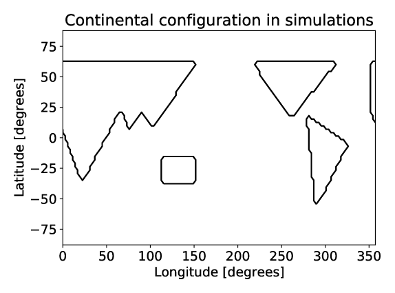
Figure 1: The continental configuration used in the presented simulations.

Radiative transfer calculations coupled to Isca’s dynamics are carried out with the socrates code (Edwards & Slingo, 1996), using the correlated-k method to solve the plane-parallel, two-stream approximated radiative transfer equation with scattering for atmospheres irradiated by a solar (G-star) spectrum. In high-instellation, low-$p$CO₂ simulations, we used the standard, validated spectral files used by the UK Met Office in the latest iteration of its Unified Model to simulate Earth’s climate (Walters et al., 2019). For high $p$CO₂ model configurations, we used a spectral file from NASA GISS’s ROCKE-3D (Way et al., 2017) database and created for GCM modeling of the ancient Martian atmosphere, similar (though not identical) in construction to that used in Guzewich et al. (2021) (Eric T. Wolf, personal communication). The file is valid for atmospheres up to 10 bars with $>90\%$ CO₂ and temperatures up to 400 K, with some loss of accuracy above 310 K (though we compared TOA fluxes from this model at high temperatures with those generated using a high resolution 318 band spectral file used in Graham et al. (2022) and found the output from the GCM stayed within 5 W m^-2 of the higher resolution calculations). Rayleigh scattering is interactively calculated with coefficients included in socrates for the relevant gases. For CO₂, opacity coefficients were tabulated and derived from the HITRAN database, making use of line-by-line and collision-induced absorption coefficients, along with sub-Lorentzian line-broadening and self-broadening (Perrin & Hartmann, 1989; Baranov et al., 2004; Gordon et al., 2017), and similarly for H₂O, which included line-by-line and collision-induced absorption coefficients and the H₂O MT-CKD continuum, along with broadening coefficients that are unfortunately calculated with respect to Earth air (Mlawer et al., 2012; Gordon et al., 2017), which may somewhat underestimate water opacities at hig h temperatures (Pierrehumbert, 2010). We note that the CO₂ continuum spectrum is uncertain at high temperatures and pressures, which introduces a potentially significant source of error into our calculations (e.g. Halevy et al., 2009; Wordsworth et al., 2010).

	$\mathbf{\mathit{S}}$ [W m-2]:
	675	750	800	1000	1250
$\mathbf{\mathit{p}}$CO2 [bars]:
2$\times 10^{-4}$					✓
3$\times 10^{-4}$					✓
4$\times 10^{-4}$					✓
1		✓	✓	✓
2	✓	✓	✓	✓
3	✓	✓	✓
4	✓

Table 1: Table with checkmarks indicating the combinations of substellar TOA instellation ($S$; columns) and CO₂ partial pressure ($p$CO₂; rows) used in the simulations presented in this study. The simulations with $p$CO${}_{2}<$ 1 bar (marked green) are supplemented by 1 bar of N₂, while those with $p$CO${}_{2}>$1 bar have no atmospheric N₂.

With one exception, each simulation was run until the TOA and surface energy fluxes were balanced to within $<$1$\%$ and then for at least a year further, with stated results coming from averages over the final year of data for each simulation. The three low $p$CO₂ simulations have N₂-dominated atmospheres, surface pressures of 1 bar, and CO₂ concentrations of 200, 300, and 400 parts per million by volume (ppmv), all irradiated by TOA instellation of $S=1250$ W m^-2. The eleven high $p$CO₂ simulations have TOA substellar shortwave instellations of $S=675$, 750, 800 or 1000 W m^-2 and CO₂ partial pressures of one, two, three, or four bars (see Table 1). All simulations have atmospheric H₂O content determined by Isca’s hydrologic cycle. The simulation with three bars of CO₂ irradiated by $S=800$ W m^-2 is the exception to the statement about equilibration of fluxes to within $<1\%$, as one of its grid cells exceeded the model’ s temperature limit of 350 K during spin-up while TOA fluxes were still 1.9$\%$ out of balance. Thus results from that simulation are averaged over a period during which the planetary surface was still gradually heating, with a 2$\%$ TOA flux imbalance, instead of $<1\%$ like the others. Based on the behavior of the other simulations, the model would have warmed another Kelvin or two in the mean if it had been able to run to equilibrium, a small error unlikely to have any impact on the qualitative trends demonstrated here.

2.2 Weathering models

For both the MAC and the WHAK formulation, we calculate a weathering flux ($F_{\rm sil}$ [moles m^-2 yr^-1]) in any grid cell that 1.) has land, 2.) has a surface temperature above the triple point of water, 273.15 K, and 3.) has a local precipitation flux greater than zero. Here, we focus exclusively on continental silicate weathering, ignoring the potential contribution of analogous reactions on the seafloor (e.g. Coogan & Gillis, 2013) due to lack of clarity about the strength of this feedback, but we return to the issue of seafloor weathering in Section 5. A global weathering rate ($W_{\rm tot}$ [moles yr^-1]) is calculated by multiplying each cell’s weathering flux by the surface area ($dA$) of the grid cell and then adding them all together i.e.

$$W_{\rm tot}=\sum_{\mathrm{lat,lon}}F_{\rm sil}dA$$ (2)

rendering the CO₂ consumption rate for a planet with the assumed weathering properties and background climate.

For silicate weathering to serve as a stabilizing negative feedback on planetary climate, it must act to maintain the climate at a set-point determined by the properties of the silicates being weathered, the orbital and surface properties of the planet, and the planet’s CO₂ outgassing rate. This requires global weathering to accelerate with increases to $p$CO₂ and surface temperature. Under such conditions, if a planet has its climate perturbed in a way that makes its weathering rate fall below its CO₂ outgassing rate, CO₂ will be consumed more slowly than it is added to the atmosphere, leading to net CO₂ growth and surface warming until the global weathering rate has accelerated to the point that it is equal to outgassing, whence the atmospheric CO₂ content will stop evolving. In the opposite scenario, where global weathering decelerates in response to increases in $p$CO₂ and surface temperature, the process becomes a destabilizing feedback. In this case , the carbon/climate equilibrium where weathering matches outgassing is unstable. If $p\mathrm{CO_{2}}$ is displaced to the high side of the equilibrium, weathering becomes less than outgassing, $\mathrm{CO_{2}}$ would accumulate, and temperature would increase until something occurs to arrest the process (e.g. the planetary interior running out of $\mathrm{CO_{2}}$). If $p\mathrm{CO_{2}}$ is displaced to the low side of the equilibrium, weathering will exceed outgassing and $p\mathrm{CO_{2}}$ will continue to decrease until a stable low $p\mathrm{CO_{2}}$ climate (possibly a Snowball) is reached.

Thus the stability of a carbon cycle at a given instellation can be determined by calculating how the weathering rate changes with $p$CO₂ (the so-called “weathering curve” (Penman et al., 2020)): if weathering rate is positively correlated with $p$CO₂, it acts as a stabilizing negative feedback, but if it is inversely correlated with $p$CO₂ it acts as a destabilizing positive feedback. So, rather than carry out very long asynchronously-coupled simulations evolving atmospheric $p$CO₂ according to the balance between an assumed outgassing flux and a calculated weathering flux, we take the much simpler approach of doing a handful of simulations at a variety of $p$CO₂ and diagnosing the global weathering rates from these “snapshots.” Simply determining the sign of the slope of the weathering curve at a given instellation is sufficient for determining the stability of the carbon cycle. Under stabilizing conditions, imposing an outgassing rate would inexorab ly drive the $p$CO₂ to the level that generates a weathering rate equal to the assumed outgassing rate. Under destabilizing conditions, the final outcome would be determined by the initial conditions, i.e. whether the planet started off with outgassing greater than or smaller than its initial weathering rate.

In the next subsections, we describe how the two weathering models we deploy (MAC and WHAK) calculate $F_{\rm sil}$ as a function of local climate.

2.2.1 WHAK

The formulation of weathering developed in Walker et al. (1981) (WHAK) is the basis for the calculations in most previous exoplanet weathering/climate studies, including the few that have employed 3D GCMs (e.g. Edson et al., 2012; Paradise & Menou, 2017; Jansen et al., 2019; Paradise et al., 2019). We carry out calculations using the WHAK weathering formulation to compare with results from the MAC model, which is more closely tied to the underlying weathering chemistry than WHAK. WHAK weathering implicitly assumes silicate weathering rates are limited by the kinetics of silicate dissolution, which produces an exponential dependence on temperature. WHAK also includes a power-law dependence on CO₂ partial pressure ($p$CO₂). We represent this as:

$$F_{\mathrm{sil}}=\frac{W_{\rm ref}}{\gamma_{\rm Earth}\times 4\pi R_{\rm Earth}^{2}}\exp{(\frac{T-T_{\rm ref}}{T_{\mathrm{e}}})}(\frac{\text{pCO}_{2}}{\text{pCO}_{2,\rm ref}})^{\beta}$$ (3)

where $F_{\mathrm{sil}}$ [mol m^-2 yr ^-1] is the weathering flux from a grid cell, i.e. the number of divalent cations (which react with oceanic carbon to form carbonate minerals, ultimately removing CO₂ from the atmosphere) delivered to the ocean per unit time per unit land area in a given grid cell; $W_{\rm ref}$ is a reference global weathering rate (assumed equal to an estimate of Earth’s modern-day CO₂ outgassing, see Table LABEL:tab:ch4_weathering_values); $\gamma_{\rm Earth}\times 4\pi R_{\rm Earth}^{2}$ is the approximate land area of the Earth, calculated by multiplying its land fraction ($\gamma_{\rm Earth}$) by its surface area ($4\pi R_{\rm Earth}^{2}$), necessary for translating $W_{\rm ref}$ from a global weathering rate into a weathering flux per unit land area; $T$ [K] is the local surface temperature in a grid box; $T_{\mathrm{e}}$ is the e-folding temperature for the weathering reaction; $p$CO₂ [bar] is the CO₂ partial pressure; and $\beta$ is th e power-law dependence on $p$CO₂. The values of $T_{e}$ and $\beta$, which determine the sensitivity of the reaction rate to changes in temperature and $p$CO₂, vary considerably for different silicate minerals. We choose the default values listed in Table LABEL:tab:ch4_weathering_values based on results from laboratory silicate dissolution experiments (e.g. Schott & Berner, 1985; Brady, 1991; Knauss et al., 1993; Oxburgh et al., 1994; Welch & Ullman, 1996; Chen & Brantley, 1998; Weissbart & Rimstidt, 2000; Oelkers & Schott, 2001; Palandri & Kharaka, 2004; Carroll & Knauss, 2005; Golubev et al., 2005; Bandstra & Brantley, 2008; Brantley et al., 2008). In this formulation of WHAK, we ignore the runoff-dependence assumed in the original formulation (Walker et al., 1981), as it has been demonstrated not to substantially impact global weathering rates, which are dominated by the exponential temperature dependence and power-law CO₂ dependence (Abbot et al., 2012). Further, truly kinetically-limited weathering would not be impacted by changes to runoff, since the weathering rate would instead be determined by the rate of production of cations through silicate dissolution. Absent an accompanying change to temperature or $p$CO₂, any change to runoff above zero would simply change the dilution of weathering products without ultimately altering their rate of production or delivery to the ocean.

2.2.2 MAC

The other weathering model we apply in our simulations is modified from (Graham & Pierrehumbert, 2020), which applied a global-mean version of the MAC weathering model (Maher & Chamberlain, 2014; Winnick & Maher, 2018) to calculate global weathering fluxes from models of Earth-like exoplanets. The MAC model accounts for the impact of clay formation in the weathering zone, which sets a maximum concentration on weathering products in runoff, drastically increasing the importance of hydrology for determining weathering fluxes when water moves through the weathering zone at a rate that allows for weathering products to reach the maximum chemically-equilibrated concentration. In this paper, rather than a global-mean formulation, we apply the weathering model from Graham & Pierrehumbert (2020) locally in each land grid cell, with the weathering flux in a given cell determined by the parameterized silicate properties, local H₂O precipitation flux, surface temperature, and $p$CO₂:

$$F_{\rm sil} =\frac{\alpha}{[k_{\rm eff}]^{-1}+mAt_{\rm s}+\alpha[qC_{\rm eq}]^{-1}},$$ (4)

where $F_{\rm sil}$ [mol m^-2 yr^-1] is the weathering flux from a given cell as above; $\alpha$ is a parameter that captures the effects of various weathering zone properties like characteristic water flow length scale, porosity, ratio of mineral mass to fluid volume, and the mass fraction of minerals in the weathering zone that are weatherable (see Graham & Pierrehumbert (2020) for a full explanation); $k_{\rm eff}=k_{\rm eff,ref}\exp{\left(\frac{T_{\rm surf}-T_{\rm surf,ref}}{T_{e}}\right)}\left(\frac{p\text{CO}_{2}}{p\text{CO}_{\rm 2,ref}}\right)^{\beta}$ [mol m^-2 yr^-1] is the effective kinetic weathering rate, i.e. the weathering rate in the absence of chemical equilibration with clay formation (Walker et al., 1981); $m$ [kg mol^-1] is the average molar mass of minerals being weathered; $A$ [m² kg^-1] is the average specific surface area of the minerals being weathered; $t_{s}$ [yr] is the mean age of the material being weath ered; $q$ [m yr^-1] is the flux of water through the grid cell, given by the precipitation in that grid cell output by the GCM; and $C_{\rm eq}=\Lambda(\text{{p}CO}_{2})^{n}$ [mol m^-3] is the maximum concentration of divalent cations in the water passing through weathering zones, as determined by chemical equilibrium between dissolving silicates and the secondary minerals (clays) that form from their products. The default values of all constants are given in Table LABEL:tab:ch4_weathering_values.

By equating local precipitation and $q$, we are assuming that any rain that falls on land drives weathering that delivers solutes to the ocean, i.e. that all precipitation is converted to runoff. Thus these calculations provide an upper limit on weathering fluxes and the efficiency of MAC weathering as a climate feedback with a given set of parameters, as smaller rates of runoff to the ocean would reduce weathering rates. On modern Earth, 20-26$\%$ of precipitation falling on land may be converted to runoff (Ghiggi et al., 2019; Graham & Pierrehumbert, 2020; Coy, 2022), but this value is likely to be heavily dependent on factors like topography, surface temperature, and background atmosphere. As long as runoff is largely monotonic with precipitation, as seems likely (Le Hir et al., 2009; Ghiggi et al., 2019) (though it is unclear whether this must be the case (O’Gorman et al., 2012)), the qualitative behavior we describe should hold. Smaller rates of conversion from rain to run off exacerbate the severity of the mechanism explored here by allowing the energetically-limited regime to be accessed under smaller background CO₂ outgassing rates.

3 Results

3.1 Surface temperature

The mean climate states and CO₂ equilibrium climate sensitivities (ECS) of the simulations are in line with previously published estimates.

The ECS is the steady-state change in global-mean surface temperature from a doubling of atmospheric CO₂, commonly used in studies of Earth’s climate (Knutti et al., 2017; Romps, 2020; Goodwin, 2021). The modern Earth’s ECS is generally estimated to fall between 1.5 K and 4.5 K per doubling (e.g. Knutti et al., 2017). This is consistent with the global-mean temperature behavior of our low-$p$CO₂ simulations, which warmed from 298.1 to 301.5 K as CO₂ was doubled from 200 ppmv to 400 ppmv (see green line and dots in Fig. 2), indicating a reasonable ECS of 3.4 K. These simulations are substantially hotter than the modern Earth despite receiving 8$\%$ less TOA instellation because they lack clouds and the surface has a uniform, dark albedo of 0.05, resulting in planetary albedo of 0.1 due to N₂’s modest Rayleigh scattering effect, in contrast to Earth’s cloud- and ice-maintained albedo of 0.29 (Stephens et al., 2015). None of the low-$p$CO₂ simulations displays temperatures below freezing on any landmass, and in each case the fraction of planetary surface area below freezing at the poles is small (4.2$\%$, 2.5$\%$, and 1.7$\%$ for the 200 ppmv, 300 ppmv, and 400 ppmv simulations respectively).

In climate simulations with very high CO₂, ECS is known to increase as a function of $p$CO₂ due to the increasing importance of self-broadening and activation of spectral regions that are minor at lower pressures (e.g. Halevy et al., 2009; Pierrehumbert, 2010; Russell et al., 2013; Wordsworth & Pierrehumbert, 2013; Ramirez et al., 2014; Wolf et al., 2018; Graham, 2021). Our high $p$CO₂ simulations reflect this behavior, with all displaying an ECS of $\approx$15 K (see blue, cyan, magenta, and red lines with dots in Fig. 2). This is consistent with the behavior of GCM simulations of early Earth atmospheres with instellations slightly larger and $p$CO₂ levels slightly lower than those presented here (Wolf et al., 2018), as well as with ECS values calculated using a polynomial fit (Kadoya & Tajika, 2019) to radiative-convective column model output (Kopparapu et al., 2013) with 1 bar N₂, saturated H₂O, and up to 10 bars CO₂ (Graham, 2021). None of the pr esented high-$p$CO₂ simulations has temperatures below freezing on any landmass, and only the 1 bar, $S=750$ W m^-2 has any planetary surface area below freezing (5.2$\%$, at the poles). Finally, as expected, with a given $p$CO₂, increased instellation leads to higher surface temperatures.

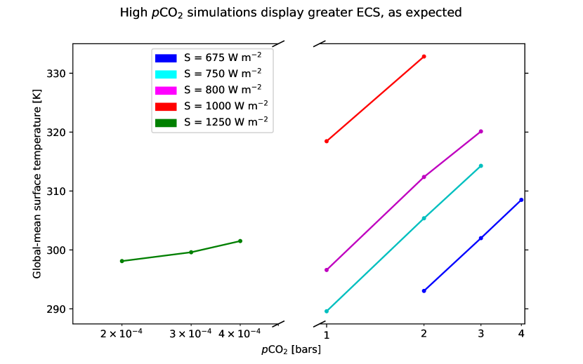
Figure 2: Global-mean surface temperature as a function of $p$CO₂ at various instellations $S$. The low-$p$CO₂, high-instellation simulations display an ECS of 3.4 K, close to estimates of the modern Earth’s (1.5 to 4.5 K). The high-$p$CO₂, low-instellation simulations all display ECS values of around 15 K due to CO₂’s self-broadening effect. Blue corresponds to $S=675$ W m^-2, cyan to 750 W m^-2, magenta to 800 W m^-2, red to 1000 W m^-2, and green to 1250 W m^-2.

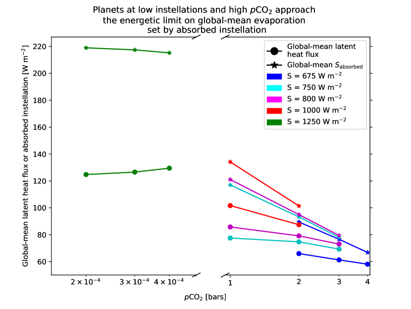
Figure 3: Global-mean absorbed instellation and global-mean upward latent heat flux as functions of $p$CO₂ at various $S$ For low-$p$CO₂, high-instellation simulations, latent heat flux (circle markers) increases with $p$CO₂, but remains far below absorbed instellation (star markers). For high-$p$CO₂, low-instellation simulations, a large majority of their absorbed instellation goes into the latent heat of evaporation. Colors are as in Fig. 2.

3.2 Energy budgets and precipitation

3.2.1 Low $p$CO₂, high instellation

The behavior of the low-$p$CO₂ simulations is largely consistent with expectations from simulations of Earth climate. They approximately reproduce the expected positive trend in global-mean surface latent heat flux (green line with circle markers in Fig. 3), the expected negative trend in global-mean upward longwave from the surface (green line with x markers in Fig. 4), and the expected positive trend in precipitation (green lines in Figs. 5 and 6). Averaged across the three low-$p$CO₂ simulations, global-mean latent heat flux and global-mean precipitation both increased by 1.1 $\%$ K^-1, a bit less than the median value of 1.7$\%$ K^-1 found in Earth climate simulations Held & Soden (2006). Despite increasing somewhat with surface temperature, for all three low-$p$CO₂ simulations the latent heat flux remained far below the limit set by $S_{\rm abs}$ (gre en line with star markers in Fig. 3), which decreased slightly in response to CO₂’s growth because of increased atmospheric absorption of instellation by H₂O as specific humidity rose. The total global-mean net upward longwave flux decreased by 8.7 W m^-2 from the 200 ppmv simulation to the 400 ppmv simulation, a somewhat greater reduction than the 4-5 W m^-2 per CO₂ doubling in Earth GCM simulations (e.g. Gutowski Jr et al., 1991; Boer, 1993), but this is to be expected since our low $p$CO₂ simulations have a warmer background climate than Earth, meaning they should experience larger increases in highly opaque lower-tropospheric water vapor for a given change in temperature than cooler Earth simulations because of the exponential dependence of H₂O partial pressure on temperature. The sensible heat flux of the low-$p$CO₂ simulations changes very little as a function of CO₂, with a reduction of $\approx$1 W m^-2 between the 200 pp mv and 300 ppmv simulations, and an increase of $\approx$1 W m^-2 between the 300 ppmv and 400 ppmv simulations (green line with plus-shaped markers in Fig. 4). This contrasts slightly with simulations of Earth, where the surface’s upward sensible heat flux often decreases by $\approx$1 W m^-2 under a doubling of CO₂ (Gutowski Jr et al., 1991; Boer, 1993; Gómez-Leal et al., 2018), consistent across models with fixed sea surface temperatures, slab oceans (like ours), and fully coupled dynamical oceans (Myhre et al., 2017, 2018). This difference may be due to our neglect of topography, or it may be due to the fact that the climates we simulate are slightly warmer than modern Earth, biasing them toward smaller changes in sensible heat flux with surface temperature (Siler et al., 2019). Nonetheless the changes in sensible heat flux are small in magnitude and the flux itself is already a small enough term in the surface budget that it h as no impact on our qualitative results.

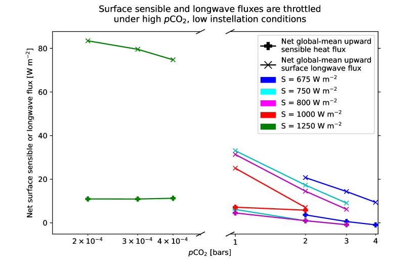
Figure 4: Net upward sensible or longwave heat flux [W m^-2] as a function of $p$CO₂ for simulations at various $S$. For low-$p$CO₂ simulations, the sensible heat flux (x-shaped markers) changes little with $p$CO₂, while for high-$p$CO₂ simulations it drops substantially, even becoming negative in some cases. For both low- and high-$p$CO$-2$ simulations, the longwave flux (plus-shaped markers) decreases with increasing CO₂, as expected. Colors are as in Fig. 2.

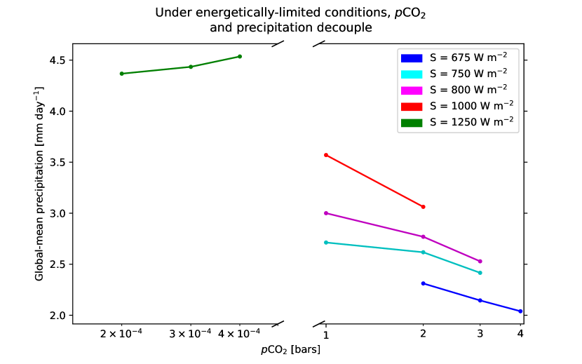
Figure 5: $p$CO₂ vs. global-mean precipitation. For low-$p$CO₂, high-instellation simulations, precipitation increases with $p$CO₂. For high-$p$CO₂, low-instellation simulations in the regime where a large majority of their absorbed instellation goes into driving evaporation, precipitation falls with $p$CO₂. Colors are as in Fig. 2.

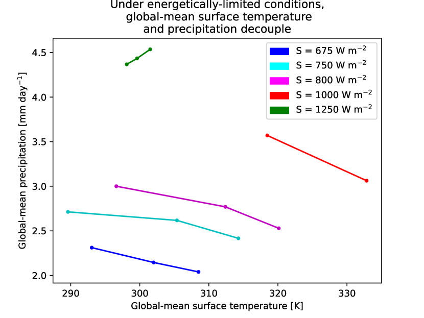
Figure 6: Global-mean surface temperature vs. global-mean precipitation. For low-$p$CO₂, high-instellation simulations, precipitation increases with surface temperature. For high-$p$CO₂, low-instellation simulations in the regime where a large majority of their absorbed instellation goes into driving evaporation, precipitation falls with temperature. Colors are as in Fig. 2.

3.2.2 High $p$CO₂, low instellation

The high $p$CO₂, low-instellation simulations display markedly different behavior from that described above and are clearly operating in a regime where the energetic limit set by absorbed instellation exerts substantial influence. For all sets of high-$p$CO₂ simulations irradiated by a given $S$, global-mean upward latent heat flux at the surface decreases with increasing $p$CO₂, despite the fact that surface temperature increases substantially (see blue, cyan, magenta, and red lines with circles in Fig. 3). These reductions in latent heat flux are accompanied (and driven) by large reductions in absorbed instellation at the surface (see blue, cyan, magenta, and red lines with stars in Fig. 3) due mostly to increases in albedo from CO₂’s Rayleigh scattering, from values of 0.16-0.17 for the $p$CO₂=1 bar cases, to 0.26-0.27 in the $p$CO₂=3 bars simulations, to 0.30 in the $p$CO₂=4 bars case, consistent with prev ious simulations of planets with extremely high $p$CO₂ (Kasting & Ackerman, 1986; Ramirez et al., 2014). As $p$CO₂ is increased in these simulations, even though the absolute latent heat flux goes down, an increasing proportion of the absorbed instellation at the surface goes into evaporation, with values ranging from 66$\%$ to 92$\%$ for the high-$p$CO₂ cases, compared with a range of 57$\%$ to 60$\%$ for the low-$p$CO₂ simulations (see Table 2). Correspondingly, the sensible and longwave heat flux contributions to the surface energy budgets in the high-$p$CO₂ simulations are substantially reduced in both absolute and relative terms (see blue, cyan, magenta, and red plus-shaped markers and x-shaped markers in Fig. 4). Interestingly, the global-mean sensible heat flux becomes negative (directed into the surface) in the $p$CO₂=3 bars simulations irradiated by $S=750$ W m^-2 and 800 W m^-2 and in the $p$CO₂ =4 bars, $S=675$ W m^-2 simulation, but in each case the net sensible heating of the surface is less than 1 W m^-2.

As implied by the trends in latent heat flux vs $p$CO₂ displayed in Fig. 3, global-mean precipitation rates in the high-$p$CO₂ simulations fall with increasing CO₂ (see blue, cyan, magenta, and red lines in Fig. 5). This results in counterintuitive behavior, driving precipitation rates that decrease with increasing surface temperature (see blue, cyan, magenta, and red lines in Fig. 6). Despite some high-$p$CO₂ simulations having surface temperatures much larger than the low-$p$CO₂ simulations, the low-$p$CO₂ simulations all have global-mean precipitation rates larger than any of the high-$p$CO₂ simulations, consistent with the fact that the low-$p$CO₂ precipitation rates are sustained by latent heat fluxes larger than the $S_{\rm abs}$ received by any of the high-$p$CO₂ simulations except the $p$CO₂=1 bar, $S=1000$ W m^-2 case (compare green line with circles to blue, cy an, magenta, and red lines with stars in Fig. 3). In the next section we explore the implications of this energetically-limited precipitation behavior for the functioning of the carbon cycle.

	$\mathbf{\mathit{S}}$ [W m-2]:
	675	750	800	1000	1250
$\mathbf{\mathit{p}}$CO2 [bars]:
2$\times 10^{-4}$					0.57
3$\times 10^{-4}$					0.58
4$\times 10^{-4}$					0.60
1		0.66	0.71	0.76
2	0.74	0.80	0.83	0.86
3	0.80	0.89	0.92
4	0.87

Table 2: Fraction of absorbed instellation going into evaporation ($\frac{L}{S_{\rm abs}}$). Table layout identical to Table 1 except $\frac{L}{S_{\rm abs}}$ values replace checkmarks.

3.3 Weathering rates

In this Section we will present estimates of weathering rates based on output fields from the GCM simulations described above, with weathering fluxes calculated according to both the WHAK and MAC formulations. Sensitivity tests varying the parameters in the weathering models within plausible ranges generated fairly large changes in absolute fluxes but did not affect the qualitative picture presented here.

3.3.1 WHAK weathering

When weathering is calculated according to the WHAK formulation (equation 3), the weathering rate increases strongly in response to increases in $p$CO₂ and $S$ for all simulations, regardless of initial $p$CO₂ or instellation (see Fig. 7). This makes sense, given the WHAK formulation’s exponential temperature-dependence and power-law $p$CO₂ dependence, both of which naturally produce big increases in weathering fluxes for modest changes in temperature and/or $p$CO₂. The increases produced by this model are unrealistically large even if we take the WHAK formulation at face value, as the global rate of rock uplift sets a “supply limit” on the rate of silicate weathering of $\mathcal{O}$(100) trillion moles of CO₂ per year on Earth [Tmol yr^-1] (e.g. Kump, 2018), but the positive slope of the curves in Fig. 7 confirms in principle the continued operation of WHAK weathering as a negative feedb ack even under high-$p$CO₂, low-instellation conditions where energetically-limited precipitation is relevant. Earth’s outgassing rate is generally estimated to lie somewhere between 3 and 15 Tmol yr^-1 (Coogan & Gillis, 2020), substantially smaller than even the smallest weathering rate produced by the these simulations, but this is due to our mostly arbitrary choice of weathering constant $W_{\rm ref}$ in equation 3. A smaller $W_{\rm ref}$ would produce proportionally smaller weathering rates without changing the qualitative trends in weathering vs. $p$CO₂.

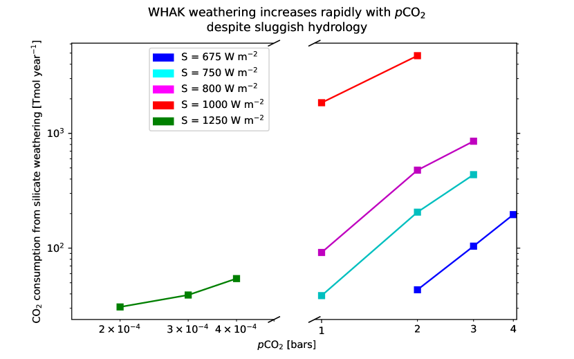
Figure 7: Global WHAK weathering rates [Tmol yr^-1] vs. $p$CO₂ for a variety of instellations. Weathering fluxes are calculated according to the WHAK formulation (equation 3). For all simulations, the weathering rate increases with CO₂. Colors are as in Fig. 2.

3.3.2 MAC weathering

With MAC weathering, the low $p$CO₂ simulations respond essentially as expected (Fig. 8). Although the strength of the weathering response to the changes in the surface climate is much weaker than in the WHAK case, the weathering rate in the low $p$CO₂ simulations still increases with increasing $p$CO₂, producing a stabilizing negative feedback. This provides tentative evidence that MAC-style continental weathering may be able to stabilize the climates of planets under Earth-like conditions of high instellation and low $p$CO₂.

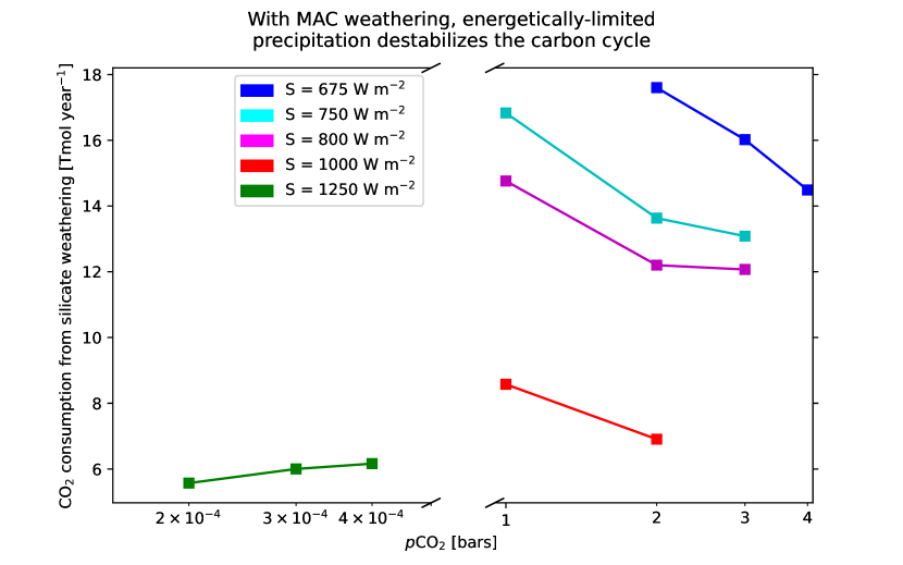
Figure 8: Global MAC weathering rates with fiducial parameter values [Tmol yr^-1] vs. $p$CO₂ for a variety of instellations. Weathering fluxes are calculated according to the MAC formulation (equation 4). For low-$p$CO₂ simulations, the weathering rate increases with CO₂, while for high-$p$CO₂ simulations weathering decreases with increasing CO₂. Colors are as in Fig. 2.

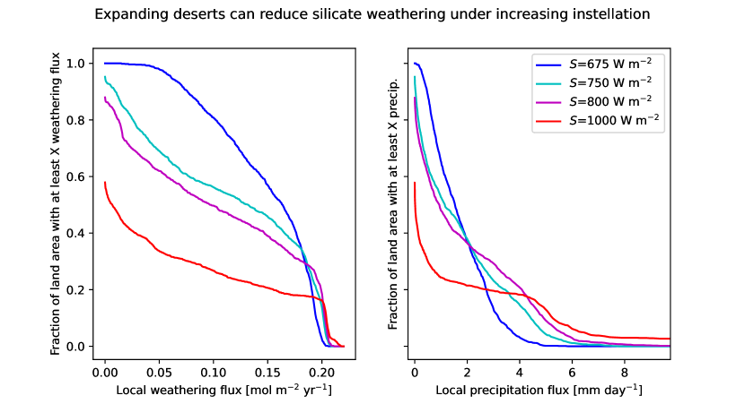
Figure 9: The change in spatial distribution of MAC weathering (left) and precipitation (right) that accompanies increasing TOA instellation Results shown are for simulations with $p$CO₂ = 2 bars and $S=675$ W m^-2 (blue), $S=750$ W m^-2 (cyan), $S=800$ W m^-2 (magenta), and $S=1000$ W m^-2 (red). The y-value of a curve represents the fraction of land with at least as much weathering flux (left) or precipitation (right) as the corresponding x-axis value. Even though the total global precipitation increases as $S$ increases, the total global weathering rate decreases because less land is receiving substantial precipitation. See Section 3.3. Colors are as in Fig. 2.

In contrast, the high $p$CO₂, low instellation simulations in the energetically-limited regime produce a drastically different carbon cycle than the WHAK calculations or the low-$p$CO₂ MAC calculations would suggest. While they do display somewhat higher weathering rates than the low $p$CO₂ simulations due to the thermodynamic $p$CO₂-dependence of the maximum concentration of weathering products in runoff ($C_{\rm eq}$ in equation 4, a much weaker effect than that of the $p$CO₂-dependence of WHAK weathering represented by $\beta$ in equation 3), all of the high-$p$CO₂ simulations display the opposite response to further increases in CO₂: at a given $S$, as $p$CO₂ increases (along with surface temperature), the global weathering rate goes down (see blue, cyan, magenta, and red lines in Fig. 8). As described in Section 2.2, anti-correlation between global weathering rates and $p$CO₂ destabilizes the carbon cycle, so the high-$p$CO₂ simulations are all displaying a defective climate thermostat with a positive feedback that would likely induce runaway climate heating or cooling. Although this result runs counter to Earth-based intuitions, the unusual trends in $p$CO₂ vs. weathering make sense given the increased importance of hydrologic cycling in the MAC weathering framework and the reduction in global-mean precipitation triggered by reduced $S_{\rm abs}$.

Another unexpected weathering trend appears in the set of high $p$CO₂ simulations: holding CO₂ constant, the global weathering rate goes down even as instellation rises and drives both surface temperature (Fig. 2) and global-mean precipitation (Fig. 5) upward with it. This trend obviously cannot be explained by a global-mean argument, since all of the variables that directly control weathering are, in bulk, either increasing (i.e. $q$ and surface temperature) or staying the same (i.e. $p$CO₂) as $S$ is increased. Instead, the explanation lies in the intensification of moisture extremes expected in warming climates from simple thermodynamic considerations (Held & Soden, 2006; Allan et al., 2020), often referred to by the phrase “wet gets wetter, dry gets drier” (WGWDGD) in discussions of Earth climate (Allan et al., 2020) though over the past several years it has become clear that this basic picture does not hold as wel l over land in Earth simulations as it does over the ocean (Byrne & O’Gorman, 2015; Feng & Zhang, 2015; Allan et al., 2020). Although WGWDGD does not perfectly describe the moisture response over land in Earth simulations under the (comparatively) small climate perturbations projected for this century, it quite accurately describes the behavior of the precipitation in our high-$p$CO₂ simulations as $S$ is increased.

In other words, although the total global precipitation flux increases with $S$ in our high-$p$CO₂ simulations, it also becomes concentrated onto a smaller area, meaning deserts expand as $S$ goes up. For example, in the $S=675$ W m^-2, $p$CO₂=2 bars case, over half of the planet’s land area receives more than 1 mm day^-1 precipitation, whereas only about a quarter of the land area in $S=1000$ W m^-2 receives that much water (see right side of Fig. 9). This is compensated by an increasing fraction of landmass with high precipitation fluxes, i.e. only $\approx$5$\%$ of the landmass in the aforementioned $S=675$ W m^-2 simulation exceeds 4 mm day^-1 of rain, but about 20$\%$ of the landmass in the $1000$ W m^-2 simulation meets that criterion, and higher $S$ generally leads to a longer “tail” of landmass with large local precipitation fluxes. As can be seen by comparing the weathering flux curves on the left side of Fig. 9 with the precipitation flux curves on the right, local weathering tracks local precipitation quite directly, so it might seem that the long tail of high precipitation over land should more than make up for the expansion in dry areas. However, past a point determined by balance between the kinetics of silicate dissolution and the timescale and surface area of contact between water and dissolving silicates, extremely high precipitation has diminishing returns in terms of weathering rates (Maher & Chamberlain, 2014). If water flushes out a weathering zone rapidly enough, the system becomes kinetically limited and any further increases to the water’s flow rate will simply change the degree of dilution of weathering products rather than increasing their flux. We can see this effect in Fig. 9 where all of the local weathering fluxes drop off abruptly around 0.2 mol m^-2 yr even though a direct scaling of weathering flux with water flux would suggest a long tail of much larger local fluxes for the $S=1000$ W m^-2 simulation. Interestingly, although the precipitation rate and $S_{\rm abs}$ both increase as $S$ goes up, simulations at a given $p$CO₂ still move progressively closer to the energetic limit set by $S_{\rm abs}$ (see Table 2), which may play a role in constraining the areal extent of precipitation over land and forcing the growth of desert regions. The potential for reduction in weathering with increased $S$ is another destabilizing influence in the carbon cycle, since even with a functional negative feedback at a given instellation (i.e. positive slope in weathering vs. $p$CO₂), this effect would force $p$CO₂ to higher equilibria at higher instellations, likely significantly reducing a planet’s habitable lifetime under increasing host star luminosity.

4 Discussion

4.1 Catastrophic carbon cycle hysteresis

With MAC-style, hydrologically-regulated weathering, energetically-limited precipitation can cause a breakdown of the negative feedback on climate that emerges within the carbonate-silicate cycle. Our high-$p$CO₂, low-instellation simulations displayed reductions in weathering with CO₂ growth, opposite the trend required to stabilize climate by balancing CO₂ sequestration against CO₂ outgassing. This implies that in the portion of the instellation-$\mathrm{CO_{2}}$ space we have probed, which are generally characteristic of the outer reaches of the conventional HZ, coupled climate/carbon-cycle equilibria are unstable. The instability is not just a local instability to infinitesimal displacements. The unstable equilibria represent the attractor basin boundary between low $\mathrm{CO_{2}}$ states when the system is displaced on the cold side, and states with very high $\mathrm{CO_{2}}$ when the system is displaced on the warm side. The unstable branch extends over the e ntire range of $\mathrm{CO_{2}}$ for which weathering decreases with $\mathrm{CO_{2}}$. For each instellation considered, weathering decreases with increasing $\mathrm{CO_{2}}$ in the high $\mathrm{CO_{2}}$ regime. However, in the colder low $\mathrm{CO_{2}}$ regime, weathering is expected to increase with $\mathrm{CO_{2}}$ because precipitation is not subject to an energy limit. (We have demonstrated that explicitly only for one instellation value). Based on these two end-member behaviors, it is inferred that there is a maximum weathering rate which, for the lower ranges of instellation we have considered, occurs at a $p\mathrm{CO_{2}}$ somewhere below 1 bar.

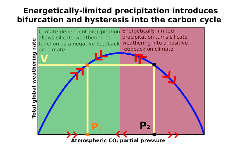
Figure 10: A schematic of the saddle node bifurcation in the carbon cycle suggested by our simulations. The blue curve represents the global weathering rate as a function of $p$CO₂. Weathering increases with increasing $p$CO₂ (and surface temperature) in the green zone, and it decreases with increasing $p$CO₂ (and surface temperature) in the red zone. Weathering rates are equal to outgassing ($V$) at $p$CO₂=$P_{1}$ (orange) and at $p$CO₂=$P_{2}$ (black). The $P_{1}$ equilibrium is stable because weathering acts as a negative feedback in that regime, while the $P_{2}$ equilibrium is unstable due to silicate weathering’s positive feedback behavior. The red arrows indicate the directions CO₂ and weathering would evolve for a climate intialized from various points relative to the two equilibria.

The inferred structure of the weathering curve governing climate/carbon equilibrium is shown schematically in Fig. 10, assuming there to be only one local maximum of weathering. The value of $p\mathrm{CO_{2}}$ at which peak weathering occurs, and the height of the peak, depend on instellation. Our simulations have probed just a portion of the relevant instellation space, and only a portion of the right-hand half of the curve where weathering decreases with $p\mathrm{CO_{2}}$. In particular, we have not located the peak of the weathering curve, which occurs in the gap between our low and high $p\mathrm{CO_{2}}$ simulations. The geometry of the weathering curve indicates the presence of a saddle-node bifurcation (e.g. Strogatz, 1994) in the climate/carbon equilibrium. For a given volcanic outgassing rate below peak weathering (indicated by the horizontal line labeled ”V” in the figure), there are two equilibria. The equilibrium $P_{2}$ to the right is unstable; this is the unstable high $p\mathrm{CO_{2}}$ equilibrium we have identified in our simulations. If the system initially has $p\mathrm{CO_{2}}$ anywhere to the left of $P_{2}$, it will be attracted to the stable low $p\mathrm{CO_{2}}$ equilibrium $P_{1}$ Because our simulations have not located the peak, we cannot determine whether the stable state $P_{1}$ is a Snowball or a habitable low $p\mathrm{CO_{2}}$ state with above-freezing conditions.

If the system starts somewhat to the right of $P_{2}$, then $\mathrm{CO_{2}}$ will accumulate until something arrests the process at higher $p\mathrm{CO_{2}}$. This could terminate at complete degassing of the interior $\mathrm{CO_{2}}$ reservoir, leading to a hot Venus-like state with a thick gaseous atmosphere, or a more temperate state where $\mathrm{CO_{2}}$ accumulates in the form of a liquid ocean, depending on instellation as in Graham et al. (2022). Alternately, it is possible that the weathering curve turns around at sufficiently high $p\mathrm{CO_{2}}$, allowing a new stabke high $p\mathrm{CO_{2}}$ equilibrium to exist, though possibly at an uninhabitably hot temperature. Because the processes leading to the decrease of weathering with $p\mathrm{CO_{2}}$ persist and even accentuate at higher values than we have probed, we think this unlikely, but it is a possibility that cannot be ruled out at present. In any event, the unstable equilibrium $P_{2}$ is a basin boundary between stab le low and high $p\mathrm{CO_{2}}$ states.

It is generic to the geometry of saddle-node bifurcations that the system supports hysteresis. Suppose the planet starts in the stable equilibrium $P_{1}$ at a time when volcanic outgassing is relatively weak. If outgassing increases subsequently, and exceeds the peak of the weathering curve, then the system will transition to a stable high $p\mathrm{CO_{2}}$ equilibrium somewhere past the right edge of the diagram. Because any state to the right of $P_{2}$ will be attracted to the high $p\mathrm{CO_{2}}$ state, volcanic outgassing would need to be reduced to below its original value in order to restore a stable low $p\mathrm{CO_{2}}$ state. Because the peak of the weathering curve depends on instellation, it is also possible for such hysteresis loops to occur for fixed outgassing, as a result of evolution of stellar luminosity. Our simulations indicate that increasing instellation in the high $p\mathrm{CO_{2}}$ states decreases weathering, and so likely reduces the peak weathering. Thi s scenario could lead to a new form of habitability termination as a G or F star increases in luminosity over its main sequence lifetime.

There are additional pathways into the energetically-limited regime that do not require any changes to outgassing or instellation. For example, if the $p$CO₂ necessary to deglaciate a planet in a snowball state lies at $p$CO${}_{2}>P_{2}$ (black markers in Fig. 10), then escape from global glaciation due to reduced weathering in icy conditions could counter-intuitively propel a previously temperate planet into a death spiral of uncontrolled heating. Upon accumulating enough CO₂ to deglaciate, rather than weathering away the excess to return to a temperate climate, runaway CO₂ accumulation would ensue due to the processes described above for planets initialized from $p$CO${}_{2}>P_{2}$. Similarly, if Earth-like planets outgas massive CO₂ atmospheres during their magma ocean phases like some models suggest (e.g. Solomatova & Caracas, 2021), some may become “locked in” to this early, hot, high-$p$CO₂ phase, since their weathering rates after magma ocean crystallization and water ocean condensation might remain pinned below their early outgassing rates due to energetically-constrained precipitation. However, expectations that planets will also face a large flux of impacts producing highly weatherable ejecta in the early stages after planet formation (e.g. Kadoya et al., 2020) may help mitigate this danger. Further, at low instellations, deglaciation can be prevented by CO₂ condensation onto the icy planetary surface (Turbet et al., 2017; Kadoya & Tajika, 2019), which may restrict the parameter space that allows for a post-Snowball death spiral.

A more quantitative example of how CO₂ runaway might play out can be illustrated with direct reference to Fig. 8. The $p$CO₂=1 bar, $S=1000$ W m^-2 simulation (red squares in Fig. 8) displays a weathering rate of 8.6 Tmol yr^-1. If we take this as our initial climate state and impose a volcanic CO₂ degassing rate of 10 Tmol yr ^-1, which is well within the range of estimates for Earth’s outgassing rate (Catling & Kasting, 2017; Coogan & Gillis, 2020), the planet’s $p$CO₂ will begin to grow because the flux into the atmosphere is greater than the flux out. Under Earth-like conditions, this would cause warming, an intensification of the hydrological cycle, and an acceleration in weathering (as we see in the low-$p$CO₂ cases, the green squares in Fig. 8), moving the carbon cycle closer to equilibrium, but in this case the opposite happens, with a progressive reduction in the weathering rate as CO₂ accu mulates. By the time our hypothetical $S=1000$ W m^-2 planet had accumulated another bar of CO₂, its weathering rate would have fallen to only 6.9 Tmol yr^-1 (see red square at $p$CO₂=2 bars in Fig. 8). Thus the planet would have a carbon cycle further out of balance with its 10 Tmol yr^-1 outgassing rate than when it started, with no signs of slowing down. We did not carry the $S=1000$ W m^-2 simulations to higher $p$CO₂ because of the temperature constraints of our modeling framework, but even at $p$CO₂=2 bars the planet is verging on inhospitable conditions, with a global-mean surface temperature in excess of 330 K (red dot at $p$CO₂=2 bars in Fig. 2). Assuming the negative weathering trend holds out to even larger $p$CO₂, or at least that the weathering rate remains below the assumed 10 Tmol yr^-1 outgassing rate, the planet would eventually be forced by the carbonate-silicate cycle into an uninhabitably hot st ate, likely continuing to warm until it degassed all of the available CO₂ from its interior, ending up with a dense, steamy, supercritical CO₂/H₂O atmosphere unless some unknown process was triggered along the way that allowed the weathering rate to accelerate back to parity with the outgassing rate. Simulations of water photolysis and hydrogen escape on CO₂-rich planets orbiting G-stars suggest that the upper-atmospheric cold trap generated by the low instellations and high CO₂ partial pressures under consideration would throttle water loss to insignicant levels, allowing these hot, steam-rich surface conditions to persist over geologic timescales (Wordsworth & Pierrehumbert, 2013).

At somewhat lower instellations than $S=1000$ W m^-2, CO₂ condensation at the surface would become a possibility at high enough $p$CO₂, meaning the energetic limit on precipitation presents a pathway to reach the stable CO₂ ocean states proposed in Graham et al. (2022). The mechanism of carbon cycle destabilization suggested in that study was based on the fact that CO₂ becomes a coolant at extremely high partial pressures, which also leads to a slowdown of weathering with $p$CO₂ accumulation but requires much higher CO₂ to initiate than the mechanism discussed here. This means that energetically-limited weathering may increase the probability that low-instellation planets within the HZ end up with CO₂ oceans, with uncertain implications for their habitability. Although CO₂ ocean worlds are restricted to relatively clement climates below 304 K (the critical temperature of CO₂), they would still sport extreme surface pressures (up to 72 bars), an d in the process of accumulating that much CO₂ surface temperatures can peak at extreme levels ($>400$ K) before Rayleigh scattering begins to outweigh CO₂’s greenhouse effect and further accumulation begins to cool the planet (Graham et al., 2022). Intriguingly, some work has suggested that liquid and supercritical CO₂ may be conducive to prebiotic chemistry (Shibuya & Takai, 2022), and supercritical CO₂ may drive rapid carbonate formation (see Section 5 and McGrail et al., 2017), suggesting these worlds may not be as hostile to life as they appear at first.

s debate remains over proxy interpretation (Galili et al., 2019; Vérard & Veizer, 2019; Herwartz et al., 2021), some paleotemperature constraints suggest that the Archean Earth may have had surface temperatures in the vicinity of 340 K (e.g. Lowe et al., 2020; McGunnigle et al., 2022), again presenting the possibility that early Earth may at times have verged on the energetically-limited weathering behavior simulated here. Finally, we note that early Mars, which was irradiated by a lower instellation than any of the planets we modeled, is generally postulated to have had a CO₂-dominated atmosphere, and displays abundant evidence of active hydrologic cycling (e.g. Kite, 2019; Kite et al., 2019, 2021), may be another environment in which energetically-limited precipitation and weathering became relevant.

4.2 Limit cycling?

First, we note that our WHAK weathering results (Fig. 7) are qualitatively consistent with previous WHAK-based exoplanet weathering calculations driven by zero-dimensional (Menou, 2015; Abbot, 2016), one-dimensional (Haqq-Misra et al., 2016; Kadoya & Tajika, 2019), and three-dimensional (Paradise & Menou, 2017) climate models. In all of these cases, the direct power-law dependence of weathering fluxes on $p$CO₂ (the $\beta$ term in eqn. 3) means that planets at lower instellations (where larger $p$CO₂ is necessary to maintain a given surface temperature) display much higher weathering rates under temperate conditions, necessitating colder surface climates to reduce weathering enough to equilibrate with an Earth-like outgassing rate. Under fairly broad combinations of instellation and weathering properties (e.g. Abbot, 2016), this direct $p$CO₂-dependence was suggested to draw CO₂ down to levels that would glaciate pla nets. This led to the prediction that terrestrial planets in the outer reaches of the HZ would spend most of their time in snowball states, punctuated by intermittent periods of temperate surface conditions when cold- and ice-induced slowdowns in weathering allowed CO₂ to build up to high enough levels to achieve deglaciation briefly, at which point weathering would accelerate again and re-glaciate the planet, a periodic process termed “limit cycling” (Menou, 2015; Haqq-Misra et al., 2016). The huge increases in WHAK weathering rates for our high-$p$CO₂ simulations (Fig. 7) are consistent with this picture, though we did not carry out simulations at low enough $p$CO₂ values and surface temperatures to determine whether the WHAK weathering rates would remain extremely high even as the planets approached glaciation.

Compared to the results discussed above, our MAC weathering calculations (see Fig. 8) suggest completely different behavior for planets with CO₂ dominated atmospheres at reduced instellations within the HZ. Although they do display somewhat higher weathering rates than their low-$p$CO₂ counterparts because of the $p$CO₂-dependence of the equilibrium concentration of solutes ($C_{\rm eq}$ in equation 4), the high-$p$CO₂ MAC simulations do not display the orders-of-magnitude increase in weathering compared to cases with lower CO₂ that is seen with WHAK. From this it seems that MAC weathering imparts much less susceptibility to the limit cycling mechanism, which at first glance appears to be a point in favor of climate stability at low instellation. However, the carbon cycle instability discussed in Section 4.1, which sets in under low instellation and high $\mathrm{CO_{2}}$ conditions when using MAC weat hering, has the potential to pose an equal or greater threat to habitability in the outer portions of the conventional HZ. Unlike climate limit cycling, this instability does not depend on glaciation, though the cold-side attractor could in some cases be a Snowball state. In such cases, the $\mathrm{CO_{2}}$ build-up required to trigger deglaciation could be large enough to flip the system into the hot-side high $\mathrm{CO_{2}}$ attractor. Since we have not quantified the hot-side attractor, we have no basis at present to speculate as to whether there are mechanisms that could return the system to a Snowball state and thus lead to a form of climate limit cycling.

The novel carbon cycle instabiity our work has identified suggests mechanisms whereby the geochemical HZ could be significantly contracted relative to the convential HZ which doesn’t take into account geochemical constraints. The extent to which habitability in the outer portions of the conventional HZ is actually threatened is subject, however, to the resolution of a number of caveats.

5 Caveats

In this study, we focused exclusively on modeling continental silicate weathering rates in a significantly simplified cloud-free GCM with a specific, idealized land configuration and an assumption of spatially uniform lithology and soil properties. There are a variety of possibilities that we did not model which could prevent or complicate the carbon cycle destabilization discussed above.

5.1 Mind the gap

The most important limitation in the results presented above is the gap between our low $p\mathrm{CO_{2}}$ simulations and our high $p\mathrm{=}{CO_{2}}$ simulations. This gap was due to technical issues with finding a computationally feasible spectral representation that would enable the radiation code to cover the whole range. Filling in the gap also would require incorporation of ice-albedo feedback, and probably also dynamic ocean effects, in order to resolve the Snowball transition properly.

For our lowest instellation case, 675$\mathrm{W/m^{2}}$, 1D calculations indicate that $p\mathrm{CO_{2}}$ in excess of 1 bar would be necessary to keep the global mean surface temperature above freezing (Fig. 6 Kopparapu, 2013). Our simulations did not probe below 2 bars for this instellation, but at 2 bars the weathering still is strongly increasing as $p\mathrm{CO_{2}}$ decreases, so it is likely that the unstable feedback continues to 1 bar and below. For this case at least, it seems plausible that the low $p\mathrm{CO_{2}}$ attractor is a Snowball. For the higher instellations in our simulations, the actual position of the peak weathering becomes crucial to the question of whether the attractor is a Snowball.

Our suite of simulations also has a gap for $p\mathrm{CO_{2}}$ above 4 bars, so we cannot say where the $p\mathrm{CO_{2}}$ and temperature ultimately land in circumstances where runaway accumulation occurs.

An additional gap in our story is that we have not probed instellations below 675 $W/m^{2}$, whereas the outer edge of the conventional HZ for G stars is in the vicinity of 475$W/m^{2}$, requiring nearly 10 bars of $\mathrm{CO_{2}}$ for its maintainence. Aside from the instellation being lower than we have probed, the $\mathrm{CO_{2}}$ level is somewhat over twice the maximum value we considered. We can not at present rule out the possibility that the climate/carbon equilibrium stabilizes as the outer HZ edge is approached. This in itself would be an interesting state of affairs, leading to the notion of ”habitable bands” rather than a continuous HZ.

At lower instellations than we have probed, which correspond to conditions nearer to the outer edge of the conventional HZ, $\mathrm{CO_{2}}$ condensation will occur for high $\mathrm{CO_{2}}$ states, first in the upper atmosphere and then approaching the ground as instellation decreases. This condensation has the dual effect on the planetary energy budget of keeping the upper atmosphere warmer than it would have been on the noncondensing adiabat, and through the radiative effects of $\mathrm{CO_{2}}$ ice clouds. $\mathrm{CO_{2}}$ ice clouds aloft have a cooling effect through increasing albedo, and a warming effect through their (infrared scattering) greenhouse effect. Regardless of whether the net effect is warming, cooling or neutral, the cloud albedo further reduces the surface instellation, making the energy limit more stringent than in clear sky conditions and thus further reducing weathering as $\mathrm{CO_{2}}$ increases. This would add to the destabilization of the climate-carbon equilibrium.

5.2 Seafloor weathering

One important consideration is the potential contribution of low-temperature off-axis hydrothermal basalt alteration, frequently referred to as “seafloor weathering,” which has been proposed as an alternative or complementary stabilizing, temperature- and $p$CO₂-sensitive CO₂ sequestration flux analogous to the continental weathering feedback (e.g. Francois & Walker, 1992; Brady & Gislason, 1997; Coogan & Gillis, 2013; Coogan & Dosso, 2015; Krissansen-Totton & Catling, 2017; Krissansen-Totton et al., 2018; Coogan & Gillis, 2018; Hayworth & Foley, 2020). Some work has discounted its ability to act as a stabilizing feedback (Caldeira, 1995; Abbot et al., 2012), but these conclusions have been questioned due to laboratory (Brady & Gislason, 1997) and geochemical (Coogan & Gillis, 2013; Coogan & Dosso, 2015; Coogan & Gillis, 2018) data that indicate an appreciable temperature-dependence of seafloor weathering reactions, potentially allowing the process to accelerate under warmer cli mates and operate as a negative feedback, with important implications for the history of Earth (Krissansen-Totton & Catling, 2017; Krissansen-Totton et al., 2018) and the habitability of exoplanets (Hayworth & Foley, 2020; Chambers, 2020). However, these modeling works generally ignore the throttling effect of clay formation which plays such a fundamental role in the weakening of the continental silicate weathering feedback in the MAC framework. If the waters flowing through seafloor basalts tend to reach their equilibrium concentration of weathering products before the formation of carbonates, then without a feedback between porewater flow rates and global surface temperatures there is limited scope for seafloor weathering to operate as a thermostat. Developing a complete MAC-style model of seafloor weathering that accounts for the major controls on porewater flow rates and the precipitation of relevant clay phases, as suggested in Graham & Pierrehumbert (2020), with first ste ps taken in Hakim et al. (2021), is a necessary next step toward evaluating the importance of seafloor weathering to the carbon cycle of Earth and other exoplanets. This is particularly crucial given the fact that clay formation on the seafloor was likely much more efficient in early Earth’s oceans (and in the oceans of abiotic exoplanets) due to the lack of biosilicifying organisms, which maintain the modern Earth’s ocean in a subsaturated state with respect to silica (Siever, 1992; Kalderon-Asael et al., 2021). Silica is one of the weathering products that drives the formation of many of the clays that consume weathering-derived cations and reduce carbonate precipitation, decreasing the effectiveness of weathering at driving carbon sequestration; thus, although seafloor clay precipitation (“reverse weathering”) has been suggested to exert its own form of negative feedback (e.g. Isson & Planavsky, 2018; Krissansen-Totton & Catling, 2020), it may also prevent traditional seafloor we athering from operating efficiently. The net impact on the carbon cycle of weathering-related processes occurring on the seafloor remains unclear (Krissansen-Totton & Catling, 2020).

5.3 Water clouds

In future work, it will be important to determine whether water clouds could stabilize the MAC weathering feedback. Water clouds affect the hydrology because their albedo further reduces the surface instellation. This is true for both boundary layer clouds and clouds aloft, but clouds aloft in addition exert a warming influence through their greenhouse effect, which can partly compensate or even overwhelm the cooling effect of the albedo. We have cited some reasons to suspect that boundary layer water clouds may be absent in a high $p\mathrm{CO_{2}}$ regime, but if they are still present at, e.g., the 1 bar climate but dissipate as $p\mathrm{CO_{2}}$ increases further, than that would partly offset the energy limit effects on precipitation due to the albedo of $\mathrm{CO_{2}}$. Insofar as MAC weathering is more sensitive to hydrology than to direct temperature effects, dissipation of high clouds could have the same effect on weathering, despite their warming influence. In case s where high clouds exert a dominant warming effect, though, the additional warming could enhance the desertification effect which in our simulations contributes to the destabilizing weathering feedback. Generally speaking, it should be noted that the incremental albedo effect of clouds is muted in climates where albedo is already high due to $\mathrm{CO_{2}}$, and that the greenhouse effect of clouds can be muted if they lie below the radiating level of an optically thick $\mathrm{CO_{2}}$ atmosphere.

5.4 Continental configuration

The amount and spatial arrangement of land can have complex and difficult-to-predict impacts on continental weathering rates via changes to runoff and precipitation (Baum et al., 2022). It may be that certain continental configurations tend to produce positive feedback behavior, while others produce negative feedback behavior. Relatedly, topography heavily influences (and is influenced by) precipitation (Roe, 2005) and erosion (Montgomery & Brandon, 2002) rates, which in turn affect the thickness and age of soils (e.g. Heimsath et al., 2000; Owen et al., 2011), with direct impacts on silicate weathering rates (Ferrier & Kirchner, 2008; Hilley et al., 2010; West, 2012; Maher & Chamberlain, 2014). Surface evolution driven by plate movements (e.g. Coy, 2022) means that all of these factors may constantly co-evolve on an Earth-like planet with plate tectonics. Further, planets in the “stagnant lid” mode (no plate tectonics, e. g. Foley, 2019) may display systematic differences in topograpy (Guimond et al., 2022) and outgassing rates (Guimond et al., 2021), likely introducing further major variation into all of these factors controlling weathering rates and climate evolution. Correlations and feedbacks between the many variables controlling weathering fluxes could significantly change the picture we have presented, and a much broader parameter sweep and investigation of these issues is necessary.

5.5 Ocean heat transport

Modeling climate with a slab (as opposed to dynamical) ocean is a significant simplification, but we consider it unlikely to have a large impact on our qualitative results. Note first that our simulations are carried out without a seasonal cycle, so that the ocean response time is immaterial except insofar as it somewhat dampens surface temperature response to synoptic variability. Additionally, study of Earth’s climate suggests that oceans carry a relatively small proportion of meridional heat transport, with the bulk carried by the atmosphere (Trenberth & Caron, 2001). Moreover, there are robust reasons to expect the atmosphere to compensate for absence of ocean heat transport (Farneti & Vallis, 2013).

Nonetheless, ocean heat transport can increase atmospheric water vapor by spreading atmospheric convection out of a planet’s deep tropics, resulting in global-mean warming (Herweijer et al., 2005). Furthermore, in an icy climate, ocean heat transports can have considerable warming effects because a small amount of heat delivered to and under the sea ice margin is very efficient at melting ice (e.g. Rose, 2015). The latter is not a factor in the climates we explore, since they are all too warm to support much ice, but it is well established that ocean heat transport and sea ice dynamics have a strong influence on the the $\mathrm{CO_{2}}$ concentration at which a planet transitions into a Snowball state (Pierrehumbert et al., 2011), generally requiring lower $\mathrm{CO_{2}}$ for global glaciation than is the case for slab models. Inclusion of dynamical ocean and sea ice effects would be crucial in order to definitively answer whether the low $\mathrm{CO_{2}}$ states the unstable system is attracted to on the cold side of the unstable equilibrium are Snowballs. This is a question we do not attempt to resolve in the present simulations. We also note that some simulations of exoplanetary habitability in the middle- and outer-reaches of the HZ have found ocean heat transport to have a major effect on climate by warming the nightsides of synchronously rotating exoplanets, where they do not receive instellation from their parent stars (Yang et al., 2013, 2014; Hu & Yang, 2014; Yang et al., 2019a). However, since our study is concerned with rapidly rotating exoplanets, this mechanism is less crucial.

5.6 Continental lithology

We have considered only one mineral composition for the weatherable surface, but weathering behavior is sensitive to lithology (Hakim et al., 2021). Additionally, the continental crust would typically exhibit considerable spatial variations in lithology, driven by a multitude of tectonic processes. Such variations can accentuate the effect of continental configuration.

A possible exit route from uncontrolled CO₂ accumulation could arise through the power-law dependence of $C_{\rm eq}$ in equation 4 (characterized by exponent $n$ in Table LABEL:tab:ch4_weathering_values), which allows for larger concentrations of weathering products in a given amount of water for planets with larger $p$CO₂, suggesting that further accumulation of CO₂ in the energetically-limited regime could eventually reverse the sign of the weathering curve back into negative feedback territory. This is the mechanism that allowed the subset of simulations that entered the parameterized energetically-limited precipitation regime in the global-mean study of Graham & Pierrehumbert (2020) to avoid runaway CO₂ accumulation, instead equilibrating at hot temperatures with high $p$CO₂. In this scenario, the slope of the blue weathering curve in Fig. 10 would eventually reverse and begin to increase again at high $p$CO₂, introducing a new, stable carbon cycle equilibrium at a $p$CO${}_{2}>P_{2}$. However, we note that the chemical equilibrium constants governing $C_{\rm eq}$ are negatively temperature-dependent for many lithologies, such that the maximum concentration of weathering products decreases exponentially with increasing temperature, opposite to the behavior of kinetic rate constants and offsetting the power-law increase of $C_{\rm eq}$ with $p$CO₂ (Hakim et al., 2021). A set of weathering calculations including this effect led to even larger drops in global weathering rates with $p$CO₂ in the high-CO₂ simulations, exacerbating the bifurcation and hysteresis identified above. Still, there remains a possibility that weathering rates could, under some circumstances, begin to climb again at extremely high $p$CO₂ when CO₂ begins to cool the planetary surface instead of warm it. Further, some field measurements suggest that supercritical CO₂ forms carbonates extremely rapidly upon being brought into contact with basalts (McGrail et al., 2017), suggesting the intriguing possibility that weathering would increase greatly under supercritical conditions, providing another possible mechanism for the weathering curve to regain its negative feedback at extremely high $p$CO₂.

5.7 Spin state

This study focused on rapidly-rotating planets orbiting Sun-like G stars. Carbon cycling on slowly-rotating and tidally-locked planets has received much less attention. Kite et al. (2011) found that WHAK-style silicate weathering can transform into a positive feedback for tidally-locked planets with thin, CO₂-dominated atmospheres through a mechanism completely different from that explored here. Weathering-induced climate hysteresis on tidally-locked planets with very limited water inventories has also been suggested (Ding & Wordsworth, 2020). Other WHAK-based calculations have suggested a significant dependence of weathering rates on planetary rotation rate (Jansen et al., 2019) and enormous changes to weathering rates as a function of continental position on fully synchronous rotators (Edson et al., 2012). These effects are especially important since slowly-rotating planets are expected to experience very efficient true polar wander, leading to continuous r eorientation of their surfaces with respect to the substellar point on timescales comparable to that of the carbonate-silicate cycle as a result of mantle convection (Leconte, 2018). Hydrological cycling on tidally-locked planets displays subtle behavior with unclear implications for weathering rates (Labonté & Merlis, 2020). MAC weathering calculations have not yet been applied to tidally-locked climates, so it is unclear whether the mechanisms we have identified in this study will come into play in that context, but this is a crucial area for future research to evaluate the potential climate stability of planets orbiting M-dwarfs, the most plentiful stars in the universe (e.g. Catling & Kasting, 2017).

6 Conclusion

In this study, we have calculated estimates of continental silicate weathering fluxes for Earth-like exoplanets by applying the MAC weathering model to output from GCM simulations of planetary climate under a variety of $p$CO₂ values and TOA instellations. Weathering rates and fluxes predicted according to MAC diverge profoundly from values calculated according to the more widely used WHAK model, particularly at lower instellations within the HZ. We have shown that for a considerable range of low instellations and high $p\mathrm{CO_{2}}$ generally characteristic of the outer portions of the conventionally defined habitable zone, the common assumption that silicate weathering provides a stabilizing feedback on climate can break down, because the climate/carbon-cycle equilibrium becomes unstable. The destabilization of the equilibrium arises because of the sensitivity of MAC weathering to hydrology, emphasizing a need for greater attention to the interplay of weathering and h ydroclimate changes in the outer regions of the conventional HZ. Because of limitations in our modeling framework and parameter coverage, our results are not yet sufficient to conclude that the geochemically-consistent HZ is contracted relative to the conventional HZ that only takes into account radiative and thermodynamic constraints, but it does reveal mechanisms where habitability can break down in the outer portions of the conventional HZ.

7 Data availability statement

Isca simulation outputs and Python scripts used to produce the figures in this paper are available for download athttps://doi.org/10.5281/zenodo.10995044 (catalog DOI: 10.5281/zenodo.10995044) (Graham & Pierrehumbert, 2024).

References

- Abbot (2016) Abbot, D. S. 2016, The Astrophysical Journal, 827, 117
- Abbot et al. (2012) Abbot, D. S., Cowan, N. B., & Ciesla, F. J. 2012, Astrophysical Journal, 756, 178, doi:10.1088/0004-637X/756/2/178
- Allan et al. (2020) Allan, R. P., Barlow, M., Byrne, M. P., et al. 2020, Annals of the New York Academy of Sciences, 1472, 49
- Bandstra & Brantley (2008) Bandstra, J. Z., & Brantley, S. L. 2008, in Kinetics of Water-Rock Interaction (Springer), 211–257
- Baranov et al. (2004) Baranov, Y. I., Lafferty, W. J., & Fraser, G. T. 2004, Journal of molecular spectroscopy, 228, 432
- Baum et al. (2022) Baum, M., Fu, M., & Bourguet, S. 2022, Geophysical Research Letters, e2022GL098843
- Berner (1994) Berner, R. 1994, Am J Sci, 294, 56
- Betts & Miller (1993) Betts, A. K., & Miller, M. J. 1993, in The representation of cumulus convection in numerical models (Springer), 107–121
- Boer (1993) Boer, G. J. 1993, Climate Dynamics, 8, 225
- Brady & Gislason (1997) Brady, P., & Gislason, S. 1997, Geochim Cosmochim Ac, 61, 965
- Brady (1991) Brady, P. V. 1991, Journal of Geophysical Research: Solid Earth, 96, 18101
- Brantley et al. (2008) Brantley, S. L., Kubicki, J. D., & White, A. F. 2008
- Byrne & O’Gorman (2015) Byrne, M. P., & O’Gorman, P. A. 2015, Journal of Climate, 28, 8078
- Caldeira (1995) Caldeira, K. 1995, Am J Sci, 295, 1077
- Carroll & Knauss (2005) Carroll, S. A., & Knauss, K. G. 2005, Chemical Geology, 217, 213
- Catling & Kasting (2017) Catling, D. C., & Kasting, J. F. 2017, Atmospheric evolution on inhabited and lifeless worlds (Cambridge University Press)
- Chambers (2020) Chambers, J. 2020, The Astrophysical Journal, 896, 96
- Chen & Brantley (1998) Chen, Y., & Brantley, S. L. 1998, Chemical geology, 147, 233
- Coogan & Gillis (2020) Coogan, L., & Gillis, K. 2020, Earth and Planetary Science Letters, 536, 116151
- Coogan & Dosso (2015) Coogan, L. A., & Dosso, S. E. 2015, Earth and Planetary Science Letters, 415, 38
- Coogan & Gillis (2018) Coogan, L. A., & Gillis, K. 2018, Geochimica et Cosmochimica Acta, 243, 24
- Coogan & Gillis (2013) Coogan, L. A., & Gillis, K. M. 2013, Geochemistry, Geophysics, Geosystems, 14, 1771
- Coy (2022) Coy, B. P. 2022, PhD thesis, UNIVERSITY OF CHICAGO
- Cronin (2014) Cronin, T. W. 2014, Journal of the Atmospheric Sciences, 71, 2994
- Ding & Wordsworth (2020) Ding, F., & Wordsworth, R. D. 2020, The Astrophysical Journal Letters, 891, L18
- Edson et al. (2012) Edson, A. R., Kasting, J. F., Pollard, D., Lee, S., & Bannon, P. R. 2012, Astrobiology, 12, 562
- Edwards & Slingo (1996) Edwards, J., & Slingo, A. 1996, Quarterly Journal of the Royal Meteorological Society, 122, 689
- Farneti & Vallis (2013) Farneti, R., & Vallis, G. K. 2013, Journal of climate, 26, 7151
- Feng & Zhang (2015) Feng, H., & Zhang, M. 2015, Scientific reports, 5, 1
- Ferrier & Kirchner (2008) Ferrier, K. L., & Kirchner, J. W. 2008, Earth and Planetary Science Letters, 272, 591
- Foley (2019) Foley, B. J. 2019, The Astrophysical Journal, 875, 72
- Foley & Smye (2018) Foley, B. J., & Smye, A. J. 2018, Astrobiology, 18, 873
- Francois & Walker (1992) Francois, L. M., & Walker, J. 1992, American Journal of Science, 292, 81
- Frierson et al. (2006) Frierson, D. M. W., Held, I. M., & Zurita-Gotor, P. 2006, Journal of the Atmospheric Sciences, 63, 2548
- Galili et al. (2019) Galili, N., Shemesh, A., Yam, R., et al. 2019, Science, 365, 469
- Gaudi et al. (2020) Gaudi, B. S., Seager, S., Mennesson, B., et al. 2020, arXiv e-prints, arXiv:2001.06683
- Ghiggi et al. (2019) Ghiggi, G., Humphrey, V., Seneviratne, S. I., & Gudmundsson, L. 2019, Earth System Science Data, 11, 1655
- Goldblatt et al. (2021) Goldblatt, C., McDonald, V. L., & McCusker, K. E. 2021, Nature Geoscience, 1
- Golubev et al. (2005) Golubev, S. V., Pokrovsky, O. S., & Schott, J. 2005, Chemical Geology, 217, 227
- Gómez-Leal et al. (2018) Gómez-Leal, I., Kaltenegger, L., Lucarini, V., & Lunkeit, F. 2018, The Astrophysical Journal, 869, 129
- Goodwin (2021) Goodwin, P. 2021, Oxford Open Climate Change, 1, kgab007
- Gordon et al. (2017) Gordon, I. E., Rothman, L. S., Hill, C., et al. 2017, Journal of Quantitative Spectroscopy and Radiative Transfer, 203, 3
- Graham (2022) Graham, R. 2022, PhD thesis, University of Oxford
- Graham et al. (2022) Graham, R., Lichtenberg, T., & Pierrehumbert, R. T. 2022, Journal of Geophysical Research: Planets, e2022JE007456
- Graham & Pierrehumbert (2020) Graham, R., & Pierrehumbert, R. 2020, Astrophysical Journal, 896
- Graham & Pierrehumbert (2024) —. 2024, Data and code for ”Carbon cycle instability for high-CO2 exoplanets: implications for habitability”, , , doi:10.5281/zenodo.10995044. https://zenodo.org/records/10995044
- Graham (2021) Graham, R. J. 2021, Astrobiology, 21, 1406
- Guimond & Cowan (2018) Guimond, C. M., & Cowan, N. B. 2018, The Astronomical Journal, 155, 230
- Guimond et al. (2021) Guimond, C. M., Noack, L., Ortenzi, G., & Sohl, F. 2021, Physics of the Earth and Planetary Interiors, 320, 106788
- Guimond et al. (2022) Guimond, C. M., Rudge, J. F., & Shorttle, O. 2022, The Planetary Science Journal, 3, 66
- Gutowski Jr et al. (1991) Gutowski Jr, W. J., Gutzler, D. S., & Wang, W.-C. 1991, Journal of climate, 4, 121
- Guzewich et al. (2021) Guzewich, S. D., Way, M. J., Aleinov, I., et al. 2021, Journal of Geophysical Research: Planets, 126, e2021JE006825
- Hakim et al. (2021) Hakim, K., Bower, D. J., Tian, M., et al. 2021, The Planetary Science Journal, 2, 49
- Halevy et al. (2009) Halevy, I., Pierrehumbert, R. T., & Schrag, D. P. 2009, Journal of Geophysical Research-atmospheres, 114
- Haqq-Misra et al. (2016) Haqq-Misra, J., Kopparapu, R. K., Batalha, N. E., Harman, C. E., & Kasting, J. F. 2016, The Astrophysical Journal, 827, 120
- Hayworth & Foley (2020) Hayworth, B. P., & Foley, B. J. 2020, The Astrophysical Journal Letters, 902, L10
- Heimsath et al. (2000) Heimsath, A. M., Chappell, J., Dietrich, W. E., Nishiizumi, K., & Finkel, R. C. 2000, Geology, 28, 787
- Held & Soden (2006) Held, I. M., & Soden, B. J. 2006, Journal of climate, 19, 5686
- Herwartz et al. (2021) Herwartz, D., Pack, A., & Nagel, T. J. 2021, Proceedings of the National Academy of Sciences, 118, e2023617118
- Herweijer et al. (2005) Herweijer, C., Seager, R., Winton, M., & Clement, A. 2005, Tellus A: Dynamic Meteorology and Oceanography, 57, 662
- Hilley et al. (2010) Hilley, G., Chamberlain, C., Moon, S., Porder, S., & Willett, S. 2010, Earth and Planetary Science Letters, 293, 191
- Hu & Yang (2014) Hu, Y., & Yang, J. 2014, Proceedings of the National Academy of Sciences, 111, 629
- Isson & Planavsky (2018) Isson, T. T., & Planavsky, N. J. 2018, Nature, 560, 471
- Jansen et al. (2019) Jansen, T., Scharf, C., Way, M., & Del Genio, A. 2019, The Astrophysical Journal, 875, 79
- Kadoya et al. (2020) Kadoya, S., Krissansen-Totton, J., & Catling, D. C. 2020, Geochemistry, Geophysics, Geosystems, 21, e2019GC008734
- Kadoya & Tajika (2019) Kadoya, S., & Tajika, E. 2019, The Astrophysical Journal, 875, 7
- Kalderon-Asael et al. (2021) Kalderon-Asael, B., Katchinoff, J. A., Planavsky, N. J., et al. 2021, Nature, 595, 394
- Kasting & Ackerman (1986) Kasting, J. F., & Ackerman, T. P. 1986, Science, 234, 1383
- Kasting & Harman (2013) Kasting, J. F., & Harman, C. E. 2013, Nature, 504, 221
- Kasting et al. (1993) Kasting, J. F., Whitmire, D. P., & Reynolds, R. T. 1993, Icarus, 101, 108
- Kite et al. (2011) Kite, E., Gaidos, E., & Manga, M. 2011, Astrophys Journal, 743, doi:10.1088/0004-637X/743/1/41
- Kite (2019) Kite, E. S. 2019, Space Science Reviews, 215, 10
- Kite et al. (2019) Kite, E. S., Mayer, D. P., Wilson, S. A., et al. 2019, Science Advances, 5, eaav7710
- Kite et al. (2021) Kite, E. S., Steele, L. J., Mischna, M. A., & Richardson, M. I. 2021, Proceedings of the National Academy of Sciences, 118
- Kitzmann (2017) Kitzmann, D. 2017, Astronomy & Astrophysics, 600, A111
- Knauss et al. (1993) Knauss, K. G., Nguyen, S. N., & Weed, H. C. 1993, Geochimica et Cosmochimica Acta, 57, 285
- Knutti et al. (2017) Knutti, R., Rugenstein, M. A., & Hegerl, G. C. 2017, Nature Geoscience, 10, 727
- Kopparapu (2013) Kopparapu, R. K. 2013, The Astrophysical Journal Letters, 767, L8
- Kopparapu et al. (2013) Kopparapu, R. K., Ramirez, R., Kasting, J. F., et al. 2013, The Astrophysical Journal, 765, 131
- Krissansen-Totton et al. (2018) Krissansen-Totton, J., Arney, G. N., & Catling, D. C. 2018, Proceedings of the National Academy of Sciences, 115, 4105
- Krissansen-Totton & Catling (2017) Krissansen-Totton, J., & Catling, D. C. 2017, Nature communications, 8, 1
- Krissansen-Totton & Catling (2020) —. 2020, Earth and Planetary Science Letters, 537, 116181
- Kump (2018) Kump, L. R. 2018, Philosophical Transactions of the Royal Society A: Mathematical, Physical and Engineering Sciences, 376, 20170078
- Kundzewicz (2008) Kundzewicz, Z. W. 2008, Ecohydrology & Hydrobiology, 8, 195
- Labonté & Merlis (2020) Labonté, M.-P., & Merlis, T. M. 2020, The Astrophysical Journal, 896, 31
- Le Hir et al. (2009) Le Hir, G., Donnadieu, Y., Godderis, Y., et al. 2009, Earth Planet Sc Lett, 277, 453, doi:10.1016/j.epsl.2008.11.010
- Leconte (2018) Leconte, J. 2018, Nature geoscience, 11, 168
- Li et al. (2006) Li, J., Scinocca, J., Lazare, M., et al. 2006, Journal of climate, 19, 6314
- Lowe et al. (2020) Lowe, D. R., Ibarra, D. E., Drabon, N., & Chamberlain, C. P. 2020, American Journal of Science, 320, 790
- Maher & Chamberlain (2014) Maher, K., & Chamberlain, C. 2014, Science, 343, 1502
- McGrail et al. (2017) McGrail, B. P., Schaef, H. T., Spane, F. A., et al. 2017, Environmental Science & Technology Letters, 4, 6
- McGunnigle et al. (2022) McGunnigle, J., Cano, E., Sharp, Z., et al. 2022, Geology
- Menou (2015) Menou, K. 2015, Earth and Planetary Science Letters, 429, 20
- Mlawer et al. (2012) Mlawer, E. J., Payne, V. H., Moncet, J. L., et al. 2012, Philos. Trans. Royal Soc. A, 370, 2520
- Montgomery & Brandon (2002) Montgomery, D. R., & Brandon, M. T. 2002, Earth and Planetary Science Letters, 201, 481
- Myhre et al. (2017) Myhre, G., Forster, P., Samset, B., et al. 2017, Bulletin of the American Meteorological Society, 98, 1185
- Myhre et al. (2018) Myhre, G., Samset, B. H., Hodnebrog, Ø., et al. 2018, Nature Communications, 9, 1922
- Noack et al. (2017) Noack, L., Rivoldini, A., & Van Hoolst, T. 2017, Physics of the Earth and Planetary Interiors, 269, 40
- Oelkers & Schott (2001) Oelkers, E. H., & Schott, J. 2001, Geochimica et Cosmochimica Acta, 65, 1219
- Owen et al. (2011) Owen, J. J., Amundson, R., Dietrich, W. E., et al. 2011, Earth Surface Processes and Landforms, 36, 117
- Oxburgh et al. (1994) Oxburgh, R., Drever, J. I., & Sun, Y.-T. 1994, Geochimica et Cosmochimica Acta, 58, 661
- O’Gorman et al. (2012) O’Gorman, P. A., Allan, R. P., Byrne, M. P., & Previdi, M. 2012, Surveys in geophysics, 33, 585
- O’Gorman & Schneider (2008) O’Gorman, P. A., & Schneider, T. 2008, Journal of Climate, 21, 3815
- Palandri & Kharaka (2004) Palandri, J. L., & Kharaka, Y. K. 2004, A compilation of rate parameters of water-mineral interaction kinetics for application to geochemical modeling, Tech. rep., Geological Survey Menlo Park CA
- Paradise & Menou (2017) Paradise, A., & Menou, K. 2017, The Astrophysical Journal, 848, 1
- Paradise et al. (2019) Paradise, A., Menou, K., Valencia, D., & Lee, C. 2019, Journal of Geophysical Research: Planets
- Penman et al. (2020) Penman, D. E., Rugenstein, J. K. C., Ibarra, D. E., & Winnick, M. J. 2020, Earth-Science Reviews, 103298
- Penn & Vallis (2018) Penn, J., & Vallis, G. K. 2018, The Astrophysical Journal, 868, 147
- Perrin & Hartmann (1989) Perrin, M., & Hartmann, J. 1989, Journal of Quantitative Spectroscopy and Radiative Transfer, 42, 311
- Pierrehumbert (1999) Pierrehumbert, R. T. 1999, GEOPHYSICAL MONOGRAPH-AMERICAN GEOPHYSICAL UNION, 112, 339
- Pierrehumbert (2002) —. 2002, Nature, 419, 191
- Pierrehumbert (2010) —. 2010, Principles of Planetary Climate (Cambridge University Press)
- Pierrehumbert et al. (2011) Pierrehumbert, R. T., Abbot, D. S., Voigt, A., & Koll, D. 2011, Ann. Rev. of Earth and Planet. Sci., 39, 417, DOI:10.1146/annurev-earth-040809-152447
- Quanz et al. (2021) Quanz, S. P., Ottiger, M., Fontanet, E., et al. 2021, arXiv e-prints, arXiv:2101.07500
- Ramirez et al. (2014) Ramirez, R. M., Kopparapu, R. K., Lindner, V., & Kasting, J. F. 2014, Astrobiology, 14, 714
- Rimstidt et al. (2012) Rimstidt, J. D., Brantley, S. L., & Olsen, A. A. 2012, Geochimica et Cosmochimica Acta, 99, 159
- Roe (2005) Roe, G. H. 2005, Annual Review of earth and planetary sciences, 33, 645
- Romps (2020) Romps, D. M. 2020, Journal of Climate, 33, 3413
- Rose (2015) Rose, B. E. 2015, Journal of Geophysical Research: Atmospheres, 120, 1404
- Russell et al. (2013) Russell, G. L., Lacis, A. A., Rind, D. H., Colose, C., & Opstbaum, R. F. 2013, Geophysical Research Letters, 40, 5787
- Schneider et al. (2019) Schneider, T., Kaul, C. M., & Pressel, K. G. 2019, Nature Geoscience, 12, 163
- Schott & Berner (1985) Schott, J., & Berner, R. A. 1985, in The chemistry of weathering (Springer), 35–53
- Sellers (1969) Sellers, W. D. 1969, J. Appl. Meteor., 8, 392
- Shibuya & Takai (2022) Shibuya, T., & Takai, K. 2022, Progress in Earth and Planetary Science, 9, 1
- Siever (1992) Siever, R. 1992, Geochimica et Cosmochimica Acta, 56, 3265
- Siler et al. (2019) Siler, N., Roe, G. H., Armour, K. C., & Feldl, N. 2019, Climate Dynamics, 52, 3983
- Solomatova & Caracas (2021) Solomatova, N. V., & Caracas, R. 2021, Science advances, 7, eabj0406
- Stephens et al. (2015) Stephens, G. L., O’Brien, D., Webster, P. J., et al. 2015, Reviews of geophysics, 53, 141
- Strogatz (1994) Strogatz, S. 1994, Nonlinear dynamics and chaos (Westview Press)
- Team et al. (2019) Team, L., et al. 2019, arXiv preprint arXiv:1912.06219
- Thomson & Vallis (2019a) Thomson, S. I., & Vallis, G. K. 2019a, Quarterly Journal of the Royal Meteorological Society, 145, 2627
- Thomson & Vallis (2019b) —. 2019b, Atmosphere, 10, 803
- Trenberth & Caron (2001) Trenberth, K. E., & Caron, J. M. 2001, Journal of Climate, 14, 3433
- Turbet et al. (2017) Turbet, M., Forget, F., Leconte, J., Charnay, B., & Tobie, G. 2017, Earth and Planetary Science Letters, 11, 11
- Vallis et al. (2018) Vallis, G. K., Colyer, G., Geen, R., et al. 2018, Geoscientific Model Development
- Vecchi et al. (2006) Vecchi, G. A., Soden, B. J., Wittenberg, A. T., et al. 2006, Nature, 441, 73
- Vérard & Veizer (2019) Vérard, C., & Veizer, J. 2019, Geology, 47, 881
- Von Paris et al. (2013) Von Paris, P., Selsis, F., Kitzmann, D., & Rauer, H. 2013, Astrobiology, 13, 899
- Walker et al. (1981) Walker, J. C. G., Hays, P. B., & Kasting, J. F. 1981, Journal of Geophysical Research, 86, 9776
- Walters et al. (2019) Walters, D., Baran, A. J., Boutle, I., et al. 2019, Geoscientific Model Development, 12, 1909
- Way et al. (2017) Way, M. J., Aleinov, I., Amundsen, D. S., et al. 2017, The Astrophysical Journal Supplement Series, 231, 12
- Weissbart & Rimstidt (2000) Weissbart, E. J., & Rimstidt, J. D. 2000, Geochimica et Cosmochimica Acta, 64, 4007
- Welch & Ullman (1996) Welch, S., & Ullman, W. 1996, Geochimica et Cosmochimica Acta, 60, 2939
- West (2012) West, A. J. 2012, Geology, 40, 811
- Winnick & Maher (2018) Winnick, M. J., & Maher, K. 2018, Earth and Planetary Science Letters, 485, 111
- Wolf et al. (2018) Wolf, E., Haqq-Misra, J., & Toon, O. 2018, Journal of Geophysical Research: Atmospheres, 123, 11
- Wordsworth et al. (2010) Wordsworth, R., Forget, F., & Eymet, V. 2010, Icarus, 210, 992
- Wordsworth & Pierrehumbert (2013) Wordsworth, R. D., & Pierrehumbert, R. T. 2013, The Astrophysical Journal, 778, 154
- Xiong et al. (2022) Xiong, J., Yang, J., & Liu, J. 2022, Geophysical Research Letters, 49, e2022GL099599
- Yang et al. (2019a) Yang, J., Abbot, D. S., Koll, D. D., Hu, Y., & Showman, A. P. 2019a, The Astrophysical Journal, 871, 29
- Yang et al. (2014) Yang, J., Boué, G., Fabrycky, D. C., & Abbot, D. S. 2014, Astrophysical Journal Letters, 787, L2, doi:10.1088/2041-8205/787/1/L2
- Yang et al. (2013) Yang, J., Cowan, N. B., & Abbot, D. S. 2013, Astrophysical Journal Letters, 771, L45, DOI:10.1088/2041-8205/771/2/L45
- Yang et al. (2019b) Yang, J., Leconte, J., Wolf, E. T., et al. 2019b, The Astrophysical Journal, 875, 46