Channel Capacity of Near-Field Multiuser Communications

Abstract

The channel capacity of near-field (NF) communications is characterized by considering three types of multiuser channels: i) multiple access channel (MAC), ii) broadcast channel (BC), and iii) multicast channel (MC). For NF MAC and BC, closed-form expressions are derived for the sum-rate capacity as well as the capacity region under a two-user scenario. These results are further extended to scenarios with an arbitrary number of users. For NF MC, closed-form expressions are derived for the two-user channel capacity and the capacity upper bound with more users. Further insights are gleaned by exploring special cases, including scenarios with infinitely large array apertures, co-directional users, and linear arrays. Theoretical and numerical results are presented and compared with far-field communications to demonstrate that: i) the NF capacity of these three channels converges to finite values rather than growing unboundedly as the number of array elements increases; ii) the capacity of the MAC and BC with co-directional users can be improved by using the additional range dimensions in NF channels to reduce inter-user interference (IUI); and iii) the MC capacity benefits less from the NF effect compared to the MAC and BC, as multicasting is less sensitive to IUI.

I Introduction

In light of recent developments in wireless networks, emerging technical trends, such as the application of extremely large-scale antenna arrays and tremendously high frequencies, significantly expand the near-field (NF) region, even to hundreds of meters [1]. It is important to emphasize that electromagnetic (EM) waves exhibit distinct propagation characteristics in the NF region compared to the far field where EM waves can be adequately approximated as planar waves. In the near field, a more precise spherical wave-based model becomes necessary [2]. Therefore, it is imperative to reevaluate the performance of multiuser systems from an NF perspective, which ensures that modeling and analysis accurately reflect these distinct propagation characteristics.

By leveraging the additional range dimensions introduced by spherical wave propagation [1], near-field communications (NFC) can manage inter-user interference (IUI) more flexibly. This capability has inspired a considerable amount of research focused on multiuser NF beamforming design; see [3, 4, 5] and the references therein for more details. On the other hand, the fundamental performance limits of NF multiuser communications have not been adequately studied. Only the achievable rates for an uplink NF multiuser channel were studied in [6], where the maximum-ratio transmission, zero-forcing, and minimum mean-squared error beamforming strategies are considered. By now, one of the most fundamental problems in NF multiuser communications remains unsolved: channel capacity characterization. This issue has long been of significant value and interest within the realm of multiuser multiple-antenna communications [7].

Research on multiuser communications has focused on several primary models that play fundamental roles in shaping the theoretical and practical landscapes of communication networks [8, 9]. Among these models, three classical ones are outlined here, which are also the main focus of this article: the multiple access channel (MAC) [10], where multiple transmitters communicate with a single receiver; the broadcast channel (BC) [11], where a single transmitter broadcasts different messages to multiple receivers; and the multicast channel (MC) [12], where a single transmitter sends a common message to multiple receivers. The MAC addresses the challenges of uplink communications, while the BC and MC capture the essence of downlink communications. Prior studies have extensively characterized the (sum-rate) capacity and capacity regions of these channels under various conditions, which unveil the nature of multiuser communications and its capacity limits; see [7, 8, 9] for further details.

Some existing literature has analyzed the channel capacity of NFC. For example, the capacity of a point-to-point multiple-input multiple-output (MIMO) channel is analyzed from a circuit perspective [13]. However, this work sheds few insights on the NF effect on channel capacity. As an advancement, the authors of [1] analyzed the channel capacity of an NF multiple-input single-output (MISO) system and revealed the impact of the NF effect on the capacity scaling law. Further work by the authors of [14] approximated the capacity of a linear arrays-based NF MIMO channel from a degrees-of-freedom (DoFs) perspective. In [15], the asymptotic NF capacity for extremely large-scale MIMO (XL-MIMO) achieved by a beamspace modulation strategy is studied. Leveraging the NF property for capacity improvement, the authors of [16] proposed a distance-aware precoding architecture and the corresponding precoding algorithm for XL-MIMO. Additionally, in [17], the authors proposed a generalized NF channel modeling for point-to-point holographic MIMO systems and studied the capacity limit. It is important to note that all existing works regarding NF capacity focus only on single-user scenarios, while the more general and complex scenarios involving multiple users remain unexplored.

Motivated by existing research gaps, this article analyzes the channel capacity of NF multiuser communications in terms of the aforementioned three fundamental channels: MAC, BC, and MC. The main contributions are summarized as follows.

• We propose a transmission framework for planar array-based multiuser NFC. This framework models NF propagation by incorporating not only varying free-space path losses and phase shifts for each element but also the influence of the projected aperture, resulting in superior accuracy compared to conventional NF models.

• Building upon the multiuser NFC framework, we derive closed-form expressions for the sum-rate channel capacities of NF MAC and BC under a two-user scenario, along with the corresponding capacity region. These results are then extended to general scenarios with an arbitrary number of users. For NF MC, we propose an optimal linear beamforming design under a two-user scenario and derive the corresponding multicast capacity. For scenarios with more users, we provide a closed-form expression for the upper bound of the NF multicast capacity.

• To gain deeper insights into system design, we explore three special cases: scenarios with infinitely large array apertures, co-directional users, and linear arrays. For each case, we revisit the corresponding NF capacity and compare it with its far-field (FF) counterpart. This analysis enables us to establish the power scaling law and optimal power allocation policy.

• We present numerical results to demonstrate that, for MAC and BC, the asymptotic orthogonality of NFC in the range domain can enhance both the sum-rate capacity and the capacity region for users in the same direction. Conversely, under the same condition, the multicast capacity exhibits higher values under the FF model. Furthermore, we observe that as the number of array elements increases, the NF capacity converges to finite limits for all three multiuser channels, while its FF counterpart grows unlimitedly, potentially violating energy conservation laws.

The remainder of this article is organized as follows. Section II presents the NF channel model and defines the capacity of the three multiuser channels. Then, Sections III, IV and V analyzes the NF channel capacity of MAC, BC and MC, respectively. Section VI provides numerical results to validate the derived theoretical insights. Finally, Section VII concludes the article.

Notations

Throughout this paper, scalars, vectors, and matrices are denoted by non-bold, bold lower-case, and bold upper-case letters, respectively. For the matrix $\mathbf{A}$, ${\mathbf{A}}^{\mathsf{T}}$, ${\mathbf{A}}^{*}$, and ${\mathbf{A}}^{\mathsf{H}}$ denote the transpose, conjugate, and transpose conjugate of $\mathbf{A}$, respectively. For the square matrix $\mathbf{B}$, ${\mathsf{tr}}(\mathbf{B})$ and $\det(\mathbf{B})$ denote the trace and determinant of $\mathbf{B}$, respectively. The notations $\lvert a\rvert$ and $\lVert\mathbf{a}\rVert$ denote the magnitude and norm of scalar $a$ and vector $\mathbf{a}$, respectively. The identity matrix and zero matrix are represented by $\mathbf{I}$ and $\mathbf{0}$, respectively. The matrix inequality ${\mathbf{A}}\succeq{\mathbf{0}}$ implies that $\mathbf{A}$ is positive semi-definite. The sets $\mathbbmss{R}$ and $\mathbbmss{C}$ stand for the real and complex spaces, respectively, and notation $\mathbbmss{E}\{\cdot\}$ represents mathematical expectation. The notation $f(x)=\mathcal{O}\left(g(x)\right)$ means that $\lim\sup_{x\rightarrow\infty}\frac{\lvert f(x)\rvert}{g(x)}<\infty$. Finally, ${\mathcal{CN}}({\bm{\mu}},\mathbf{X})$ is used to denote the circularly-symmetric complex Gaussian distribution with mean $\bm{\mu}$ and covariance matrix $\mathbf{X}$.

II System Model

Consider a narrowband single-cell multiuser system where one base station (BS) simultaneously serves a set of $K$ user terminals (UTs), as depicted in Figure 1. Each UT $k\in{\mathcal{K}}\triangleq\{1,\ldots,K\}$ is a single-antenna device, while the BS is equipped with a large-aperture uniform planar array (UPA) containing $M\gg K$ antennas. The deployment of this massive array extends the NF region, which resides all the UTs within the near field. Since NF channels are sparsely-scattered and dominated by line-of-sight (LoS) propagation [1], we consider pure-LoS propagation scenarios for a theoretical exploration of fundamental capacity limits.

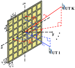
Figure 1: Illustration of the array geometry.

As illustrated in Figure 1, the UPA is placed on the $x$-$z$ plane and centered at the origin. We set $M=M_{x}M_{z}$, where $M_{x}$ and $M_{z}$ denote the number of array elements along the $x$- and $z$-axes, respectively. Without loss of generality, we assume that $M_{x}$ and $M_{z}$ are odd numbers with $M_{x}=2\tilde{M}_{x}+1$ and $M_{z}=2\tilde{M}_{z}+1$. The physical dimensions of each BS array element along the $x$- and $z$-axes are denoted by $\sqrt{A}$, and the inter-element distance is $d$, where $d\geq\sqrt{A}$. The central location of the $(m_{x},m_{z})$th element is denoted by ${\mathbf{s}}_{m_{x},m_{z}}=[m_{x}d,0,m_{z}d]^{\mathsf{T}}$, where $m_{x}\in{\mathcal{M}}_{x}\triangleq\{0,\pm 1,\ldots,\pm\tilde{M}_{x}\}$ and $m_{z}\in{\mathcal{M}}_{z}\triangleq\{0,\pm 1,\ldots,\pm\tilde{M}_{z}\}$.

Regarding each UT $k\in\mathcal{K}$, they are all assumed to be equipped with a single hypothetical isotropic array element to receive or transmit signals. Let $r_{k}$ denote the propagation distance from the center of the antenna array to UT $k$, and $\theta_{k}\in[0,\pi]$ and $\phi_{k}\in[0,\pi]$ denote the associated azimuth and elevation angles, respectively. Thus, the location of UT $k$ can be expressed as ${\mathbf{r}}_{k}=[r_{k}\Phi_{k},r_{k}\Psi_{k},r_{k}\Omega_{k}]^{\mathsf{T}}$, where $\Phi_{k}\triangleq\sin{\phi_{k}}\cos{\theta_{k}}$, $\Psi_{k}\triangleq\sin\phi_{k}\sin\theta_{k}$, and $\Omega_{k}\triangleq\cos{\phi_{k}}$. In particular, the distance between UT $k$ and the center of the $(m_{x},m_{z})$th array element is given by

$$r_{m_{x},m_{z},k}=\lVert{\mathbf{r}}_{k}-{\mathbf{s}}_{m_{x},m_{z}}\rVert$$

$$=r_{k}\sqrt{(m_{x}^{2}+m_{z}^{2})\epsilon_{k}^{2}-2m_{x}\epsilon_{k}\Phi_{k}-2m_{z}\epsilon_{k}\Omega_{k}+1},$$ (1)

where $\epsilon_{k}=\frac{d}{r_{k}}$. Note that $r_{k}=r_{0,0,k}$, and since the array element separation $d$ is typically on the order of a wavelength, in practice, we have $\epsilon_{k}\ll 1$.

II-A Channel Model

The channel response from UT $k$ to the $(m_{x},m_{z})$th antenna element of the BS is given by $h_{m_{x},m_{z},k}=\sqrt{g_{m_{x},m_{z},k}}\mathrm{e}^{-\mathrm{j}\phi_{m_{x},m_{z},k}}$, where

$$g_{m_{x},m_{z},k}=\int_{{\mathcal{S}}_{m_{x},m_{z}}}{\mathsf{g}}(\mathbf{r}_{k},{\mathbf{s}}){\frac{\lvert{\mathbf{e}}_{y}^{\mathsf{T}}({\mathbf{s}}-{\mathbf{r}}_{k})\rvert}{\lVert{\mathbf{r}}_{k}-{\mathbf{s}}\rVert}}{\rm{d}}{\mathbf{s}}.$$ (2)

Specifically, ${\mathcal{S}}_{m_{x},m_{z}}=[m_{x}d-{\sqrt{A}}/{2},m_{x}d+{\sqrt{A}}/{2}]\times[m_{z}d-{\sqrt{A}}/{2},m_{z}d+{\sqrt{A}}/{2}]$ denotes the aperture of the $(m_{x},m_{z})$th array element, and the term $\frac{\lvert{\mathbf{e}}_{y}^{\mathsf{T}}({\mathbf{s}}-{\mathbf{r}})\rvert}{\lVert{\mathbf{r}}-{\mathbf{s}}\rVert}$ captures the impact of the projected aperture of the UPA with ${\mathbf{e}}_{y}=[0,1,0]^{\mathsf{T}}$ being the UPA normal vector. Moreover, ${\mathsf{g}}(\mathbf{r},{\mathbf{s}})$ models the influence of free-space EM propagation, which is given by [1]

$${\mathsf{g}}(\mathbf{r},{\mathbf{s}})=\frac{1}{{4\pi}\lVert{\mathbf{r}}-{\mathbf{s}}\rVert^{2}}\bigg{(}1-\frac{1}{k_{0}^{2}\lVert{\mathbf{r}}-{\mathbf{s}}\rVert^{2}}+\frac{1}{k_{0}^{4}\lVert{\mathbf{r}}-{\mathbf{s}}\rVert^{4}}\bigg{)},$$ (3)

where $k_{0}=\frac{2\pi}{\lambda}$ is the wavenumber with $\lambda$ denoting the wavelength. Due to the small antenna size, i.e., $\sqrt{A}$, compared to the propagation distance between the user and antenna elements, i.e., $\lVert{\mathbf{r}}_{k}-{\mathbf{s}}_{m_{x},m_{z}}\rVert$, the variation of the channel response within an antenna element is negligible. This gives

$$g_{m_{x},m_{z},k}\approx A{\mathsf{g}}(\mathbf{r}_{k},{\mathbf{s}}_{m_{x},m_{z}})\frac{\lvert{\mathbf{e}}_{y}^{\mathsf{T}}({\mathbf{s}}_{m_{x},m_{z}}-{\mathbf{r}}_{k})\rvert}{\lVert{\mathbf{r}}_{k}-{\mathbf{s}}_{m_{x},m_{z}}\rVert}.$$ (4)

Furthermore, applying this approximation to the phase component, we obtain $\phi_{m_{x},m_{z},k}\approx\frac{2\pi}{\lambda}r_{m_{x},m_{z},k}$.

The function ${\mathsf{g}}(\mathbf{r},{\mathbf{s}})$ comprises three terms: the first term corresponds to the radiating NF and FF regions, while the remaining two terms correspond to the reactive NF region. Note that $1-\frac{1}{k_{0}^{2}\lVert{\mathbf{r}}-{\mathbf{s}}\rVert^{2}}+\frac{1}{k_{0}^{4}\lVert{\mathbf{r}}-{\mathbf{s}}\rVert^{4}}\approx 0.97$ at distance $\lVert{\mathbf{r}}-{\mathbf{s}}\rVert=\lambda$ [18]. Hence, when considering practical NFC systems with $r_{k}\gg\lambda$, the last two terms in (3) can be neglected. Consequently, the NF channel coefficient can be modeled as

$$h_{m_{x},m_{z},k}\approx\sqrt{\frac{Ar_{k}\Psi_{k}}{4\pi r_{m_{x},m_{z},k}^{3}}}\mathrm{e}^{-\mathrm{j}\frac{2\pi}{\lambda}r_{m_{x},m_{z},k}}.$$ (5)

For clarity, we denote $\mathbf{h}_{k}=[h_{m_{x},m_{z},k}]_{\forall m_{x},m_{z}}\in\mathbbmss{C}^{M\times 1}$ as the channel vector from UT $k$ to the BS.

For comparison, we also present the planar-wave based FF channel model. In contrast to the NF model, the FF model assumes that the angles of the links between each array element and UT $k$ are approximated to be identical, which results in linearly varying phase shifts. Additionally, variations in channel power across the BS array are considered negligible. Thus, the FF channel coefficient satisfies

$$h_{m_{x},m_{z},k}\approx\sqrt{\frac{A\Psi_{k}}{4\pi r_{k}^{2}}}\mathrm{e}^{-\mathrm{j}\frac{2\pi r_{k}}{\lambda}(1-m_{x}\epsilon_{k}\Phi_{k}-m_{z}\epsilon_{k}\Omega_{k})}.$$ (6)

Comparing (5) with (6) leads to the following observation.

Remark 1.

In contrast to FF channels, spherical wavefronts introduce additional range dimensions $\{r_{m_{x},m_{z},k}\}_{m_{x},m_{z}}$ to NF channels.

II-B Signal Models for Multiuser Communications

The system layout illustrated in Figure 1 establishes the foundational framework for multiuser NFC. We next refine this basic model into three models of significant research interest: MAC, BC, and MC. Throughout this paper, the channel is assumed to be known perfectly at the transceivers.

II-B1 MAC

MAC refers to the scenario where all UTs simultaneously send its own message to the BS. The received signal vector at the BS is given by

$${\mathbf{y}}=\sum\nolimits_{k=1}^{K}{\mathbf{h}_{k}x_{k}}+{\mathbf{n}},$$ (7)

where $x_{k}\in{\mathbbmss{C}}$ is the signal sent by UT $k$ with mean zero and variance ${\mathbbmss{E}}\{\lvert x_{k}\rvert^{2}\}\triangleq p_{k}$, and ${\mathbf{n}}\sim{\mathcal{CN}}({\mathbf{0}},\sigma^{2}{\mathbf{I}})$ is the additive white Gaussian noise (AWGN) with power $\sigma^{2}$.

II-B2 BC

If we reverse the MAC and have one BS broadcasting simultaneously to all UTs, it becomes the BC. The received signal at each UT $k$ is given by

$$y_{k}={\mathbf{h}}_{k}^{\mathsf{H}}{\mathbf{x}}+{{n}}_{k},$$ (8)

where ${\mathbf{x}}\in{\mathbbmss{C}}^{M\times 1}$ is the transmitted vector with mean zero and covariance matrix ${\mathbbmss{E}\{{\mathbf{x}}{\mathbf{x}}^{\mathsf{H}}\}}\triangleq{\bm{\Sigma}}$, and $n_{k}\sim{\mathcal{CN}}(0,\sigma_{k}^{2})$ is the AWGN with power $\sigma_{k}^{2}$. After receiving $y_{k}$, UT $k$ will exploit a decoder to recover the private message dedicated for himself from $y_{k}$.

II-B3 MC

MC refers to the scenario where the BS sends a common message to all UTs. In this case, the received signal at each UT $k$ can be still described as (8).

In the sequel, we will analyze the NF capacity of the above three channels, and compare them with their FF counterpart to gather insights. For clarity, the following analysis will focus on the two-user scenario, while certain findings can be extended to cases involving more than two UTs.

III Multiple Access Channel

In this section, we analyze the NF channel capacity of MAC by deriving its sum-rate capacity and capacity region.

III-A Sum-Rate Capacity

Given the power budget $P_{k}$ for UT $k$, the sum-rate capacity of the MAC can be written as follows:

$${\mathsf{C}}_{\mathsf{MAC}}=\max_{0\leq p_{k}\leq P_{k}}\log_{2}\det\left({\mathbf{I}}+\frac{1}{\sigma^{2}}\sum\nolimits_{k=1}^{K}{p_{k}}{\mathbf{h}}_{k}{\mathbf{h}}_{k}^{\mathsf{H}}\right),$$ (9)

which can be achieved by using point-to-point Gaussian random coding along with successive interference cancellation (SIC) decoding in some message decoding order [7]. From (9), it is readily shown that the sum-rate MAC capacity is attained when each UT transmits at the maximum power, i.e., $p_{k}=P_{k}$ for $k\in{\mathcal{K}}$, which yields

$${\mathsf{C}}_{\mathsf{MAC}}=\log_{2}\det\left({\mathbf{I}}+\frac{1}{\sigma^{2}}\sum\nolimits_{k=1}^{K}{P_{k}}{\mathbf{h}}_{k}{\mathbf{h}}_{k}^{\mathsf{H}}\right).$$ (10)

In the sequel, we derive a closed-form expression for ${\mathsf{C}}_{\mathsf{MAC}}$ by considering a two-user scenario, i.e., $K=2$, and the results will be further extended to the case of $K>2$ in Section III-D. By defining $\rho\triangleq\frac{\lvert{\mathbf{h}}_{1}^{\mathsf{H}}{\mathbf{h}}_{2}\rvert^{2}}{\lVert{\mathbf{h}}_{1}\rVert^{2}\lVert{\mathbf{h}}_{2}\rVert^{2}}\in[0,1]$ as the channel correlation factor (CCF), we obtain the following lemma.

Lemma 1.

The sum-rate capacity of the two-user MAC can be expressed as follows:

$$\begin{split}\mathsf{C}_{\mathsf{MAC}}&=\log_{2}(1+{\sigma^{-2}}({P_{1}\|\mathbf{h}_{1}\|^{2}+P_{2}\|\mathbf{h}_{2}\|^{2}})\\ &~{}~{}+{\sigma^{-4}}{P_{1}P_{2}\|\mathbf{h}_{1}\|^{2}\|\mathbf{h}_{2}\|^{2}}(1-\rho)).\end{split}$$ (11)

Proof:

Please refer to Appendix -A for more details. ∎

Remark 2.

The results in (11) suggest that the sum-rate capacity is influenced by the CCF between the two UTs, which reflects the impact of IUI. An ideal scenario occurs when the channels for the two UTs are orthogonal, which yields $\rho=0$ and indicates no IUI. This establishes an upper bound for $\mathsf{C}_{\mathsf{MAC}}$, which can be expressed as follows:

$$\mathsf{C}_{\mathsf{MAC}} \leq\log_{2}(1+{\sigma^{-2}}({P_{1}\|\mathbf{h}_{1}\|^{2}+P_{2}\|\mathbf{h}_{2}\|^{2}})$$

$$~{}~{}+{\sigma^{-4}}{P_{1}P_{2}\|\mathbf{h}_{1}\|^{2}\|\mathbf{h}_{2}\|^{2}})$$

$$=\sum\nolimits_{k=1}^{2}\log_{2}(1+{\sigma^{-2}}P_{k}\|\mathbf{h}_{k}\|^{2}).$$ (12)

By further incorporating the NF channel model (5) into the analysis, we derive the NF MAC capacity as follows.

Theorem 1.

The sum-rate capacity of the MAC under the NF model is given by

$${\mathsf{C}}_{\mathsf{MAC}}=\log_{2}\!\left(1\!+\frac{P_{1}G_{1}\!+\!P_{2}G_{2}}{\sigma^{2}}+\frac{P_{1}P_{2}G_{1}G_{2}\bar{\rho}}{\sigma^{4}}\right),$$ (13)

where $\bar{\rho}=1-\rho_{{}_{\mathsf{N}}}$. Specifically,

$$G_{k}=\frac{\xi}{4\pi}\sum\nolimits_{x\in\{\frac{M_{x}\epsilon_{k}}{2}\pm\Phi_{k}\}}{\sum\nolimits_{z\in\{\frac{M_{z}\epsilon_{k}}{2}\pm\Omega_{k}\}}{\delta_{k}\left(x,z\right)}}$$ (14)

denotes the channel gain of UT $k=1,2$. Furthermore,

$$\begin{split}\rho_{{}_{\mathsf{N}}}&=\prod\nolimits_{k=1}^{2}{\frac{d^{2}r_{k}\Psi_{k}}{\sum_{x\in\mathcal{X}_{k}}{\sum_{z\in\mathcal{Z}_{k}}{\delta_{k}\left(x,z\right)}}}}\\ &\times\left[\left(\sum\nolimits_{m_{x}\in\mathcal{M}_{x}}{\sum\nolimits_{m_{z}\in\mathcal{M}_{z}}{\Upsilon_{m_{x},m_{z}}^{-\frac{3}{2}}\cos\Delta_{m_{x},m_{z}}}}\right)^{2}\right.\\ &\left.+\left(\sum\nolimits_{m_{x}\in\mathcal{M}_{x}}{\sum\nolimits_{m_{z}\in\mathcal{M}_{z}}{\Upsilon_{m_{x},m_{z}}^{-\frac{3}{2}}\sin\Delta_{m_{x},m_{z}}}}\right)^{2}\right]\end{split}$$ (15)

denotes the CCF under the NF model, where $\Upsilon_{m_{x},m_{z}}=r_{m_{x},m_{z},1}r_{m_{x},m_{z},2}$, and $\Delta_{m_{x},m_{z}}=\frac{2\pi}{\lambda}\left(r_{m_{x},m_{z},1}-r_{m_{x},m_{z},2}\right)$.

Proof:

Please refer to Appendix -B for more details. ∎

We next aim to gain further insights into $\mathsf{C}_{\mathsf{MAC}}$ by considering an infinitely large array aperture. Specifically, when $M_{x},M_{z}\rightarrow\infty$, we have

$$\lim_{M_{x},M_{z}\rightarrow\infty}G_{k}=\frac{\xi}{4\pi}4\times\lim_{x,z\rightarrow\infty}\delta_{k}\left(x,z\right)=\frac{\xi}{2},$$ (16)

where $\xi=\frac{A}{d^{2}}\in\left(0,1\right]$ denotes the array occupation ratio (AOR) that measures the proportion of the entire UPA area occupied by antennas. Combining (12) with (16) gives

$$\lim_{M_{x},M_{z}\rightarrow\infty}\mathsf{C}_{\mathsf{MAC}}\leq\sum\nolimits_{k=1}^{2}\log_{2}(1+P_{k}\xi/(2\sigma^{2})),$$ (17)

which suggests that the NF MAC capacity is capped as $M_{x},M_{z}\rightarrow\infty$.

In contrast to $\lim_{M_{x},{M}_{z}\rightarrow\infty}G_{k}$, $\lim_{M_{x},{M}_{z}\rightarrow\infty}\rho_{{}_{\mathsf{N}}}$ is computationally intractable. However, numerical results presented in [19] demonstrate that $\lim_{M_{x},{M}_{z}\rightarrow\infty}\rho_{{}_{\mathsf{N}}}\ll 1$, which is also verified by the results in Section VI. This observation suggests that as the array aperture increases, NF channels of UTs positioned at different locations tend to become orthogonal, which presents an opportunity to mitigate IUI.

Corollary 1.

When $M_{x},M_{z}\rightarrow\infty$, the asymptotic NF MAC capacity is given by

$$\lim_{M_{x},M_{z}\rightarrow\infty}\mathsf{C}_{\mathsf{MAC}}\approx\sum\nolimits_{k=1}^{2}\log_{2}(1+P_{k}\xi/(2\sigma^{2})).$$ (18)

Proof:

Equation (18) is derived using (16) and the fact that $\lim_{M_{x},{M}_{z}\rightarrow\infty}\rho_{{}_{\mathsf{N}}}\ll 1$. ∎

Remark 3.

The results of Corollary 1 suggest that, as $M_{x},M_{z}\rightarrow\infty$, the NF MAC capacity converge to a finite value positively correlated to the AOR.

Remark 4.

The asymptotic NF MAC capacity closely approximates its upper bound presented in (17), as setting $M_{x},M_{z}\rightarrow\infty$ nearly removes the impact of IUI.

We then consider a special case where the BS uses a uniform linear array (ULA), i.e., $M_{x}=1$ and $M_{z}=M$.

Corollary 2.

When using a ULA, the channel gains satisfy

$$G_{k}=\frac{\xi\epsilon_{k}\sin\phi_{k}\Xi}{4\pi\sin\theta_{k}},$$ (19)

where $\Xi=\frac{M\epsilon_{k}-2\cos\theta_{k}}{\sqrt{M^{2}\epsilon_{k}^{2}-4M\cos\theta_{k}\epsilon_{k}+4}}+\frac{M\epsilon_{k}+2\cos\theta_{k}}{\sqrt{M^{2}\epsilon_{k}^{2}+4M\cos\theta_{k}\epsilon_{k}+4}}$. Accordingly, the MAC capacity satisfies

$$\lim_{M\rightarrow\infty}\!\mathsf{C}_{\mathsf{MAC}}\!\approx\log_{2} \!\left(\!1\!+\!\frac{P_{1}\epsilon_{1}\sin\phi_{1}\sin\theta_{2}\!+\!P_{2}\epsilon_{2}\sin\phi_{2}\sin\theta_{1}}{2\pi\sigma^{2}\sin\theta_{1}\sin\theta_{2}}\xi\right.$$

$$\left.+\frac{P_{1}P_{2}\epsilon_{1}\epsilon_{2}\sin\phi_{1}\sin\phi_{2}\xi^{2}}{4\pi^{2}\sigma^{4}\sin\theta_{1}\sin\theta_{2}}\right),$$ (20)

which is also a finite value.

Proof:

Please refer to Appendix -C for more details. ∎

III-B Capacity Region

Having obtained the sum-rate capacity, we now explore the capacity region. For a two-user NF MAC, its capacity region contains all the achievable rate pairs $({\mathsf{R}}_{1},{\mathsf{R}}_{2})$ such that [9]

$${\mathsf{R}}_{1}\leq\log_{2}(1+{P_{1}}{\sigma^{-2}}G_{1}),{\mathsf{R}}_{2}\leq\log_{2}(1+{P_{2}}{\sigma^{-2}}G_{2}),$$ (21a)

$${\mathsf{R}}_{1}+{\mathsf{R}}_{2}\leq{\mathsf{C}}_{\mathsf{MAC}},$$ (21b)

where ${\mathsf{R}}_{k}$ denotes the achievable rate of UT $k=1,2$. The MAC capacity region forms a pentagon, with its corner points attained through SIC decoding, and the line segment connecting these points achieved through time sharing, as seen in [7, Figure 7]. The corner points are computed as follows.

Lemma 2.

When the SIC decoding order $1\rightarrow 2$ is adopted, the rates of the two UTs are, respectively, given by

$${\mathsf{R}}_{1}^{1\rightarrow 2}=\log_{2}\!\left(1+\frac{P_{1}\sigma^{-2}G_{1}+P_{1}P_{2}\sigma^{-4}G_{1}G_{2}\bar{\rho}}{1+P_{2}\sigma^{-2}G_{2}}\right),$$ (22a)

$${\mathsf{R}}_{2}^{1\rightarrow 2}=\log_{2}\left(1+P_{2}\sigma^{-2}G_{2}\right).$$ (22b)

For the decoding order $2\rightarrow 1$, we have

$${\mathsf{R}}_{1}^{2\rightarrow 1}=\log_{2}\left(1+P_{1}\sigma^{-2}G_{1}\right),$$ (23a)

$${\mathsf{R}}_{2}^{2\rightarrow 1}=\log_{2}\left(1+\frac{P_{2}\sigma^{-2}G_{2}+P_{1}P_{2}\sigma^{-4}G_{1}G_{2}\bar{\rho}}{1+P_{1}\sigma^{-2}G_{1}}\right).$$ (23b)

Proof:

Please refer to Appendix -D for more details. ∎

Regarding time sharing, it means that applying the SIC order $1\rightarrow 2$ with probability $\tau$, while applying $2\rightarrow 1$ with probability $1-\tau$, where $\tau\in(0,1)$. Given $\tau$, by denoting the achievable rate pair as $({\mathsf{R}}_{1}^{\tau},{\mathsf{R}}_{2}^{\tau})$, we have ${\mathsf{R}}_{1}^{\tau}=\tau{\mathsf{R}}_{1}^{1\rightarrow 2}+(1-\tau){\mathsf{R}}_{1}^{2\rightarrow 1}$ and ${\mathsf{R}}_{2}^{\tau}=\tau{\mathsf{R}}_{2}^{1\rightarrow 2}+(1-\tau){\mathsf{R}}_{2}^{2\rightarrow 1}$. As a result, the MAC capacity region is given by

$$\!\mathcal{R}_{\mathsf{MAC}}\!=\!\left\{({\mathsf{R}}_{1},{\mathsf{R}}_{2})\left|{\mathsf{R}}_{1}\!\in\!\left[0,{\mathsf{R}}_{1}^{\tau}\right],{\mathsf{R}}_{2}\!\in\![0,{\mathsf{R}}_{2}^{\tau}],\tau\!\in\![0,1]\right.\!\right\}.$$ (24)

Next, we consider the case where $M_{x},M_{z}\rightarrow\infty$.

Corollary 3.

When $M_{x},M_{z}\rightarrow\infty$, the corner points of the MAC capacity region satisfy

$$\begin{split}&\lim_{M_{x},M_{z}\rightarrow\infty}(\mathsf{R}_{1}^{1\rightarrow 2},\mathsf{R}_{2}^{1\rightarrow 2})\approx\lim_{M_{x},M_{z}\rightarrow\infty}(\mathsf{R}_{1}^{2\rightarrow 1},\mathsf{R}_{2}^{2\rightarrow 1})\\ &~{}~{}~{}\approx\left(\log_{2}(1+{P_{1}\xi}/{(2\sigma^{2})}),\log_{2}(1+{P_{2}\xi}/{(2\sigma^{2})})\right).\end{split}$$ (25)

Proof:

Similar to the proof of Corollary 1. ∎

Remark 5.

The findings in Corollary 3 indicate that as the number of antennas increases, the two corner points tend to approach each other. This causes the NF MAC capacity region to transition from a pentagon to a finite rectangle, implying that the rates are no longer influenced by the SIC order.

III-C Comparison with the FF Capacity

We now focus on the FF case for comparison.

Proposition 1.

Under the FF model, the channel gains are given by $G_{k}^{\mathsf{F}}=\frac{MA\Psi_{k}}{4\pi r_{k}^{2}}$ for $k=1,2$, and the CCF satisfies

$$\rho_{{}_{\mathsf{F}}}=\left\{\!\begin{array}[]{ll}1&\left(\theta_{1},\phi_{1}\right)\!=\!\left(\theta_{2},\phi_{2}\right)\\ \frac{1-\cos\left(M_{x}\Delta_{\Phi}\right)}{M^{2}\left(1-\cos\Delta_{\Phi}\right)}&\Phi_{1}\!\neq\!\Phi_{2},\Omega_{1}\!=\!\Omega_{2}\\ \frac{1-\cos\left(M_{z}\Delta_{\Omega}\right)}{M^{2}\left(1-\cos\Delta_{\Omega}\right)}&\Phi_{1}\!=\!\Phi_{2},\Omega_{1}\!\neq\!\Omega_{2}\\ \frac{4\left(1-\cos\left(M_{x}\Delta_{\Phi}\right)\right)\left(1-\cos\left(M_{z}\Delta_{\Omega}\right)\right)}{M^{2}\left(1-\cos\Delta_{\Phi}\right)\left(1-\cos\Delta_{\Omega}\right)}&\text{else}\\ \end{array}\right.,$$ (30)

where $\Delta_{\Phi}=\frac{2\pi}{\lambda}d\left(\Phi_{1}-\Phi_{2}\right)$, and $\Delta_{\Omega}=\frac{2\pi}{\lambda}d\left(\Omega_{1}-\Omega_{2}\right)$.

Proof:

Please refer to Appendix -E. ∎

Using Proposition 1, the closed-form expressions for the FF MAC capacity and the capacity region follow immediately, which are omitted due to space limitations.

Corollary 4.

Under the FF model, when $M\rightarrow\infty$, the asymptotic MAC capacity is given in (31), shown at the bottom of this page, which yields $\mathsf{C}_{\mathsf{MAC}}^{\mathsf{F}}\simeq\mathcal{O}\left(\log M\right)$.

Proof:

The results can be obtained using the fact that $\lim_{M\rightarrow\infty}\rho_{{}_{\mathsf{F}}}=\begin{cases}1&\left(\theta_{1},\phi_{1}\right)=\left(\theta_{2},\phi_{2}\right)\\ 0&\left(\theta_{1},\phi_{1}\right)\neq\left(\theta_{2},\phi_{2}\right)\\ \end{cases}$, along with the approximation $\log_{2}(1+x)\approx\log_{2}x$ for large $x$. ∎

$$\mathsf{C}_{\mathsf{MAC}}^{\mathsf{F}}\simeq\begin{cases}\log_{2}\left(\frac{MA}{4\pi\sigma^{2}}\left(\frac{P_{1}\Psi_{1}}{r_{1}^{2}}+\frac{P_{2}\Psi_{2}}{r_{2}^{2}}\right)\right)\triangleq\mathsf{F}_{\mathsf{MAC}}^{\mathsf{s}}&\left(\theta_{1},\phi_{1}\right)=\left(\theta_{2},\phi_{2}\right)\\ \log_{2}\left(\frac{MA}{4\pi\sigma^{2}}\left(\frac{P_{1}\Psi_{1}}{r_{1}^{2}}+\frac{P_{2}\Psi_{2}}{r_{2}^{2}}\right)+\frac{M^{2}A^{2}P_{1}P_{2}\Psi_{1}\Psi_{2}}{16\pi^{2}r_{1}^{2}r_{2}^{2}\sigma^{4}}\right)\triangleq\mathsf{F}_{\mathsf{MAC}}^{\mathsf{d}}&\left(\theta_{1},\phi_{1}\right)\neq\left(\theta_{2},\phi_{2}\right)\\ \end{cases}$$ (31)

$$\mathsf{F}_{\mathsf{MAC}}^{\mathsf{d}}-\mathsf{F}_{\mathsf{MAC}}^{\mathsf{s}}=\log_{2}\left(1+\frac{MA}{4\pi\left(P_{1}^{-1}\Psi_{1}^{-1}r_{1}^{2}+P_{2}^{-1}\Psi_{2}^{-1}r_{2}^{2}\right)\sigma^{2}}\right)>0$$ (32)

Remark 6.

Rather than converging to a finite bound as under the NF model, the FF MAC sum-rate capacity grows unboundedly with the number of the BS antennas, theoretically achieving any desired level, which poses a contradiction to the energy-conservation laws.

This contradiction stems from the assumption of uniform channel power across each antenna element, which becomes increasingly inaccurate as the number of the elements grows. Furthermore, comparing the FF MAC capacity for co-directional UTs and UTs with differing directions, as indicated in (32) below, yields the following observation.

Remark 7.

The FF MAC capacity significantly diminishes when UTs are oriented in the same direction compared to cases where they face different directions. This contrast with the NF model arises from the high channel correlation ($\rho_{{}_{\mathsf{F}}}=1$) among UTs in the same direction, leading to notable IUI.

By letting $M\rightarrow\infty$, we characterize the FF MAC capacity region as follows.

Corollary 5.

Under the FF model, when $M\rightarrow\infty$, if UTs are in the same direction, the corner points approximately satisfy $(\mathsf{R}_{1}^{1\rightarrow 2},\mathsf{R}_{2}^{1\rightarrow 2})\simeq(\log_{2}(1+\frac{P_{1}r_{2}^{2}}{P_{2}r_{1}^{2}}),\mathcal{O}(\log M))$ and $(\mathsf{R}_{1}^{2\rightarrow 1},\mathsf{R}_{2}^{2\rightarrow 1})\simeq(\mathcal{O}(\log M),\log_{2}(1+\frac{P_{2}r_{1}^{2}}{P_{1}r_{2}^{2}}))$. If UTs are positioned in different directions, $(\mathsf{R}_{1}^{1\rightarrow 2},\mathsf{R}_{2}^{1\rightarrow 2})\simeq(\mathsf{R}_{1}^{2\rightarrow 1},\mathsf{R}_{2}^{2\rightarrow 1})\simeq\left(\mathcal{O}\left(\log M\right),\mathcal{O}\left(\log M\right)\right)$.

Proof:

Similar to the proof of Corollary 4. ∎

Remark 8.

The results in Corollary 5 indicate that the MAC capacity region under the FF model can expand unboundedly with the number of array elements, rendering it impractical.

Remark 9.

When UTs face different directions, the FF MAC capacity region roughly forms a rectangle and is more extensive than that when UTs are in the same direction.

By comparing the NF capacity with its FF counterpart, we draw the following conclusions:

• The adoption of the FF channel model for a large antenna array may lead to outcomes that conflict with the fundamental principle of energy conservation. This issue arises because the NF region expands as the array size increases, which challenges the FF assumption of uniform plane-wave propagation. On the other hand, the NF model is more sustainable under energy considerations. The above facts underscore the necessity for channel modeling within the NF region using spherical-wave propagation to capture the physical reality more accurately.

• Different from the FF MAC capacity that degenerates for co-directional UTs due to the significant IUI, the NF capacity can be preserved when UTs are located at different locations (different directions or distances), which underscores superior flexibility and robust interference management capabilities inherent to NFC. This additional resolution in the range domain enable space-division multiple access [20] from FF angle-division multiple access to NF range-division multiple access, demonstrating the NFC’s potential as a promising approach for efficient and interference-free communication systems.

III-D Extension to Cases of $K>2$

The sum-rate capacity of the MAC for $K>2$ is given by

$${\mathsf{C}}_{\mathsf{MAC}}=\log_{2}\det\Big{(}{\mathbf{I}}+{\sigma^{-2}}\sum\nolimits_{k=1}^{K}{P_{k}}{\mathbf{h}}_{k}{\mathbf{h}}_{k}^{\mathsf{H}}\Big{)}.$$ (33)

Following steps similar to those in Appendix -A, (33) can be rewritten as $\mathsf{C}_{\mathsf{MAC}}=\log_{2}\det\left(\mathbf{A}\right)$ with

$$\mathbf{A}=\left[\begin{matrix}1+\frac{P_{1}}{\sigma^{2}}\|\mathbf{h}_{1}\|^{2}&\cdots&1+\frac{\sqrt{P_{1}P_{K}}}{\sigma^{2}}\mathbf{h}_{1}^{\mathsf{H}}\mathbf{h}_{K}\\ \vdots&\ddots&\vdots\\ 1+\frac{\sqrt{P_{1}P_{K}}}{\sigma^{2}}\mathbf{h}_{K}^{\mathsf{H}}\mathbf{h}_{1}&\cdots&1+\frac{P_{K}}{\sigma^{2}}\|\mathbf{h}_{K}\|^{2}\\ \end{matrix}\right],$$ (34)

which can be expressed in terms of a function of the channel gains and CCFs.

The capacity region of the MAC exhibits a polymatroidal structure in $K$-dimensional space, and each of the $K!$ corner points can be attained by employing SIC decoding in a specific message decoding order. The remaining capacity region is realized through time-sharing among these corner points. Specifically, when considering the SIC decoding order $\varpi(K)\rightarrow\varpi(K-1)\rightarrow\ldots\rightarrow\varpi(1)$ with $\{\varpi(k)\}_{k=1}^{K}={\mathcal{K}}$, the achievable rate tuple $({\mathsf{R}}_{1},\ldots,{\mathsf{R}}_{K})$ at each corner point of the capacity region can be calculated as

$$\begin{split}&\mathsf{R}_{\varpi\left(k\right)}=\log_{2}\left(1+{P_{\varpi(k)}}{\sigma^{-2}}\|\mathbf{h}_{\varpi(k)}\|^{2}+\right.\\ &\times\left.\frac{P_{1}P_{2}\sigma^{-4}\sum\nolimits_{k^{\prime}<k}{P_{\varpi(k)}P_{\varpi(k^{\prime})}|\mathbf{h}_{\varpi(k)}^{\mathsf{H}}\mathbf{h}_{\varpi(k^{\prime})}|^{2}}}{1+\sigma^{-2}\sum\nolimits_{k^{\prime}<k}{P_{\varpi(k^{\prime})}\|\mathbf{h}_{\varpi(k^{\prime})}\|^{2}}}\right),\end{split}$$ (35)

which is also a function of the channel gains and CCFs. Therefore, the results derived in the case of $K=2$ can be trivially extended to the case of $K>2$.

IV Broadcast Channel

In this section, we investigate the sum-rate capacity and the capacity region of the BC.

IV-A Sum-Rate Capacity

The capacity of the multiantenna Gaussian BC is achieved by successive dirty-paper encoding with Gaussian codebooks [21, 11]. Let ${\bm{\Sigma}}_{k}\in{\mathbbmss{C}}^{M\times M}$ denote the covariance matrix in generating the dirty-paper Gaussian codebook for UT $k$. The transmitted signal is subject to the power budget ${\mathsf{tr}}({\bm{\Sigma}})=\sum_{k=1}^{K}{\mathsf{tr}}({\bm{\Sigma}}_{k})\leq P$. Without loss of generality, we consider the encoding order $\varepsilon(K)\rightarrow\varepsilon(K-1)\rightarrow\ldots\rightarrow\varepsilon(1)$ with $\{\varepsilon(k)\}_{k=1}^{K}={\mathcal{K}}$. Concerning UT $\varepsilon(k)$, the dirty-paper encoder considers the interference signal caused by UTs $\varepsilon(k^{\prime})$ for $k^{\prime}>k$ as known non-causally and his decoder treats the interference signal caused by UTs $\varepsilon(k^{\prime})$ for $k^{\prime}<k$ as additional noise. By applying dirty-paper coding and by using minimum Euclidean distance decoding at each UT, it follows that the achieved rate of UT $\varepsilon(k)$ is given by [22, 23]

$${\mathsf{R}}_{\varepsilon(k)}=\log_{2}\left(1\!+\!\frac{{\mathbf{h}}_{\varepsilon(k)}^{\mathsf{H}}{\bm{\Sigma}}_{\varepsilon(k)}{\mathbf{h}}_{\varepsilon(k)}}{\sigma_{\varepsilon(k)}^{2}\!+\!\sum_{k^{\prime}<k}{\mathbf{h}}_{\varepsilon(k^{\prime})}^{\mathsf{H}}{\bm{\Sigma}}_{\varepsilon(k^{\prime})}{\mathbf{h}}_{\varepsilon(k^{\prime})}}\right).$$ (36)

Consequently, the sum-rate capacity can be written in terms of the following maximization:

$${\mathsf{C}}_{\mathsf{BC}}=\max_{\{{\bm{\Sigma}}_{k}\}_{k=1}^{K}:{\bm{\Sigma}}_{k}\succeq{\mathbf{0}},\sum_{k=1}^{K}{\mathsf{tr}}({\bm{\Sigma}}_{k})\leq P}\sum\nolimits_{k=1}^{K}{{\mathsf{R}}_{\varepsilon(k)}}.$$ (37)

Based on (37), the sum-rate capacity of BS with two UTs is written as follows:

$${\mathsf{C}}_{\mathsf{BC}}= \max_{\{{\bm{\Sigma}}_{k}\}_{k=1}^{2}:{\bm{\Sigma}}_{k}\succeq{\mathbf{0}},\sum_{k=1}^{2}{\mathsf{tr}}({\bm{\Sigma}}_{k})\leq P}\log_{2}\left(1+\frac{{\mathbf{h}}_{1}^{\mathsf{H}}{\bm{\Sigma}}_{1}{\mathbf{h}}_{1}}{\sigma_{1}^{2}}\right)$$

$$\qquad\qquad\qquad+\log_{2}\left(1+\frac{{\mathbf{h}}_{2}^{\mathsf{H}}{\bm{\Sigma}}_{2}{\mathbf{h}}_{2}}{\sigma_{2}^{2}+{\mathbf{h}}_{2}^{\mathsf{H}}{\bm{\Sigma}}_{1}{\mathbf{h}}_{2}}\right).$$ (38)

The above expression is derived under the encoding order $2\rightarrow 1$. However, as indicated in [22, 23], the capacity is always the same regardless of the encoding order.

Problem (IV-A) is a non-convex problem. Thus, numerically finding the maximum is a nontrivial problem. However, in [22], a duality is shown to exist between the uplink and downlink which establishes that the dirty-paper capacity region for the BC is equal to the capacity region of the dual MAC (described in (7)). Therefore, (IV-A) can be rewritten as

$$\!{\mathsf{C}}_{\mathsf{BC}} =\max_{0\leq p_{k},\sum_{k=1}^{2}p_{k}=P}\log_{2}\det\left({\mathbf{I}}+\sum\nolimits_{k=1}^{K}\frac{p_{k}}{\sigma_{k}^{2}}{\mathbf{h}}_{k}{\mathbf{h}}_{k}^{\mathsf{H}}\right)$$

$$\!\!\!=\max_{0\leq p_{k},\sum_{k=1}^{2}p_{k}=P}\!\log_{2}\!\left(1\!+\frac{p_{1}}{\sigma_{1}^{2}}\left\|\mathbf{h}_{1}\right\|^{2}\!+\frac{p_{2}}{\sigma_{2}^{2}}\left\|\mathbf{h}_{2}\right\|^{2}\right.$$

$$\qquad\qquad\qquad\quad\left.+\frac{p_{1}p_{2}}{\sigma_{1}^{2}\sigma_{2}^{2}}\left\|\mathbf{h}_{1}\right\|^{2}\left\|\mathbf{h}_{2}\right\|^{2}\left(1-\rho\right)\right).$$ (39)

Note that problem (IV-A) is a convex problem which can be optimally solved. After obtaining the optimized $\{p_{k}\}_{k=1}^{2}$, we can employ the encoding order as well as the transformation in [22, Equs. (8)–(10)] and [23, Appendix A] to recover the corresponding downlink covariance matrices that achieve the same rates and the sum-rate.

Theorem 2.

The optimal power allocation in the NF scenario is given by

$$\left(p_{1}^{\star},p_{2}^{\star}\right)=\begin{cases}\left(P,0\right)&\kappa_{1}\leq 0\\ \left(0,P\right)&\kappa_{2}\leq 0\\ \left(\frac{\kappa_{1}\sigma_{2}^{2}}{G_{2}\bar{\rho}},\frac{\kappa_{2}\sigma_{1}^{2}}{G_{1}\bar{\rho}}\right)&\mathrm{else}\\ \end{cases},$$ (40)

where $\kappa_{1}=\frac{P\sigma_{1}^{-2}\sigma_{2}^{-2}G_{1}G_{2}\bar{\rho}-\sigma_{1}^{-2}G_{1}+\sigma_{2}^{-2}G_{2}}{2\sigma_{1}^{-2}G_{1}}$, and $\kappa_{2}=\frac{P\sigma_{1}^{-2}\sigma_{2}^{-2}G_{1}G_{2}\bar{\rho}+\sigma_{1}^{-2}G_{1}-\sigma_{2}^{-2}G_{2}}{2\sigma_{2}^{-2}G_{2}}$. Accordingly, the NF sum-rate capacity of the BC is given by

$$\mathsf{C}_{\mathsf{BC}}=\begin{cases}\log_{2}\big{(}1+P\sigma_{1}^{-2}G_{1}\big{)}&\kappa_{1}\leq 0\\ \log_{2}\big{(}1+P\sigma_{2}^{-2}G_{2}\big{)}&\kappa_{2}\leq 0\\ \log_{2}\big{(}1+\frac{\kappa_{1}+\kappa_{2}+\kappa_{1}\kappa_{2}}{\bar{\rho}}\big{)}&\text{else}\\ \end{cases}.$$ (41)

Proof:

The results can be obtained based on the Karush–Kuhn–Tucker (KKT) conditions of problem (IV-A). ∎

Corollary 6.

When $M_{x},M_{z}\rightarrow\infty$, the optimal power allocation policy degenerates into

$$\lim_{M_{x},M_{z}\rightarrow\infty}\left(p_{1}^{\star},p_{2}^{\star}\right)=\begin{cases}\left(P,0\right)&\tilde{\kappa}_{1}\leq 0\\ \left(0,P\right)&\tilde{\kappa}_{2}\leq 0\\ \left(\frac{2\tilde{\kappa}_{1}}{\sigma_{2}^{-2}\xi},\frac{2\tilde{\kappa}_{2}}{\sigma_{1}^{-2}\xi}\right)&\mathrm{else}\\ \end{cases},$$ (42)

where $\tilde{\kappa}_{1}=\frac{P\sigma_{1}^{-2}\sigma_{2}^{-2}\frac{\xi}{2}-\sigma_{1}^{-2}+\sigma_{2}^{-2}}{2\sigma_{1}^{-2}}$, and $\tilde{\kappa}_{2}=\frac{P\sigma_{1}^{-2}\sigma_{2}^{-2}\frac{\xi}{2}+\sigma_{1}^{-2}-\sigma_{2}^{-2}}{2\sigma_{2}^{-2}}$. Accordingly, the asymptotic BC capacity under the NF model is given by

$$\!\lim_{M_{x},M_{z}\rightarrow\infty}\mathsf{C}_{\mathsf{BC}}\approx\!\begin{cases}\log_{2}\left(1\!+\!\frac{P\xi}{2\sigma_{1}^{2}}\right)&\!\tilde{\kappa}_{1}\leq 0\\ \log_{2}\left(1\!+\!\frac{P\xi}{2\sigma_{2}^{2}}\right)&\!\tilde{\kappa}_{2}\leq 0\\ \log_{2}\left(1\!+\!\tilde{\kappa}_{1}\!+\!\tilde{\kappa}_{2}\!+\!\tilde{\kappa}_{1}\tilde{\kappa}_{2}\right)&\mathrm{else}\\ \end{cases}.$$ (43)

Proof:

Similar to the proof of Corollary 1. ∎

Remark 10.

The results in Corollary 6 suggest that, as $M_{x},M_{z}\rightarrow\infty$, the NF BC capacity converge to a finite value positively correlated to the AOR.

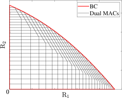
Figure 2: Illustration of the BC and dual MAC capacity regions.

Next, we consider the ULA case.

Corollary 7.

When the BS is equipped with a ULA, we have

$$\lim_{M\rightarrow\infty}\left(p_{1}^{\star},p_{2}^{\star}\right)=\begin{cases}\left(P,0\right)&\tilde{\kappa}_{1}^{\prime}\leq 0\\ \left(0,P\right)&\tilde{\kappa}_{2}^{\prime}\leq 0\\ \left(\frac{2\pi\tilde{\kappa}_{1}^{\prime}}{\nu_{2}\xi},\frac{2\pi\tilde{\kappa}_{1}^{\prime}}{\nu_{1}\xi}\right)&\mathrm{else}\\ \end{cases},$$ (44)

where $\nu_{1}=\sigma_{1}^{-2}\epsilon_{1}\sin\phi_{1}\sin\theta_{1}^{-1}$, $\nu_{2}=\sigma_{2}^{-2}\epsilon_{2}\sin\phi_{2}\sin\theta_{2}^{-1}$, $\tilde{\kappa}_{1}^{\prime}=\frac{\xi\left(2\pi\right)^{-1}P\nu_{1}\nu_{2}-\nu_{1}+\nu_{2}}{2\nu_{1}}$, and $\tilde{\kappa}_{2}^{\prime}=\frac{\xi\left(2\pi\right)^{-1}P\nu_{1}\nu_{2}+\nu_{1}-\nu_{2}}{2\nu_{2}}$. Subsequently, the sum-rate capacity satisfies

$$\lim_{M\rightarrow\infty}\mathsf{C}_{\mathsf{BC}}=\begin{cases}\log_{2}\left(1+\frac{P\nu_{1}\xi}{2\pi}\right)&\tilde{\kappa}_{1}^{\prime}\leq 0\\ \log_{2}\left(1+\frac{P\nu_{2}\xi}{2\pi}\right)&\tilde{\kappa}_{2}^{\prime}\leq 0\\ \log_{2}\left(1+\tilde{\kappa}_{1}^{\prime}+\tilde{\kappa}_{2}^{\prime}+\tilde{\kappa}_{1}^{\prime}\tilde{\kappa}_{2}^{\prime}\right)&\mathrm{else}\\ \end{cases},$$ (45)

which is a finite value.

Proof:

Similar to the proof of Corollary 2. ∎

Notably, if the noise power at each UTs is same, for the UPA case, we can deduce that $\lim_{M_{x},M_{z}\rightarrow\infty}\left(p_{1}^{\star},p_{2}^{\star}\right)=\left(\frac{P}{2},\frac{P}{2}\right)$, which indicates that the optimal power allocation strategy tends to an equal power allocation when the number of array element becomes extremely large. On the other hand, in the ULA scenario, the optimal power allocation always depends on the UT’s positions even when $M\rightarrow\infty$.

IV-B Capacity Region

Given a power allocation scheme $\{p_{k}\}_{k=1}^{2}$ with $p_{1}+p_{2}=P$, we can obtain the capacity region of a dual MAC. The capacity region of the BC is the convex hull of all these dual MAC capacity regions [22], which means that the boundary of capacity region of the BC is formed by the corner points of the dual MAC capacity regions, as illustrated in Fig 2. For a given power allocation scheme $\{p_{k}\}_{k=1}^{2}$, the two corner points of the capacity region of the dual MAC, $(\hat{\mathsf{R}}_{1}^{1\rightarrow 2},\hat{\mathsf{R}}_{2}^{1\rightarrow 2})$ and $(\hat{\mathsf{R}}_{1}^{2\rightarrow 1},\hat{\mathsf{R}}_{2}^{2\rightarrow 1})$, are given as follows. When the dirty-paper encoding order is $2\rightarrow 1$, we have

$$\hat{\mathsf{R}}_{1}^{1\rightarrow 2}\!=\log_{2}\!\Big{(}1\!+\frac{p_{1}\sigma_{1}^{-2}G_{1}\!+\!p_{1}p_{2}\sigma_{1}^{-2}\sigma_{2}^{-2}G_{1}G_{2}\bar{\rho}}{1+p_{2}\sigma_{2}^{-2}G_{2}}\Big{)},$$ (46a)

$$\hat{\mathsf{R}}_{2}^{1\rightarrow 2}=\log_{2}\left(1+p_{2}\sigma_{2}^{-2}G_{2}\right).$$ (46b)

When the dirty-paper encoding order is $1\rightarrow 2$, we have

$$\hat{\mathsf{R}}_{1}^{2\rightarrow 1}=\log_{2}\left(1+p_{1}\sigma_{1}^{-2}G_{1}\right),$$ (47a)

$$\hat{\mathsf{R}}_{2}^{2\rightarrow 1}\!=\log_{2}\!\Big{(}1\!+\frac{p_{2}\sigma_{2}^{-2}G_{2}\!+\!p_{1}p_{2}\sigma_{1}^{-2}\sigma_{2}^{-2}G_{1}G_{2}\bar{\rho}}{1+p_{1}\sigma_{1}^{-2}G_{1}}\Big{)}.$$ (47b)

For any given power allocation scheme $\{p_{k}\}_{k=1}^{2}$ with $p_{1}+p_{2}=P$, we can obtain the closed-form expressions for the corner points of the dual MAC regions. The BC capacity region can be then characterized by the convex hull of these corner points.

Corollary 8.

When $M_{x},M_{z}\rightarrow\infty$, the corner points of the dual MAC capacity region with a given power allocation $\{p_{k}\}_{k=1}^{2}$ satisfy

$$\lim_{M_{x},M_{z}\rightarrow\infty}\left(\hat{\mathsf{R}}_{1}^{1\rightarrow 2},\hat{\mathsf{R}}_{2}^{1\rightarrow 2}\right)\approx\lim_{M_{x},M_{z}\rightarrow\infty}\left(\hat{\mathsf{R}}_{1}^{2\rightarrow 1},\hat{\mathsf{R}}_{2}^{2\rightarrow 1}\right)$$

$$~{}~{}~{}\approx\left(\log_{2}(1+{p_{1}\xi}/{(2\sigma_{1}^{2})}),\log_{2}(1+{p_{2}\xi}/{(2\sigma_{2}^{2})})\right).$$ (48)

Proof:

Similar to the proof of Corollary 1. ∎

Remark 11.

The results in Corollary 8 suggest that, as the number of the array elements increases, the dual MAC capacity region approaches a finite rectangle, which implies that the NF capacity region of the BC is bounded.

IV-C Comparison with the FF Capacity

The FF BC capacity is given as follows.

Corollary 9.

For the FF case, the asymptotic BC capacity for $M\rightarrow\infty$ is given in (49), shown at the bottom of the next page, which yields $\mathsf{C}_{\mathsf{BC}}^{\mathsf{F}}\simeq\mathcal{O}(\log M)$.

Proof:

Similar to the proof of Corollary 4. ∎

Remark 12.

Rather than converging to a finite value as under the NF model, the BC sum-rate capacity under the FF model grows unboundedly with the number of the array elements, which potentially violates the energy-conservation laws.

According to the results of (50) below, we obtain the following remarks.

Remark 13.

In contrast to the NF case, the FF BC capacity with co-directional UTs is smaller than that when the UTs are in different directions.

The capacity region of the BC under the FF model, when considering an infinitely large array, is influenced by the relative directions of the UTs.

Corollary 10.

In the FF scenario, when $M\rightarrow\infty$, if the UTs are located in the same direction, the corner points of the dual MAC capacity region satisfy $(\hat{\mathsf{R}}_{1}^{1\rightarrow 2},\hat{\mathsf{R}}_{2}^{1\rightarrow 2})\simeq(\log_{2}(1\!+\frac{p_{1}r_{2}^{2}\sigma_{2}^{2}}{p_{2}r_{1}^{2}\sigma_{1}^{2}}),\mathcal{O}(\log M))$ and $(\hat{\mathsf{R}}_{1}^{2\rightarrow 1},\hat{\mathsf{R}}_{2}^{2\rightarrow 1})\simeq(\mathcal{O}(\log M),\log_{2}(1+\frac{p_{2}r_{1}^{2}\sigma_{1}^{2}}{p_{1}r_{2}^{2}\sigma_{2}^{2}}))$. If the UTs are positioned in different directions, we have $(\hat{\mathsf{R}}_{1}^{1\rightarrow 2},\hat{\mathsf{R}}_{2}^{1\rightarrow 2})\simeq(\hat{\mathsf{R}}_{1}^{2\rightarrow 1},\hat{\mathsf{R}}_{2}^{2\rightarrow 1})\simeq(\mathcal{O}(\log M),\mathcal{O}(\log M))$.

Proof:

Similar to the proof of Corollary 4. ∎

Remark 14.

The results in Corollary 10 suggest that the BC capacity region under the FF model can extend unboundedly with the number of the array elements, which is impractical.

Remark 15.

The FF BC capacity region of cases when the UTs are in different directions is more extensive than that of cases when the UTs are in a same direction.

The comparison between BC capacity under the NF and FF models, similar to the MAC, highlights the importance of incorporating NF modeling in asymptotic evaluations, which provides a more accurate and feasible framework in terms of energy sustainability. Additionally, the introduction of range dimensions by spherical-wave propagation in the NF model enhances the BC capacity for co-directional UTs.

$$\mathsf{C}_{\mathsf{BC}}^{\mathsf{F}}\simeq\begin{cases}\log_{2}\!\left(\frac{MPA}{4\pi}\max_{k=1,2}\frac{\Psi_{k}}{r_{k}^{2}\sigma_{k}^{2}}\right)\triangleq\mathsf{F}_{\mathsf{BC}}^{\mathsf{s}}&\left(\theta_{1},\phi_{1}\right)=\left(\theta_{2},\phi_{2}\right)\\ \log_{2}\left(\frac{\left(MPA\left(4\pi\right)^{-1}+\Psi_{1}^{-1}r_{1}^{2}\sigma_{1}^{2}+\Psi_{2}^{-1}r_{2}^{2}\sigma_{2}^{2}\right)^{2}}{4\Psi_{1}^{-1}\Psi_{2}^{-1}r_{1}^{2}r_{2}^{2}\sigma_{1}^{2}\sigma_{2}^{2}}-1\right)\triangleq\mathsf{F}_{\mathsf{BC}}^{\mathsf{d}}&\left(\theta_{1},\phi_{1}\right)\neq\left(\theta_{2},\phi_{2}\right)\\ \end{cases}$$ (49)

$$\mathsf{F}_{\mathsf{BC}}^{\mathsf{d}}-\mathsf{F}_{\mathsf{BC}}^{\mathsf{s}}=\log_{2}\left(1+\frac{\left(MPA\left(4\pi\right)^{-1}-\left|\Psi_{1}^{-1}r_{1}^{2}\sigma_{1}^{2}-\Psi_{2}^{-1}r_{2}^{2}\sigma_{2}^{2}\right|\right)^{2}}{MPA\pi^{-1}\max_{k=1,2}\Psi_{k}^{-1}r_{k}^{2}\sigma_{k}^{2}}\right)>0$$ (50)

IV-D Extension to Cases of $K>2$

When $K>2$, the channel capacity of the BC can be still analyzed by studying its dual MAC, which yields

$${\mathsf{C}}_{\mathsf{BC}}=\max_{\{{\bm{\Sigma}}_{\varepsilon(k)}\}_{k=1}^{K}:{\bm{\Sigma}}_{\varepsilon(k)}\succeq{\mathbf{0}},\sum_{k=1}^{K}{\mathsf{tr}}({\bm{\Sigma}}_{\varepsilon(k)})\leq P}{\mathsf{R}}_{\varepsilon(k)}$$

$$=\max_{0\leq p_{k},\sum_{k=1}^{K}p_{k}=P}\log_{2}\det\left({\mathbf{I}}\!+\sum\nolimits_{k=1}^{K}\frac{p_{k}}{\sigma_{k}^{2}}{\mathbf{h}}_{k}{\mathbf{h}}_{k}^{\mathsf{H}}\right).$$ (51)

This is a convex problem which can be optimally solved via the sum power iterative water-filling method [23]. It is easily shown that the results can be expressed in terms of a function of the channel gain and CCF. Furthermore, given a power allocation scheme $\{p_{k}\}_{k=1}^{K}$ with $\sum_{k=1}^{K}p_{k}=P$, we can obtain the capacity region of a dual MAC. The capacity region of the BC is the convex hull of all these dual MAC capacity regions, which means that the boundary of the BC capacity region is formed by the corner points of the dual MAC capacity regions.

V Multicast Channel

In this section, we investigate the NF multicast capacity.

V-A NF Multicast Capacity

Given ${\mathsf{tr}}({\bm{\Sigma}})\leq P$, the transmission rate of the MC from the BS to UT $k$ is given by

$${\mathsf{R}}_{\mathsf{MC},k}=\log_{2}\left(1+\sigma_{k}^{-2}{\mathbf{h}}_{k}^{\mathsf{H}}{\bm{\Sigma}}{\mathbf{h}}_{k}\right).$$ (52)

Since a common message is delivered in the MC, the multicast rate is limited by the minimum of the maximum transmission rate of all UTs [12], which is given by

$${\mathsf{C}}_{\mathsf{MC}} =\max_{{\bm{\Sigma}}\succeq{\mathbf{0}},{\mathsf{tr}}({\bm{\Sigma}})\leq P}\min_{k=1,\ldots,K}{\mathsf{R}}_{\mathsf{MC},k}$$

$$=\max_{{\bm{\Sigma}}\succeq{\mathbf{0}},{\mathsf{tr}}({\bm{\Sigma}})\leq P}\log_{2}\Big{(}1+\min_{k=1,\ldots,K}\sigma_{k}^{-2}{\mathbf{h}}_{k}^{\mathsf{H}}{\bm{\Sigma}}{\mathbf{h}}_{k}\Big{)}.$$ (53)

Although the problem is convex, no closed-form or water filling-based solution is know to exist. However, for practical purposes, the covariance matrix $\bm{\Sigma}$ is often constrained. When the transmit beamforming is employed, we have $\bm{\Sigma}=P\mathbf{w}\mathbf{w}^{\mathsf{H}}$, constraining $\bm{\Sigma}$ to be unit rank [12, 24]. In this case, the multicast capacity in (53) can be reformulated as follows:

$${\mathsf{C}}_{\mathsf{MC}}=\max_{\lVert\mathbf{w}\rVert\leq 1}\log_{2}\Big{(}1+P\min_{k=1,\ldots,K}\sigma_{k}^{-2}\lvert{\mathbf{h}}_{k}^{\mathsf{H}}\mathbf{w}\rvert^{2}\Big{)}.$$ (54)

Based on the monotonicity of $\sigma_{k}^{-2}\lvert{\mathbf{h}}_{k}^{\mathsf{H}}\mathbf{w}\rvert^{2}$ with respect to $\lVert{\mathbf{w}}\rVert$, it is easily shown that the optimal $\lVert{\mathbf{w}}\rVert$ satisfies $\lVert{\mathbf{w}}\rVert^{2}=1$. Therefore, according to (54), the beamforming vector that achieves the multicast capacity for $K=2$ can be determined from the following problem:

$$\min\nolimits_{{\mathbf{w}},t}~{}-t$$ (55a)

$$~{}{\rm{s.t.}}~{}\sigma_{1}^{-2}\lvert{\mathbf{h}}_{1}^{\mathsf{H}}\mathbf{w}\rvert^{2}\geq t,~{}\sigma_{2}^{-2}\lvert{\mathbf{h}}_{2}^{\mathsf{H}}\mathbf{w}\rvert^{2}\geq t,~{}\lVert{\mathbf{w}}\rVert^{2}=1.$$ (55b)

By using the KKT conditions, we obtain the optimal solution to problem (55) as follows.

Theorem 3.

The NF optimal beamforming vector that achieves the multicast capacity is given by

$${\mathbf{w}}^{\star}=\begin{cases}{G_{1}}^{-\frac{1}{2}}{{\mathbf{h}}_{1}}&{\frac{G_{1}}{\sigma_{1}^{2}}\leq\rho_{{}_{\mathsf{N}}}\frac{G_{2}}{\sigma_{2}^{2}}}\\ {G_{2}}^{-\frac{1}{2}}{{\mathbf{h}}_{2}}&{\frac{G_{2}}{\sigma_{2}^{2}}\leq\rho_{{}_{\mathsf{N}}}\frac{G_{1}}{\sigma_{1}^{2}}}\\ \frac{\mu_{1}}{\sigma_{1}\sqrt{\eta}}{\mathbf{h}}_{1}+\frac{\mu_{2}}{\sigma_{2}\sqrt{\eta}}{\mathbf{h}}_{2}{\rm{e}}^{-{\rm{j}}\angle({\mathbf{h}}_{1}^{\mathsf{H}}{\mathbf{h}}_{2})}&{\text{else}}\end{cases},$$ (56)

where $\mu_{1}=\frac{\sigma_{1}^{2}G_{2}-\sigma_{1}\sigma_{2}\sqrt{G_{1}G_{2}\rho_{{}_{\mathsf{N}}}}}{\chi}$, $\mu_{2}=\frac{\sigma_{2}^{2}G_{1}-\sigma_{1}\sigma_{2}\sqrt{G_{1}G_{2}\rho_{{}_{\mathsf{N}}}}}{\chi}$, $\eta=\frac{G_{1}G_{2}\bar{\rho}}{\chi}$, and $\chi=\sigma_{2}^{2}G_{1}+\sigma_{1}^{2}G_{2}-2\sigma_{1}\sigma_{2}\sqrt{G_{1}G_{2}\rho_{{}_{\mathsf{N}}}}$. Accordingly, the multicast capacity is given by

$${\mathsf{C}}_{\mathsf{MC}}=\begin{cases}\log_{2}(1\!+\!P\sigma_{1}^{-2}G_{1})&{{\sigma_{1}^{-2}}{G_{1}}\leq\rho_{{}_{\mathsf{N}}}{\sigma_{2}^{-2}}{G_{2}}}\\ \log_{2}(1\!+\!P\sigma_{2}^{-2}G_{2})&{{\sigma_{2}^{-2}}{G_{2}}\leq\rho_{{}_{\mathsf{N}}}{\sigma_{1}^{-2}}{G_{1}}}\\ \log_{2}\left(1+P\eta\right)&{\text{else}}\end{cases}.$$ (57)

Proof:

Please refer to Appendix -F for more details. ∎

Corollary 11.

When $M_{x},M_{z}\rightarrow\infty$, the NF optimal beamforming vector satisfies

$$\lim_{M_{x},M_{z}\rightarrow\infty}\!\!\mathbf{w}^{\star}\!=\!\sqrt{\frac{2\sigma_{1}^{2}}{\xi\!\left(\sigma_{1}^{2}\!+\!\sigma_{2}^{2}\right)}}\mathbf{h}_{1}\!+\!\sqrt{\frac{2\sigma_{2}^{2}}{\xi\!\left(\sigma_{1}^{2}\!+\!\sigma_{2}^{2}\right)}}\mathbf{h}_{2}\mathrm{e}^{-\mathrm{j}\angle(\mathbf{h}_{1}^{\mathsf{H}}\mathbf{h}_{2})}.$$ (58)

Accordingly, the asymptotic NF multicast capacity is given by

$$\lim_{M_{x},M_{z}\rightarrow\infty}\mathsf{C}_{\mathsf{MC}}=\log_{2}\left(1+\frac{P\xi}{2\left(\sigma_{1}^{2}+\sigma_{2}^{2}\right)}\right).$$ (59)

Proof:

Similar to the proof of Corollary 1. ∎

Remark 16.

The results in Corollary 11 suggest that, as $M_{x},M_{z}\rightarrow\infty$, the NF MC capacity converge to a finite value that is proportional to the AOR.

Corollary 12.

When the BS is equipped with a ULA, we have

$$\lim_{M\rightarrow\infty}\!\mathsf{C}_{\mathsf{MC}}\!=\!\log_{2}\!\Big{(}1\!+\!\frac{P\xi\left(2\pi\right)^{-1}\epsilon_{1}\epsilon_{2}\sin\phi_{1}\sin\phi_{2}}{\sigma_{2}^{2}\epsilon_{1}\sin\phi_{1}\sin\theta_{2}\!+\!\sigma_{1}^{2}\epsilon_{2}\sin\phi_{2}\sin\theta_{1}}\Big{)},$$ (60)

which is a finite value.

Proof:

Similar to the proof of Corollary 2. ∎

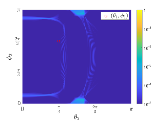
(a) NF $\rho_{{}_{\mathsf{N}}}$.

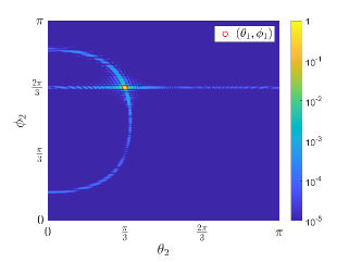
(b) FF $\rho_{{}_{\mathsf{F}}}$.

Figure 3: Illustration of the CCF with respect to $(\theta_{2},\phi_{2})$, with $M_{x}=M_{z}=65$.

$$\mathsf{C}_{\mathsf{MC}}^{\mathsf{F}}\simeq\begin{cases}\log_{2}\left(\frac{MPA}{4\pi}\min_{k=1,2}\frac{\Psi_{k}}{r_{k}^{2}\sigma_{k}^{2}}\right)\triangleq\mathsf{F}_{\mathsf{MC}}^{\mathsf{s}}&\left(\theta_{1},\phi_{1}\right)=\left(\theta_{2},\phi_{2}\right)\\ \log_{2}\left(\frac{MPA}{4\pi\left(\Psi_{1}^{-1}r_{1}^{2}\sigma_{1}^{2}+\Psi_{2}^{-1}r_{2}^{2}\sigma_{2}^{2}\right)}\right)\triangleq\mathsf{F}_{\mathsf{MC}}^{\mathsf{d}}&\left(\theta_{1},\phi_{1}\right)\neq\left(\theta_{2},\phi_{2}\right)\\ \end{cases}.$$ (61)

V-B Comparison with the FF Capacity

We next calculate the FF MC capacity.

Corollary 13.

Under the FF model, the asymptotic multicast capacity for $M\rightarrow\infty$ is given in (61), shown at the bottom of this page, which yields $\mathsf{C}_{\mathsf{MC}}^{\mathsf{F}}\simeq\mathcal{O}(\log M)$.

Proof:

Similar to the proof of Corollary 4. ∎

Remark 17.

Rather than converging to a finite value as under the NF model, the multicast capacity under the FF model can grow unboundedly with the number of the array elements, which potentially violates the energy-conservation laws.

By calculating $\mathsf{F}_{\mathsf{MC}}^{\mathsf{s}}-\mathsf{F}_{\mathsf{MC}}^{\mathsf{d}}$, we have

$$\mathsf{F}_{\mathsf{MC}}^{\mathsf{s}}-\mathsf{F}_{\mathsf{MC}}^{\mathsf{d}}=\log_{2}\left(1+\Gamma\right)\in(0,1],$$ (62)

where $\Gamma=\frac{\min_{k=1,2}r_{k}^{2}\sigma_{k}^{2}}{\max_{k=1,2}r_{k}^{2}\sigma_{k}^{2}}\in(0,1]$.

Remark 18.

The results in (62) suggest that, within the FF context, the multicast capacity is higher when the UTs are oriented in the same direction compared to when they are in different directions. This discrepancy converges to a constant not greater than one as $M$ increases.

This particular observation stems from the absence of the IUI under the MC, given that all UTs are intended to receive the same message. In this case, a high level of channel correlation is actually beneficial. Therefore, it can be concluded that unlike in the MAC and BC, the effect of NFC, i.e., the added range dimension, is not favorable for co-directional UTs in the multicast setting.

V-C Extension to Cases of $K>2$

The multicast capacity under the scenario of $K>2$ is still an open problem. However, we can derive an upper bound for multicast capacity as follows.

Proposition 2.

The multicast capacity is upper bounded as

$$\mathsf{C}_{\mathsf{MC}}\leq\log_{2}\left(1+\frac{P}{K}\sum\nolimits_{k=1}^{K}{\sigma_{k}^{-2}}\left\|\mathbf{h}_{k}\right\|^{2}\right).$$ (63)

Proof:

Please refer to Appendix -G. ∎

Given that the upper bound is articulated as a function of the channel gains, closed-form expressions for this bound can be derived for both NF and FF models. Further, we can find that when $M_{x},M_{z}\rightarrow\infty$, the NF multicast capacity has a finite upper bound $\log_{2}(1+\frac{\xi}{2K}\sum_{k=1}^{K}{\sigma_{k}^{-2}})$, while the upper bound for the FF capacity tends toward infinity.

VI Numerical Results

In this section, numerical results for the capacities of the three channels are presented. Without otherwise specification, the simulation parameter settings are defined as follows: the frequency is set as $2.4$ GHz, $d=\frac{\lambda}{2}$ m, $A=\frac{\lambda^{2}}{4\pi}$, $\frac{P_{1}}{\sigma^{2}}=\frac{P_{2}}{\sigma^{2}}=30$ dB, $\frac{P}{\sigma_{1}^{2}}=\frac{P}{\sigma_{2}^{2}}=30$ dB, $r_{1}=10$ m, and $r_{2}=5$ m. UT 1 is located in the direction $(\theta_{1},\phi_{1})=(\frac{\pi}{3},\frac{2\pi}{3})$.

VI-A CCF

Fig. 3 illustrates the values of the CCF $\rho$ when UT 2 is in various directions for both NF and FF scenarios. It can be observed that, with an array size of $65\times 65$, the CCF $\rho_{{}_{\mathsf{N}}}$ in the NF model is very close to zero regardless of UT 2’s direction, verifying that $\lim_{M_{x},{M}_{z}\rightarrow\infty}\rho_{{}_{\mathsf{N}}}\approx 0$, which demonstrates the asymptotic orthogonality of NFC for UTs in different locations. In the FF context, the value of the CCF $\rho_{{}_{\mathsf{F}}}$ is also approximately zero when UT 2 is in a distinct direction from UT 1. However, when they are located in the same direction, their channels are fully correlated, which yields $\rho_{{}_{\mathsf{F}}}=1$.

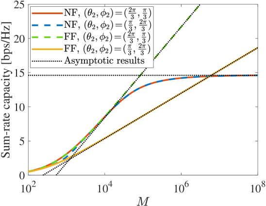
Figure 4: MAC sum-rate capacity versus $M$.

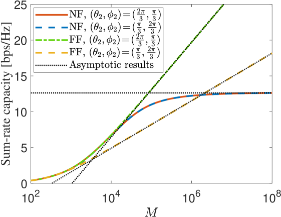
Figure 5: BC sum-rate capacity versus $M$.

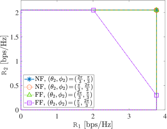
Figure 6: MAC capacity regions with $M_{x}=M_{z}=65$.

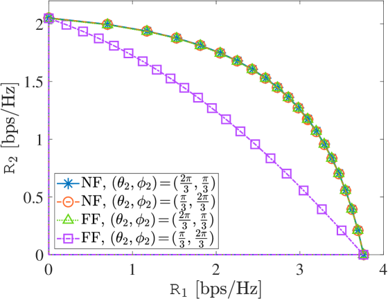
Figure 7: BC capacity regions with $M_{x}=M_{z}=65$.

VI-B MAC & BC

VI-B1 Sum-rate capacity

Fig. 5 and Fig. 5 show the sum-rate capacity of the MAC and the BC concerning the number of array elements, respectively. We can observe that under both the MAC and BC, as $M$ increases, the NF capacity and the FF capacity follow distinctly different scaling patterns. Specifically, for relatively small values of $M$, when UT 2 is in the different direction with UT 1, i.e., $(\theta_{2},\phi_{2})=(\frac{2\pi}{3},\frac{\pi}{3})$, the sum-rate capacity under the NF and FF models are similar and exhibit a linear increase with $\log M$. This similarity is attributed to the small array size, where the differences between NF and FF propagation effects are minimal and both models are accurate. However, when $M$ is sufficiently large, the disparity in channel powers and phases across the array becomes significant. In this case, the capacity under the FF model are overestimated due to the ignorance of such variations in wave propagation. As a result, the FF capacity will grow unboundedly with $M$, potentially breaking the energy-conservation laws, which is aligned with the statements in Remark 6 and 12. Conversely, as $M$ increases, the NF sum-rate capacity approach finite upper limits accurately tracked by our derived asymptotic results. This behavior is consistent with Remark 3 and 10, revealing the superior accuracy for the NF channel model.

Additionally, when UT 2 is in the same direction with UT 1, i.e., $(\theta_{2},\phi_{2})=(\frac{\pi}{3},\frac{2\pi}{3})$, for both the MAC and BC, the capacity under the FF model are lower than in the case where the UTs are in the different directions, exhibiting a smaller scaling law with $M$. These observations corroborate Remark 7 and 13. By contrast, in the NF model, the capacity for UTs in the same direction are nearly equivalent to those when they are located in different directions, surpassing the FF counterparts.

VI-B2 Capacity region

In Fig. 7 and Fig. 7, the capacity regions for the MAC and the BC are presented, respectively. It is worth to nota that the capacity regions under the NF model remain almost unchanged regardless of UT 2’s direction relative to UT 1. These regions are characterized by rectangular shapes and resemble the FF capacity regions achieved when the UTs are in the different directions. On the other hand, the FF capacity regions for the UTs located in the same direction are shaped as pentagons, diverging from the rectangular regions observed under the NF model and the FF model with UTs in different directions. In particular, the rectangular capacity regions of the NF model envelop the pentagonal regions observed in the FF model for co-directional UTs. This encapsulation underscores the superior performance of NFC in managing signal correlation and interference, offering higher channel capacity for co-directional UTs.

Moreover, Fig. 9 and Fig. 9 provide insightful visualizations of how the capacity regions for the MAC and BC evolve with changes in the number of array elements, contrasting the behaviors of NF and FF models. The visualizations demonstrate that the capacity regions under the NF model stabilize to finite areas as the array size increases, verifying the correctness of Remark 5 and 11. In contrast, the capacity regions in the FF context can expand without limitation with the number of array elements, which is unreasonable under energy consideration and justifies the statements in Remark 8 and 14.

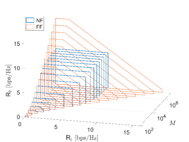
(a) $(\theta_{2},\phi_{2})=(\frac{\pi}{3},\frac{2\pi}{3})$.

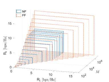
(b) $(\theta_{2},\phi_{2})=(\frac{2\pi}{3},\frac{\pi}{3})$.

Figure 8: MAC capacity region versus $M$.

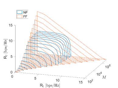
(a) $(\theta_{2},\phi_{2})=(\frac{\pi}{3},\frac{2\pi}{3})$.

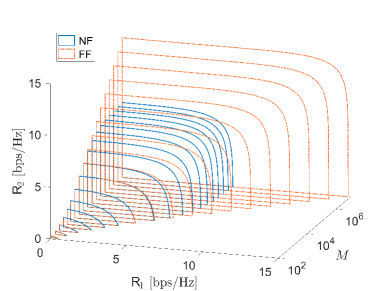
(b) $(\theta_{2},\phi_{2})=(\frac{2\pi}{3},\frac{\pi}{3})$.

Figure 9: BC capacity region versus $M$.

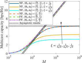
(a) Multicast Capacity versus $M$ with different $\xi$.

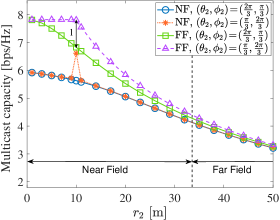
(b) Multicast Capacity versus $r_{2}$ with $M_{x}\!=\!M_{z}\!=\!551$.

Figure 10: Multicast capacity.

VI-C MC

Fig. 9 demonstrates the multicast capacity versus $M$, with different values of the AOR $\xi$. For the NF case, the musticast capacity converge to finite upper limits accurately tracked by our derived asymptotic results, which are positively correlated to the values of $\xi$. This behavior validates the conclusions in Remark 16. Additionally, contrary to the patterns observed in the MAC and BC, the FF multicast capacity for co-directional UTs exceeds that for UTs in different directions by a small gap which tend to be constant as $M$ becomes large. This distinct observation verifies Remark 18 and is attributed to the unique nature of the MC, where transmitting the same message to all UTs benefits from a high level of channel correlation.

In Fig. 10(b), we present the multicast capacity as functions of the UT 2’s distance $r_{2}$ with $r_{1}=10$ fixed at $10$ m. We can observe that, for a large number of antennas, the multicast capacity under the FF model are markedly overestimated when the UTs are located near the BS, while this overestimation diminishes as the distance from the UT to the BS increase. This is because the effect of the NF is pronounced at short distances, and will be alleviated as the UT move toward the far field. Further, the two lines under NF models are almost overlapping, with a notable exception at $r_{2}=10$ m. At this point, the scenario where UT 2 is in the same location as UT 1 exhibits a markedly higher capacity, highlighting the preference for high channel correlation in multicast settings. Regarding the FF case, the gap between the two lines initially increases with $r_{2}$, reaching a peak when UTs are equidistant from the BS ($\Gamma=1$). Beyond this point, as $r_{2}$ continues to increase, the gap decreases in accordance with $\Gamma$, as demonstrated in (62).

VII Conclusion

This article has investigated the channel capacity of NF multiuser communications, by specializing the multiuser channels into the MAC, BC and MC. We derived the sum-rates capacity and capacity regions for the MAC and BC, and the multicast capacity for the MC. By comparing the results with the FF counterparts, we have drawn the following conclusions: 1) the additional asymptotic orthogonality of NFC in the distance domain can improve capacity of the MAC and BC for co-directional users, but it is not beneficial to the MC; 2) rather than growing unboundedly, the NF capacity of the three channels converge to finite values as the number of array elements increases, underscoring the importance of accurate channel modeling for NFC.

-A Proof of Lemma 1

By defining ${\mathbf{H}}\triangleq[\sqrt{P_{1}}{\mathbf{h}}_{1}\sqrt{P_{2}}{\mathbf{h}}_{2}]\in{\mathbbmss{C}}^{M\times 2}$, (10) can be rewritten as

$${\mathsf{C}}_{\mathsf{MAC}}=\log_{2}\det\left({\mathbf{I}}+\sigma^{-2}{\mathbf{H}}{\mathbf{H}}^{\mathsf{H}}\right).$$ (A1)

Based on the Sylvester’s theorem, (A1) can be calculated as follows:

$${\mathsf{C}}_{\mathsf{MAC}}=\log_{2}\det\left({\mathbf{I}}+\sigma^{-2}{\mathbf{H}}^{\mathsf{H}}{\mathbf{H}}\right)$$ (A2)

$$=\log_{2}\det\!\left[\begin{matrix}1\!+\!P_{1}\sigma^{-2}\lVert{\mathbf{h}}_{1}\rVert^{2}&\!1\!+\!\sqrt{P_{1}P_{2}}\sigma^{-2}{\mathbf{h}}_{1}^{\mathsf{H}}{\mathbf{h}}_{2}\\ 1\!+\!\sqrt{P_{1}P_{2}}\sigma^{-2}{\mathbf{h}}_{2}^{\mathsf{H}}{\mathbf{h}}_{1}&\!1\!+\!P_{2}\sigma^{-2}\lVert{\mathbf{h}}_{2}\rVert^{2}\\ \end{matrix}\right].$$

The results of (11) can be then obtained by calculating the above determinant of the $2\times 2$ matrix and performing simple manipulations.

-B Proof of Theorem 1

Based on (1) and (5), $\left\|\mathbf{h}_{k}\right\|^{2}$ under the NF model can be calculated as

$$\begin{split}&G_{k}=\frac{A\Psi_{k}}{4\pi r_{k}^{2}}\sum\nolimits_{m_{x}\in\mathcal{M}_{x}}\sum\nolimits_{m_{z}\in\mathcal{M}_{z}}\\ &~{}~{}\times\big{(}(m_{x}^{2}+m_{z}^{2})\epsilon_{k}^{2}-2m_{x}\epsilon_{k}\Phi_{k}-2m_{z}\epsilon_{k}\Omega_{k}+1\big{)}^{-\frac{3}{2}}.\end{split}$$ (A3)

We define the function

$$f\left(x,z\right)\triangleq(x^{2}+z^{2}-2\Phi_{k}x-2\Omega_{k}z+1)^{-\frac{3}{2}}$$ (A4)

in the rectangular area $\mathcal{H}=\left\{\left(x,z\right)\mid-\frac{M_{x}\epsilon_{k}}{2}\leq x\leq\frac{M_{x}\epsilon_{k}}{2},-\frac{M_{z}\epsilon_{k}}{2}\leq z\leq\frac{M_{z}\epsilon_{k}}{2}\right\}$ that is then partitioned into $M_{x}M_{z}$ sub-rectangles, each with equal area $\epsilon_{k}^{2}$. Since $\epsilon_{k}\ll 1$, we have $f\left(x,z\right)\approx f\left(m_{x}\epsilon_{k},m_{z}\epsilon_{k}\right)$ for $\forall\left(x,z\right)\in\left\{\left(x,z\right)\mid\left(m_{x}-\frac{1}{2}\right)\epsilon_{k}\leq x\leq\left(M_{x}+\frac{1}{2}\right)\epsilon_{k},\left(m_{z}-\frac{1}{2}\right)\epsilon_{k}\leq z\right.$ $\left.\leq\left(m_{z}+\frac{1}{2}\right)\epsilon_{k}\right\}$. Based on the concept of integral, we have

$$\sum\nolimits_{m_{x},m_{z}}{f\left(m_{x}\epsilon_{k},m_{z}\epsilon_{k}\right)\epsilon_{k}^{2}}\approx\iint_{\mathcal{H}}{f\left(x,z\right)dxdz}.$$ (A5)

As a result, (A3) can be rewritten as

$$\begin{split}G_{k}&=\frac{\xi\Psi_{k}}{4\pi}\int_{-\frac{M_{z}\epsilon_{k}}{2}}^{\frac{M_{z}\epsilon_{k}}{2}}{\int_{-\frac{M_{x}\epsilon_{k}}{2}}^{\frac{M_{x}\epsilon_{k}}{2}}}\\ &~{}~{}\times(x^{2}+z^{2}-2\Phi_{k}x-2\Omega_{k}z+1)^{-\frac{3}{2}}dxdz.\end{split}$$ (A6)

We can calculate the inner integral with the aid of [25, Eq. (2.264.5)] and then the outer integral with the aid of [25, Eq. (2.284.5)], which yields the results of (14). After obtaining the channel gains, the expressions of $\rho_{{}_{\mathsf{N}}}$ in (15) can be derived by the definition of the CCF with some mathematical manipulations.

-C Proof of Corollary 2

With $M_{x}=1$ and $M_{z}=M$, (14) can be rewritten as

$$G_{k}=\frac{\xi}{4\pi}\sum\nolimits_{x\in\mathcal{X}^{\prime}_{k}}{\sum\nolimits_{z\in\mathcal{Z}^{\prime}_{k}}{\delta_{k}\left(x,z\right)}}\triangleq g(\epsilon_{k}),$$ (A7)

where $\mathcal{X}^{\prime}_{k}=\left\{\frac{\epsilon_{k}}{2}\pm\Phi_{k}\right\}$, and $\mathcal{Z}^{\prime}_{k}=\left\{\frac{M\epsilon_{k}}{2}\pm\Omega_{k}\right\}$. Since $\epsilon_{k}\ll 1$, we can utilizing the first-order Taylor approximation $G_{k}\approx f\left(0\right)+f^{\prime}\left(0\right)\epsilon_{k}$, leading to the results of (19). When $M\rightarrow\infty$, we can obtain $\lim_{M\rightarrow\infty}G_{k}=\frac{\xi\epsilon_{k}\sin\phi_{k}}{2\pi\sin\theta_{k}}$ by applying L’Hôpital’s rule, which yield the results of (2).

-D Proof of Lemma 2

When the SIC decoding order $1\rightarrow 2$ is employed, the message of UT 1 is decoded firstly by treating the message of UT 2 as interference. In this case, the rate of UT 1 reads

$${\mathsf{R}}_{1}^{1\rightarrow 2}=\log_{2}\det({\mathbf{I}}+{P_{1}}{\sigma^{-2}}{\mathbf{h}}_{1}{\mathbf{h}}_{1}^{\mathsf{H}}({\mathbf{I}}+{P_{2}}{\sigma^{-2}}{\mathbf{h}}_{2}{\mathbf{h}}_{2}^{\mathsf{H}})^{-1})$$

$$\overset{(a)}{=}\!\log_{2}\left(1+{P_{1}}{\sigma^{-2}}\mathbf{h}_{1}^{\mathsf{H}}\left(\mathbf{I}+{P_{2}}{\sigma^{-2}}\mathbf{h}_{2}\mathbf{h}_{2}^{\mathsf{H}}\right)^{-1}\mathbf{h}_{1}\right)$$ (A8)

$$\overset{(b)}{=}\log_{2}\!\left(\!1\!+\!{P_{1}}{\sigma^{-2}}\mathbf{h}_{1}^{\mathsf{H}}\bigg{(}\mathbf{I}\!-\!\frac{{P_{2}}{\sigma^{-2}}\mathbf{h}_{2}\mathbf{h}_{2}^{\mathsf{H}}}{1\!+\!{P_{2}}{\sigma^{-2}}\left\|\mathbf{h}_{2}\right\|^{2}}\bigg{)}\mathbf{h}_{1}\right),$$ (A9)

where equality $(a)$ is attained by using the Sylvester’s theorem, and $(b)$ is attained by using the Woodbury matrix identity. The results of (22a) can be obtained by performing some manipulations on (A9). After the message of UT 1 is decoded, it will be removed from the received signal, and the message of UT 2 will be decoded without interference. Consequently, the rate of UT 2 is given by

$${\mathsf{R}}_{2}^{1\rightarrow 2} =\log_{2}\det(\mathbf{I}+\mathbf{h}_{2}\mathbf{h}_{2}^{\mathsf{H}})\overset{\left(a\right)}{=}\log_{2}\!\left(1+P_{2}\sigma^{-2}G_{2}\right),$$

where $(a)$ follows from the Sylvester’s theorem. ${\mathsf{R}}_{1}^{2\rightarrow 1}$ and ${\mathsf{R}}_{2}^{2\rightarrow 1}$ can be derived following the similar steps.

-E Proof of Proposition 1

The channel gains are easily derived from (6). On this basis, the CCF can be written as follows:

$$\!\rho_{{}_{\mathsf{F}}}\!=\frac{1}{M^{2}}\left|\sum\nolimits_{m_{x}\in\mathcal{M}_{x}}{\sum\nolimits_{m_{z}\in\mathcal{M}_{z}}{\mathrm{e}^{\mathrm{j}\left(m_{x}\Delta_{\Phi}+m_{z}\Delta_{\Omega}\right)}}}\right|^{2}.$$ (A10)

When $\Phi_{1}\neq\Phi_{2}$ and $\Omega_{1}\neq\Omega_{2}$, $\rho_{{}_{\mathsf{F}}}$ can be derived as follows:

$$\rho_{{}_{\mathsf{F}}}\! \overset{\left(a\right)}{=}\!\frac{1}{M^{2}}\!\left|\!\frac{\big{(}\mathrm{e}^{\mathrm{j}\left(\tilde{M}_{x}\!+\!1\right)\Delta_{\Phi}}\!-\!\mathrm{e}^{-\mathrm{j}\tilde{M}_{x}\Delta_{\Phi}}\big{)}\!\big{(}\mathrm{e}^{\mathrm{j}\left(\tilde{M}_{z}\!+\!1\right)\Delta_{\Omega}}\!-\!\mathrm{e}^{-\mathrm{j}\tilde{M}_{z}\Delta_{\Omega}}\big{)}}{\left(\mathrm{e}^{\mathrm{j}\Delta_{\Phi}}-1\right)\left(\mathrm{e}^{\mathrm{j}\Delta_{\Omega}}-1\right)}\!\right|^{2}$$

$$\overset{\left(b\right)}{=}\frac{16\sin^{2}\left(\frac{M_{x}\Delta_{\Phi}}{2}\right)\sin^{2}\left(\frac{M_{z}\Delta_{\Omega}}{2}\right)}{M^{2}\left(1-\cos\Delta_{\Omega}\right)^{2}\left(1-\cos\Delta_{\Phi}\right)^{2}}$$

$$~{}~{}~{}\times\left|\sin\frac{\Delta_{\Phi}}{2}\sin\frac{\Delta_{\Omega}}{2}-\mathrm{j}\sin\frac{\Delta_{\Phi}}{2}\sin\frac{\Delta_{\Omega}}{2}\right|^{2},$$ (A11)

where $(a)$ follows from the sum of the geometric series, and $(b)$ holds due to Euler’s formula and trigonometric identities. The final results can be obtained by calculating the magnitude. For the cases $\left(\theta_{1},\phi_{1}\right)=\left(\theta_{2},\phi_{2}\right)$, $\Phi_{1}\neq\Phi_{2},\Omega_{1}=\Omega_{2}$ and $\Phi_{1}=\Phi_{2},\Omega_{1}\neq\Omega_{2}$, (A10) can be simplified as $1$, $\frac{1}{M^{2}}\left|\sum_{m_{x}=-\tilde{M}_{x}}^{\tilde{M}_{x}}{\mathrm{e}^{\mathrm{j}m_{x}\Delta_{\Phi}}}\right|^{2}$ and $\frac{1}{M^{2}}\left|\sum_{m_{z}=-\tilde{M}_{z}}^{\tilde{M}_{z}}{\mathrm{e}^{\mathrm{j}m_{z}\Delta_{\Omega}}}\right|^{2}$, respectively, which can be calculated with similar steps to (-E).

-F Proof of Theorem 3

The optimal solution of problem (55) can be derived from the KKT conditions as follows:

$$\nabla(-t)+\eta\nabla(\lVert{\mathbf{w}}\rVert^{2}-1)+\mu_{1}\nabla(t-\lvert{\bar{\mathbf{h}}}_{1}^{\mathsf{H}}\mathbf{w}\rvert^{2})$$

$$\qquad\qquad\qquad\qquad\qquad\ +\mu_{2}\nabla(t-\lvert{\bar{\mathbf{h}}}_{2}^{\mathsf{H}}\mathbf{w}\rvert^{2})={\mathbf{0}},$$ (A12)

$$\mu_{1}(t-\lvert{\bar{\mathbf{h}}}_{1}^{\mathsf{H}}\mathbf{w}\rvert^{2})=0,\ \mu_{2}(t-\lvert{\bar{\mathbf{h}}}_{2}^{\mathsf{H}}\mathbf{w}\rvert^{2})=0,$$ (A13)

$$\mu_{1}\geq 0,\ \mu_{2}\geq 0,\ \eta\in{\mathbbmss{R}},$$ (A14)

where $\bar{\mathbf{h}}_{1}=\sigma_{1}^{-1}\mathbf{h}_{1}$, $\bar{\mathbf{h}}_{2}=\sigma_{2}^{-1}\mathbf{h}_{2}$, and $\{\eta,\mu_{1},\mu_{2}\}$ are real-valued Lagrangian multipliers. From (A12), we can obtain

$$\mu_{1}+\mu_{2}=1,$$ (A15)

$$(\mu_{1}{\bar{\mathbf{h}}}_{1}{\bar{\mathbf{h}}}_{1}^{\mathsf{H}}+\mu_{2}{\bar{\mathbf{h}}}_{2}{\bar{\mathbf{h}}}_{2}^{\mathsf{H}}){\mathbf{w}}=\eta{\mathbf{w}}.$$ (A16)

It follows from (A15) that $\mu_{1}$ and $\mu_{2}$ cannot be $0$ at the same time. Particularly, three different cases are discussed as follows.

-F1 $\mu_{1}=1$ and $\mu_{2}=0$

: In this case, we have $t=\lvert{\bar{\mathbf{h}}}_{1}^{\mathsf{H}}\mathbf{w}\rvert^{2}$, from which we can readily deduce the optimal solutions ${\mathbf{w}^{\star}}={{\mathbf{h}}_{1}}/{\lVert{\mathbf{h}}_{1}\rVert}$ and $t^{\star}=\lVert{\bar{\mathbf{h}}}_{1}\rVert^{2}$. Substituting the results into the constraint (55b) yields ${\lVert{\bar{\mathbf{h}}}_{1}\rVert^{2}\leq\rho\lVert{\bar{\mathbf{h}}}_{2}\rVert^{2}}$.

-F2 $\mu_{1}=0$ and $\mu_{2}=1$

: Following similar steps to the first case, we can obtain ${\mathbf{w}^{\star}}={{\mathbf{h}}_{2}}/{\lVert{\mathbf{h}}_{2}\rVert}$ with the condition ${\lVert{\bar{\mathbf{h}}}_{2}\rVert^{2}\leq\rho\lVert{\bar{\mathbf{h}}}_{1}\rVert^{2}}$.

-F3 $\mu_{1}>0$ and $\mu_{2}>0$

: In this case, we have

$$t=\lvert{\bar{\mathbf{h}}}_{1}^{\mathsf{H}}\mathbf{w}\rvert^{2}=\lvert{\bar{\mathbf{h}}}_{2}^{\mathsf{H}}\mathbf{w}\rvert^{2}.$$ (A17)

According to (A16) and (A17), we can write $\mathbf{w}$ as a linear combination of ${\bar{\mathbf{h}}}_{1}$ and ${\bar{\mathbf{h}}}_{2}$:

$${\mathbf{w}}=a{\bar{\mathbf{h}}}_{1}+b{\bar{\mathbf{h}}}_{2}$$ (A18)

with $\frac{a}{b}=\frac{{\mu_{1}}}{{\mu_{2}}{\rm{e}}^{-{\rm{j}}\angle({\mathbf{h}}_{1}^{\mathsf{H}}{\mathbf{h}}_{2})}}$. Substituting (A18) into (A16) gives

$${\mu_{1}}\Big{(}\lVert{\bar{\mathbf{h}}}_{1}\rVert^{2}+\frac{b}{a}{\bar{\mathbf{h}}}_{1}^{\mathsf{H}}{\bar{\mathbf{h}}}_{2}\Big{)}={\mu_{2}}\Big{(}\lVert{\bar{\mathbf{h}}}_{2}\rVert^{2}+\frac{a}{b}{\bar{\mathbf{h}}}_{2}^{\mathsf{H}}{\bar{\mathbf{h}}}_{1}\Big{)}=\eta.$$ (A19)

By combining (A19) and (A15), we can derive $\mu_{1}=\frac{\left\|\bar{\mathbf{h}}_{2}\right\|^{2}-\left|\bar{\mathbf{h}}_{1}^{\mathsf{H}}\bar{\mathbf{h}}_{2}\right|}{\left\|\bar{\mathbf{h}}_{1}\right\|^{2}+\left\|\bar{\mathbf{h}}_{2}\right\|^{2}-2\left|\bar{\mathbf{h}}_{1}^{\mathsf{H}}\bar{\mathbf{h}}_{2}\right|}$, $\mu_{2}=\frac{\left\|\bar{\mathbf{h}}_{1}\right\|^{2}-\left|\bar{\mathbf{h}}_{1}^{\mathsf{H}}\bar{\mathbf{h}}_{2}\right|}{\left\|\bar{\mathbf{h}}_{1}\right\|^{2}+\left\|\bar{\mathbf{h}}_{2}\right\|^{2}-2\left|\bar{\mathbf{h}}_{1}^{\mathsf{H}}\bar{\mathbf{h}}_{2}\right|}$, and $\eta=\frac{\left\|\bar{\mathbf{h}}_{1}\right\|^{2}\left\|\bar{\mathbf{h}}_{2}\right\|^{2}-\left|\bar{\mathbf{h}}_{1}^{\mathsf{H}}\bar{\mathbf{h}}_{2}\right|^{2}}{\left\|\bar{\mathbf{h}}_{1}\right\|^{2}+\left\|\bar{\mathbf{h}}_{2}\right\|^{2}-2\left|\bar{\mathbf{h}}_{1}^{\mathsf{H}}\bar{\mathbf{h}}_{2}\right|}$. Given the prerequisites $\mu_{1}>0$ and $\mu_{2}>0$, it is required that ${\lVert{\bar{\mathbf{h}}}_{1}\rVert^{2}\geq\rho\lVert{\bar{\mathbf{h}}}_{2}\rVert^{2}}$ and ${\lVert{\bar{\mathbf{h}}}_{2}\rVert^{2}\geq\rho\lVert{\bar{\mathbf{h}}}_{1}\rVert^{2}}$ in this case. Consequently, since $\lVert{\mathbf{w}}\rVert=1$, $\mathbf{w}$ can be expressed as

$${\mathbf{w}}=\frac{\mu_{1}{\bar{\mathbf{h}}}_{1}+\mu_{2}{\bar{\mathbf{h}}}_{2}{\rm{e}}^{-{\rm{j}}\angle({\mathbf{h}}_{1}^{\mathsf{H}}{\mathbf{h}}_{2})}}{\sqrt{\mu_{1}^{2}\lVert{\bar{\mathbf{h}}}_{1}\rVert^{2}+\mu_{2}^{2}\lVert{\bar{\mathbf{h}}}_{2}\rVert^{2}+2\mu_{1}\mu_{2}\lvert{\bar{\mathbf{h}}}_{1}^{\mathsf{H}}{\bar{\mathbf{h}}}_{2}\rvert}}.$$ (A20)

It is worth noting that $\eta=\mu_{1}^{2}\lVert{\bar{\mathbf{h}}}_{1}\rVert^{2}+\mu_{2}^{2}\lVert{\bar{\mathbf{h}}}_{2}\rVert^{2}+2\mu_{1}\mu_{2}\lvert{\bar{\mathbf{h}}}_{1}^{\mathsf{H}}{\bar{\mathbf{h}}}_{2}\rvert$. Finally, the optimal beamforming vector under the case of $\mu_{1}>0$ and $\mu_{2}>0$ is obtained as

$$\mathbf{w}^{\star}=\frac{\mu_{1}}{\sqrt{\eta}\sigma_{1}}\mathbf{h}_{1}+\frac{\mu_{2}}{\sqrt{\eta}\sigma_{2}}\mathbf{h}_{2}{\rm{e}}^{-{\rm{j}}\angle({\mathbf{h}}_{1}^{\mathsf{H}}{\mathbf{h}}_{2})}.$$ (A21)

Taking the three cases together with the substitutions of $\lVert{\mathbf{h}}_{k}\rVert^{2}=G_{k}$ and $\rho=\rho_{{}_{\mathsf{N}}}$, we can obtain the results in (56), which then lead to the multicast capacity in (57).

-G Proof of Proposition 2

Based on (53), the MC capacity satisfies

$$\mathsf{C}_{\mathsf{MC}} \leq\max_{\mathbf{\Sigma}\succeq 0,\mathsf{tr}(\mathbf{\Sigma})\leq P}\log_{2}\left(1+\frac{1}{K}\sum\nolimits_{k=1}^{K}{\frac{\mathbf{h}_{k}^{\mathsf{H}}\mathbf{\Sigma h}_{k}}{\sigma_{k}^{2}}}\right),$$

$$=\max_{\mathbf{\Sigma}\succeq 0,\mathsf{tr}(\mathbf{\Sigma})\leq P}\log_{2}\left(1+\frac{1}{K}\mathrm{tr}\left(\mathbf{\Sigma}\sum\nolimits_{k=1}^{K}{\frac{\mathbf{h}_{k}\mathbf{h}_{k}^{\mathsf{H}}}{\sigma_{k}^{2}}}\right)\right)$$

$$\leq\max_{\mathbf{\Sigma}\succeq 0,\mathsf{tr}(\mathbf{\Sigma})\leq P}\log_{2}\left(1+\frac{1}{K}\mathrm{tr}\left(\mathbf{\Sigma}\right)\mathrm{tr}\left(\sum\nolimits_{k=1}^{K}{\frac{\mathbf{h}_{k}\mathbf{h}_{k}^{\mathsf{H}}}{\sigma_{k}^{2}}}\right)\right)$$

$$=\log_{2}\left(1+\frac{P}{K}\sum\nolimits_{k=1}^{K}{\sigma_{k}^{-2}\left\|\mathbf{h}_{k}\right\|^{2}}\right).$$ (A22)

References

- [1] Y. Liu et al., “Near-field communications: A tutorial review,” IEEE Open J. Commun. Soc., vol. 4, pp. 1999–2049, 2023.
- [2] H. Zhang et al., “6G wireless communications: From far-field beam steering to near-field beam focusing,” IEEE Commun. Mag., vol. 61, no. 4, pp. 72–77, Apr. 2023.
- [3] ——, “Beam focusing for near-field multiuser MIMO communications,” IEEE Trans. Wireless Commun., vol. 21, no. 9, pp. 7476–7490, Sep. 2022.
- [4] Z. Wang, X. Mu, and Y. Liu, “TTD configurations for near-field beamforming: Parallel, serial, or hybrid?” IEEE Trans. Commun., Early Access, 2024.
- [5] Y. Liu et al., “Near-field communications: A comprehensive survey,” arXiv preprint arXiv:2401.05900, 2024.
- [6] H. Lu and Y. Zeng, “Near-field modeling and performance analysis for multi-user extremely large-scale MIMO communication,” IEEE Commun. Lett., vol. 26, no. 2, pp. 277–281, Feb 2022.
- [7] A. Goldsmith, S. Jafar, N. Jindal, and S. Vishwanath, “Capacity limits of MIMO channels,” IEEE J. Sel. Areas Commun., vol. 21, no. 5, pp. 684–702, Jun. 2003.
- [8] A. El Gamal and T. M. Cover, “Multiple user information theory,” Proc. IEEE, vol. 68, no. 12, pp. 1466–1483, Dec. 1980.
- [9] A. El Gamal and Y.-H. Kim, Network Information Theory. New York, NY, USA: Cambridge Univ. Press, 2011.
- [10] W. Yu, W. Rhee, S. Boyd, and J. M. Cioffi, “Iterative water-filling for Gaussian vector multiple-access channels,” IEEE Trans. Inf. Theory, vol. 50, no. 1, pp. 145–152, Jan. 2004.
- [11] H. Weingarten, Y. Steinberg, and S. S. Shamai, “The capacity region of the Gaussian multiple-input multiple-output broadcast channel,” IEEE Trans. Inf. Theory, vol. 52, no. 9, pp. 3936–3964, Sep. 2006.
- [12] N. Jindal and Z.-Q. Luo, “Capacity limits of multiple antenna multicast,” in IEEE Int. Symp. Inf. Theory. IEEE, 2006, pp. 1841–1845.
- [13] L. Cui, S.-G. Zhou, J.-Y. Li, L.-W. Zhu, and S. Li, “The near-field capacity analysis for large antenna array,” in Proc. IEEE 95th Veh. Technol. Conf. (VTC-Spring), Jun. 2022, pp. 1–5.
- [14] Z. Xie, Y. Liu, J. Xu, X. Wu, and A. Nallanathan, “Performance analysis for near-field MIMO: Discrete and continuous aperture antennas,” IEEE Wireless Commun. Lett., vol. 12, no. 12, pp. 2258–2262, Dec. 2023.
- [15] S. Guo and K. Qu, “Beamspace modulation for near field capacity improvement in XL-MIMO communications,” IEEE Wireless Commun. Lett., vol. 12, no. 8, pp. 1434–1438, Aug. 2023.
- [16] Z. Wu, M. Cui, Z. Zhang, and L. Dai, “Distance-aware precoding for near-field capacity improvement in XL-MIMO,” in Proc. IEEE 95th Veh. Technol. Conf. (VTC-Spring), Jun. 2022, pp. 1–5.
- [17] T. Gong et al., “Holographic MIMO communications with arbitrary surface placements: Near-field los channel model and capacity limit,” IEEE J. Sel. Areas Commun., Early Access, 2024.
- [18] C. Ouyang et al., “On the impact of reactive region on the near-field channel gain,” arXiv preprint arXiv:2404.08343, 2024.
- [19] B. Zhao, C. Ouyang, Y. Liu, X. Zhang, and H. V. Poor, “Modeling and analysis of near-field ISAC,” IEEE J. Sel. Top. Sign. Proces., pp. 1–16, Early Access, 2024.
- [20] B. Suard, G. Xu, H. Liu, and T. Kailath, “Uplink channel capacity of space-division-multiple-access schemes,” IEEE Trans. Inf. Theory, vol. 44, no. 4, pp. 1468–1476, Jul. 1998.
- [21] M. Costa, “Writing on dirty paper,” IEEE Trans. Inf. Theory, vol. 29, no. 3, pp. 439–441, May 1983.
- [22] S. Vishwanath, N. Jindal, and A. Goldsmith, “Duality, achievable rates, and sum-rate capacity of Gaussian MIMO broadcast channels,” IEEE Trans. Inf. Theory, vol. 49, no. 10, pp. 2658–2668, Oct. 2003.
- [23] N. Jindal, W. Rhee, S. Vishwanath, S. Jafar, and A. Goldsmith, “Sum power iterative water-filling for multi-antenna Gaussian broadcast channels,” IEEE Trans. Inf. Theory, vol. 51, no. 4, pp. 1570–1580, Apr. 2005.
- [24] S. Y. Park and D. J. Love, “Capacity limits of multiple antenna multicasting using antenna subset selection,” IEEE Trans. Signal Process., vol. 56, no. 6, pp. 2524–2534, Jun. 2008.
- [25] I. S. Gradshteyn and I. M. Ryzhik, Table of Integrals, Series and Products, 7th ed. New York, NY, USA: Academic Press, 2007.