Certifying Euclidean Sections and Finding Planted Sparse Vectors Beyond the $\sqrt{n}$ Dimension Threshold

Abstract

We consider the task of certifying that a random $d$-dimensional subspace $X$ in $\mathbb{R}^{n}$ is well-spread — every vector $x\in X$ satisfies $c\sqrt{n}\|x\|_{2}\leqslant\|x\|_{1}\leqslant\sqrt{n}\|x\|_{2}$. In a seminal work, Barak et. al. [BBH⁺12] showed a polynomial-time certification algorithm when $d\leqslant O(\sqrt{n})$. On the other hand, when $d\gg\sqrt{n}$, the certification task is information-theoretically possible but there is evidence that it is computationally hard [MW21, Cd22], a phenomenon known as the information-computation gap.

In this paper, we give subexponential-time certification algorithms in the $d\gg\sqrt{n}$ regime. Our algorithm runs in time $\exp(\widetilde{O}(n^{\varepsilon}))$ when $d\leqslant\widetilde{O}(n^{\frac{1+\varepsilon}{2}})$, establishing a smooth trade-off between runtime and the dimension.

Our techniques naturally extend to the related planted problem, where the task is to recover a sparse vector planted in a random subspace. Our algorithm achieves the same runtime and dimension trade-off for this task.

1 Introduction

For any vector $x\in\mathbb{R}^{n}$, we know that $\|x\|_{2}\leqslant\|x\|_{1}\leqslant\sqrt{n}\|x\|_{2}$. Intuitively, if the upper bound is approximately tight, i.e., $\|x\|_{1}\geqslant c\sqrt{n}\|x\|_{2}$, then $x$ is “dense” or “incompressible”. We say that a subspace $X\subseteq\mathbb{R}^{n}$ is well-spread if every $x\in X$ is dense. More formally, we define the distortion of $X$, denoted $\Delta(X)$, as follows,

$$\Delta(X)\coloneqq\sup_{x\in X:\ x\neq 0}\frac{\sqrt{n}\|x\|_{2}}{\|x\|_{1}}\,.$$ (1)

The distortion always satisfies $1\leqslant\Delta(X)\leqslant\sqrt{n}$. Subspaces with large dimension $d$ and small distortion are called good Euclidean sections of $\ell_{1}^{n}$. In particular, they provide embeddings of $\ell_{2}^{d}$ into $\ell_{1}^{n}$ with only a small blow-up in the dimension, thus such subspaces have many applications including error-correcting codes over the reals [CT05, GLW08], compressed sensing [KT07, Don06], high-dimensional nearest-neighbor search [Ind06], and oblivious regression [dLN⁺21].

Therefore, there has been a long line of work on constructing good Euclidean sections, including explicit constructions [Ind06, Ind07, GLR10] and constructions requiring few random bits (a.k.a. partially derandomized constructions) [LS08, GLW08, IS10]. However, all such constructions suffer in either the dimension or the distortion (see [IS10] and references therein).

On the other hand, it is well known that a fully random subspace of $\mathbb{R}^{n}$ of dimension $d=\Omega(n)$ (for instance, the column space of an $n\times d$ matrix with i.i.d. Gaussian or $\pm 1$ entries) has $O(1)$ distortion with high probability [FLM77, Kas77, GG84]. However, randomized constructions suffer from the drawback that the output is not guaranteed to always satisfy the desired properties. Thus, certifying randomized constructions is often considered as a functional proxy when explicit constructions are hard to come by, as is the case for Euclidean sections.

This motivates the algorithmic task of certifying that a random subspace is well-spread. With $\exp(d)$ time, this problem is trivial as we can brute-force search over an $\varepsilon$-net in $\mathbb{R}^{d}$. The best known non-trivial result is by Barak et. al. [BBH⁺12], who showed that given a random matrix $A\in\mathbb{R}^{n\times d}$ with i.i.d. Gaussian entries and $d\lesssim\sqrt{n}$, there is a polynomial-time algorithm certifying that $\operatorname{colspan}(A)$ has $O(1)$ distortion (with high probability over $A$). However, no efficient certification algorithm is known when $d\gg\sqrt{n}$ (note that the problem is harder for larger $d$).

More recently, “evidence” of computational hardness was established for the $d\gg\sqrt{n}$ regime in the form of lower bounds against low-degree polynomials [MW21, Cd22]. This suggests that there is an information-computation gap for this problem with the computational threshold at $d\sim\sqrt{n}$, i.e., any polynomial-time algorithm for $d\gg\sqrt{n}$ would require significant breakthroughs (see e.g. [Hop18, KWB19] for expositions of the low-degree hardness framework).

The lower bounds by [MW21, Cd22] leave open the possibility of subexponential-time certification algorithms when $d$ is between $\sqrt{n}$ and $n$. This sets the stage for our first result.

Theorem 1 (Informal Theorem 3.3).

Fix $\varepsilon\in(0,1)$, and let $d,n\in\mathbb{N}$ such that $d=O(n^{\frac{1+\varepsilon}{2}}/\log n)$. Let $A\sim\mathcal{N}(0,1)^{n\times d}$. Then, there is a certification algorithm that runs in $2^{\widetilde{O}(n^{\varepsilon})}$ time and, with probability $1-o(1)$ over $A$, certifies that $\operatorname{colspan}(A)$ has $O(1)$ distortion.

Notice that 1 establishes a smooth trade-off between the dimension $d$ and the runtime. Specifically, when $\varepsilon=0$, we have $d\leqslant\widetilde{O}(\sqrt{n})$ and the runtime is polynomial, matching the best known algorithm by [BBH⁺12]. When $\varepsilon$ increases to $1$, the dimension $d$ increases to $n$ while the runtime increases to exponential.

We note that the phenomenon of information-computation gap is widespread across a variety of certification and inference problems. For these problems, there is a parameter regime (often called the “hard” regime) in which it is conjectured that no polynomial-time algorithm exists. In many cases, smooth trade-offs were established between runtime and the problem parameters, similar to that of 1. Examples of such trade-offs include runtime vs. the number of constraints in refuting random constraint satisfaction problems [RRS17, GKM22, HKM23], runtime vs. the approximation factor in polynomial optimization or tensor PCA [BGG⁺17, WAM19, HKPT24], runtime vs. the sparsity parameter in certifying the restricted isometry property (RIP) for random matrices [KZ14, DKWB21], and runtime vs. the sparsity of the hidden vector in sparse PCA [dKNS20, DKWB23].

Finding planted sparse vector in a random subspace.

For average-case optimization problems, techniques for certification can often be adapted to solving the search problem for the related planted model; this is called the proofs-to-algorithms paradigm [FKP19] in the literature. For the problem of certifying distortion of a random subspace (in which there is no sparse vector), the corresponding planted problem is to find a sparse vector planted in a random subspace.

We first formally define the planted sparse vector problem:

Model 1 (Planted sparse vector problem).

Fix an unknown unit vector $v\in\mathbb{R}^{n}$, and let $d\leqslant n\in\mathbb{N}$. Let $\widetilde{A}$ be a random $n\times d$ matrix sampled as follows: (1) let $A$ be the random matrix such that the first column is $v$ and the other $d-1$ columns are i.i.d. $\mathcal{N}(0,\frac{1}{n}\mathbb{I}_{n})$ vectors; (2) let $R\in\mathbb{R}^{d\times d}$ be an arbitrary unknown rotation matrix; (3) set $\widetilde{A}=AR$.

The task is that given $\widetilde{A}$, output a unit vector $\widehat{v}\in\mathbb{R}^{n}$ such that $\langle\widehat{v},v\rangle^{2}\geqslant 1-o(1)$.

For concreteness and comparison to prior works, we will focus on the special case where $v$ has noisy Bernoulli-Rademacher entries:

Definition 1.1 (Noisy Bernoulli-Rademacher distribution [Cd22]).

Given parameter $\rho\in(0,1)$ and $\sigma\in[0,1/\sqrt{1-\rho})$, we define $\operatorname{nBR}(\rho,\sigma)$ to be the random variable such that

$$x=\begin{cases}\mathcal{N}(0,\sigma^{2}/n)&\text{with probability $1-\rho$,}\\ +\frac{1}{\sqrt{\rho^{\prime}n}}&\text{with probability $\rho/2$,}\\ -\frac{1}{\sqrt{\rho^{\prime}n}}&\text{with probability $\rho/2$,}\end{cases}$$

where $\rho^{\prime}\coloneqq\frac{\rho}{1-(1-\rho)\sigma^{2}}$.

The parameter $\rho^{\prime}$ is set such that $\mathbb{E}_{x\sim\operatorname{nBR}(\rho,\sigma)}[x^{2}]=1/n$, so with high probability a vector $v\sim\operatorname{nBR}(\rho,\sigma)^{n}$ will have $\|v\|_{2}\in(1\pm o(1))$. For concreteness, one can think of $\rho,\sigma$ as $\frac{1}{\operatorname{polylog}(n)}$. This distribution is used in the hardness result of [Cd22], and is the noisy version of the “noiseless” Bernoulli-Rademacher distribution considered in [MW21, DK22, ZSWB22] and used as the “spike” in related sparse recovery problems like sparse PCA [JL09, AW08, dKNS20, DKWB23].

The problem of finding the planted sparse vector was introduced by Spielman, Wang, and Wright [SWW12] in the context of dictionary learning. This problem has since received a lot of attention due to various applications in learning theory and optimization (see e.g. [DH13]). Barak et. al. [BKS14] was the first example of the proofs-to-algorithms paradigm for this problem. Specifically, their algorithm uses the certification algorithm from [BBH⁺12] as a main ingredient, and thus it works when $d\ll\sqrt{n}$ (same as the polynomial-time regime for certification). Various other algorithms have been proposed [DH13, QSW14, MW21, DK22, ZSWB22], and the current best known algorithm is by Mao and Wein [MW21] which succeeds when $\rho d\ll\sqrt{n}$ (rather than $d\ll\sqrt{n}$ required in [BKS14, HSSS16]).

On the other hand, for $d\gg\sqrt{n}$ (the hard regime for certification), the lower bounds by [MW21, Cd22] mentioned earlier also apply to the planted problem, as their hardness results are for the (easier) detection problem. Specifically, Chen and d’Orsi [Cd22] showed that when $\rho d\geqslant\widetilde{\Omega}(\sqrt{n})$, all $\operatorname{polylog}(n)$-degree polynomials fail to distinguish between $A\sim\mathcal{N}(0,1/n)^{n\times d}$ and $\widetilde{A}$ sampled from Model 1 with planted vector $v\sim\operatorname{nBR}(\rho,\sigma)^{n}$ for $\rho\gg 1/n$ and $\sigma\leqslant 1/\operatorname{polylog}(n)$.

Thus, it is natural to consider adapting our techniques for subexponential-time certification to the planted problem in the hard regime. This is our second result.

Theorem 2 (Informal Theorem 4.2).

Let $t\leqslant d\leqslant n\in\mathbb{N}$ and $\rho\leqslant\frac{1}{\operatorname{polylog}(n)}$ such that $t\geqslant\frac{\rho d^{2}}{n}\operatorname{polylog}(n)$. There is a randomized algorithm with running time $2^{\widetilde{O}(t)}$ with the following guarantee: Given $\widetilde{A}\in\mathbb{R}^{n\times d}$ drawn from Model 1 with planted vector $v\sim\operatorname{nBR}(\rho,\frac{1}{\operatorname{polylog}(n)})^{n}$, with high probability, the algorithm outputs a unit vector $\widehat{v}\in\operatorname{colspan}(\widetilde{A})$ such that $\langle v,\widehat{v}\rangle^{2}\geqslant 1-o(1)$.

For intuition, consider parameters $\rho=1/{\operatorname{polylog}(n)}$ and $d=\widetilde{O}(n^{\frac{1+\varepsilon}{2}})$ for $\varepsilon\in(0,1)$. Then, the algorithm recovers $v$ in $2^{\widetilde{O}(n^{\varepsilon})}$ time, the same dimension vs. runtime trade-off as established in 1. Our algorithm in fact works for more general sparse vectors $v$; see Theorem 4.2 and Remark 4.3 for details and discussions on the assumptions of $v$ that we require.

Remark 1.2.

One can consider the harder planted problem where you are given an arbitrary orthogonal basis of the subspace instead of a “Gaussian basis” like Model 1. In fact, both [HSSS16] and [MW21] started with Model 1, then with some extra work, they showed that the algorithms are robust to exchanging the Gaussian basis for an arbitrary orthogonal basis. We leave this as a future work, though we believe similar techniques (like matrix perturbation analysis) used in [HSSS16, MW21] may apply to our case as well. On the other hand, all hardness results [MW21, Cd22] are proved for Model 1.

2 Technical Overview

Notation.

For an integer $N$, we will use $[N]$ to denote the set $\{1,2,\dots,N\}$. For a vector $x\in\mathbb{R}^{n}$, we use $\|x\|_{p}$ to denote its $\ell_{p}$ norm, and for any $S\subseteq[n]$, we write $x_{S}\in\mathbb{R}^{|S|}$ to denote the vector restricted to coordinates in $S$. For a matrix $M\in\mathbb{R}^{n\times d}$, we use $\|M\|_{2}$ to denote its operator (spectral) norm: $\sup_{x\neq 0}\frac{\|Mx\|_{2}}{\|x\|_{2}}$. Moreover, for any $S\subseteq[n]$, we write $M_{S}\in\mathbb{R}^{|S|\times d}$ to denote the submatrix of $M$ obtained by selecting rows according to $S$.

Organization.

Section 2.1 describes the certification algorithm for $d\leqslant O(\sqrt{n})$ by [BBH⁺12] using the $2$-to-$4$ norm of $A$. Section 2.2 explains the barrier of going beyond $\sqrt{n}$ as well as our strategy to bypass it by removing outlier entries of $Ax$. This motivates a key ingredient in our analysis, which is the elementary symmetric polynomial $P_{t}(x)$ explained in Section 2.3. In Section 2.4, we make a brief detour to explain the trace moment method and the analysis of [Tao12]. In Section 2.5, we upper bound $P_{t}(x)$ by bounding the spectral norm of a related random matrix (which we can certify) using the trace method, and explain the crucial idea that symmetrization lowers the spectral norm. Finally, in Section 2.6, we give an overview of how we adapt our techniques to the planted problem.

2.1 2-to-4 norm as a proxy for sparsity: certification algorithm of [BBH⁺12]

Consider a matrix $A\in\mathbb{R}^{n\times d}$ with i.i.d. $\mathcal{N}(0,1)$ entries (where $d\ll n$), and let $a_{1},a_{2},\dots,a_{n}\in\mathbb{R}^{d}$ be its rows. To certify that $\operatorname{colspan}(A)$ has small distortion (as defined in Eq. 1), one needs to certify that $Ax$ is “sparse” — $\|Ax\|_{2}/\|Ax\|_{1}\leqslant O(1/\sqrt{n})$ — for all $x\in\mathbb{R}^{d}$. It is well known that $A$ has singular values between $\sqrt{n}(1\pm o(1))$ with high probability (see Fact 3.5), so $\|Ax\|_{2}\approx\sqrt{n}$ for all unit vectors $x$. On the other hand, as intuition, consider a random unit vector $x$. Each $|\langle a_{i},x\rangle|$ is roughly $\Omega(1)$, hence $\|Ax\|_{1}=\sum_{i=1}^{n}|\langle a_{i},x\rangle|\geqslant\Omega(n)$. So, for a random $x$ we have $\|Ax\|_{2}/\|Ax\|_{1}\leqslant O(1/\sqrt{n})$, as desired.

The difficult part is to certify a lower bound on $\|Ax\|_{1}$ for all unit vectors $x$. Thus, in many applications, it is more tractable to consider an alternative proxy for sparsity — the $2$-to-$4$ norm. Intuitively, vectors with small $4$-norm compared to the $2$-norm are considered well-spread. The quantity $\max_{x\neq 0}\|Ax\|_{4}/\|x\|_{2}$, denoted $\|A\|_{2\to 4}$, is called the $2$-to-$4$ norm of $A$, and upper bounds on $\|A\|_{2\to 4}$ are called hypercontractivity inequalities.

Barak et. al. [BBH⁺12, Theorem 7.1] showed that with high probability,

$$\|A\|_{2\to 4}^{4}\leqslant n\cdot\left\lparen 3+O(1)\cdot\max\left\lparen\frac{d}{\sqrt{n}},\frac{d^{2}}{n}\right\rparen\right\rparen\,.$$

Moreover, this can be efficiently certified via a natural SDP relaxation for maximizing $\|Ax\|_{4}^{4}=\sum_{i=1}^{n}\langle a_{i},x\rangle^{4}$, a degree-4 polynomial. Therefore, when $d\leqslant O(\sqrt{n})$, we have that $\sum_{i=1}^{n}\langle a_{i},x\rangle^{4}\leqslant O(n)$ for all unit vectors $x$. Note that this bound matches the case when most $|\langle a_{i},x\rangle|$ are roughly $\Theta(1)$, which is the case for a random $x$. Combined with standard tools (Lemma 3.2 and [Cd22, Proposition 3.4]) and the fact that $\|Ax\|_{2}\approx\sqrt{n}$, this implies that $\operatorname{colspan}(A)$ has $O(1)$ distortion.

We now give a brief overview of the proof by [BBH⁺12], which is our starting point. The main idea is to write $\|Ax\|_{4}^{4}$ as follows,

$$\|Ax\|_{4}^{4}=\sum_{i=1}^{n}\langle a_{i},x\rangle^{4}=(x^{\otimes 2})^{\top}\left\lparen\sum_{i=1}^{n}a_{i}^{\otimes 4}\right\rparen(x^{\otimes 2})\,,$$

where we view $x^{\otimes 2}$ as a $d^{2}$-dimensional vector and $\sum_{i=1}^{n}a_{i}^{\otimes 4}$ as a $d^{2}\times d^{2}$ random matrix. The main idea of [BBH⁺12] is that by standard matrix concentration inequalities (like the Hanson-Wright inequality [Ver20] and results from [ALPT11]), $\sum_{i=1}^{n}a_{i}^{\otimes 4}$ concentrates around its mean $\mathbb{E}\sum_{i=1}^{n}a_{i}^{\otimes 4}=n\Sigma$ where $\Sigma=\mathbb{E}[a_{i}^{\otimes 4}]$, again viewed as a $d^{2}\times d^{2}$ matrix.

The naive approach is to bound the operator norm $\|\Sigma\|_{2}$, then we have $\|Ax\|_{4}^{4}\leqslant n\cdot\|\Sigma\|_{2}$. Unfortunately, there is a rank-$1$ component $ww^{\top}$ in $\Sigma$ where $w_{ij}=\delta_{ij}$, and $\|ww^{\top}\|_{2}=n$. The crucial observation is to “shift” the entries of $\Sigma$ using the symmetry of $x^{\otimes 2}$ to “break” the rank-$1$ component. Then, the shifted matrix $\mathsf{Shift}(\Sigma)$ satisfies $(x^{\otimes 2})^{\top}\Sigma(x^{\otimes 2})=(x^{\otimes 2})^{\top}\mathsf{Shift}(\Sigma)(x^{\otimes 2})\leqslant\|\mathsf{Shift}(\Sigma)\|_{2}\leqslant O(1)$. This implies that $\|Ax\|_{4}^{4}\leqslant O(n)$, as desired. As we will explain later, this symmetrization technique to decrease the matrix norm is central to our analysis and is also the key idea behind the results of [RRS17, BGL17, BGG⁺17].

2.2 Going beyond $\sqrt{n}$

When $d\gg\sqrt{n}$, we face the immediate problem that $\|A\|_{2\to 4}^{4}\leqslant n$ is no longer true. One can easily see this by considering $x=a_{1}/\|a_{1}\|_{2}$. In this case, we have $\langle a_{1},x\rangle=\|a_{1}\|_{2}\approx\sqrt{d}$ since $a_{1}$ is a $d$-dimensional Gaussian vector, and $|\langle a_{i},x\rangle|\approx\Theta(1)$ for $i\neq 1$. Then, $\|Ax\|_{4}^{4}=\sum_{i=1}^{n}\langle a_{i},x\rangle^{4}\geqslant\Omega(d^{2}+n)=\Omega(d^{2})\gg n$.

More generally, for any $S\subseteq[n]$ of size $t\ll d$, the submatrix $A_{S}\in\mathbb{R}^{t\times d}$ has maximum singular value $\approx\sqrt{d}$, i.e., there is an $x$ such that $\|A_{S}x\|_{2}^{2}\approx d$. Suppose the vector $A_{S}x$ is roughly equally distributed, then we have $\|A_{S}x\|_{4}^{4}\geqslant(\frac{d}{t})^{2}t=\frac{d^{2}}{t}$, which means that $\|Ax\|_{4}^{4}\geqslant\frac{d^{2}}{t}$.

Removing the top entries of $Ax$.   These counter-examples give an important insight: $\|Ax\|_{4}^{4}$ seems to be dominated by just a few very large entries in $Ax$. In the setting of 1, we have $d=n^{\frac{1+\varepsilon}{2}}$, and in the example above, $\|Ax\|_{4}^{4}\geqslant\frac{d^{2}}{t}\gg n$ when $t\ll n^{\varepsilon}$. One might guess that after removing the top $n^{\varepsilon}$ entries of $Ax$, the resulting vector has small $4$-norm.

We show that this is indeed the case:

Lemma 2.1 (Informal Lemma 3.4).

For any unit vector $x\in\mathbb{R}^{d}$, let $T_{x}\subseteq[n]$, $|T_{x}|=n-n^{\varepsilon}$ be the set of indices excluding the top $n^{\varepsilon}$ entries of $Ax$. Then, $\|A_{T_{x}}x\|_{4}^{4}\leqslant O(n)$ with high probability over $A$. Moreover, there is an algorithm that certifies this in $2^{\widetilde{O}(n^{\varepsilon})}$ time.

Given Lemma 2.1, 1 follows almost immediately. The proof is given in Section 3.

The first part that $\|A_{T_{x}}x\|_{4}^{4}\leqslant O(n)$ can in fact be proved via a probabilistic argument. The challenge is to certify it. At a high-level, we need a “proxy” for $\|Ax\|_{4}^{4}$ that is robust to $t\coloneqq n^{\varepsilon}$ large entries of $Ax$ (obviously without knowing where the large entries are because $T_{x}$ depends on $x$). In light of this, we turn our attention to the elementary symmetric polynomials.

2.3 Elementary symmetric polynomials

We define

$$Q_{t}(z)\coloneqq t!\sum_{S\subseteq[n]:|S|=t}\prod_{i\in S}z_{i}^{4}\,,$$

and for $A$ with rows $a_{1},a_{2},\dots,a_{n}\in\mathbb{R}^{d}$,

$$P_{t}(x)\coloneqq Q_{t}(Ax)=t!\sum_{S\subseteq[n]:|S|=t}\prod_{i\in S}\langle a_{i},x\rangle^{4}\,,$$

where we omit the dependence on $a_{1},\dots,a_{n}$ for simplicity.

The scaling $t!$ here is because $Q_{t}(z)$ is exactly the “multilinear” terms when one expands out $\|z\|_{4}^{4t}=(\sum_{i=1}^{n}z_{i}^{4})^{t}$, and thus our target upper bound is $O(n)^{t}$. Moreover, $P_{t}(x)$ can be computed in $n^{O(t)}$ time.

The following is our key lemma.

Lemma 2.2 (Informal Lemma 3.6).

With high probability over $A$, there is an algorithm that runs in $n^{O(t)}$ time and certifies that for all unit vectors $x\in\mathbb{R}^{d}$,

$$P_{t}(x)\leqslant O\left\lparen n+\frac{d^{2}}{t}\log^{2}n\right\rparen^{t}\,.$$

When $d\leqslant\widetilde{O}(n^{\frac{1+\varepsilon}{2}})$ and $t=n^{\varepsilon}$, we get $P_{t}(x)\leqslant O(n)^{t}$. This is what we expect for a typical $x$, where most $|\langle a_{i},x\rangle|$ are $O(1)$ and $P_{t}(x)\approx n^{t}\cdot O(1)^{4t}=O(n)^{t}$.

A careful reader may notice that an upper bound on $Q_{t}(z)$ does not imply that the vector $z$ is dense. For example, $Q_{t}(z)=0$ whenever $z$ has less than $t$ nonzero entries. Thus, Lemma 2.2 does not immediately imply that $Ax$ is dense for all $x$. However, notice that we are allowed $n^{O(t)}$ time, so we can exhaustively search over all subsets $S\subseteq[n]$ of size $t$ and “check” that no $Ax$ is concentrated on $t$ coordinates. This comes down to computing the maximum singular value of $A_{S}$ for each $S$.

The overall analysis (proof of Lemma 2.1 from Lemma 2.2) is as follows. For any unit vector $x\in\mathbb{R}^{d}$, since $\overline{T}_{x}$ is the set with the $t$ largest $\langle a_{i},x\rangle^{4}$, and $\|A_{\overline{T}_{x}}x\|_{2}^{2}\leqslant\sigma_{\max}(A_{\overline{T}_{x}})^{2}\leqslant d(1+o(1))$ verified by exhaustive search, it follows that $\langle a_{i},x\rangle^{2}\leqslant\frac{d}{t}(1+o(1))\coloneqq\tau$ for all $i\in T_{x}$. Then, we consider $\|A_{T_{x}}x\|_{4}^{4t}=(\sum_{i\in T_{x}}\langle a_{i},x\rangle^{4})^{t}$. For the multilinear term in the expansion of $\|A_{T_{x}}x\|_{4}^{4t}$, we have

$$t!\sum_{S\subseteq T_{x}:|S|=t}\prod_{i\in S}\langle a_{i},x\rangle^{4}\leqslant t!\sum_{S\subseteq[n]:|S|=t}\prod_{i\in S}\langle a_{i},x\rangle^{4}=P_{t}(x)\leqslant O(n)^{t}\,.$$

Note that here we changed the summation of $S\subseteq T_{x}$ to $S\subseteq[n]$ (since $T_{x}\subseteq[n]$ and all terms are non-negative). Crucially, we get an upper bound that does not depend on $T_{x}$, thus allowing us to use Lemma 2.2.

For the rest of the terms in $(\sum_{i\in T_{x}}\langle a_{i},x\rangle^{4})^{t}$, we use combinations of Lemma 2.2 and $\langle a_{i},x\rangle^{2}\leqslant\tau$ to bound, which ultimately proves Lemma 2.1.

2.4 Overview of the trace moment method

In this section, we make a detour and give an overview of the trace moment method. Readers familiar with the analysis of random matrix norm bounds by Tao [Tao12] may skip directly to Section 2.5. The starting point of the trace moment method is the inequality

$$\frac{1}{N}\cdot\operatorname{tr}(M^{\ell})\leqslant\|M\|_{2}^{\ell}\leqslant\operatorname{tr}(M^{\ell})\,,$$

which holds for any $N\times N$ symmetric matrix $M$ and any even integer $\ell$. Expanding $\operatorname{tr}(M^{\ell})$ and taking expectation (when $M$ is a random matrix), we get

$$\mathbb{E}\left[\|M\|_{2}^{\ell}\right]\leqslant\mathbb{E}\left[\operatorname{tr}(M^{\ell})\right]=\mathbb{E}\sum_{i_{1},i_{2},\dots,i_{\ell}\in[N]}M_{i_{1},i_{2}}M_{i_{2},i_{3}}\cdots M_{i_{\ell},i_{1}}\,.$$

Notice that the summation is over closed walks on $[N]$: $i_{1}\to i_{2}\to\cdots\to i_{\ell}\to i_{1}$. We can view these as closed walks on the complete graph with $N$ vertices.

We now briefly explain Tao’s analysis [Tao12] on bounding $\mathbb{E}[\operatorname{tr}(M^{\ell})]$ for the (symmetric) random sign matrix, where each entry is uniformly random $\pm 1$. The most important observation is that if a closed walk uses any edge (in the $N$-vertex complete graph) an odd number of times, then the expectation is zero. Thus, we only need to consider closed walks that use each edge an even number of times, each of which contributes $1$ in the trace.

Encoding closed walks.   The main idea is to combinatorially count all such “even” closed walks by providing an encoding. Following the terminology of [Tao12], we refer to a step $i_{k}\to i_{k+1}$ in the walk as a leg. We call a leg “fresh” if it traverses an edge that we haven’t seen before, and “return” if it traverses a previously used edge. Since each edge must be traversed at least twice, we can have at most $\ell/2$ fresh legs. We will view a fresh leg as creating an “active” edge, while a return leg closes an active edge; all edges must be closed in the end. Now, we can encode a closed walk as follows: (1) pick a starting vertex in $[N]$, (2) label each leg as “fresh” or “return” such that there are at most $\ell/2$ fresh legs, (3) for a fresh leg we have $N$ choices to choose the destination, and for now, assume that each return leg has a unique choice so that we don’t need to specify a destination. Then, we upper bound $\mathbb{E}[\operatorname{tr}(M^{\ell})]$ by upper bounding the number of encodings:

$$\mathbb{E}\left[\operatorname{tr}(M^{\ell})\right]\leqslant N\cdot 2^{\ell}\cdot N^{\ell/2}=N\cdot(2\sqrt{N})^{\ell}\,.$$

Then, setting $\ell\gg\log N$, by Markov’s inequality, with probability $1-\frac{1}{\operatorname{poly}(N)}$ we have

$$\|M\|_{2}\leqslant\operatorname{tr}(M^{\ell})^{1/\ell}\leqslant N^{O(1/\ell)}\cdot 2\sqrt{N}\leqslant(2+o(1))\sqrt{N}\,.$$

This is the desired upper bound with the correct constant factor $2$.

Unforced return legs.   There is an important assumption that we made in the above analysis: each return leg has a unique choice. This is obviously not true for all walks, but we will prove that this is true for most walks. In [Tao12], a return leg with one unique choice is called forced, and ones with multiple choices are called unforced. We need to prove that the closed walks with any unforced return legs are negligible. The key observation is that if a return leg is unforced at vertex $v$, i.e., there are multiple active edges incident to $v$, it must be the case that there were previous fresh legs that went back to $v$. Such legs are called non-innovative, as they create new active edges but not new vertices, and as a result, each non-innovative leg requires only a factor $\ell$ — the length of the walk — to specify its destination (as opposed to $N$ for fresh legs).

The main idea is to charge the extra information required for unforced return legs to the non-innovative legs. We need to prove (1) an upper bound on the unforced return legs in terms of the number of non-innovative legs, and (2) the cost of a non-innovative leg (with extra information) is still $\ll N$, negligible compared to a fresh leg. This is a key technical challenge in most prior works on (sharp) norm bounds for more complicated random matrices [Tao12, JPR⁺22, HKPX23].

2.5 Upper bound on $P_{t}(x)$

We now give an overview of the proof of Lemma 2.2, which is the most technical part.

We start by writing $\langle a_{i},x\rangle^{4}=\langle a_{i}^{\otimes 4},x^{\otimes 4}\rangle=\langle\mathsf{Shift}(a_{i}^{\otimes 4}),x^{\otimes 4}\rangle$, where $\mathsf{Shift}$ is formally defined in Definition 3.7 and is also done in [BBH⁺12] to remove the large rank-1 component in the matrix (see Remark 3.13 for a lower bound without this). Then,

$$P_{t}(x)=\left\langle t!\sum_{S\subseteq[n]:|S|=t}\bigotimes_{i\in S}\mathsf{Shift}(a_{i}^{\otimes 4}),x^{\otimes 4t}\right\rangle=(x^{\otimes 2t})^{\top}M(x^{\otimes 2t})\,,$$

where we view $x^{\otimes 2t}$ as a vector of dimension $d^{2t}$, and

$$M\coloneqq t!\sum_{S\subseteq[n]:|S|=t}\bigotimes_{i\in S}\mathsf{Shift}(a_{i}^{\otimes 4})\in\mathbb{R}^{d^{2t}\times d^{2t}}\,.$$

Here, we view $a_{i}^{\otimes 4}$ as a $d^{2}\times d^{2}$ matrix.

The natural approach to bound $P_{t}(x)$ is to bound the spectral norm of $M$, since $P_{t}(x)\leqslant\|M\|_{2}\cdot\|x^{\otimes 2t}\|_{2}^{2}=\|M\|_{2}$ for any unit vector $x$. Unfortunately, it can be shown that $\|M\|_{2}\geqslant\Omega(d)^{2t}\gg n^{t}$ (see Remark 3.12). In fact, using $\|M\|_{2}$ to bound $P_{t}(x)$ does not improve on [BBH⁺12] at all.

Symmetrization lowers spectral norm.   To remedy this, observe that the flattened vector $x^{\otimes 2t}$ in the quadratic form is highly symmetric. Specifically, let $\Pi\in\mathbb{R}^{d^{2t}\times d^{2t}}$ be any permutation matrix that maps an index $J=(j_{1},j_{2},\dots,j_{2t})\in[d]^{2t}$ to $(j_{\pi(1)},j_{\pi(2)},\dots,j_{\pi(2t)})$ for some permutation $\pi$ over $2t$ elements. Then, we have that

$$\Pi x^{\otimes 2t}=x^{\otimes 2t}\,.$$

We will use $\widehat{\mathcal{S}}_{2t}$ to denote the collection of all such matrices $\Pi$. It follows that for any $\Pi,\Pi^{\prime}\in\widehat{\mathcal{S}}_{2t}$,

$$(x^{\otimes 2t})^{\top}M(x^{\otimes 2t})=(x^{\otimes 2t})^{\top}(\Pi M\Pi^{\prime})(x^{\otimes 2t})\,.$$

In particular,

$$(x^{\otimes 2t})^{\top}M(x^{\otimes 2t})=(x^{\otimes 2t})^{\top}\mathbb{E}_{\Pi,\Pi^{\prime}\sim\widehat{\mathcal{S}}_{2t}}[\Pi M\Pi^{\prime}](x^{\otimes 2t})\leqslant\lVert\widetilde{M}\rVert_{2}\,,$$

where $\widetilde{M}=\mathbb{E}_{\Pi,\Pi^{\prime}\sim\widehat{\mathcal{S}}_{2t}}[\Pi M\Pi^{\prime}]$.

As $\widetilde{M}$ is the symmetrized version of $M$, one may expect that the spectral norm decreases. Indeed, this is also the main idea behind the results of [RRS17, BGL17, BGG⁺17]. Our key technical result is that the symmetrization lowers the spectral norm by a factor of roughly $t^{t}$, and we prove it using the trace moment method.

Lemma 2.3 (Informal Lemma 3.9).

Let $\ell=\log n$. Then,

$$\mathbb{E}\operatorname{tr}(\widetilde{M}^{\ell})\leqslant d^{2t}\cdot O\left\lparen n+\frac{d^{2}}{t}\log^{2}n\right\rparen^{t\ell}\,.$$

Here, we need $\ell=\log n$ (as opposed to $\log(\dim(\widetilde{M}))=2t\log d$) since we only need $d^{2t/\ell}\leqslant O(1)^{t}$, and saving this $t$ factor turns out to be important in our analysis. From the discussion above, Lemma 2.2 follows immediately since $P_{t}(x)=(x^{\otimes 2t})^{\top}\widetilde{M}(x^{\otimes 2t})\leqslant\|\widetilde{M}\|_{2}\leqslant\operatorname{tr}(\widetilde{M}^{\ell})^{1/\ell}$. We also remark that Lemma 2.3 is tight; see Remark 3.12.

Trace method for $\widetilde{M}$.   First, note that $\mathbb{E}\operatorname{tr}(\widetilde{M}^{\ell})=\mathbb{E}\operatorname{tr}\mathbb{E}_{\Pi_{1},\Pi_{1}^{\prime},\dots,\Pi_{\ell},\Pi_{\ell}^{\prime}}[\Pi_{1}M\Pi_{1}^{\prime}\cdots\Pi_{\ell}M\Pi_{\ell}^{\prime}]$. The trace is the sum of length-$\ell$ closed walks $I_{1}\to I_{2}\to\cdots\to I_{\ell}\to I_{1}$ on the indices (in $[d]^{2t}$). For each sequence $\bm{\pi}=(\Pi_{1},\Pi_{1}^{\prime},\dots,\Pi_{\ell},\Pi_{\ell}^{\prime})$, this corresponds to a labeling of a specific structure defined by $\bm{\pi}$, viewed as a graph containing circle and square vertices (see Definitions 3.10 and 3.11, and Figure 1 for examples). The circle and square vertices receive labels in $[d]$ and $[n]$ respectively. We require that each labeled edge (an element in $[n]\times[d]$) appears an even number of times, otherwise the expectation is zero.

We next define an encoding of the labeling such that (1) every valid labeling for a given structure can be encoded, and (2) a labeling is uniquely determined given an encoding and a structure (if decoding succeeds). Similar to the analysis in Section 2.4, we mark each leg as “Fresh”, “Return”, “Non-innovative” or “High-multiplicity”. We also introduce an extra “Paired” type since in our case a pair of two circle vertices lead to the same square vertex. In addition, we need to handle potential unforced return legs by charging extra information to the non-innovative and high-multiplicity legs. These are all carefully done in Section 3.3.

Decoding success probability.   We now formalize the idea that symmetrization reduces the spectral norm as follows,

$$\mathbb{E}\operatorname{tr}(\widetilde{M}^{\ell})\leqslant\mathbb{E}_{\bm{\pi}}\sum_{\sigma:\text{ labelings}}\bm{1}(\sigma\text{ valid for }\bm{\pi})\leqslant\sum_{\xi:\text{ encoding}}\mathop{\bf Pr\/}_{\bm{\pi}}[\mathsf{Decode}(\xi,\bm{\pi})\text{ succeeds}]\,.$$

We upper bound the probability of the decoder succeeding (for any encoding $\xi$) in Lemma 3.20. At a high level, for any structure (Figure 1), the circle vertices are paired and connected to a square vertex. During decoding, each square vertex receives two labels from the two legs (coming from previous circles), and the decoding fails if there is a conflict. Now, when we randomize the structure $\bm{\pi}$, which we can view as rewiring the edges in the structure and pairing up circle vertices within each block, the decoding succeeds only if all circle vertices are paired up in the correct way. For each block, there are $2t$ circle vertices, and there are $(2t-1)!!\geqslant\Omega(t)^{t}$ number of ways to group them into pairs. Thus, for all $\ell$ blocks, we get a factor $t^{t\ell}$ improvement. We defer the details to Section 3.4, and the proof of Lemma 2.3 is completed in Section 3.5.

2.6 Finding planted sparse vector

It turns out that our upper bound on $P_{t}(x)$ can be used for the related planted problem. More specifically, the proof of Lemma 2.2 shows a stronger statement: the upper bound on $P_{t}(x)$ exhibits a degree-$4t$ Sum-of-Squares (SoS) proof, meaning that any pseudo-distribution $\mu$ satisfies that $\widetilde{\mathbb{E}}_{\mu}[P_{t}(x)]$ is small (see Section 4.2 for background on SoS proofs and pseudo-distributions).

On the other hand, suppose $\widetilde{A}=AR$ is drawn from Model 1 with a planted sparse vector $v$ such that $Q_{t}(v)$ is large, and let $\widetilde{P}_{t}(x)\coloneqq Q_{t}(\widetilde{A}x)$. Then, we must have $\max_{\mu}\widetilde{\mathbb{E}}_{\mu}[\widetilde{P}_{t}(x)]\geqslant Q_{t}(v)$, where the maximum is over all pseudo-distributions satisfying the unit sphere constraint. This is because taking $x=r_{1}\coloneqq R^{\top}e_{1}$ (the first row of $R$) gives $\widetilde{P}_{t}(r_{1})=Q_{t}(v)$. Moreover, the pseudo-distribution that maximizes $\widetilde{P}_{t}(x)$ can be computed in $n^{O(t)}$ time using the SoS algorithm.

Thus, the main intuition is that this pseudo-distribution $\mu$ must have significant support on vectors close to $r_{1}$, otherwise $\widetilde{\mathbb{E}}_{\mu}[\widetilde{P}(x)]$ cannot be large. We formalize this in Lemma 4.12 and prove that $\widetilde{\mathbb{E}}_{\mu}[\langle r_{1},x\rangle^{2t}]\geqslant e^{-o(t)}=(1-o(1))^{t}$.

Now, we use a rounding algorithm of [BKS15] (Lemma 4.10) to obtain a list of $2^{\widetilde{O}(t)}$ unit vectors with the guarantee that one of them, say $\widehat{x}$, is close to $r_{1}$, which means that $\widehat{v}=\widetilde{A}\widehat{x}$ is close to $v$. The next challenge is to identify a “good” $\widehat{x}$ among this list. The natural idea is to take the vector which is the “most compressed”, i.e., the one whose top $\rho n$ entries have the largest norm. Lemma 4.6 proves that this indeed works, which completes the proof.

3 Certifying Spread of a Random Subspace

Recall from Eq. 1 that the distortion of a subspace $X$ is defined as $\Delta(X)=\sup_{x\in X:x\neq 0}\frac{\sqrt{n}\|x\|_{2}}{\|x\|_{1}}$. In the following, we state an equivalent notion of spreadness.

Definition 3.1 (Spreadness property of a subspace).

A subspace $X\subseteq\mathbb{R}^{n}$ is $(t,\varepsilon)$-spread if for every $x\in X$ and every $S\subseteq[n]$ with $|S|\leqslant t$, we have

$$\left\lVert x_{\overline{S}}\right\rVert_{2}\geqslant\varepsilon\cdot\lVert x\rVert_{2}\,.$$

In other words, $X$ is $(t,\varepsilon)$-spread if any vector $x\in X$ still has large ($\geqslant\varepsilon$ fraction) norm after removing any $t$ coordinates. The relationship between the distortion and spread of a subspace was proved in [GLR10]:

Lemma 3.2 (Lemma 2.11 of [GLR10]).

Let $X\subseteq\mathbb{R}^{n}$ be a subspace.

1. If $X$ is $(t,\varepsilon)$-spread, then $\Delta(X)\leqslant\sqrt{\frac{n}{t}}\cdot\varepsilon^{-2}$.

2. Conversely, $X$ is $\left\lparen\frac{n}{2\Delta(X)^{2}},\frac{1}{4\Delta(X)}\right\rparen$-spread.

In light of Lemma 3.2, to prove that $\Delta(X)\leqslant O(1)$, it suffices to prove that $X$ is $(\Omega(n),\Omega(1))$-spread.

We now state our main result for certification.

Theorem 3.3 (Formal version of 1).

Let $d,n\in\mathbb{N}$ and $\varepsilon\in(0,1)$ such that $d=n^{\frac{1+\varepsilon}{2}}/\log n$ and $n^{\varepsilon}\log^{6}n\leqslant n$. Let $A\sim\mathcal{N}(0,1)^{n\times d}$. Then, there is a certification algorithm that runs in $n^{O(n^{\varepsilon})}$ time and, with probability $1-\frac{1}{\operatorname{poly}(n)}$ over $A$, certifies that $\operatorname{colspan}(A)$ is $(\alpha n,1/2)$-spread, where $\alpha$ is a universal constant.

We remark that our algorithm works not just for Gaussian matrices but also matrices with more general random variables; see Lemma 3.9 for the requirements.

3.1 Removing the top entries of $Ax$

As discussed in Section 2.2, the barrier of the certification algorithm of [BBH⁺12] at $d\gg\sqrt{n}$ is that if $x$ is highly correlated with some row $a_{i}$ in $A$ (i.e., $|\langle a_{i},x\rangle|$ is large), then $\|Ax\|_{4}^{4}$ can be much larger than $n$. Our intuition is that the number of such large entries in $Ax$ must be very small. Thus, if we remove the top few entries of $Ax$, then the $4$-norm is at most $O(n)$, the desired bound.

The next lemma states that this is indeed the case and that we can certify this.

Lemma 3.4.

Let $d,n\in\mathbb{N}$ and $\varepsilon\in(0,1)$ such that $d=n^{\frac{1+\varepsilon}{2}}/\log n$ and $n^{\varepsilon}\log^{6}n\leqslant n$. Let $a_{1},\dots,a_{n}\in\mathbb{R}^{d}$ be random vectors with i.i.d. $\mathcal{N}(0,1)$ entries. Then, there is a certification algorithm that runs in $n^{O(n^{\varepsilon})}$ time and, with probability $1-\frac{1}{\operatorname{poly}(n)}$ over $a_{1},\dots,a_{n}$, certifies the following:

1. For any $S\subseteq[n]$ of size $|S|=n^{\varepsilon}$, $\sum_{i\in S}\langle a_{i},x\rangle^{2}\leqslant(1+o_{n}(1))\cdot d$ for all unit vectors $x\in\mathbb{R}^{d}$.

2. For any unit vector $x\in\mathbb{R}^{d}$,

   $$\sum_{i\in T_{x}}\langle a_{i},x\rangle^{4}\leqslant O(n)\,.$$

   where $T_{x}\subseteq[n]$, $|T_{x}|=n-n^{\varepsilon}$ is the set of indices excluding the top $n^{\varepsilon}$ with the largest $\langle a_{i},x\rangle^{2}$.

Proving 1 is straightforward by applying the following standard matrix concentration result and a union bound.

Fact 3.5 (See e.g. [Ver20]).

Let $m\leqslant n$, and let $A\in\mathbb{R}^{n\times m}$ be a matrix with i.i.d. $\mathcal{N}(0,1)$ entries. Then, for every $t\geqslant 0$, with probability at least $1-2e^{-t^{2}/2}$, we have $\sqrt{n}-\sqrt{m}-t\leqslant\sigma_{\min}(A)\leqslant\sigma_{\max}(A)\leqslant\sqrt{n}+\sqrt{m}+t$.

For 2, first note that 1 implies that $\langle a_{i},x\rangle^{2}\leqslant\frac{d}{n^{\varepsilon}}(1+o_{n}(1))$ for all $i\in T_{x}$. Then, we consider $\left\lparen\sum_{i\in T_{x}}\langle a_{i},x\rangle^{4}\right\rparen^{t}$. For starters, let’s focus on the term $t!\sum_{S\subseteq T_{x}:|S|=t}\prod_{i\in S}\langle a_{i},x\rangle^{4}$, i.e., the terms where the indices are distinct. The main observation is that we can upper bound this by $P_{t}(x)\coloneqq t!\sum_{S\subseteq[n]:|S|=t}\prod_{i\in S}\langle a_{i},x\rangle^{4}$, where we replace $T_{x}$ with $[n]$. Note that this quantity crucially does not depend on $T_{x}$.

The bulk of our proof is then to prove the following lemma:

Lemma 3.6.

Let $t\leqslant d\leqslant n$ be integers such that $t\log^{6}n\leqslant n+\frac{d^{2}}{t}\log^{2}n$. Let $a_{1},\dots,a_{n}\in\mathbb{R}^{d}$ be random vectors with i.i.d. $\mathcal{N}(0,1)$ entries. Then, there is a certification algorithm that runs in $n^{O(t)}$ time and, with probability $1-\frac{1}{\operatorname{poly}(n)}$ over $a_{1},\dots,a_{n}$, certifies that for all unit vectors $x\in\mathbb{R}^{d}$,

$$P_{t}(x)\coloneqq t!\sum_{S\subseteq[n]:|S|=t}\prod_{i\in S}\left\langle a_{i},x\right\rangle^{4}\leqslant O\left\lparen n+\frac{d^{2}}{t}\log^{2}n\right\rparen^{t}\,.$$

We will prove Lemma 3.6 at the end of Section 3.2. We first use Lemma 3.6 to prove Lemma 3.4.

Proof of Lemma 3.4 from Lemma 3.6.

Let $t\coloneqq n^{\varepsilon}$, and let $A$ be the $n\times d$ matrix with $a_{1},a_{2},\dots,a_{n}$ as columns. The certification algorithm is as follows,

1. For each $S\subseteq[n]$ with $|S|=t$, verify that $\sigma_{\max}(A_{S})\leqslant(1+o_{n}(1))\sqrt{d}$, where $A_{S}\in\mathbb{R}^{t\times d}$ is the submatrix of $A$ obtained by choosing rows according to $S$.

2. For $s=1,2,\dots,t$, use the algorithm in Lemma 3.6 to certify that

   $$P_{s}(x)\coloneqq s!\sum_{S\subseteq[n]:|S|=s}\prod_{i\in S}\langle a_{i},x\rangle^{4}\leqslant O\left\lparen\frac{d^{2}}{s}\log^{2}n\right\rparen^{s}\quad\text{for all unit vectors $x\in\mathbb{R}^{d}$}\,.$$ (2)

First, since $t\leqslant d/\log^{2}n$, by Fact 3.5, with probability $1-2^{-2t\log n}$ we have $\sigma_{\max}(A_{S})\leqslant\sqrt{d}+O(\sqrt{t\log n})\leqslant(1+o_{n}(1))\sqrt{d}$. Then, a union bound over all $\binom{n}{t}\leqslant 2^{t\log n}$ choices of $S$ shows that this holds for all $S$. This certifies 1 of Lemma 3.4.

To certify 2, first note that $\overline{T}_{x}=[n]\setminus T_{x}$ is the set of indices with the top $t$ largest values of $\langle a_{i},x\rangle^{2}$, and by 1 we have $\sum_{i\in\overline{T}_{x}}\langle a_{i},x\rangle^{2}=\lVert A_{\overline{T}_{x}}x\rVert_{2}^{2}\leqslant d(1+o_{n}(1))$. Thus, it follows that

$$\langle a_{i},x\rangle^{2}\leqslant\tau\coloneqq\frac{d}{t}(1+o_{n}(1))\quad\text{for all $i\in T_{x}$}\,.$$ (3)

The parameters of $d,n$ and $t$ satisfy $n=\frac{d^{2}}{t}\log^{2}n$ and $t\log^{6}n\leqslant n+\frac{d^{2}}{t}\log^{2}n$, the requirements for Lemma 3.6. Thus, we can certify Eq. 2 in $n^{O(t)}$ time for all $s\leqslant t$.

We now proceed to bound $\sum_{i\in T_{x}}\langle a_{i},x\rangle^{4}$. We will use Eq. 2 and 3 to bound the $t$-th power:

$$\left\lparen\sum_{i\in T_{x}}\langle a_{i},x\rangle^{4}\right\rparen^{t}=\sum_{i_{1},\dots,i_{t}\in T_{x}}\prod_{k\in[t]}\langle a_{i_{k}},x\rangle^{4}=\sum_{S\subseteq T_{x}}\sum_{\begin{subarray}{c}i_{1},\dots,i_{t}\in S:\\ \mathrm{supp}(i_{1},\dots,i_{t})=S\end{subarray}}\prod_{k\in[t]}\langle a_{i_{k}},x\rangle^{4}\,,$$

where we group the terms according to the support of the indices. For any $i_{1},\dots,i_{t}\in T_{x}$ with $\mathrm{supp}(i_{1},\dots,i_{t})=S$, since $\langle a_{i},x\rangle^{4}\leqslant\tau^{2}$ for $i\in T_{x}$ (Eq. 3), we have

$$\prod_{k\in[t]}\langle a_{i_{k}},x\rangle^{4}\leqslant\tau^{2(t-|S|)}\prod_{j\in S}\langle a_{j},x\rangle^{4}\,.$$

Moreover, for any $S\subseteq T_{x}$ of size $s\leqslant t$, we claim that the number of ordered indices $(i_{1},\dots,i_{t})$ with support $S$ is at most $t!\cdot\binom{t-1}{t-s}$. To see this, we can construct $(i_{1},\dots,i_{t})$ by first choosing $t-s$ elements from $S$ with replacement, for which there are $\binom{s+(t-s)-1}{t-s}=\binom{t-1}{t-s}$ choices (alternatively, this is the number of ways of throwing $t$ balls into $s$ bins so that no bin is non-empty), and then there are $t!$ ways to permute the indices. Thus,

$$\left\lparen\sum_{i\in T_{x}}\langle a_{i},x\rangle^{4}\right\rparen^{t} \leqslant\sum_{s=1}^{t}\sum_{S\subseteq T_{x}:|S|=s}t!\binom{t-1}{t-s}\tau^{2(t-s)}\prod_{i\in S}\langle a_{i},x\rangle^{4}$$

$$\leqslant\sum_{s=1}^{t}\frac{t!}{s!}\binom{t-1}{t-s}\tau^{2(t-s)}\cdot s!\sum_{S\subseteq[n]:|S|=s}\prod_{i\in S}\langle a_{i},x\rangle^{4}\,.$$

Note that we changed the summation of $S\subseteq T_{x}$ to $S\subseteq[n]$ (since $T_{x}\subseteq[n]$ and all terms are non-negative). Crucially, we get an upper bound that does not depend on $T_{x}$, thus allowing us to use Eq. 2. Since $\frac{d^{2}}{s}\log^{2}n\geqslant\frac{d^{2}}{t}\log^{2}n=n$ and $\tau=O(\frac{d}{t})$, the above is bounded by

$$\sum_{s=1}^{t}\frac{t!}{s!}\binom{t-1}{t-s}\cdot O\left\lparen\frac{d}{t}\right\rparen^{2(t-s)}O\left\lparen\frac{d^{2}}{s}\log^{2}n\right\rparen^{s} \leqslant O\left\lparen\frac{d^{2}}{t}\log^{2}n\right\rparen^{t}\sum_{s=1}^{t}\binom{t-1}{t-s}\left\lparen\frac{t}{s}\right\rparen^{s}$$

$$\leqslant O(n)^{t}\sum_{s=1}^{t}\binom{t-1}{t-s}\binom{t}{s}$$

$$\leqslant O(n)^{t}\cdot 2^{2t}\,.$$

Thus, we have certified that $\left\lparen\sum_{i\in T_{x}}\langle a_{i},x\rangle^{4}\right\rparen^{t}\leqslant O(n)^{t}$, completing the proof. ∎

With Lemma 3.4, the proof of Theorem 3.3 is straightforward.

Proof of Theorem 3.3 from Lemma 3.4.

Let $x\in\mathbb{R}^{d}$ be any unit vector, let $y=Ax$, and let $S\subseteq[n]$ be any subset of size $\leqslant\alpha n$. We would like to certify that $\lVert y_{\overline{S}}\rVert_{2}\geqslant\frac{1}{2}\lVert y\rVert_{2}$. Let $T_{x}\subseteq[n]$ be as defined in Lemma 3.4, i.e., the set of indices excluding the top $n^{\varepsilon}$ largest $\langle a_{i},x\rangle^{2}$. By 1 of Lemma 3.4, we can certify that $\lVert y_{\overline{T}_{x}}\rVert_{2}^{2}=\lVert A_{\overline{T}_{x}}x\rVert_{2}^{2}\leqslant d(1+o_{n}(1))$ since $\left\lvert\overline{T}_{x}\right\rvert=n^{\varepsilon}$ by definition. Moreover, by Fact 3.5 we know that $\sigma_{\min}(A)\geqslant\sqrt{n}-\sqrt{d}-o_{n}(1)$ with high probability, and since $d=o(n)$, we have $\lVert y\rVert_{2}^{2}\geqslant n(1-o_{n}(1))$. This means that $\lVert y_{\overline{T}_{x}}\rVert_{2}^{2}\leqslant o_{n}(1)\lVert y\rVert_{2}^{2}$.

Let $S^{\prime}\coloneqq S\cap T_{x}=S\setminus\overline{T}_{x}$. Then, we have

$$\left\lVert y_{S^{\prime}}\right\rVert_{2}^{2}\geqslant\lVert y\rVert_{2}^{2}-\left\lVert y_{\overline{S}}\right\rVert_{2}^{2}-\lVert y_{\overline{T}_{x}}\rVert_{2}^{2}\geqslant(1-o_{n}(1))\lVert y\rVert_{2}^{2}-\lVert y_{\overline{S}}\rVert_{2}^{2}\,.$$

Next, by 2 of Lemma 3.4, $\sum_{i\in S^{\prime}}y_{i}^{4}\leqslant\sum_{i\in T_{x}}y_{i}^{4}\leqslant Bn$ for some constant $B$. Thus, by Cauchy-Schwarz,

$$\left\lVert y_{S^{\prime}}\right\rVert_{2}^{2}=\sum_{i\in S^{\prime}}y_{i}^{2}\leqslant\sqrt{|S^{\prime}|\sum_{i\in S^{\prime}}y_{i}^{4}}\leqslant\sqrt{\alpha n}\cdot\sqrt{Bn}\leqslant\sqrt{\alpha B}\cdot\lVert y\rVert_{2}^{2}\cdot(1+o_{n}(1))\,.$$

Thus, we can set the constant $\alpha$ such that $\left\lVert y_{\overline{S}}\right\rVert_{2}^{2}\geqslant(1-\sqrt{\alpha B}-o_{n}(1))\lVert y\rVert_{2}^{2}\geqslant\frac{1}{4}\lVert y\rVert_{2}^{2}$. ∎

3.2 Symmetrization lowers spectral norm

Note that $\langle a_{i},x\rangle^{4}=\langle a_{i}^{\otimes 4},x^{\otimes 4}\rangle$, where we may view $a_{i}^{\otimes 4}$ as a $4$-th order tensor or a $d^{2}\times d^{2}$ matrix. We start by redistributing the entries of $a_{i}^{\otimes 4}$.

Definition 3.7.

Given a $d^{2}\times d^{2}$ matrix $A$ indexed by tuples $(j_{1},j_{2}),(j_{3},j_{4})\in[d]$, we define $\mathsf{Shift}(A)$ to be the $d^{2}\times d^{2}$ matrix such that

$$\mathsf{Shift}(A)_{(j_{1},j_{2}),(j_{3},j_{4})}=\begin{cases}0&\text{if $j_{1}=j_{2}\notin\{j_{3},j_{4}\}$ or $j_{3}=j_{4}\notin\{j_{1},j_{2}\}$}\\ \frac{3}{2}A_{(j_{1},j_{2}),(j_{3},j_{4})}&\text{if $j_{1}\neq j_{2}$, $j_{3}\neq j_{4}$, and $|\{j_{1},j_{2},j_{3},j_{4}\}|\leqslant 3$ }\\ A_{j_{1},j_{2},j_{3},j_{4}}&\text{otherwise}\,.\end{cases}$$

For example $\mathsf{Shift}(A)_{(1,1),(2,2)}=0$ and $\mathsf{Shift}(A)_{(1,2),(1,2)}=\frac{3}{2}A_{(1,2),(1,2)}$. This is also done in [BBH⁺12] to remove a large rank-$1$ component in $\Sigma=\mathbb{E}[a_{i}^{\otimes 4}]$ (recall Section 2.1) so that $\mathsf{Shift}(\Sigma)$ has norm $O(1)$ even though $\|\Sigma\|_{2}\geqslant n$. In Remark 3.13, we will see that without this, the spectral norm bound is false.

Proposition 3.8.

For any $a,x\in\mathbb{R}^{d}$, $\langle a,x\rangle^{4}=\left\langle\mathsf{Shift}(a^{\otimes 4}),x^{\otimes 4}\right\rangle$.

Proof.

Expanding $\langle a,x\rangle^{4}$, we get $\sum_{j_{1},j_{2},j_{3},j_{4}}a_{j_{1}}a_{j_{2}}a_{j_{3}}a_{j_{4}}x_{j_{1}}x_{j_{2}}x_{j_{3}}x_{j_{4}}$, where we can group the terms according to the multiset $\{j_{1},j_{2},j_{3},j_{4}\}$. The only entries that differ between $a^{\otimes 4}$ and $\mathsf{Shift}(a^{\otimes 4})$ are the ones where the multiset $\{j_{1},j_{2},j_{3},j_{4}\}$ is of the following form:

• $j_{1}=j_{2}\neq j_{3}=j_{4}$: there are $6$ such terms in $a^{\otimes 4}$, and there are $4$ such terms in $\mathsf{Shift}(a^{\otimes 4})$, each scaled by $\frac{3}{2}$.

• $j_{1}=j_{2}\neq j_{3}\neq j_{4}$: there are $12$ such terms in $a^{\otimes 4}$, and there are $8$ such terms in $\mathsf{Shift}(a^{\otimes 4})$, each scaled by $\frac{3}{2}$.

This shows that $\langle a,x\rangle^{4}=\left\langle\mathsf{Shift}(a^{\otimes 4}),x^{\otimes 4}\right\rangle$. ∎

To prove Lemma 3.6, we start by writing $t!\sum_{|S|=t}\prod_{i\in S}\left\langle a_{i},x\right\rangle^{4}=t!\sum_{|S|=t}\prod_{i\in S}\left\langle\mathsf{Shift}(a_{i}^{\otimes 4}),x^{\otimes 4}\right\rangle$ as a quadratic form:

$$t!\sum_{S\subseteq[n]:|S|=t}\prod_{i\in S}\left\langle\mathsf{Shift}(a_{i}^{\otimes 4}),x^{\otimes 4}\right\rangle=\left\langle t!\sum_{S\subseteq[n]:|S|=t}\bigotimes_{i\in S}\mathsf{Shift}(a_{i}^{\otimes 4}),x^{\otimes 4t}\right\rangle=(x^{\otimes 2t})^{\top}M(x^{\otimes 2t})\,,$$ (4)

where we view $x^{\otimes 2t}$ as a vector of dimension $d^{2t}$, and

$$M\coloneqq t!\sum_{S\subseteq[n]:|S|=t}\bigotimes_{i\in S}\mathsf{Shift}(a_{i}^{\otimes 4})\in\mathbb{R}^{d^{2t}\times d^{2t}}\,.$$ (5)

Here, we view $\mathsf{Shift}(a_{i}^{\otimes 4})$ as a $d^{2}\times d^{2}$ matrix.

The natural approach to bound Eq. 4 is to bound the spectral norm of $M$. Unfortunately, it can be shown that $\|M\|_{2}\geqslant\Omega(d)^{2t}$. As explained in Section 2.5, we resolve this by exploiting the symmetry of $x^{\otimes 2t}$. Let $\Pi\in\mathbb{R}^{d^{2t}\times d^{2t}}$ be any permutation matrix that maps an index $J=(j_{1},j_{2},\dots,j_{2t})\in[d]^{2t}$ to $(j_{\pi(1)},j_{\pi(2)},\dots,j_{\pi(2t)})$ for some permutation $\pi$ over $2t$ elements. Then, we have that $\Pi x^{\otimes 2t}=x^{\otimes 2t}$.

We will use $\widehat{\mathcal{S}}_{2t}$ to denote the collection of all such matrices $\Pi$. It follows that

$$(x^{\otimes 2t})^{\top}M(x^{\otimes 2t})=(x^{\otimes 2t})^{\top}\widetilde{M}(x^{\otimes 2t})\leqslant\lVert\widetilde{M}\rVert_{2}\,,\quad\text{where }\widetilde{M}=\mathbb{E}_{\Pi,\Pi^{\prime}\sim\widehat{\mathcal{S}}_{2t}}[\Pi M\Pi^{\prime}]\,.$$ (6)

Our key technical result is that the symmetrization lowers the spectral norm by a factor of roughly $t^{t}$, and we prove it using the trace moment method, a standard technique for upper bounding spectral norm of matrices.

Lemma 3.9.

Let $a_{1},\dots,a_{n}\in\mathbb{R}^{d}$ be random vectors with independent entries such that $\mathbb{E}[a_{ij}^{k}]=0$ for all odd $k$, $\mathbb{E}[a_{ij}^{2}]\leqslant 1$, $\mathbb{E}[a_{ij}^{4}]\leqslant\mu_{4}$, and $|a_{ij}|\leqslant\sqrt{C\log n}$ almost surely for $\mu_{4}\geqslant 1$ and constant $C>0$. Let $t\leqslant d\leqslant n$ be integers such that $t\log^{6}n\leqslant\mu_{4}n+\frac{d^{2}}{t}\log^{2}n$. Let $\widetilde{M}$ be the $d^{2t}\times d^{2t}$ matrix defined in Eq. 6. Let $\ell\leqslant\log n$. Then,

$$\mathbb{E}_{A}\left[\operatorname{tr}(\widetilde{M}^{\ell})\right]\leqslant d^{2t}\cdot O\left\lparen\mu_{4}n+\frac{d^{2}}{t}\log^{2}n\right\rparen^{t\ell}\,.$$

In Remark 3.12, we will show that the upper bound in Lemma 3.9 is tight up to log factors.

We can immediately complete the proof of Lemma 3.6 using Lemma 3.9.

Proof of Lemma 3.6 from Lemma 3.9.

First, since $a_{1},\dots,a_{n}\in\mathbb{R}^{d}$ are vectors with $\mathcal{N}(0,1)$ entries, we have that $\mathbb{E}[a_{ij}^{4}]=3$, and moreover, with probability $1-\frac{1}{\operatorname{poly}(n)}$ we have that $|a_{ij}|\leqslant\sqrt{C\log n}$ for some constant $C>0$ for all $i\in[n]$, $j\in[d]$. Thus, we can now condition on this event; the conditioned variables still satisfy $\mathbb{E}[a_{ij}^{k}]=0$ for odd $k$, $\mathbb{E}[a_{ij}^{2}]\leqslant 1$ and $\mathbb{E}[a_{ij}^{4}]\leqslant 3$, i.e., the conditions in Lemma 3.9.

Set $\ell=\log n$. By Lemma 3.9 and Markov’s inequality, with probability $1-\exp(-t\ell)\geqslant 1-n^{-t}$, we have that $\operatorname{tr}(\widetilde{M}^{\ell})\leqslant d^{2t}\cdot O(n+\frac{d^{2}}{t}\log^{2}n)^{t\ell}$. Then, $\lVert\widetilde{M}\rVert_{2}\leqslant\operatorname{tr}(\widetilde{M}^{\ell})^{1/\ell}\leqslant O(n+\frac{d^{2}}{t}\log^{2}n)^{t}$, using the fact that $d^{2t/\ell}\leqslant 2^{2t}$.

We can construct the matrix $\widetilde{M}\in\mathbb{R}^{d^{2t}\times d^{2t}}$ and calculate its spectral norm in $n^{O(t)}$ time. Since $(x^{\otimes 2t})^{\top}\widetilde{M}(x^{\otimes 2t})\leqslant\lVert\widetilde{M}\rVert_{2}\cdot\lVert x^{\otimes 2t}\rVert_{2}^{2}$ and $\lVert x^{\otimes 2t}\rVert_{2}=1$ for all unit vectors $x$, this completes the proof. ∎

3.3 Encoding of walks in the trace

In this section, we prove Lemma 3.9. Expanding $\mathbb{E}_{A}\operatorname{tr}(\widetilde{M}^{\ell})$ gives

$$\mathbb{E}_{A}\operatorname{tr}\left\lparen\widetilde{M}^{\ell}\right\rparen=\mathbb{E}_{A}\operatorname{tr}\mathbb{E}_{\Pi_{1},\Pi_{1}^{\prime},\Pi_{2},\Pi_{2}^{\prime},\dots,\Pi_{\ell}^{\prime}}\left[\Pi_{1}M\Pi_{1}^{\prime}\Pi_{2}M\Pi_{2}^{\prime}\cdots\Pi_{\ell}M\Pi_{\ell}^{\prime}\right]\,.$$

We will use $\bm{\pi}$ to denote the sequence of permutation matrices $(\Pi_{1},\Pi_{1}^{\prime},\Pi_{2},\Pi_{2}^{\prime},\dots,\Pi_{\ell}^{\prime})\in(\widehat{\mathcal{S}}_{2t})^{2\ell}$.

The trace power of a matrix is often viewed as a sum of closed walks. Indeed, $\operatorname{tr}(M^{\ell})=\sum_{I_{1},I_{2},\dots,I_{\ell}\in[d]^{2t}}M_{I_{1},I_{2}}M_{I_{2},I_{3}}\cdots M_{I_{\ell},I_{1}}$, which is a weighted sum of length-$\ell$ closed walks $I_{1}\to I_{2}\to\cdots\to I_{\ell}\to I_{1}$ on the indices. With a specific permutation $\bm{\pi}$, it is then a sum of closed walks where the indices are permuted accordingly at each step. See Figure 1 for an example.

Definition 3.10 (Structure).

We will use a graph with two types of vertices (circle and square) to represent a walk of length $\ell$ in the trace. The graph is divided into $\ell$ blocks, each with $t$ square vertices in the middle and $4t$ edges between square and circle vertices. We use $\bm{\pi}=(\Pi_{1},\Pi_{1}^{\prime},\dots,\Pi_{\ell},\Pi_{\ell}^{\prime})\in(\widehat{\mathcal{S}}_{2t})^{2\ell}$ to denote the structure of the graph, where the edges in block $k$ are connected according to $\Pi_{k},\Pi_{k}^{\prime}$.

For example, Figure 1 shows two structures with $t=3$. In Figure 1(a), all permutations are identity. In Figure 1(b), we have permutations $\pi_{1},\pi_{1}^{\prime},\dots,\pi_{\ell},\pi_{\ell}^{\prime}$; for example, on the left side of the first block, $\pi_{1}(1)=3,\pi_{1}(2)=2,\pi_{1}(3)=5$ and so on, i.e., circle $i$ is connected to square $\lceil\pi_{1}(i)/2\rceil$.

(a) Identity permutations.

(b) Different permutations.

Figure 1: Examples of different structures of walks in the trace.

Definition 3.11 (Valid labeling of a structure).

A labeling $\sigma$ is a map that maps circle vertices to $[d]$ and square vertices to $[n]$. We say that a labeling $\sigma$ is valid for a structure $\bm{\pi}$ if

1. All labeled edges (i.e., elements in $[n]\times[d]$) appear even number of times.

2. The $t$ square vertices in each block receive distinct labels.

3. For each square vertex, if the 2 incident circle vertices on the left (resp. right) have the same labels $j\in[d]$, then there must be at least one circle vertex on the right (resp. left) that is labeled $j$.

Moreover, we define $\textsf{edge-factor}(\sigma,\bm{\pi})$ to be the product of factors from the labeled edges, where a labeled edge appearing $k$ times gets a factor of $\mathbb{E}[a^{k}]$.

Requirement 1 is because $\mathbb{E}[a_{ij}^{k}]=0$ for all odd $k$, and because of this, labelings that violate requirement 1 automatically have $\textsf{edge-factor}(\sigma,\bm{\pi})=0$. Requirement 2 is by definition of the $M$ matrix (Eq. 5), which is a sum over $S\subseteq[n]$. Finally, we can impose requirement 3 on the labelings because $\mathsf{Shift}(a_{i}^{\otimes 4})_{(j_{1},j_{1}),(j_{2},j_{3})}=0$ for $j_{1}\notin\{j_{2},j_{3}\}$. Indeed, recall from Definition 3.7 that $\mathsf{Shift}(a_{i}^{\otimes 4})_{(j_{1},j_{1}),(j_{2},j_{3})}$ is nonzero only if one or both of $j_{2},j_{3}$ equal $j_{1}$.

Remark 3.12 (Lower bound on $\mathbb{E}\operatorname{tr}(\widetilde{M}^{\ell})$).

We claim that $\mathbb{E}\operatorname{tr}(\widetilde{M}^{\ell})\geqslant\Omega(\mu_{4}n+\frac{d^{2}}{t})^{t\ell}$, thus the upper bound in Lemma 3.9 is tight up to log factors.

Fix a subset $S\subseteq[n]$ and consider the labelings where the circle vertices are all distinct (i.e., $I_{1},I_{2},\dots,I_{\ell}\in[d]^{2t}$ collectively have distinct indices) while the square vertices in each block is $S$ (up to ordering). There are $\binom{d}{2t\ell}(2t\ell)!\approx d^{2t\ell}$ choices for the circle vertices (as $d\gg 2t\ell$). Since each circle vertex is distinct, the two adjacent square vertices (in neighboring blocks) must be the same so that each edge appears twice. Note that the square vertices in each block can be reordered. Thus, for the circle-to-square structure in each block, viewing it as a matching between $2t$ circle vertices, there is exactly one matching that results in an even labeling. The probability is $\frac{1}{(2t-1)!!}\geqslant t^{-t}$. Thus, these labelings contribute a lower bound of $d^{2t\ell}\cdot t^{-t\ell}=(\frac{d^{2}}{t})^{t\ell}$.

Next, consider the labelings where all circle vertices are the same while the square vertices are distinct. There are $\approx n^{t\ell}$ choices for the square vertices. Moreover, there are $t\ell$ distinct edges, each appearing $4$ times, hence giving a factor of $\mu_{4}^{t\ell}$. Thus, these contribute a lower bound of $(\mu_{4}n)^{t\ell}$.

Remark 3.13 (A higher lower bound on $\mathbb{E}\operatorname{tr}(\widetilde{M}^{\ell})$ without requirement 3).

Fix the identity permutation structure (Figure 1(a)). Consider the labeling such that for each square vertex, the two circle vertices on each side get the same labels (thus violating requirement 3). Then, we assign distinct labels to all square vertices and all pairs of circle vertices, for which there are $\approx d^{t\ell}n^{t\ell}$ choices. After permutation, i.e., randomizing the structure, with probability $(\frac{1}{(2t-1)!!})^{2\ell}\geqslant t^{-2t\ell}$ each pair of circle vertices are still paired, in which case all edges appear twice, satisfying requirement 1. Thus, this gives a lower bound of $\Omega(\frac{dn}{t^{2}})^{t\ell}$, which is much larger than the target bound $O(n+\frac{d^{2}}{t})^{t\ell}$ in Lemma 3.9.

Now, we can bound $\mathbb{E}\operatorname{tr}(\widetilde{M}^{\ell})$ as follows,

$$\mathbb{E}_{A}\operatorname{tr}\left\lparen\widetilde{M}^{\ell}\right\rparen\leqslant 2^{O(t\ell)}\cdot\mathbb{E}_{\bm{\pi}}\sum_{\sigma:\text{ labeling}}\bm{1}(\text{$\sigma$ valid for $\bm{\pi}$})\cdot\textsf{edge-factor}(\sigma,\bm{\pi})\,.$$

Here, the $2^{O(t\ell)}$ factor takes care of the fact that $\mathsf{Shift}(a^{\otimes 4})$ has some entries scaled by $3/2$.

The crucial step in bounding the above is defining an encoding of the labelings. Following the terminology of [Tao12], we will refer to a circle-to-square or square-to-circle step in the walk (structure) as a leg, and we will refer to an element in $[n]\times[d]$ as an edge. In other words, a labeling of a leg in the structure specifies an edge. An example is shown in Figure 2.

Remark 3.14 (Encoding requirement).

We would like an encoding scheme that uses as few bits as possible such that (1) every valid labeling for a given structure can be encoded, and (2) a labeling is uniquely determined given an encoding and a structure (if decoding succeeds). In particular, the encoding itself does not need to identify the structure; instead, the decoding algorithm will take both the encoding and the structure to decode. Thus, when provided with the same encoding and two distinct structures, the decoding algorithm can successfully output two different labelings, each valid for its respective structure.

Definition 3.15 (Encoding of a labeling).

We define our encoding of a valid labeling for a structure $\bm{\pi}$ as follows. First, specify a starting index $J\in[d]^{2t}$. Then, for each of the $4t\ell$ legs ($2t$ circle to square and $2t$ square to circle in each block), specify a type in $\{\mathsf{F},\mathsf{P},\mathsf{R},\mathsf{N},\mathsf{H}\}$ along with additional information for decoding (namely, destination and return labels depending on the type):

• $\mathsf{F}$ (Fresh) leg: the destination is a new vertex (not seen before), thus creating a new edge, marked as active. An $\mathsf{F}$ leg from circle to square must be paired with a $\mathsf{P}$ leg as described next. The new vertex is specified as follows:

  • Circle to square: an element in $[n]$.

  • Square to circle: an element in $[d]$ and a bucket index $b\in[\log n]$ for the circle vertex. The bucket index indicates that the vertex will have degree between $2^{b}$ and $2^{b+1}$ in total.

• $\mathsf{P}$ (Paired) leg: it must be from a circle to a new square vertex and must be paired with an $\mathsf{F}$ leg. There is no need to specify a vertex label because the vertex is determined by the paired $\mathsf{F}$ leg. The $\mathsf{P}$ legs are further split into two types:

  • $\mathsf{P}_{1}$: the paired $\mathsf{F}$ and $\mathsf{P}$ legs come from different circle vertices. It marks the edge as active.

  • $\mathsf{P}_{2}$: the paired $\mathsf{F}$ and $\mathsf{P}$ legs come from the same circle vertex. By requirement 3 of Definition 3.11, one or two of the next legs leaving the square vertex must be an $\mathsf{R}$ going back to the circle vertex.

  In addition, specify a return label in $\{1,2\}$.

• $\mathsf{R}$ (Return) leg: it traverses an incident active edge and marks it as closed. The incident edge will be chosen (during decoding) using return labels from previous legs.

• $\mathsf{N}$ (Non-innovative) leg: the destination is an old vertex (seen before), but the edge is new and is marked as active.

  • Circle to square: specify a previous square vertex (a label in $[t\ell]$), and then specify a return label in $[4\ell]$ (because square labels in a layer are distinct).

  • Square to circle: pick a bucket index $b\in[\log n]$ and choose a vertex from the bucket by specifying an element in $[\frac{4t\ell}{2^{b}}]$. Then, specify a return label in $[2^{b+1}]$.

• $\mathsf{H}$ (High-multiplicity): it traverses an incident closed edge and marks it as active, indicating that the edge is traversed an odd number of times.

  • Circle to square: specify an incident edge (a label in $[4t\ell]$), and then specify a return label in $[\ell]$.

  • Square to circle: same as $\mathsf{N}$.

Finally, let $\xi$ be an encoding with $\mathfrak{h}$ number of $\mathsf{H}$ legs and $\mathfrak{p}_{2}$ number of $\mathsf{P}_{2}$ legs. With a slight abuse of notation, we define $\textsf{edge-factor}(\xi)$ as $\mu_{4}^{\mathfrak{p}_{2}}(C\log n)^{\mathfrak{h}}$, where $\mu_{4}$ and $C$ are the constants such that our random variables satisfy $\mathbb{E}[a_{ij}^{4}]\leqslant\mu_{4}$ and $|a_{ij}|\leqslant\sqrt{C\log n}$ almost surely.

See Figure 2 for examples of an encoding. We note that the terms “fresh”, “return”, “non-innovative” and “high-multiplicity” in Definition 3.15 are adopted from [Tao12] (see Section 2.4). The $\mathsf{P}$ (Paired) type is introduced to handle the specific structure of our matrix, namely that there are two legs leading to a square.

Remark 3.16 ($\mathsf{P}_{1}$ and $\mathsf{P}_{2}$ legs).

As each $\mathsf{P}_{1}$ leg creates a new edge, it should be viewed as an $\mathsf{F}$ leg except that it does not need to specify the destination.

On the other hand, a $\mathsf{P}_{2}$ leg should be viewed as an $\mathsf{H}$ leg which is closed immediately when departing from the square. When two circle vertices with the same label $j\in[d]$ go to a square $i\in[n]$ via an $\mathsf{F}$ and $\mathsf{P}_{2}$ leg, the edge $(\scalebox{0.85}{\footnotesize \leavevmode\hbox to13.13pt{\vbox to13.13pt{\text{[drawing]}}}},\scalebox{0.85}{\footnotesize \leavevmode\hbox to14.4pt{\vbox to14.4pt{\text{[drawing]}}}})$ is traversed twice. However, by requirement 3, one or two of the next legs leaving the square vertex must be $\mathsf{R}$ legs going back to $j$, so after this the edge is traversed either $3$ or $4$ times. Thus, the $\mathsf{P}_{2}$ leg is effectively an $\mathsf{H}$ leg that traverses the edge the third time, which introduces an edge factor of $\mathbb{E}[a_{ij}^{4}]\leqslant\mu_{4}$. See Remark 3.13 for a lower bound without requirement 3.

It is helpful for readers to keep in mind that eventually the dominating terms in the trace calculation will be encodings with mostly $\mathsf{F}$ (or $\{\mathsf{F},\mathsf{P}\}$ if leading to a square) and $\mathsf{R}$ legs. In this case, most $\mathsf{R}$ legs are “forced”, i.e., there is only one edge to choose. In fact, the only times an $\mathsf{R}$ leg is “unforced” at a vertex $v$ (i.e., it needs to choose between multiple incident edges) are when there were previous $\mathsf{N}$ or $\mathsf{H}$ legs going back to $v$. When this happens, the destination of the $\mathsf{R}$ leg is determined by one return label among those placed by previous $\mathsf{N}$ and $\mathsf{H}$ legs. We now need to show that the return labels in our encoding are sufficient to guide the “unforced” return legs.

Unforced return legs.

Again following the terminology in [Tao12], we say that an $\mathsf{R}$ (return) leg from a vertex $v$ is forced if it marks the final visit to $v$ in the walk. Consequently, following this leg, all edges incident to $v$ are closed for the remainder of the walk. Every circle vertex has exactly $1$ forced return, and every square vertex has $2$ (the two legs leaving $v$ in its final appearance). All other return legs are unforced.

In Definition 3.15, each $\mathsf{N}$ and $\mathsf{H}$ leg arriving at $v$ provides 1 return label for $v$. The next lemma shows that this is sufficient for all unforced returns departing from $v$.

Lemma 3.17 (Bounding unforced returns).

For each vertex $v$, the number of unforced return legs departing from $v$ is at most the number of $\mathsf{N}$ and $\mathsf{H}$ legs arriving at $v$. Consequently, the return labels in Definition 3.15 are sufficient for all unforced returns.

Proof.

Let $\mathfrak{f}_{\mathrm{in}},\mathfrak{n}_{\mathrm{in}},\mathfrak{h}_{\mathrm{in}},\mathfrak{r}_{\mathrm{in}}$ be the number of $\mathsf{F},\mathsf{N},\mathsf{H},\mathsf{R}$ steps arriving at $v$, and $\mathfrak{f}_{\mathrm{out}},\mathfrak{n}_{\mathrm{out}},\mathfrak{h}_{\mathrm{out}},\mathfrak{r}_{\mathrm{out}}$ be the number of $\mathsf{F},\mathsf{N},\mathsf{H},\mathsf{R}$ steps departing from $v$. For circle vertices, there may be $\mathfrak{p}_{\mathrm{out}}$ out-going $\mathsf{P}$ legs. We know that (1) the number of in-going and out-going edges are the same: $\mathfrak{f}_{\mathrm{in}}+\mathfrak{n}_{\mathrm{in}}+\mathfrak{h}_{\mathrm{in}}+\mathfrak{r}_{\mathrm{in}}=\mathfrak{f}_{\mathrm{out}}+\mathfrak{p}_{\mathrm{out}}+\mathfrak{n}_{\mathrm{out}}+\mathfrak{h}_{\mathrm{out}}+\mathfrak{r}_{\mathrm{out}}$, and (2) all active edges need to be closed: $\mathfrak{r}_{\mathrm{in}}+\mathfrak{r}_{\mathrm{out}}=\mathfrak{f}_{\mathrm{in}}+\mathfrak{f}_{\mathrm{out}}+\mathfrak{p}_{\mathrm{out}}+\mathfrak{n}_{\mathrm{in}}+\mathfrak{n}_{\mathrm{out}}+\mathfrak{h}_{\mathrm{in}}+\mathfrak{h}_{\mathrm{out}}$. Combining the two, we get

$$\mathfrak{r}_{\mathrm{in}}+\mathfrak{r}_{\mathrm{out}}=2(\mathfrak{f}_{\mathrm{in}}+\mathfrak{n}_{\mathrm{in}}+\mathfrak{h}_{\mathrm{in}})+\mathfrak{r}_{\mathrm{in}}-\mathfrak{r}_{\mathrm{out}}\implies\mathfrak{r}_{\mathrm{out}}=\mathfrak{f}_{\mathrm{in}}+\mathfrak{n}_{\mathrm{in}}+\mathfrak{h}_{\mathrm{in}}\,.$$

For circle vertices, $\mathfrak{f}_{\mathrm{in}}=1$ (the first arrival at $v$), while there is $1$ forced return from $v$. So, there are $\mathfrak{n}_{\mathrm{in}}+\mathfrak{h}_{\mathrm{out}}$ number of unforced returns from $v$.

Now, if $v$ is a square vertex, there is exactly $1$ incoming $\mathsf{F}$ and $1$ $\mathsf{P}$ leg (the first arrival at $v$; all subsequent arrivals are $\mathsf{N}$, $\mathsf{H}$ or $\mathsf{R}$ by definition), meaning $\mathfrak{f}_{\mathrm{in}}+\mathfrak{p}_{\mathrm{in}}=2$. The same calculation shows that $\mathfrak{r}_{\mathrm{out}}=\mathfrak{f}_{\mathrm{in}}+\mathfrak{p}_{\mathrm{in}}+\mathfrak{n}_{\mathrm{in}}+\mathfrak{h}_{\mathrm{in}}$. There are $2$ forced returns from $v$, so again there are $\mathfrak{n}_{\mathrm{in}}+\mathfrak{h}_{\mathrm{out}}$ number of unforced returns from $v$. ∎

We remark that this generalized definition of forced/unforced returns was used in [HKPX23] as well to bound walks that have complicated structures. In fact, Lemma 3.17 is essentially the Potential-Unforced-Return (PUR) factor as defined in [HKPX23].

3.4 Decoding

Given an encoding and a structure, we will decode the labeling step by step from left to right. Each edge is either active or closed during the decoding process, and all edges must be closed in the end (so that requirement 1 of Definition 3.11 is satisfied).

Algorithm 1 (Decoding algorithm $\mathsf{Decode}$).

Input: A structure $\bm{\pi}\in(\widehat{\mathcal{S}}_{2t})^{2\ell}$, an encoding $\xi$. Output: A labeling of the structure, or $\mathsf{FAIL}$. Operation: We will label the walk (the graph determined by $\bm{\pi}$) one vertex at a time. It is convenient to view the algorithm as dynamically maintaining a separate bipartite graph between labeled square and circle vertices (elements in $[n]$ and $[d]$ respectively), where a leg in the walk may create a new vertex and/or edge, and each edge has either “active” or “closed” status. Each vertex stores a list of return labels. Moreover, each circle vertex is assigned a bucket index $b$. • – $\{\mathsf{F},\mathsf{P}\}$ legs from circle to square: label the square vertex with the specified label, and mark the edges as active. Place down the return label from the $\mathsf{P}$ leg. – $\mathsf{F}$ leg from square to circle: label the circle vertex with the specified label, and mark the edge as active. Then, label the circle vertex with the specified bucket index. – $\mathsf{N}$ or $\mathsf{H}$ leg: label the vertex by the specified previous vertex, and mark the edge as active. Then, place down the return label. – $\mathsf{R}$ leg: use a return label to choose an active edge incident to the current vertex to close. In the special case that it is a square to circle leg and the previous visit to the square is via $\{\mathsf{F},\mathsf{P}_{2}\}$ from two circle vertices both labeled $j$, then simply set $j$ as the destination. If there is no return label, there must be only one choice (otherwise output $\mathsf{FAIL}$). • For every square vertex, unless it is reached via $\{\mathsf{F},\mathsf{P}\}$ legs, it gets two labels from the two legs. Output $\mathsf{FAIL}$ if the two labels differ. Also output $\mathsf{FAIL}$ if the labels assigned to the $t$ square vertices in the same block are not distinct.

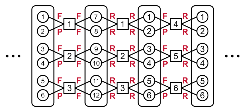
(a) Decoding succeeds.

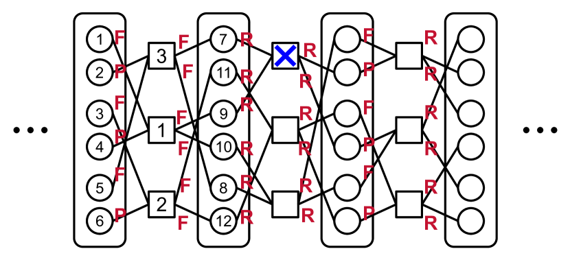
(b) Decoding fails.

Figure 2: An example where we decode the same encoding with different structures.

Figure 2 shows an example where we decode the same encoding with different structures. The first one (Figure 2(a)) succeeds; in fact, for the part shown in Figure 2(a), the resulting labeling satisfies all requirements of a valid labeling (Definition 3.11). The second one fails because for the square vertex (marked with an “x”), the two legs give conflicting labels: the first one labels it $3$ to close the edge $(\scalebox{0.85}{\footnotesize \leavevmode\hbox to13.13pt{\vbox to13.13pt{\text{[drawing]}}}},\scalebox{0.85}{\footnotesize \leavevmode\hbox to14.4pt{\vbox to14.4pt{\text{[drawing]}}}})$ while the second one labels it $1$ to close the edge $(\scalebox{0.85}{\footnotesize \leavevmode\hbox to13.13pt{\vbox to13.13pt{\text{[drawing]}}}},\scalebox{0.85}{\footnotesize \leavevmode\hbox to14.4pt{\vbox to14.4pt{\text{[drawing]}}}})$.

It is crucial that any valid labeling is captured by some encoding, so that we can bound the sum of labelings by the sum of encodings.

Lemma 3.18.

For any labeling $\sigma$ which is valid for some structure $\bm{\pi}\in(\widehat{\mathcal{S}}_{2t})^{2\ell}$, there is an encoding $\xi$ such that $\mathsf{Decode}(\xi,\bm{\pi})$ successfully outputs $\sigma$. Moreover, $\textsf{edge-factor}(\xi)\geqslant\textsf{edge-factor}(\sigma,\bm{\pi})$.

Proof.

Given a valid labeling for a structure, the $4t\ell$ leg types and the specification of vertices (a new vertex for $\mathsf{F}$, a previous location for $\mathsf{N}$, and an incident edge for $\mathsf{H}$) are straightforward to determine. For circle vertices, the bucket index $b\in[\log n]$ is specified such that the total number of edges incident to the vertex is between $2^{b}$ and $2^{b+1}$. Here $b\leqslant\log n$ since $4t\ell\ll 2^{\log n}=n$. In particular, the number of circle vertices in bucket $b$ is at most $\frac{4t\ell}{2^{b}}$.

The return labels are also straightforward. As shown in Lemma 3.17, one return label for each $\mathsf{N}$ or $\mathsf{H}$ is enough to guide all unforced returns. Thus, we can specify the return labels arriving at a vertex $v$ according to the ordering in which active edges incident to $v$ are closed. A circle vertex with bucket index $b$ has at most $2^{b+1}$ incident edges, whereas a square vertex has at most $4\ell$ incident edges (due to requirement 2 of Definition 3.11 that the square vertices in each block are distinct). For a square vertex $v$, two departing $\mathsf{R}$ legs are taken to close the final two active edges during the last visit to $v$. The return label for the $\mathsf{P}$ leg (an element in $\{1,2\}$) that initially creates $v$ is decided by the ordering of these final two $\mathsf{R}$ legs. Therefore, the ranges of return labels as defined in the encoding are sufficient.

For the edge factors, consider an edge traversed $2k\geqslant 2$ times in the walk. If the edge is created by an $\{\mathsf{F},\mathsf{P}_{2}\}$ pair, then as discussed in Remark 3.16, we may view the $\mathsf{P}_{2}$ leg as the third time the edge is traversed. In this case, the edge will be traversed by $1$ $\mathsf{F}$, $1$ $\mathsf{P}_{2}$, $(k-2)$ $\mathsf{H}$ and $k$ $\mathsf{R}$ legs. Then, the edge factor of $\xi$ from this edge will be $\mu_{4}\cdot(C\log n)^{k-2}$. This is a valid upper bound as $\mathbb{E}[a^{2k}]\leqslant\mathbb{E}[a^{4}]\cdot(\sqrt{C\log n})^{2k-4}\leqslant\mu_{4}\cdot(C\log n)^{k-2}$.

On the other hand, in other cases the edge will be traversed by $1$ $\mathsf{F}$, $(k-1)$ $\mathsf{H}$ and $k$ $\mathsf{R}$ legs, giving an edge factor of $(C\log n)^{k-1}$. This is also a valid upper bound as $\mathbb{E}[a^{2k}]\leqslant\mathbb{E}[a^{2}]\cdot(\sqrt{C\log n})^{2k-2}\leqslant(C\log n)^{k-1}$. Therefore, $\textsf{edge-factor}(\xi)$ as defined in Definition 3.15 is a valid upper bound on $\textsf{edge-factor}(\sigma,\bm{\pi})$. ∎

The next lemma states two simple but important relationships between the number of legs of each type in a valid encoding.

Lemma 3.19.

Let $\xi$ be an encoding such that $\mathsf{Decode}(\xi,\bm{\pi})$ succeeds for some $\bm{\pi}$. Let $\mathfrak{f}_{s},\mathfrak{p}_{s},\mathfrak{n}_{s},\mathfrak{h}_{s},\mathfrak{r}_{s}$ be the number of $\mathsf{F},\mathsf{P},\mathsf{N},\mathsf{H},\mathsf{R}$ legs from circle to square, let $\mathfrak{f}_{c},\mathfrak{n}_{c},\mathfrak{h}_{c},\mathfrak{r}_{c}$ be the number of $\mathsf{F},\mathsf{N},\mathsf{H},\mathsf{R}$ legs from square to circle, and let $\mathfrak{n}=\mathfrak{n}_{s}+\mathfrak{n}_{c}$, $\mathfrak{h}=\mathfrak{h}_{s}+\mathfrak{h}_{c}$ and $\mathfrak{r}=\mathfrak{r}_{s}+\mathfrak{r}_{c}$. Then, we must have

1. $\mathfrak{r}=2\mathfrak{f}_{s}+\mathfrak{f}_{c}+\mathfrak{n}+\mathfrak{h}=2t\ell$.

2. $\mathfrak{n}_{s}+\mathfrak{h}_{s}+\mathfrak{r}_{s}=\mathfrak{f}_{c}+\mathfrak{n}+\mathfrak{h}$.

Proof.

First, recall from the encoding (Definition 3.15) that each $\mathsf{P}$ must be paired with an $\mathsf{F}$ from circle to square, so $\mathfrak{p}_{s}=\mathfrak{f}_{s}$. Next, each $\mathsf{F}$, $\mathsf{P}$, $\mathsf{N}$ and $\mathsf{H}$ leg creates an active edge that needs to be closed by an $\mathsf{R}$ leg, thus

$$\mathfrak{r}=\mathfrak{f}+\mathfrak{p}_{s}+\mathfrak{n}+\mathfrak{h}=2\mathfrak{f}_{s}+\mathfrak{f}_{c}+\mathfrak{n}+\mathfrak{h}\,.$$ (7)

Next, the total number of edges is $4t\ell$, so $2\mathfrak{f}_{s}+\mathfrak{f}_{c}+\mathfrak{n}+\mathfrak{h}+\mathfrak{r}=4t\ell$, which means that $\mathfrak{r}=2\mathfrak{f}_{s}+\mathfrak{f}_{c}+\mathfrak{n}+\mathfrak{h}=2t\ell$.

Moreover, as the number of edges from circle to square is the same as that from square to circle, we have

$$2\mathfrak{f}_{s}+\mathfrak{n}_{s}+\mathfrak{h}_{s}+\mathfrak{r}_{s}=\mathfrak{f}_{c}+\mathfrak{n}_{c}+\mathfrak{h}_{c}+\mathfrak{r}_{c}\,.$$

Combined with Eq. 7, we get $\mathfrak{r}_{s}+\mathfrak{r}_{c}=2(\mathfrak{f}_{c}+\mathfrak{n}_{c}+\mathfrak{h}_{c})+(\mathfrak{r}_{c}-\mathfrak{r}_{s})$, which means $\mathfrak{r}_{s}=\mathfrak{f}_{c}+\mathfrak{n}_{c}+\mathfrak{h}_{c}$. Thus, $\mathfrak{n}_{s}+\mathfrak{h}_{s}+\mathfrak{r}_{s}=\mathfrak{f}_{c}+\mathfrak{n}+\mathfrak{h}$. ∎

We next prove the crucial lemma upper bounding the success probability of decoding over random permutations of the structure.

Lemma 3.20 (Decoding success probability).

Let $\xi$ be an encoding, let $\mathfrak{f}_{c}$ be the number of $\mathsf{F}$ legs from square to circle, and let $\mathfrak{n},\mathfrak{h}$ be the number of $\mathsf{N},\mathsf{H}$ legs. Then,

$$\mathop{\bf Pr\/}_{\bm{\pi}\sim(\widehat{\mathcal{S}}_{2t})^{2\ell}}\left[\text{$\mathsf{Decode}(\xi,\bm{\pi})$ succeeds}\right]\leqslant\left\lparen\frac{t}{e}\right\rparen^{-\frac{1}{2}(\mathfrak{f}_{c}+\mathfrak{n}+\mathfrak{h})}\,.$$

Proof.

Let $\mathfrak{f}_{s},\mathfrak{p}_{s},\mathfrak{n}_{s},\mathfrak{h}_{s},\mathfrak{r}_{s}$ be the number of $\mathsf{F},\mathsf{P},\mathsf{N},\mathsf{H},\mathsf{R}$ legs from circle to square, and let $\mathfrak{f}_{c},\mathfrak{n}_{c},\mathfrak{h}_{c},\mathfrak{r}_{c}$ be the number of $\mathsf{F},\mathsf{N},\mathsf{H},\mathsf{R}$ legs from square to circle. Consider the circle-to-square part of each block, and view the structure as a perfect matching between $2t$ circle vertices. The $\mathsf{F}$ and $\mathsf{P}$ legs must be paired and the $t$ square vertices must receive distinct labels. Moreover, all $\mathsf{N},\mathsf{H},\mathsf{R}$ legs from circle to square provide labels, and recall that Algorithm 1 fails if any square vertex receives two different labels. Therefore, there is exactly one way to pair up all the $\mathsf{N},\mathsf{H},\mathsf{R}$ legs.

Suppose there are $i\leqslant t$ number of $\mathsf{F}$, $i$ number of $\mathsf{P}$ (because $\mathsf{F}$ and $\mathsf{P}$ must be paired), and $2t-2i$ other legs. There are $(2t-1)!!\geqslant(\frac{2t}{e})^{t}$ number of ways to group them into pairs. However, there are $i!$ ways to pair the $\mathsf{F}$ and $\mathsf{P}$ legs, and there is a unique way to pair the other legs. Thus, via Stirling’s approximation, the probability that a grouping is valid is

$$\frac{i!}{(2t-1)!!}\leqslant i!\left\lparen\frac{2t}{e}\right\rparen^{-t}\leqslant\left\lparen\frac{t}{e}\right\rparen^{-(t-i)}\,.$$

Note that $t-i$ is $1/2$ of the number of $\mathsf{N},\mathsf{H}$ and $\mathsf{R}$ legs from circle to square in the block. Thus, overall, the probability of success is upper bounded by $(t/e)^{-\frac{1}{2}(\mathfrak{n}_{s}+\mathfrak{h}_{s}+\mathfrak{r}_{s})}$. By Lemma 3.19, we have $\mathfrak{n}_{s}+\mathfrak{h}_{s}+\mathfrak{r}_{s}=\mathfrak{f}_{c}+\mathfrak{n}+\mathfrak{h}$, thus completing the proof. ∎

3.5 Proof of Lemma 3.9

We can finally finish the proof of Lemma 3.9.

Proof of Lemma 3.9.

We start with writing the trace as a sum of encodings:

$$\mathbb{E}_{A}\operatorname{tr}\left\lparen\widetilde{M}^{\ell}\right\rparen \leqslant\mathbb{E}_{\bm{\pi}\sim(\widehat{\mathcal{S}}_{2t})^{2\ell}}\sum_{\sigma:\text{ labeling}}\bm{1}(\text{$\sigma$ valid for $\bm{\pi}$})\cdot\textsf{edge-factor}(\sigma,\bm{\pi})$$

$$\leqslant\mathbb{E}_{\bm{\pi}\sim(\widehat{\mathcal{S}}_{2t})^{2\ell}}\sum_{\sigma:\text{ labeling}}\sum_{\xi:\text{ encoding}}\bm{1}(\mathsf{Decode}(\xi,\bm{\pi})=\sigma\text{ \& valid for $\bm{\pi}$})\cdot\textsf{edge-factor}(\xi)$$

$$\leqslant\sum_{\xi:\text{ encoding}}\mathop{\bf Pr\/}_{\bm{\pi}\sim(\widehat{\mathcal{S}}_{2t})^{2\ell}}\left[\text{$\mathsf{Decode}(\xi,\bm{\pi})$ succeeds}\right]\cdot\textsf{edge-factor}(\xi)\,.$$

Here, the second inequality follows from Lemma 3.18 that every labeling $\sigma$ has an encoding $\xi$ such that $\mathsf{Decode}(\xi,\bm{\pi})$ successfully outputs $\sigma$, and that $\textsf{edge-factor}(\sigma,\bm{\pi})\leqslant\textsf{edge-factor}(\xi)$.

We bound the number of encodings as follows:

• For each $\{\mathsf{F},\mathsf{P}\}$ leading to a square, there are $n$ choices for the new vertex, and $2$ choices for the return label of $\mathsf{P}$. In total, $2n$ choices.

• For each $\mathsf{F}$ from square to circle, there are $d$ choices for the new vertex and $\log n$ choices for the bucket index. In total, $d\log n$ choices.

• For each $\mathsf{N}$ from circle to square, there are $t\ell$ choices for a previous square vertex, and $4\ell$ choices for the return label. In total, $4t\ell^{2}$ choices.

• For each $\mathsf{N}$ or $\mathsf{H}$ from square to circle, there are $\log n$ choices to choose a bucket index $b$, and $\frac{4t\ell}{2^{b}}$ choices for a vertex in bucket $b$. Then, there are $2^{b+1}$ choices for a return label. In total, $\log n\cdot\frac{4t\ell}{2^{b}}\cdot 2^{b+1}=8t\ell\log n$ choices.

• For each $\mathsf{H}$ from circle to square, there are $4t\ell$ choices to choose an incident edge, and $4\ell$ choices for a return label. In total, $16t\ell^{2}$ choices.

• Edge factor: Each $\mathsf{H}$ gets a $C\log n$ factor, and each $\mathsf{P}_{2}$ gets a $\mu_{4}$ factor. Recall that $\mu_{4}$ and $C$ are the constants such that $\mathbb{E}[a_{ij}^{4}]\leqslant\mu_{4}$ and $|a_{ij}|\leqslant\sqrt{C\log n}$ almost surely.

Fix a leg type pattern and starting index in $[d]^{2t}$ (labels for the first $2t$ circle vertices in the structure), and let $\mathfrak{f}_{s},\mathfrak{p}_{s},\mathfrak{n}_{s},\mathfrak{h}_{s},\mathfrak{r}_{s}$ be the number of $\mathsf{F},\mathsf{P},\mathsf{N},\mathsf{H},\mathsf{R}$ legs from circle to square, and let $\mathfrak{f}_{c},\mathfrak{n}_{c},\mathfrak{h}_{c},\mathfrak{r}_{c}$ be the number of $\mathsf{F},\mathsf{N},\mathsf{H},\mathsf{R}$ legs from square to circle. Moreover, let $\mathfrak{n}=\mathfrak{n}_{s}+\mathfrak{n}_{c}$ and $\mathfrak{h}=\mathfrak{h}_{s}+\mathfrak{h}_{c}$. Then, the total encodings, weighted by edge-factor, is bounded by

$$\begin{gathered}n^{\mathfrak{f}_{s}}(2\mu_{4})^{\mathfrak{p}_{s}}(d\log n)^{\mathfrak{f}_{c}}(4t\ell^{2})^{\mathfrak{n}_{s}}(8t\ell\log n)^{\mathfrak{n}_{c}}(16Ct\ell^{2}\log n)^{\mathfrak{h}_{s}}(8Ct\ell\log^{2}n)^{\mathfrak{h}_{c}}\\ \leqslant(2\mu_{4}n)^{\mathfrak{f}_{s}}(d\log n)^{\mathfrak{f}_{c}}(8t\log^{2}n)^{\mathfrak{n}}(16Ct\log^{3}n)^{\mathfrak{h}}\,,\end{gathered}$$

where we use the fact that $\mathfrak{p}_{s}=\mathfrak{f}_{s}$, $\mu_{4}\geqslant 1$ and $\ell\leqslant\log n$.

Next, by Lemma 3.20, $\mathop{\bf Pr\/}_{\bm{\pi}}[\mathsf{Decode}(\xi,\bm{\pi})\text{ succeeds}]\leqslant(t/e)^{-\frac{1}{2}(\mathfrak{f}_{c}+\mathfrak{n}+\mathfrak{h})}$. Thus, we get

$$(2\mu_{4}n)^{\mathfrak{f}_{s}}\left\lparen\sqrt{\frac{e}{t}}d\log n\right\rparen^{\mathfrak{f}_{c}}O\left\lparen\sqrt{t}\log^{3}n\right\rparen^{\mathfrak{n}+\mathfrak{h}}\leqslant O\left\lparen\mu_{4}n+\frac{d^{2}}{t}\log^{2}n\right\rparen^{\mathfrak{f}_{s}+\frac{1}{2}\mathfrak{f}_{c}}O\left\lparen\sqrt{t}\log^{3}n\right\rparen^{\mathfrak{n}+\mathfrak{h}}$$

By Lemma 3.19, $2\mathfrak{f}_{s}+\mathfrak{f}_{c}=2t\ell-\mathfrak{n}-\mathfrak{h}$. Thus, as long as $t\log^{6}n\leqslant\mu_{4}n+\frac{d^{2}}{t}\log^{2}n$, the above is bounded by $O(\mu_{4}n+\frac{d^{2}}{t}\log^{2}n)^{t\ell}$.

Finally, there are at most $2^{O(t\ell)}$ leg type patterns, and $d^{2t}$ choices for the starting index $J\in[d]^{2t}$ in the encoding. This gives the final bound of $d^{2t}\cdot O(\mu_{4}n+\frac{d^{2}}{t}\log^{2}n)^{t\ell}$. ∎

4 Planted Sparse Vector

We first restate the planted sparse vector model.

Model (Restatement of Model 1).

Fix an unknown unit vector $v\in\mathbb{R}^{n}$, and let $d\leqslant n\in\mathbb{N}$. Let $\widetilde{A}$ be a random $n\times d$ matrix sampled as follows: (1) let $A$ be the random matrix such that the first column is $v$ and the other $d-1$ columns are i.i.d. $\mathcal{N}(0,\frac{1}{n}\mathbb{I}_{n})$ vectors; (2) let $R\in\mathbb{R}^{d\times d}$ be an arbitrary unknown rotation matrix; (3) set $\widetilde{A}=AR$.

The task is that given $\widetilde{A}$, output a unit vector $\widehat{v}\in\mathbb{R}^{n}$ such that $\langle\widehat{v},v\rangle^{2}\geqslant 1-o(1)$.

We first characterize the sparse vectors that we will plant in Model 1. Motivated by the definition of well-spread subspaces (Definition 3.1), we define the notion of compressible vectors as follows,

Definition 4.1 (Compressible vector).

Let $\rho,\gamma\in(0,1)$. We say that a vector $v\in\mathbb{R}^{n}$ is $(\rho,\gamma)$-compressible if

$$\max_{S\subseteq[n]:|S|\leqslant\rho n}\left\lVert v_{S}\right\rVert_{2}=(1-\gamma)\lVert v\rVert_{2}\,.$$

In other words, $v$ is compressible if the top $\rho n$ coordinates of $v$ contains $1-\gamma$ fraction of its $\ell_{2}$-mass.

Next, recall our notation for the elementary symmetric polynomial (of the 4th powers):

$$Q_{t}(z)\coloneqq t!\sum_{S\subseteq[n]:|S|=t}\prod_{i\in S}z_{i}^{4}\,.$$

We now state our main result.

Theorem 4.2 (Formal version of 2).

There is an absolute positive constant $C$ such that for every $t\leqslant d\leqslant n\in\mathbb{N}$ such that $\frac{\rho d^{2}}{n}\log^{C}n\leqslant t\leqslant\frac{d}{\log^{C}n}$ and $\rho\in(0,\frac{1}{\log^{C}n})$, there is a randomized algorithm with running time $2^{\widetilde{O}(t)}$ with the following guarantee: Given $\widetilde{A}\in\mathbb{R}^{n\times d}$ drawn from Model 1 with a hidden unit vector $v\in\mathbb{R}^{n}$ such that $v$ is $(\rho,1/2)$-compressible and $Q_{t}(v)^{1/t}\geqslant(1-\frac{1}{\log^{C}n})\|v\|_{4}^{4}$, the algorithm outputs a unit vector $\widehat{v}\in\operatorname{colspan}(\widetilde{A})$ such that $\langle\widehat{v},v\rangle^{2}\geqslant 1-o(1)$ with probability $1-o(1)$ over the randomness of the algorithm and the input.

To interpret the parameters in Theorem 4.2, consider $d=O(n^{\frac{1+\varepsilon}{2}})$ and $t=\widetilde{O}(n^{\varepsilon})$ (same as in Theorem 3.3), and the sparsity of $v$ is $\rho=1/\operatorname{polylog}(n)$. Then, we can approximately recover $v$ in $2^{\widetilde{O}(n^{\varepsilon})}$ time. This establishes the same trade-off between the dimension and runtime as our certification algorithm (1).

Our algorithm is described in Algorithm 2, and the proof of Theorem 4.2 is completed at the end of Section 4.3.

Remark 4.3 (Assumptions on $v$).

The assumption that $Q_{t}(v)^{1/t}\geqslant(1-o(1))\|v\|_{4}^{4}$ is not standard. In particular, this does not hold for any vector $v$ whose mass concentrates on $<t$ coordinates. However, for such vectors, one can simply brute-force search over all support of size $\leqslant\widetilde{O}(t)$, which takes $2^{\widetilde{O}(t)}$ time.

On the other hand, most distributions of sparse vectors used in previous works satisfy that $Q_{t}(v)^{1/t}\geqslant(1-o(1))\|v\|_{4}^{4}$ (when the sparsity is not small enough to brute-force search over the support). These include the noiseless and noisy Rademacher-Bernoulli distribution (Definition 1.1) considered in [MW21, Cd22, DK22, ZSWB22] and the Rademacher-Gaussian distribution considered in [MW21].

We note that the algorithms of [HSSS16, MW21] require very minimal assumptions on $v$. In particular, the algorithm of [MW21] succeeds as long as $\left\lvert\|v\|_{4}^{4}-\frac{3}{n}\right\rvert\geqslant\Omega(\frac{1}{n})$ and $\frac{1}{\|v\|_{4}^{4}}\frac{d}{n^{3/2}}\ll 1$, so when $\|v\|_{4}^{4}\approx\frac{1}{\rho n}$, this is equivalent to $\rho d\ll\sqrt{n}$. We leave as future work the identification of a minimal analytic assumption on $v$ that ensures successful recovery in the subexponential-time regime.

4.1 Preliminaries for the planted sparse vector model

It is easy to see that a compressible vector $v$ has large $4$-norm:

Lemma 4.4.

A $(\rho,\gamma)$-compressible vector $v\in\mathbb{R}^{n}$ satisfies $\|v\|_{4}^{4}\geqslant\frac{(1-\gamma)^{4}}{\rho n}\|v\|_{2}^{2}$.

Proof.

Let $S^{*}\subseteq[n]$ be such that $|S^{*}|\leqslant\rho n$ and $\|v_{S^{*}}\|_{2}\geqslant(1-\gamma)\|v\|_{2}$. Then, by Cauchy-Schwarz, $(1-\gamma)^{4}\|v\|_{2}^{4}\leqslant\|v_{S^{*}}\|_{2}^{4}\leqslant|S|\cdot\|v_{S}\|_{4}^{4}\leqslant\rho n\cdot\|v\|_{4}^{4}$. ∎

The following lemma is also straightforward given the standard singular value concentration bounds on Gaussian matrices (Fact 3.5).

Lemma 4.5.

Let $d\leqslant n/\operatorname{polylog}(n)$. Let $A\in\mathbb{R}^{n\times d}$ be drawn from Model 1 with an arbitrary unit vector $v$. Then, with probability $1-o(1)$, we have $1-o(1)\leqslant\sigma_{\min}(A)\leqslant\sigma_{\max}(A)\leqslant 1+o(1)$.

Proof.

Recall that the first column of $A$ is $v$, and let $\overline{A}\in\mathbb{R}^{n\times(d-1)}$ be the rest of the matrix with i.i.d. $\mathcal{N}(0,1/n)$ entries. By Fact 3.5, we know that $\sigma_{\max}(\overline{A})\leqslant 1+o(1)$ with high probability. Moreover, since $v$ is a unit vector, $\overline{A}^{\top}v$ is distributed as a $(d-1)$-dimensional vector with $\mathcal{N}(0,1/n)$ entries, thus with high probability we have $\|\overline{A}^{\top}v\|_{2}^{2}\leqslant O(d/n)\leqslant o(1)$.

For any unit vector $x=(x_{1},\overline{x})$, we have $Ax=x_{1}v+\overline{A}\overline{x}$, thus

$$\|Ax\|_{2}^{2} =x_{1}^{2}\|v\|_{2}^{2}+\left\lVert\overline{A}\overline{x}\right\rVert_{2}^{2}+2x_{1}v^{\top}\overline{A}\overline{x}\leqslant x_{1}^{2}\|v\|_{2}^{2}+\left\lVert\overline{A}\overline{x}\right\rVert_{2}^{2}+2|x_{1}|\|\overline{x}\|_{2}\left\lVert\overline{A}^{\top}v\right\rVert_{2}$$

$$\leqslant(1+o(1))\left\lparen x_{1}^{2}+\left\lVert\overline{x}\right\rVert_{2}^{2}\right\rparen=(1+o(1))\lVert x\rVert_{2}^{2}\,.$$

Similarly, the minimum singular value lower bound follows from the fact that $\sigma_{\min}(\overline{A})\geqslant 1-o(1)$ and $\|Ax\|_{2}^{2}\geqslant x_{1}^{2}\|v\|_{2}^{2}+\|\overline{A}\overline{x}\|_{2}^{2}-2|x_{1}|\|\overline{x}\|_{2}\lVert\overline{A}^{\top}v\rVert_{2}$. ∎

The following lemma is important in our algorithm to identify a “good” vector to output.

Lemma 4.6.

Let $n,d\in\mathbb{N}$ such that $d\leqslant n/\operatorname{polylog}(n)$, let $\rho\leqslant 1/\operatorname{polylog}(n)$, and let $\gamma,\delta\in(0,1)$. Let $v\in\mathbb{R}^{n}$ be a $(\rho,\gamma)$-compressible unit vector, and let $A\in\mathbb{R}^{n\times d}$ be drawn from Model 1 with planted vector $v$. Then, with probability $1-o(1)$ over $A$, the following holds: let $y\in\mathbb{R}^{d}$ be any unit vector and let $\widehat{v}=Ay$,

1. If $\|y-e_{1}\|_{2}\leqslant\delta$ or $\|y+e_{1}\|_{2}\leqslant\delta$, then $\max_{S:|S|\leqslant\rho n}\|\widehat{v}_{S}\|_{2}\geqslant 1-\gamma-(1+o(1))\delta$.

2. If $\|y-e_{1}\|_{2}\geqslant\delta$ and $\|y+e_{1}\|_{2}\geqslant\delta$, then $\max_{S:|S|\leqslant\rho n}\|\widehat{v}_{S}\|_{2}\leqslant(1-\frac{1}{2}\delta^{2})(1-\gamma)+\frac{1}{\operatorname{polylog}(n)}$.

Proof.

Let $S^{*}=\operatorname*{arg\,max}_{S:|S|\leqslant\rho n}\|v_{S}\|_{2}$, and recall that $Ae_{1}=v$.

Suppose $\|y-e_{1}\|_{2}\leqslant\delta$. Then, $\|\widehat{v}-v\|_{2}=\|A(y-e_{1})\|_{2}\leqslant\sigma_{\max}(A)\delta\leqslant(1+o(1))\delta$ with high probability by Lemma 4.5. By the triangle inequality, $\|\widehat{v}_{S^{*}}\|_{2}\geqslant\|v_{S^{*}}\|_{2}-\|v_{S^{*}}-\widehat{v}_{S^{*}}\|_{2}\geqslant 1-\gamma-(1+o(1))\delta$ since $\|v_{S^{*}}-\widehat{v}_{S^{*}}\|_{2}\leqslant\|v-\widehat{v}\|_{2}\leqslant(1+o(1))\delta$. The same is true if we flip the sign of $y$ so that $\widehat{v}$ is close to $-v$. This proves the first statement.

Suppose $\|y-e_{1}\|_{2}\geqslant\delta$ and $\|y+e_{1}\|_{2}\geqslant\delta$. Denote $y=(y_{1},\overline{y})$, where $\overline{y}\in\mathbb{R}^{d-1}$ and $\lVert\overline{y}\rVert_{2}^{2}=1-y_{1}^{2}$. Then, we have $\delta^{2}\leqslant(1-y_{1})^{2}+\lVert\overline{y}\rVert_{2}^{2}=2-2y_{1}$ and $\delta^{2}\leqslant(1+y_{1})^{2}+\lVert\overline{y}\rVert_{2}^{2}=2+2y_{1}$, which means that $|y_{1}|\leqslant 1-\delta^{2}/2$. For any $S\subseteq[n]$ with $|S|\leqslant\rho n$, we have $\sigma_{\max}(\overline{A}_{S})\leqslant\widetilde{O}(\sqrt{d/n}+\sqrt{\rho})\leqslant 1/\operatorname{polylog}(n)$ by Fact 3.5 and a union bound over all $S$ (here we need $\rho,d/n\leqslant\frac{1}{\operatorname{polylog}(n)}$). Then, since $\widehat{v}_{S}=y_{1}v_{S}+\overline{A}_{S}\overline{y}$, by the triangle inequality, $\|\widehat{v}_{S}\|_{2}\leqslant|y_{1}|\lVert v_{S}\rVert_{2}+\left\lVert\overline{A}_{S}\overline{y}\right\rVert_{2}\leqslant(1-\frac{1}{2}\delta^{2})\lVert v_{S^{*}}\rVert_{2}+\frac{1}{\operatorname{polylog}(n)}$, which proves the second statement. ∎

4.2 Background on Sum-of-Squares

In this section, we give an overview of the Sum-of-Squares (SoS) framework. We refer the reader to the monograph [FKP19] and the lecture notes [BS16] for a detailed exposition of the SoS method and its usage in algorithm design.

Pseudo-distributions.

Pseudo-distributions are generalizations of probability distributions and are represented by their pseudo-expectation operators. Formally, a degree-$t$ pseudo-distribution $\mu$ over variables $x_{1},,\dots,x_{n}$ corresponds to a linear operator $\widetilde{\mathbb{E}}_{\mu}$ that maps polynomials of degree $\leqslant t$ to real numbers and satisfies $\widetilde{\mathbb{E}}_{\mu}[1]=1$ and $\widetilde{\mathbb{E}}_{\mu}[p^{2}]\geqslant 0$ for every polynomial $p(x_{1},\ldots,x_{n})$ of degree $\leqslant t/2$.

Let $\mathcal{A}=\{f_{1}\geqslant 0,f_{2}\geqslant 0,\dots,f_{m}\geqslant 0\}$ be a system of $m$ polynomial inequality constraints. We say that $\mu$ satisfies the system of constraints $\mathcal{A}$ at degree $t$ if for every sum-of-squares polynomial $h$ and any $T\subseteq[m]$ such that $\deg(h)+\sum_{i\in T}\deg(f_{i})\leqslant t$, $\widetilde{\mathbb{E}}_{\mu}[h\cdot\prod_{i\in T}f_{i}]\geqslant 0$. In particular, if $\mathcal{A}$ contains an equality constraint $f=0$, then $\widetilde{\mathbb{E}}_{\mu}[f\cdot p]=0$ for any polynomial $p$ with $\deg(f)+\deg(p)\leqslant t$. Specific to our application, we say that a pseudo-distribution $\mu$ satisfies the unit sphere constraints if $\widetilde{\mathbb{E}}_{\mu}[\lVert x\rVert_{2}^{2}\cdot p(x)]=\widetilde{\mathbb{E}}_{\mu}[p(x)]$ for every $p$ of degree $\leqslant t-2$.

Unlike true distributions, there is a $n^{O(t)}$-time weak separation oracle for degree-$t$ pseudo-distributions, which allows us to efficiently optimize over pseudo-distributions that satisfy a given set of polynomial constraints (approximately) via the ellipsoid method — this is called the Sum-of-Squares algorithm. Therefore, given a polynomial $p$ (with the $\ell_{1}$-norm of the coefficients being $\lVert p\rVert_{1}$) over $x_{1},\dots,x_{n}$, a degree-$t$ pseudo-distribution satisfying the unit sphere constraint that maximizes $p$ within an additive $\varepsilon\lVert p\rVert_{1}$ error can be found in time $n^{O(t)}\operatorname{polylog}(n/\varepsilon)$.

Sum-of-Squares proofs.

Let $f_{1},f_{2},\dots,f_{m}$ and $g$ be multivariate polynomials in $x$. A sum-of-squares proof that the constraints $\mathcal{A}=\{f_{1}\geqslant 0,\dots,f_{m}\geqslant 0\}$ imply $g\geqslant 0$ consists of sum-of-squares polynomials $(p_{S})_{S\subseteq[m]}$ such that $g(x)=\sum_{S\subseteq[m]}p_{S}(x)\prod_{i\in S}f_{i}(x)$. The degree of such an SoS proof equals the maximum of the degree of $p_{S}\prod_{i\in S}f_{i}$ over all $S$ appearing in the sum above. We write

$$\mathcal{A}\mathrel{\leavevmode\hbox{\set@color\raisebox{3.44444pt}{$\rule[-6.45831pt]{0.47787pt}{12.91663pt}\rule[-0.23894pt]{8.00063pt}{0.47787pt}\raisebox{-6.26668pt}{\makebox[8.00063pt]{\leavevmode\hbox{\set@color$\scriptstyle{t}$}}}\raisebox{1.96112pt}{\makebox[8.00063pt]{\leavevmode\hbox{\set@color$\scriptstyle{x}$}}}$}}}\{g(x)\geqslant 0\}$$

where $t$ is the degree of the SoS proof.

The following fact is the crucial connection between SoS proofs and pseudo-distributions.

Fact 4.7.

Suppose $\mathcal{A}\mathrel{\leavevmode\hbox{\set@color\raisebox{3.44444pt}{$\rule[-6.45831pt]{0.47787pt}{12.91663pt}\rule[-0.23894pt]{8.00063pt}{0.47787pt}\raisebox{-6.26668pt}{\makebox[8.00063pt]{\leavevmode\hbox{\set@color$\scriptstyle{t}$}}}\raisebox{1.96112pt}{\makebox[8.00063pt]{\leavevmode\hbox{\set@color$\scriptstyle{x}$}}}$}}}\{g(x)\geqslant 0\}$ for some polynomial constraints $\mathcal{A}$ and a polynomial $g$. Let $\mu$ be any pseudo-distribution of degree $\geqslant t$ satisfying $\mathcal{A}$. Then, $\widetilde{\mathbb{E}}_{\mu}[g]\geqslant 0$.

In other words, for polynomials $f,g$, in order to prove that $\widetilde{\mathbb{E}}_{\mu}[f]\leqslant\widetilde{\mathbb{E}}_{\mu}[g]$ for any degree-$t$ pseudo-distribution $\mu$ satisfying $\mathcal{A}$, it suffices to show an SoS proof that $\mathcal{A}\mathrel{\leavevmode\hbox{\set@color\raisebox{3.44444pt}{$\rule[-6.45831pt]{0.47787pt}{12.91663pt}\rule[-0.23894pt]{8.00063pt}{0.47787pt}\raisebox{-6.26668pt}{\makebox[8.00063pt]{\leavevmode\hbox{\set@color$\scriptstyle{t}$}}}\raisebox{1.96112pt}{\makebox[8.00063pt]{\leavevmode\hbox{\set@color$\scriptstyle{x}$}}}$}}}\{f(x)\leqslant g(x)\}$.

We will need the following SoS versions of Cauchy-Schwarz and Hölder’s inequalities.

Fact 4.8 (Fact 3.9 and 3.11 in [OZ13]).

For any $\delta>0$,

• $\mathrel{\leavevmode\hbox{\set@color\raisebox{3.44444pt}{$\rule[-6.45831pt]{0.47787pt}{12.91663pt}\rule[-0.23894pt]{13.62817pt}{0.47787pt}\raisebox{-6.47223pt}{\makebox[13.62817pt]{\leavevmode\hbox{\set@color$\scriptstyle{2}$}}}\raisebox{3.32222pt}{\makebox[13.62817pt]{\leavevmode\hbox{\set@color$\scriptstyle{x,y}$}}}$}}}\left\{xy\leqslant\frac{\delta}{2}x^{2}+\frac{1}{2\delta}y^{2}\right\}$.

• $\mathrel{\leavevmode\hbox{\set@color\raisebox{3.44444pt}{$\rule[-6.45831pt]{0.47787pt}{12.91663pt}\rule[-0.23894pt]{13.62817pt}{0.47787pt}\raisebox{-6.47223pt}{\makebox[13.62817pt]{\leavevmode\hbox{\set@color$\scriptstyle{4}$}}}\raisebox{3.32222pt}{\makebox[13.62817pt]{\leavevmode\hbox{\set@color$\scriptstyle{x,y}$}}}$}}}\left\{x^{3}y\leqslant\frac{3\delta}{4}x^{4}+\frac{1}{4\delta^{3}}y^{4}\right\}$.

Using Fact 4.8, we can prove the following lemma, which is basically the SoS version of Jensen’s inequality applied to the $x^{4}$ function.

Lemma 4.9.

For any $\delta>0$,

$$\mathrel{\leavevmode\hbox{\set@color\raisebox{3.44444pt}{$\rule[-6.45831pt]{0.47787pt}{12.91663pt}\rule[-0.23894pt]{13.62817pt}{0.47787pt}\raisebox{-6.47223pt}{\makebox[13.62817pt]{\leavevmode\hbox{\set@color$\scriptstyle{4}$}}}\raisebox{3.32222pt}{\makebox[13.62817pt]{\leavevmode\hbox{\set@color$\scriptstyle{x,y}$}}}$}}}\left\{(x+y)^{4}\leqslant(1+\delta)^{3}\left\lparen x^{4}+\frac{y^{4}}{\delta^{3}}\right\rparen\right\}\,.$$

Proof.

We expand $(x+y)^{4}=x^{4}+4x^{3}y+6x^{2}y^{2}+4xy^{3}+y^{4}$ and apply Fact 4.8 to the middle 3 terms: $(x+y)^{4}\leqslant x^{4}+(3\delta x^{4}+\frac{1}{\delta^{3}}y^{4})+(3\delta^{2}x^{4}+\frac{3}{\delta^{2}}y^{4})+(\delta^{3}x^{4}+\frac{3}{\delta}y^{4})+y^{4}=(1+\delta)^{3}x^{4}+(1+\frac{1}{\delta})^{3}y^{4}$. ∎

Rounding.

In the following, we state an important technique for rounding pseudo-distributions from [BKS15].

Lemma 4.10 (Theorem 5.1 of [BKS15]).

For every even $t\in\mathbb{N}$ and $\varepsilon\in(0,1)$, there exists a randomized algorithm with running time $n^{O(t)}$ and success probability $2^{-t/\operatorname{poly}(\varepsilon)}$ for the following problem: Fix an unknown unit vector $q\in\mathbb{R}^{n}$. Given a degree-$t$ pseudo-distribution $\mu$ over $x\in\mathbb{R}^{n}$ satisfying the constraint $\|x\|_{2}^{2}=1$ such that $\widetilde{\mathbb{E}}_{\mu}[\langle q,x\rangle^{t}]\geqslant e^{-\varepsilon t}$, output a unit vector $\widehat{x}\in\mathbb{R}^{n}$ with $\langle q,\widehat{x}\rangle\geqslant 1-O(\varepsilon)$.

4.3 Algorithm for planted sparse vector

Algorithm 2 (Recover hidden sparse vector).

Input: A matrix $\widetilde{A}\in\mathbb{R}^{n\times d}$ drawn from Model 1, parameters $t\in\mathbb{N}$ and $\rho\in(0,1)$. Output: A unit vector $\widehat{v}\in\operatorname{colspan}(\widetilde{A})$. Operation: 1. Solve the degree-$4t$ SoS relaxation of the following program over $x\in\mathbb{R}^{d}$; $\displaystyle\max$ $\displaystyle\widetilde{P}_{t}(x)\coloneqq t!\sum_{S\subseteq[n]:|S|=t}\prod_{i\in S}\left\langle\widetilde{a}_{i},x\right\rangle^{4}$ s.t. $\displaystyle\|x\|_{2}^{2}=1$ where $\widetilde{a}_{1},\dots,\widetilde{a}_{n}$ are the rows in $\widetilde{A}$. 2. Repeat the algorithm of Lemma 4.10 $N=2^{\widetilde{O}(t)}$ times and obtain unit vectors $\widehat{x}^{(1)},\widehat{x}^{(2)},\dots,\widehat{x}^{(N)}$. 3. Let $\widehat{v}^{(i)}=\widetilde{A}\widehat{x}^{(i)}$, and let $j=\operatorname*{arg\,max}_{i\in[N]}\max_{S\subseteq[n]:|S|\leqslant\rho n}\lVert\widehat{v}^{(i)}_{S}\rVert_{2}$, i.e., the vector whose top $\rho n$ entries have the largest norm. Output $\widehat{v}^{(j)}/\|\widehat{v}^{(j)}\|_{2}$.

The main ingredient in the analysis is Lemma 3.6. Below, we state it as a degree-$4t$ SoS proof.

Lemma 4.11 (SoS version of Lemma 3.6).

Let $t\leqslant d\leqslant n$ be integers such that $t\log^{6}n\leqslant n+\frac{d^{2}}{t}\log^{2}n$. Let $A\sim\mathcal{N}(0,\frac{1}{n})^{n\times d}$ with rows $a_{1},\dots,a_{n}\in\mathbb{R}^{d}$. Then, with probability $1-\frac{1}{\operatorname{poly}(n)}$ over $a_{1},\dots,a_{n}$,

$$\mathrel{\leavevmode\hbox{\set@color\raisebox{3.44444pt}{$\rule[-6.45831pt]{0.47787pt}{12.91663pt}\rule[-0.23894pt]{10.02773pt}{0.47787pt}\raisebox{-6.47223pt}{\makebox[10.02773pt]{\leavevmode\hbox{\set@color$\scriptstyle{4t}$}}}\raisebox{3.32222pt}{\makebox[10.02773pt]{\leavevmode\hbox{\set@color$\scriptstyle{y}$}}}$}}}\left\{P_{t}(y)\coloneqq t!\sum_{S\subseteq[n]:|S|=t}\prod_{i\in S}\left\langle a_{i},y\right\rangle^{4}\leqslant O\left\lparen\frac{1}{n}+\frac{d^{2}}{n^{2}t}\log^{2}n\right\rparen^{t}\lVert y\rVert_{2}^{4t}\right\}\,.$$

Note the scaling of $1/n$ here because we assume the entries to be $\mathcal{N}(0,1/n)$ as opposed to $\mathcal{N}(0,1)$ in Lemma 3.6.

Using Lemma 4.11, we prove our main lemma.

Lemma 4.12.

Assume the same setting as Theorem 4.2. Let $r_{1}\in\mathbb{R}^{d}$ be the first row of the unknown rotation matrix $R$. Further, let $\mu$ be the degree-$4t$ pseudo-distribution over $x\in\mathbb{R}^{n}$ with the unit sphere constraint that maximizes $\widetilde{P}_{t}(x)$. Then, $\widetilde{\mathbb{E}}_{\mu}[\langle r_{1},x\rangle^{2t}]\geqslant e^{-O(t/\log n)}$.

Proof.

Recall from Model 1 that $\widetilde{A}=AR$ and $v$ is the first column of $A$. Denote $y=Rx$ such that $\langle\widetilde{a}_{i},x\rangle=\langle a_{i},Rx\rangle=\langle a_{i},y\rangle$ and $\widetilde{P}_{t}(x)=P_{t}(y)$. Note also that $y_{1}=\langle r_{1},x\rangle$. Our goal is to prove that $\widetilde{\mathbb{E}}_{\mu}[y_{1}^{2t}]$ is large.

For each row $a_{i}$ in $A$, we write $a_{i}=(v_{i},\overline{a}_{i})$, and for simplicity denote $w_{i}\coloneqq\langle\overline{a}_{i},\overline{y}\rangle$ such that $\langle a_{i},y\rangle=y_{1}v_{i}+w_{i}$. We first apply Lemma 4.9 with $\delta\coloneqq\frac{1}{\log^{3}n}$ to each $(y_{1}v_{i}+w_{i})^{4}$:

$$\mathrel{\leavevmode\hbox{\set@color\raisebox{3.44444pt}{$\rule[-6.45831pt]{0.47787pt}{12.91663pt}\rule[-0.23894pt]{10.02773pt}{0.47787pt}\raisebox{-6.47223pt}{\makebox[10.02773pt]{\leavevmode\hbox{\set@color$\scriptstyle{4t}$}}}\raisebox{3.32222pt}{\makebox[10.02773pt]{\leavevmode\hbox{\set@color$\scriptstyle{y}$}}}$}}}\left\{P_{t}(y)\leqslant t!(1+\delta)^{3t}\sum_{S\subseteq[n]:|S|=t}\prod_{i\in S}\left\lparen y_{1}^{4}v_{i}^{4}+\frac{w_{i}^{4}}{\delta^{3}}\right\rparen\right\}\,.$$

Next, we expand the above by splitting $S$ into disjoint $S^{\prime}$ and $S^{\prime\prime}$:

$$t!(1+\delta)^{3t}\sum_{s=0}^{t}\frac{y_{1}^{4(t-s)}}{\delta^{3s}}\sum_{\begin{subarray}{c}S^{\prime}\subseteq[n]:\\ |S^{\prime}|=t-s\end{subarray}}\prod_{i\in S^{\prime}}v_{i}^{4}\sum_{\begin{subarray}{c}S^{\prime\prime}\subseteq[n]\setminus S^{\prime}:\\ |S^{\prime\prime}|=s\end{subarray}}\prod_{j\in S^{\prime\prime}}w_{j}^{4}\,.$$ (8)

Recall that $Q_{s}(z)\coloneqq s!\sum_{S\subseteq[n]:|S|=s}\prod_{i\in S}z_{i}^{4}$. For any $s>0$ and $S^{\prime}\subseteq[n]$ with $|S^{\prime}|=t-s$, by Lemma 4.11, with high probability we have

$$\mathrel{\leavevmode\hbox{\set@color\raisebox{3.44444pt}{$\rule[-6.45831pt]{0.47787pt}{12.91663pt}\rule[-0.23894pt]{10.78119pt}{0.47787pt}\raisebox{-4.975pt}{\makebox[10.78119pt]{\leavevmode\hbox{\set@color$\scriptstyle{y}$}}}\raisebox{1.96112pt}{\makebox[10.78119pt]{\leavevmode\hbox{\set@color$\scriptstyle{4s}$}}}$}}}\left\{s!\sum_{\begin{subarray}{c}S^{\prime\prime}\subseteq[n]\setminus S^{\prime}:\\ |S^{\prime\prime}|=s\end{subarray}}\prod_{j\in S^{\prime\prime}}w_{j}^{4}\leqslant Q_{s}(w)\leqslant O\left\lparen\frac{1}{n}+\frac{d^{2}}{n^{2}s}\log^{2}n\right\rparen^{s}\cdot\left\lVert\overline{y}\right\rVert_{2}^{4s}\right\}\,.$$

Note that in the first inequality, we upper bound the summation over $S^{\prime\prime}\subseteq[n]\setminus S^{\prime}$ by the summation over $S\subseteq[n]$, resulting in $Q_{s}(w)$.

Next, $(t-s)!\sum_{|S^{\prime}|=t-s}\prod_{i\in S^{\prime}}v_{i}^{4}=Q_{t-s}(v)\leqslant\|v\|_{4}^{4(t-s)}$. Moreover, by Lemma 4.4, we have $\|v\|_{4}^{4}\geqslant\Omega(\frac{1}{\rho n})$ since $v$ is a $(\rho,1/2)$-compressible unit vector. Then, from Eq. 8 we have

$$\mathrel{\leavevmode\hbox{\set@color\raisebox{3.44444pt}{$\rule[-6.45831pt]{0.47787pt}{12.91663pt}\rule[-0.23894pt]{10.02773pt}{0.47787pt}\raisebox{-6.47223pt}{\makebox[10.02773pt]{\leavevmode\hbox{\set@color$\scriptstyle{4t}$}}}\raisebox{3.32222pt}{\makebox[10.02773pt]{\leavevmode\hbox{\set@color$\scriptstyle{y}$}}}$}}}\ \Bigg{\{}P_{t}(y) \leqslant(1+\delta)^{3t}\sum_{s=0}^{t}\binom{t}{s}\frac{y_{1}^{4(t-s)}}{\delta^{3s}}\cdot Q_{t-s}(v)Q_{s}(w)$$

$$\leqslant(1+\delta)^{3t}\sum_{s=0}^{t}\binom{t}{s}y_{1}^{4(t-s)}\|v\|_{4}^{4(t-s)}\cdot O\left\lparen\frac{1}{\delta^{3}n}+\frac{d^{2}\log^{2}n}{\delta^{3}n^{2}s}\right\rparen^{s}\left\lVert\overline{y}\right\rVert_{2}^{4s}$$

$$\leqslant(1+\delta)^{3t}\lVert v\rVert_{4}^{4t}\sum_{s=0}^{t}\binom{t}{s}y_{1}^{4(t-s)}O\left\lparen\frac{\rho}{\delta^{3}}+\frac{\rho d^{2}\log^{2}n}{\delta^{3}ns}\right\rparen^{s}\left\lVert\overline{y}\right\rVert_{2}^{4s}\Bigg{\}}\,.$$ (9)

We now take the pseudo-expectation $\widetilde{\mathbb{E}}_{\mu}$ of both sides above. For simplicity, we denote $\alpha\coloneqq\frac{\rho d^{2}\log^{2}n}{\delta^{3}nt}\leqslant\frac{1}{\log^{C}n}$ for some large enough constant $C$ (since $t\geqslant\frac{\rho d^{2}}{n}\operatorname{polylog}(n)$). Moreover, $\mu$ is the pseudo-distribution that maximizes $\widetilde{\mathbb{E}}_{\mu}[\widetilde{P}_{t}(x)]$, and in particular the distribution supported on $x=r_{1}$ is feasible, so $\widetilde{\mathbb{E}}_{\mu}[\widetilde{P}_{t}(x)]\geqslant\widetilde{P}_{t}(r_{1})=P_{t}(e_{1})=Q_{t}(v)$. Moreover, by assumption we have $Q_{t}(v)^{1/t}\geqslant(1-\eta)\|v\|_{4}^{4}$ with $\eta=\frac{1}{\log^{C}(n)}\leqslant\delta$. Thus, since $\|\overline{y}\|_{2}^{2}=1-y_{1}^{2}$ and $\eta\leqslant\delta\leqslant o(1)$, from Eq. 9 it follows that

$$e^{-O(\delta)t}\leqslant\frac{(1-\eta)^{t}}{(1+\delta)^{3t}}\leqslant\sum_{s=0}^{t}\binom{t}{s}O\left\lparen\frac{\rho}{\delta^{3}}+\frac{\alpha t}{s}\right\rparen^{s}\widetilde{\mathbb{E}}_{\mu}\left[y_{1}^{4(t-s)}(1-y_{1}^{2})^{2s}\right]\,.$$

Thus, there must be an $s^{*}\in\{0,1,\dots,t\}$ such that

$$\binom{t}{s^{*}}O\left\lparen\frac{\rho}{\delta^{3}}+\frac{\alpha t}{s^{*}}\right\rparen^{s^{*}}\widetilde{\mathbb{E}}_{\mu}\left[y_{1}^{4(t-s^{*})}(1-y_{1}^{2})^{2s^{*}}\right]\geqslant\frac{1}{t}e^{-O(\delta)t}\geqslant e^{-O(\delta)t}\,.$$ (10)

Here we use the fact that $\delta t\gg\log t$.

Let $\beta\coloneqq\frac{1}{\log^{2}n}\ll 1/2$. If $s^{*}\leqslant\beta t$, then $\binom{t}{s^{*}}O(\frac{\rho}{\delta^{3}}+\frac{\alpha t}{s^{*}})^{s^{*}}\leqslant t^{O(s^{*})}\leqslant e^{O(\beta t\log n)}$ since $t\leqslant n$. Then, as $4(t-s^{*})\geqslant 2t$, we have

$$\widetilde{\mathbb{E}}_{\mu}[y_{1}^{2t}]\geqslant\widetilde{\mathbb{E}}_{\mu}\left[y_{1}^{4(t-s^{*})}(1-y_{1}^{2})^{2s^{*}}\right]\geqslant e^{-O(\delta+\beta\log n)t}\geqslant e^{-O(t/\log n)}\,.$$

On the other hand, we claim that $s^{*}$ cannot be larger than $\beta t$. If $s^{*}>\beta t$, then

$$\binom{t}{s^{*}}O\left\lparen\frac{\rho}{\delta^{3}}+\frac{\alpha t}{s^{*}}\right\rparen^{s^{*}}\leqslant O\left\lparen\frac{1}{\beta}\left\lparen\frac{\rho}{\delta^{3}}+\frac{\alpha}{\beta}\right\rparen\right\rparen^{s^{*}}\leqslant e^{-\beta t}<e^{-O(\delta)t}\,,$$

since our parameters satisfy $\rho,\alpha\leqslant\frac{1}{\log^{C}n}$ for some large enough constant $C$ so that $\frac{1}{\beta}(\frac{\rho}{\delta^{3}}+\frac{\alpha}{\beta})\ll 1$, and the last inequality follows from $\delta=\frac{1}{\log^{3}n}\ll\beta$. This contradicts Eq. 10. Thus, it must be that $s^{*}\leqslant\beta t$, and we have $\widetilde{\mathbb{E}}_{\mu}[y_{1}^{2t}]\geqslant e^{-O(t/\log n)}$, completing the proof. ∎

With Lemmas 4.6 and 4.12 and Lemma 4.10 (the rounding algorithm of [BKS15]) in hand, we can now prove that Algorithm 2 succeeds in recovering $v$, completing the proof of Theorem 4.2.

Proof of Theorem 4.2.

Let $r_{1}\in\mathbb{R}^{d}$ be the first row of the unknown rotation matrix $R$ from Model 1, and note that $r_{1}$ is a unit vector. By Lemma 4.12, the pseudo-distribution $\mu$ obtained from step (1) of Algorithm 2 satisfies that $\widetilde{\mathbb{E}}_{\mu}[\langle r_{1},x\rangle^{2t}]\geqslant e^{-O(t/\log n)}$.

By repeating the algorithm in Lemma 4.10 $2^{\widetilde{O}(t)}$ times, with high probability at least one of the unit vectors $\widehat{x}$ satisfies $\langle\widehat{x},r_{1}\rangle\geqslant 1-O(\delta)$ where $\delta\coloneqq\frac{1}{\log n}$, which means that $\|R(\widehat{x}-r_{1})\|_{2}=\|R\widehat{x}-e_{1}\|_{2}\leqslant O(\delta)$. Since $v$ is a $(\rho,\gamma)$-compressible unit vector (for $\gamma$ bounded away from $1$), by 1 of Lemma 4.6, it follows that $\widehat{v}=\widetilde{A}\widehat{x}$ satisfies $\max_{S:|S|\leqslant\rho n}\|\widehat{v}_{S}\|_{2}\geqslant 1-\gamma-O(\delta)$.

Thus, in step (3) of Algorithm 2, we will choose an $\widehat{x}^{*}$ from the list such that $\widehat{v}^{*}=\widetilde{A}\widehat{x}^{*}$ satisfies $\max_{S:|S|\leqslant\rho n}\|\widehat{v}_{S}\|_{2}\geqslant 1-\gamma-O(\delta)$. By 2 of Lemma 4.6, we have that either $\|\widehat{x}^{*}-r_{1}\|_{2}$ or $\|\widehat{x}^{*}+r_{1}\|_{2}\leqslant o(1)$. Since the singular values of $\widetilde{A}$ are all $1\pm o(1)$ by Lemma 4.5, it follows that $\widehat{v}^{*}$ is $o(1)$-close to $\pm v$ and $\|\widehat{v}^{*}\|_{2}=1\pm o(1)$. This completes the proof. ∎

References

- [ALPT11] Radosław Adamczak, Alexander E Litvak, Alain Pajor, and Nicole Tomczak-Jaegermann. Sharp bounds on the rate of convergence of the empirical covariance matrix. Comptes Rendus. Mathématique, 349(3-4):195–200, 2011.
- [AW08] Arash A Amini and Martin J Wainwright. High-dimensional analysis of semidefinite relaxations for sparse principal components. In 2008 IEEE international symposium on information theory, pages 2454–2458. IEEE, 2008.
- [BBH+12] Boaz Barak, Fernando GSL Brandao, Aram W Harrow, Jonathan Kelner, David Steurer, and Yuan Zhou. Hypercontractivity, Sum-of-Squares Proofs, and their Applications. In Proceedings of the forty-fourth annual ACM symposium on Theory of computing, pages 307–326, 2012.
- [BGG+17] Vijay Bhattiprolu, Mrinalkanti Ghosh, Venkatesan Guruswami, Euiwoong Lee, and Madhur Tulsiani. Weak Decoupling, Polynomial Folds, and Approximate Optimization over the Sphere. In 2017 IEEE 58th Annual Symposium on Foundations of Computer Science (FOCS), pages 1008–1019. IEEE, 2017.
- [BGL17] Vijay Bhattiprolu, Venkatesan Guruswami, and Euiwoong Lee. Sum-of-squares certificates for maxima of random tensors on the sphere. In Approximation, Randomization, and Combinatorial Optimization. Algorithms and Techniques, APPROX/RANDOM, volume 81 of LIPIcs, pages 31:1–31:20. Schloss Dagstuhl - Leibniz-Zentrum für Informatik, 2017.
- [BKS14] Boaz Barak, Jonathan A Kelner, and David Steurer. Rounding Sum-of-Squares Relaxations. In Proceedings of the forty-sixth annual ACM symposium on Theory of computing, pages 31–40, 2014.
- [BKS15] Boaz Barak, Jonathan A Kelner, and David Steurer. Dictionary Learning and Tensor Decomposition via the Sum-of-Squares Method. In Proceedings of the forty-seventh annual ACM symposium on Theory of computing, pages 143–151, 2015.
- [BS16] Boaz Barak and David Steurer. Proofs, beliefs, and algorithms through the lens of sum-of-squares. Course notes: http://www.sumofsquares.org/public/index.html, 2016.
- [Cd22] Hongjie Chen and Tommaso d’Orsi. On the well-spread property and its relation to linear regression. In Conference on Learning Theory, pages 3905–3935. PMLR, 2022.
- [CT05] Emmanuel J Candes and Terence Tao. Decoding by linear programming. IEEE transactions on information theory, 51(12):4203–4215, 2005.
- [DH13] Laurent Demanet and Paul Hand. Recovering the Sparsest Element in a Subspace. arXiv preprint arXiv:1310.1654, 2013.
- [DK22] Ilias Diakonikolas and Daniel Kane. Non-Gaussian Component Analysis via Lattice Basis Reduction. In Conference on Learning Theory, pages 4535–4547. PMLR, 2022.
- [dKNS20] Tommaso d’Orsi, Pravesh K Kothari, Gleb Novikov, and David Steurer. Sparse PCA: Algorithms, Adversarial Perturbations and Certificates. In 2020 IEEE 61st Annual Symposium on Foundations of Computer Science (FOCS), pages 553–564. IEEE, 2020.
- [DKWB21] Yunzi Ding, Dmitriy Kunisky, Alexander S Wein, and Afonso S Bandeira. The Average-Case Time Complexity of Certifying the Restricted Isometry Property. IEEE Transactions on Information Theory, 67(11):7355–7361, 2021.
- [DKWB23] Yunzi Ding, Dmitriy Kunisky, Alexander S Wein, and Afonso S Bandeira. Subexponential-time algorithms for sparse PCA. Foundations of Computational Mathematics, pages 1–50, 2023.
- [dLN+21] Tommaso d’Orsi, Chih-Hung Liu, Rajai Nasser, Gleb Novikov, David Steurer, and Stefan Tiegel. Consistent Estimation for PCA and Sparse Regression with Oblivious Outliers. Advances in Neural Information Processing Systems, 34:25427–25438, 2021.
- [Don06] David L Donoho. Compressed Sensing. IEEE Transactions on information theory, 52(4):1289–1306, 2006.
- [FKP19] Noah Fleming, Pravesh Kothari, and Toniann Pitassi. Semialgebraic Proofs and Efficient Algorithm Design. Foundations and Trends® in Theoretical Computer Science, 14(1-2):1–221, 2019.
- [FLM77] T Figiel, J Lindenstrauss, and VD Milman. The dimension of almost spherical sections of convex bodies. Acta Mathematica, 139:53–94, 1977.
- [GG84] Andrei Yurevich Garnaev and Efim Davydovich Gluskin. The widths of a Euclidean ball. In Doklady Akademii Nauk, volume 277, pages 1048–1052. Russian Academy of Sciences, 1984.
- [GKM22] Venkatesan Guruswami, Pravesh K Kothari, and Peter Manohar. Algorithms and certificates for Boolean CSP refutation: smoothed is no harder than random. In Proceedings of the 54th Annual ACM SIGACT Symposium on Theory of Computing, pages 678–689, 2022.
- [GLR10] Venkatesan Guruswami, James R Lee, and Alexander Razborov. Almost Euclidean subspaces of via expander codes. Combinatorica, 30(1):47–68, 2010.
- [GLW08] Venkatesan Guruswami, James R Lee, and Avi Wigderson. Euclidean sections of with sublinear randomness and error-correction over the reals. In International Workshop on Approximation Algorithms for Combinatorial Optimization, pages 444–454. Springer, 2008.
- [HKM23] Jun-Ting Hsieh, Pravesh K Kothari, and Sidhanth Mohanty. A simple and sharper proof of the hypergraph Moore bound. In Proceedings of the 2023 Annual ACM-SIAM Symposium on Discrete Algorithms (SODA), pages 2324–2344. SIAM, 2023.
- [HKPT24] Jun-Ting Hsieh, Pravesh K Kothari, Lucas Pesenti, and Luca Trevisan. New SDP Roundings and Certifiable Approximation for Cubic Optimization. In Proceedings of the 2024 Annual ACM-SIAM Symposium on Discrete Algorithms (SODA), pages 2337–2362. SIAM, 2024.
- [HKPX23] Jun-Ting Hsieh, Pravesh K Kothari, Aaron Potechin, and Jeff Xu. Ellipsoid Fitting up to a Constant. In 50th International Colloquium on Automata, Languages, and Programming (ICALP 2023). Schloss-Dagstuhl-Leibniz Zentrum für Informatik, 2023.
- [Hop18] Samuel Hopkins. Statistical inference and the sum of squares method. PhD thesis, Cornell University, 2018.
- [HSSS16] Samuel B Hopkins, Tselil Schramm, Jonathan Shi, and David Steurer. Fast spectral algorithms from sum-of-squares proofs: tensor decomposition and planted sparse vectors. In Proceedings of the forty-eighth annual ACM symposium on Theory of Computing, pages 178–191, 2016.
- [Ind06] Piotr Indyk. Stable Distributions, Pseudorandom Generators, Embeddings, and Data Stream Computation. Journal of the ACM (JACM), 53(3):307–323, 2006.
- [Ind07] Piotr Indyk. Uncertainty principles, extractors, and explicit embeddings of into . In Proceedings of the thirty-ninth annual ACM symposium on Theory of computing, pages 615–620, 2007.
- [IS10] Piotr Indyk and Stanislaw Szarek. Almost-Euclidean Subspaces of via Tensor Products: A Simple Approach to Randomness Reduction. In International Workshop on Randomization and Approximation Techniques in Computer Science, pages 632–641. Springer, 2010.
- [JL09] Iain M Johnstone and Arthur Yu Lu. On consistency and sparsity for principal components analysis in high dimensions. Journal of the American Statistical Association, 104(486):682–693, 2009.
- [JPR+22] Chris Jones, Aaron Potechin, Goutham Rajendran, Madhur Tulsiani, and Jeff Xu. Sum-Of-Squares Lower Bounds for Sparse Independent Set. In 2021 IEEE 62nd Annual Symposium on Foundations of Computer Science (FOCS), pages 406–416. IEEE, 2022.
- [Kas77] Boris Sergeevich Kashin. Diameters of some finite-dimensional sets and classes of smooth functions. Izvestiya Rossiiskoi Akademii Nauk. Seriya Matematicheskaya, 41(2):334–351, 1977.
- [KT07] Boris S Kashin and Vladimir N Temlyakov. A Remark on Compressed Sensing. Mathematical notes, 82:748–755, 2007.
- [KWB19] Dmitriy Kunisky, Alexander S Wein, and Afonso S Bandeira. Notes on computational hardness of hypothesis testing: Predictions using the low-degree likelihood ratio. arXiv preprint arXiv:1907.11636, 2019.
- [KZ14] Pascal Koiran and Anastasios Zouzias. Hidden Cliques and the Certification of the Restricted Isometry Property. IEEE transactions on information theory, 60(8):4999–5006, 2014.
- [LS08] Shachar Lovett and Sasha Sodin. Almost Euclidean sections of the -dimensional cross-polytope using random bits. Communications in Contemporary Mathematics, 10(04):477–489, 2008.
- [MW21] Cheng Mao and Alexander S Wein. Optimal Spectral Recovery of a Planted Vector in a Subspace. arXiv preprint arXiv:2105.15081, 2021.
- [OZ13] Ryan O’Donnell and Yuan Zhou. Approximability and proof complexity. In Proceedings of the twenty-fourth annual ACM-SIAM symposium on Discrete algorithms, pages 1537–1556. SIAM, 2013.
- [QSW14] Qing Qu, Ju Sun, and John Wright. Finding a sparse vector in a subspace: Linear sparsity using alternating directions. Advances in Neural Information Processing Systems, 27, 2014.
- [RRS17] Prasad Raghavendra, Satish Rao, and Tselil Schramm. Strongly refuting random CSPs below the spectral threshold. In Proceedings of the 49th Annual ACM SIGACT Symposium on Theory of Computing, STOC 2017, Montreal, QC, Canada, June 19-23, 2017, pages 121–131. ACM, 2017.
- [SWW12] Daniel A Spielman, Huan Wang, and John Wright. Exact recovery of sparsely-used dictionaries. In Conference on Learning Theory, pages 37–1. JMLR Workshop and Conference Proceedings, 2012.
- [Tao12] Terence Tao. Topics in random matrix theory. Graduate Studies in Mathematics, 2012.
- [Ver20] Roman Vershynin. High-Dimensional Probability. University of California, Irvine, 2020.
- [WAM19] Alexander S Wein, Ahmed El Alaoui, and Cristopher Moore. The Kikuchi hierarchy and tensor PCA. In 2019 IEEE 60th Annual Symposium on Foundations of Computer Science (FOCS), pages 1446–1468. IEEE, 2019.
- [ZSWB22] Ilias Zadik, Min Jae Song, Alexander S Wein, and Joan Bruna. Lattice-Based Methods Surpass Sum-of-Squares in Clustering. In Conference on Learning Theory, pages 1247–1248. PMLR, 2022.