Logic-Based Discrete-Steepest Descent: A Solution Method for Process Synthesis Generalized Disjunctive Programs

Abstract

The optimization of chemical processes is challenging due to the nonlinearities arising from process physics and discrete design decisions. In particular, optimal synthesis and design of chemical processes can be posed as a Generalized Disjunctive Programming (GDP) superstructure problem. Various solution methods are available to address these problems, such as reformulating them as Mixed-Integer Nonlinear Programming (MINLP) problems; nevertheless, algorithms explicitly designed to solve the GDP problem and potentially leverage its structure remain scarce. This paper presents the Logic-based Discrete-Steepest Descent Algorithm (LD-SDA) as a solution method for GDP problems involving ordered Boolean variables. The LD-SDA reformulates these ordered Boolean variables into integer decisions called external variables. The LD-SDA solves the reformulated GDP problem using a two-level decomposition approach where the upper-level subproblem determines external variable configurations. Subsequently, the remaining continuous and discrete variables are solved as a subproblem only involving those constraints relevant to the given external variable arrangement, effectively taking advantage of the structure of the GDP problem. The advantages of LD-SDA are illustrated through a batch processing case study, a reactor superstructure, a distillation column, and a catalytic distillation column, and its open-source implementation is available online. The results show convergence efficiency and solution quality improvements compared to conventional GDP and MINLP solvers.

Keywords Superstructure Optimization  $\cdot$ Optimal Process Design  $\cdot$ Generalized Disjunctive Programming  $\cdot$ MINLP  $\cdot$ Process Intensification

1 Introduction

The ongoing research in modeling and optimization provides computational strategies to enhance the efficiency of chemical processes across various time scales, e.g., design, control, planning, and scheduling[1, 2]. In addition, optimization tools help develop novel processes and products that align with environmental, safety, and economic standards, thus promoting competitiveness. Despite advances in the field, the deterministic solution of optimization problems that include discrete decisions together with nonlinearities is still challenging. For instance, the optimal synthesis and design of reactor and separation processes must incorporate discrete decisions to decide the arrangement and sizes of distillation sequences and reactors, as well as the non-ideal relationships required to model vapor-liquid phase equilibrium. The interactions between nonlinear models and discrete decisions in this problem introduce nonconvexities and numerical difficulties (e.g., zero-flows of inactive stages/units), which complicates the direct solution of these problems with the traditional optimization solvers [3, 4]. The computational burden of these problems constitutes another significant limitation, impeding timely solutions, particularly in online applications or large-scale systems. For instance, one of the main limitations in implementing economic nonlinear model predictive control is solving optimization problems within the sampling time of the controller [5]. This issue aggravates when coupling control with design or scheduling decisions, which adds discrete decisions into the formulation [2]. Given the above, there remains a need for advanced optimization algorithms capable of efficiently exploring the search space of discrete variables and handling nonlinear discrete-continuous variable interactions to tackle relevant chemical engineering optimization problems.

Two of the main modeling approaches that incorporate discrete decisions and activate or deactivate groups of nonlinear constraints in the formulation are Mixed-Integer Nonlinear Programming (MINLP) and Generalized Disjunctive Programming (GDP).

Typically, optimization problems are posed using MINLP formulations, which incorporate both continuous variables, here denoted as $\mathbf{x}=[x_{1},\dots,x_{n_{x}}]$, and discrete variables, here denoted as $\mathbf{z}=[z_{1},\dots,z_{n_{z}}]$. The resulting optimization problems involve the minimization of a function $f:\mathbb{R}^{n_{x}}\times\mathbb{Z}^{n_{z}}\to\mathbb{R}$ subject to nonlinear inequality constraints $\mathbf{g}:\mathbb{R}^{n_{x}}\times\mathbb{Z}^{n_{z}}\to\mathbb{R}^{l}$. The variables are usually considered to be bounded, meaning they belong to a closed set $\mathbf{x}\in[\underline{\mathbf{x}},\overline{\mathbf{x}}]$ and $\mathbf{z}\in\{\underline{\mathbf{z}},\dots,\overline{\mathbf{z}}\}$, respectively. The mathematical formulation of an MINLP is as follows:

$$\min_{\mathbf{x},\mathbf{z}} \ f(\mathbf{x},\mathbf{z})$$ (MINLP)

$$s.t. \ \mathbf{g}(\mathbf{x},\mathbf{z})\leq\mathbf{0}$$

$$\ \mathbf{x}\in[\underline{\mathbf{x}},\overline{\mathbf{x}}]\subseteq\mathbb{R}^{n_{x}};\mathbf{z}\in\{\underline{\mathbf{z}},\dots,\overline{\mathbf{z}}\}\subseteq\mathbb{Z}^{n_{z}}$$

Problem (MINLP) belongs to the NP-hard complexity class [6], nevertheless efficient MINLP solution algorithms have been developed, motivated by its various applications [7]. These algorithms take advantage of the discrete nature of variables $\mathbf{z}$ to explore the feasible set of (MINLP) to find the optimal solution $(\mathbf{x}^{*},\mathbf{z}^{*})$. Among the most common approaches for finding deterministic solutions to (MINLP), there exist methods based either on decomposition or on branch-and-bound (BB) [8]. These techniques separately address the two sources of hardness of the problem (MINLP), i.e., the discreteness of $\mathbf{z}$ and the nonlinearity of $\mathbf{g}$. Both of these methods rely on bounding the optimal objective function $f(\mathbf{x}^{*},\mathbf{z}^{*})=f^{*}$. This involves searching for values ($\hat{f},\tilde{f}$) such that $\hat{f}\leq f^{*}\leq\tilde{f}$, and progressively tighten them. The optimal solution is bounded from above by finding feasible solutions to the problem $\{(\tilde{\mathbf{x}},\tilde{\mathbf{z}})\mid\mathbf{g}(\tilde{\mathbf{x}},\tilde{\mathbf{z}})\leq 0,\tilde{\mathbf{x}}\in[\underline{\mathbf{x}},\overline{\mathbf{x}}],\tilde{\mathbf{z}}\in\{\underline{\mathbf{z}},\dots,\overline{\mathbf{z}}\}\}$, i.e., $f(\mathbf{x}^{*},\mathbf{z}^{*})\leq f(\tilde{\mathbf{x}},\tilde{\mathbf{z}})=\tilde{f}$. The relaxations of problem (MINLP), which are optimization problems defined over a larger feasible set, have an optimal solution $\hat{f}$ that is guaranteed to underestimate the optimal objective value i.e., $\hat{f}\leq f^{*}$.

The second modeling approach used in the literature is GDP, which generalizes the problem in (MINLP) by introducing Boolean variables $\mathbf{Y}$ and disjunctions $[\ \cdot\ ]$ into the formulation [9]. In GDP, the Boolean variable $Y_{ik}$ indicates whether a set of constraints $\mathbf{h}_{ik}(\mathbf{x},\mathbf{z})\leq\mathbf{0}$ is enforced or not. We refer to this enforcing alternative as disjunct $i$, in disjunction $k$. Only one disjunct per disjunction is to be selected; hence we relate disjunctions with an exclusive OR (XOR $\underline{{\vee}}$) operator which can be interpreted as an $\texttt{Exactly}(1,\cdot)$ operator when $\lvert D_{k}\rvert>2$ [10]. Boolean variables can be related through a set of logical propositions $\Omega(\mathbf{Y})=\textit{True}$ by associating them through the operators AND ($\wedge$), OR($\vee$), XOR ($\underline{{\vee}}$), negation ($\neg$), implication ($\Rightarrow$) and equivalence ($\Leftrightarrow$). Furthermore, GDP considers a set of global constraints $\mathbf{g}(\mathbf{x},\mathbf{z})\leq 0$ existing outside the disjunctions, which are enforced regardless of the values of the Boolean variables. The mathematical formulation for GDP is as follows:

$$\min_{\mathbf{x},\mathbf{Y},\mathbf{z}} \ f(\mathbf{x},\mathbf{z})$$ (GDP)

$$s.t. \ \mathbf{g}(\mathbf{x},\mathbf{z})\leq\mathbf{0}$$

$$\ \Omega(\mathbf{Y})=True$$

$$\ \operatorname*{\underline{\bigvee}}_{i\in D_{k}}\left[\begin{gathered}Y_{ik}\\ \mathbf{h}_{ik}(\mathbf{x},\mathbf{z})\leq\mathbf{0}\\ \end{gathered}\right]\quad k\in K$$

$$\ \mathbf{x}\in[\underline{\mathbf{x}},\overline{\mathbf{x}}]\subseteq\mathbb{R}^{n_{x}};\mathbf{Y}\in\{False,True\}^{n_{y}};\mathbf{z}\in\{\underline{\mathbf{z}},\dots,\overline{\mathbf{z}}\}\subseteq\mathbb{Z}^{n_{z}}$$

where $n_{y}=\sum_{k\in K}\lvert D_{k}\rvert$. Moreover, Boolean variables may be associated with empty disjunctions and still appear in the logical propositions $\Omega(\mathbf{Y})$ to model complex logic that does not involve a set of constraints $\mathbf{h}(\mathbf{x},\mathbf{z})\leq\mathbf{0}$.

Different strategies are available to solve problem (GDP). The traditional approach is to reformulate the problem into an MINLP, and the two classic reformulations are the big-M reformulation (BM) [11, 12] and the hull or extended reformulation (HR) [13, 14]. However, there exist algorithms specifically designed for the GDP framework that exploit the intrinsic logic of the problem. These tailored algorithms include logic-based outer approximation (LOA) [15] and logic-based branch and bound (LBB) [16].

The GDP framework has recently been used in the optimization of chemical processes. Some modern applications in process design include co-production plants of ethylene and propylene [17], reaction-separation processes [18], and once-through multistage flash process [19]. Other advances in process synthesis include effective modular process [20], refrigeration systems [21], and optimization of triple pressure combined cycle power plants [22]. Recently, new solvent-based adhesive products [23] and optimal mixtures [24, 25] have been designed using this methodology. Scheduling of multiproduct batch production [26], blending operations [27], refineries [28, 29], modeling of waste management in supply chains [30], and multi-period production planning [31, 32] are some modern applications of the GDP framework in planning and scheduling. We refer the reader to the review by [9] for other developments in GDP applications.

A common feature in many applications is that Boolean variables and disjunctions in GDP formulations often represent discrete decisions with intrinsic ordering. Examples of these ordered decisions include discrete locations (e.g., feed location in a distillation superstructure), discrete points in time (such as the starting date of a task in scheduling), or integer numbers (as seen in the number of units in a design problem, either in parallel or series). A characteristic of these problems is that increasing or decreasing the value of those discrete decisions implies an ordered inclusion or exclusion of nonlinear equations from the model. However, Boolean variables that model these decisions in the (GDP) problem do not usually consider this ordered structure, failing to capture and leverage potential relationships between subsequent sets of constraints.

To exploit this structure, a solution strategy was recently proposed in the mixed-integer context to efficiently solve MINLP superstructure optimization problems. Here, the ordered binary variables are reformulated into discrete variables (called external variables) to account for their ordered structure  [33]. The solution strategy lifts these integer external variables to an upper-layer problem where a Discrete-Steepest Descent Algorithm (D-SDA) is applied. This algorithm is theoretically supported by the principles of discrete convex analysis, which establishes a different theoretical framework for discrete optimization [34]. The D-SDA was applied as an MINLP algorithm to the optimal design of equilibrium [35] and rate-based catalytic distillation columns [36] and proved to be more efficient than state-of-the-art MINLP solvers in terms of computational time and solution quality. The first computational experiments that showed the application of D-SDA as a logic-based solver for GDP applications also showed improvements in solution quality and computational time when applied to case studies involving the design of a reactor network, the design of a rate-based catalytic distillation column, and the simultaneous scheduling and dynamic optimization of network batch processes [37, 38].

This paper presents the logic-based D-SDA (LD-SDA) as a logic-based solution approach specifically designed for GDP problems whose Boolean or integer variables follow an ordered structure. Our work builds on our previous work in [37] and provides new information on the theoretical properties and details of the computational implementation of the LD-SDA as a GDP solver. The LD-SDA uses optimality termination criteria derived from discrete convex analysis [34, 39] that allow the algorithm to find local optima not necessarily considered by other MINLP and GDP solution algorithms. This study also presents new computational experiments that showcase the performance of the LD-SDA compared to standard MINLP and GDP techniques. The novelties of this work can be summarized as follows:

• A generalized version of the external variables reformulation applied to GDP problems is presented, thus extending this reformulation from MINLP to a general class of GDP problems.

• The proposed framework is more general than previous MINLP approaches, allowing the algorithm to tackle a broader scope of problems. Through GDP, the subproblems can be either NLP, MINLP, or GDP, instead of the previous framework where only NLP subproblems were supported.

• An improved algorithm that uses external variable bound verification, fixed external variable feasibility via Feasibility-based Bounds Tightening (FBBT), globally visited set verification, and a reinitialization scheme to improve overall computational time.

• The implementation of the algorithm is generalized for any GDP problem leading to an automated methodology. Before executing the LD-SDA, the user only needs to identify the variables to be reformulated into external variables and the constraints that relate them to the problem. This implementation, formulated in Python, is based on the open-source algebraic modeling language Pyomo [40] and its Pyomo.GDP extension [41], and it can be found in an openly available GitHub repository.

The remainder of this work is organized as follows. §2 presents a general background in both solution techniques for GDP and in discrete-steepest optimization through discrete convex analysis. §3 illustrates the external variable reformulation for Boolean variables. Furthermore, this section formally describes the LD-SDA and discusses relevant properties and theoretical implications. The implementation details and algorithmic enhancements are described in §4. Numerical experiments were conducted to assess the performance of the LD-SDA across various test cases, including reactor networks, batch process design, and distillation columns with and without catalytic stages. The outcomes of these experiments are detailed in §5. Finally, the conclusions of the work along with future research directions are stated in §6.

2 Background

This section serves two primary objectives. Firstly, it provides an introduction to the solution methods employed in Generalized Disjunctive Programming (GDP). Secondly, it describes the Discrete-Steepest Descent Algorithm (D-SDA) along with its underlying theoretical framework, discrete convex analysis.

2.1 Generalized Disjunctive Programming Reformulations Into MINLP

A GDP can be reformulated into a MINLP, enabling the use of specialized codes or solvers that have been developed for MINLP problems[42, 14]. In general, the reformulation is done by transforming the logical constraints into algebraic constraints and Boolean variables into binary variables [9]. Moreover, MINLP reformulations handle disjunctions by introducing binary decision variables $\mathbf{y}\in\{0,1\}^{n_{y}}$, instead of Boolean ($False$ or $True$) variables $\mathbf{Y}$. The exclusivity requirement of disjunctions is rewritten as the sum of binary variables adding to one, thus implying that only a single binary variable can be active for every disjunction $k\in K$.

$$\mathbf{Y}\in\{False,True\}^{n_{y}} \rightarrow\mathbf{y}\in\{0,1\}^{n_{y}}$$ (1)

$$\Omega(\mathbf{Y})=True \rightarrow\mathbf{A}\mathbf{y}\geq\mathbf{a}$$

$$\operatorname*{\underline{\bigvee}}_{i\in D_{k}}[Y_{ik}]\Leftrightarrow\texttt{Exactly}(1,[Y_{ik}\ i\in D_{k}]) \rightarrow\sum_{i\in D_{k}}y_{ik}=1$$

In this section, we describe the two most common approaches to transform a GDP into a MINLP, namely the big-M (BM) and the hull reformulations (HR). Different approaches to reformulating the disjunctions of the GDP into MINLP result in diverse formulations. These formulations, in turn, yield distinct implications for specific problem-solving [43].

The big-M reformulation uses a large constant $M$ in an inequality such that it renders the constraint nonbinding or redundant depending on the values of the binary variables. The status of constraints (active or redundant) depends on the values taken by their corresponding binary variables, that is, a vector of constraints $\mathbf{h}_{ik}(\mathbf{x},\mathbf{z})\leq\mathbf{0}$ is activated when $Y_{ik}$ is $True$. Otherwise, the right-hand side is relaxed by the large value $M$ such that the constraint is satisfied irrespective of the values of $\mathbf{x}$ and $\mathbf{z}$, effectively ignoring the constraint. This behaviour can be expressed as $\mathbf{h}_{ik}(\mathbf{x},\mathbf{z})\leq M(1-y_{ik})$ where $y_{ik}$ is a binary variable replacing $Y_{ik}$. The resulting GDP-transformed MINLP using (BM) is given by:

$$\min_{\mathbf{x},\mathbf{y},\mathbf{z}} \ f(\mathbf{x},\mathbf{z})$$ (BM)

$$s.t. \ \mathbf{g}(\mathbf{x},\mathbf{z})\leq\mathbf{0}$$

$$\ \mathbf{A}\mathbf{y}\geq\mathbf{a}$$

$$\ \sum_{i\in D_{k}}y_{ik}=1\quad k\in K$$

$$\ \mathbf{h}_{ik}(\mathbf{x},\mathbf{z})\leq M_{ik}(1-y_{ik})\quad i\in D_{k},k\in K$$

$$\ \mathbf{x}\in[\underline{\mathbf{x}},\overline{\mathbf{x}}]\subseteq\mathbb{R}^{n_{x}};\mathbf{y}\in\{0,1\}^{n_{y}};\mathbf{z}\in\{\underline{\mathbf{z}},\dots,\overline{\mathbf{z}}\}\subseteq\mathbb{Z}^{n_{z}}$$

The hull reformulation (HR) uses binary variables to handle disjunctive inequalities. However, this method disaggregates the continuous and discrete variables, and a copy ${v}_{ik}\in[\underline{{x}},\overline{{x}}]$ or ${w}_{ik}\in\{\underline{{z}},\dots,\overline{{z}}\}$ of each variable is added for each element $i$ in the disjunction $D_{k}$. By becoming zero when their corresponding binary variable is $0$, these new variables enforce the constraints depending on which binary variable is $1$. Only copies corresponding to binary variables equal to $1$ are involved in their corresponding constraints. Furthermore, the constraints in each disjunct are enforced through the binary variables by their perspective reformulation evaluated over the disaggregated variables, that is, each disjunct that activates a vector of constraints $\mathbf{h}_{ik}(\mathbf{x},\mathbf{z})\leq 0$ is reformulated as $y_{ik}\mathbf{h}_{ik}(\mathbf{v}_{ik}/y_{ik},\mathbf{w}_{ik}/y_{ik})\leq 0$, where $y_{ik}$ is a binary variable replacing $Y_{ik}$. The difficulty in applying the HR to a GDP is that the perspective function $y_{ik}\mathbf{h}_{ik}(\mathbf{v}_{ik}/y_{ik},\mathbf{w}_{ik}/y_{ik})$ is numerically unstable when $y_{ik}=0$ if the constraints in the disjuncts are nonlinear. Therefore, the method potentially causes failures in finding a solution to the GDP problem. This issue can be overcome by approximating the perspective function with inequality as demonstrated in [44]. The obtained GDP-transformed MINLP using (HR) goes as:

$$\min_{\mathbf{v},\mathbf{w},\mathbf{x},\mathbf{y},\mathbf{z}} \ f(\mathbf{x},\mathbf{z})$$ (HR)

$$s.t. \ \mathbf{g}(\mathbf{x},\mathbf{z})\leq\mathbf{0}$$

$$\ \mathbf{A}\mathbf{y}\geq\mathbf{a}$$

$$\ \sum_{i\in D_{k}}y_{ik}=1\quad k\in K$$

$$\ \mathbf{x}=\sum_{i\in D_{k}}\mathbf{v}_{ik}\quad k\in K$$

$$\ \mathbf{z}=\sum_{i\in D_{k}}\mathbf{w}_{ik}\quad k\in K$$

$$\ y_{ik}\mathbf{h}_{ik}(\mathbf{v}_{ik}/y_{ik},\mathbf{w}_{ik}/y_{ik})\leq 0\quad i\in D_{k},k\in K$$

$$\ y_{ik}\underline{\mathbf{x}}\leq\mathbf{v}_{ik}\leq y_{ik}\overline{\mathbf{x}}\quad i\in D_{k},k\in K$$

$$\ y_{ik}\underline{\mathbf{z}}\leq\mathbf{w}_{ik}\leq y_{ik}\overline{\mathbf{z}}\quad i\in D_{k},k\in K$$

$$\ \mathbf{v}_{ik}\in[\underline{\mathbf{x}},\overline{\mathbf{x}}]\subseteq\mathbb{R}^{n_{x}};\mathbf{w}_{ik}\in\{\underline{\mathbf{z}},\dots,\overline{\mathbf{z}}\}\subseteq\mathbb{Z}^{n_{z}}$$

$$\ \mathbf{x}\in[\underline{\mathbf{x}},\overline{\mathbf{x}}]\subseteq\mathbb{R}^{n_{x}};\mathbf{y}\in\{0,1\}^{n_{y}};\mathbf{z}\in\{\underline{\mathbf{z}},\dots,\overline{\mathbf{z}}\}\subseteq\mathbb{Z}^{n_{z}}$$

The hull reformulation introduces extra constraints compared to the big-M method. However, it yields a tighter relaxation in continuous space, refining the representation of the original GDP problem. This can potentially reduce the number of iterations required for MINLP solvers to reach the optimal solution. Depending on the solver and the problem, the trade-off between these two reformulations might result in one of them yielding problems that are more efficiently solvable [43].

Despite MINLP reformulations being the default method to solve GDP problems, these reformulations introduce numerous algebraic constraints, some of which might not be relevant to a particular solution and might even lead to numerical instabilities when their corresponding variables are equal to zero. This net effect might make the problem harder to solve and extend its solution time, opening the door for other GDP solution techniques that do not transform the problem into a MINLP.

2.2 Generalized Disjunctive Programming Logic-based Solution Algorithms

Instead of reformulating the GDP into MINLP and solving the problem using MINLP solvers, some methods developed in the literature aim to directly exploit the logical constraints inside the GDP. Attempts to tackle the logical propositions for solving the GDP problem are known as logic-based methods. Logic-based solution methods are generalizations of MINLP algorithms that apply similar strategies to process Boolean variables to those used for integer variables in MINLP solvers. This category of algorithms includes techniques such as logic-based outer-approximation (LOA) and logic-based branch and bound (LBB) [9].

In GDP algorithms, the (potentially mixed-integer) Nonlinear Programming (NLP) subproblems generated upon setting specific discrete combinations, which now encompass logical variables, are confined to only those constraints relevant to the logical variables set to $True$ in each respective combination. In logic-based algorithms, the generated Nonlinear Programming (NLP) subproblems, which could potentially be mixed-integer as well, arise from fixing specific Boolean configurations. These configurations constrain the (MI)NLP subproblems to only relevant constraints corresponding to logical variables set to $True$ in each setting. Specifically, when considering a given assignment for the logical variables denoted by $\hat{\mathbf{Y}}$, the resulting subproblem is defined as:

$$\min_{\mathbf{x},\mathbf{z}} \ f(\mathbf{x},\mathbf{z})$$ (Sub)

$$s.t. \ \mathbf{g}(\mathbf{x},\mathbf{z})\leq\mathbf{0}$$

$$\ \mathbf{h}_{ik}(\mathbf{x},\mathbf{z})\leq\mathbf{0}\ ~{}\text{if}~{}\hat{{Y}}_{ik}=True\quad i\in D_{k},k\in K$$

$$\ \mathbf{x}\in[\underline{\mathbf{x}},\overline{\mathbf{x}}]\subseteq\mathbb{R}^{n_{x}},\ \ \mathbf{z}\in\{\underline{\mathbf{z}},\dots,\overline{\mathbf{z}}\}\subseteq\mathbb{Z}^{n_{z}}$$

This formulation represents the optimization problem under the constraints governed by the chosen logical assignment $\hat{\mathbf{Y}}$. In the most general case, after fixing all Boolean variables, the Problem (Sub) is a MINLP. Still, in most applications, where there are no discrete decisions besides the ones represented in the Boolean space $n_{z}=0$, Problem (Sub) becomes an NLP. This problem avoids evaluating numerically challenging nonlinear equations whenever their corresponding logical variables are irrelevant (i.e., “zero-flow” issues) [3]. The feasibility of Boolean variables in the original equation (GDP) depends on logical constraints $\Omega({\hat{\mathbf{Y}}})=True$. By evaluating these logical constraints, infeasible Boolean variable assignments can be eliminated without needing to solve their associated subproblems.

In general, logic-based methods can be conceptualized as decomposition algorithms. At the upper level problem, these methods focus on identifying the optimal logical combination $\hat{\mathbf{Y}}$. This combination ensures that the subproblems (Sub), when solved, converge to the optimal solution of Eq. (GDP). Overall, given a Boolean configuration, the subproblem (Sub) is a reduced problem that only considers relevant constraints, is numerically more stable, and yields faster evaluations than a monolithic MINLP. Consequently, unlike mixed-integer methods, logic-based approaches can offer advantages, given they exploit the structure of the logical constraints.

A prevalent logic-based approach is the Logic-based Outer-Approximation (LOA) algorithm, which utilizes linear relaxations of the nonlinear constraints at iterations $l=1,\dots,L$ and iterations $L_{ik}=\{l\mid Y_{ik}=True\text{ for iteration }l\}$ to approximate the feasible region of the original problem. This approach leads to the formulation of a linearized GDP, where the optimal solution provides the integer combinations necessary for problem resolution. The upper-level problem (Main l-GDP) in the LOA method is as follows:

$$\min_{\mathbf{x},\mathbf{z},\alpha} \ \alpha$$ (Main l-GDP)

$$s.t. \ \alpha\geq\bar{f}(\mathbf{x},\mathbf{z};\mathbf{x}^{l},\mathbf{z}^{l})\quad\forall\ l=1,\dots,L$$

$$\ \bar{\mathbf{g}}(\mathbf{x},\mathbf{z};\mathbf{x}^{l},\mathbf{z}^{l})\leq 0\quad\forall\ l=1,\dots,L$$

$$\ \operatorname*{\underline{\bigvee}}_{i\in D_{k}}\left[\begin{gathered}Y_{ik}\\ \bar{\mathbf{h}}_{ik}(\mathbf{x},\mathbf{z};\mathbf{x}^{l},\mathbf{z}^{l})\leq\mathbf{0}\quad l\in L_{ik}\\ \end{gathered}\right]\quad k\in K$$

$$\ \Omega(\mathbf{Y})=True$$

$$\ \mathbf{x}\in[\underline{\mathbf{x}},\overline{\mathbf{x}}]\subseteq\mathbb{R}^{n_{x}},\ \ \mathbf{z}\in\{\underline{\mathbf{z}},\dots,\overline{\mathbf{z}}\}\subseteq\mathbb{Z}^{n_{z}},\alpha\in\mathbb{R}_{+}$$

where $\bar{f}(\mathbf{x},\mathbf{z};\mathbf{x}^{l},\mathbf{z}^{l})$ is the linear relaxation of function $f(\mathbf{x},\mathbf{z})$ for point $\{\mathbf{x}^{l},\mathbf{z}^{l}\}$. A similar definition is given for the linear relaxations of the global constraints $\bar{\mathbf{g}}(\mathbf{x},\mathbf{z};\mathbf{x}^{l},\mathbf{z}^{l})$, and of the constraints inside of the disjunctions $\bar{\mathbf{h}}_{ik}(\mathbf{x},\mathbf{z};\mathbf{x}^{l},\mathbf{z}^{l})$. Inspired by the outer-approximation algorithm for MINLP [45], these linear relaxations can be built using the first-order Taylor expansion around point $\{\mathbf{x}^{l},\mathbf{z}^{l}\}$, i.e., $\bar{f}(\mathbf{x},\mathbf{z};\mathbf{x}^{l},\mathbf{z}^{l})=f(\mathbf{x}^{l},\mathbf{z}^{l})+\nabla_{x}f(\mathbf{x}^{l},\mathbf{z}^{l})^{\top}(\mathbf{x}-\mathbf{x}^{l})+\nabla_{z}f(\mathbf{x}^{l},\mathbf{z}^{l})^{\top}(\mathbf{z}-\mathbf{z}^{l})$.

Problem (Main l-GDP) is usually reformulated into a Mixed-Integer Linear Programming (MILP) problem using the reformulations outlined in §2.1. Upon solving the main MILP problems, the logical combination $\hat{\mathbf{Y}}$ is determined, defining the subsequent Problem (Sub) with the resulting logical combination. Expansion points for additional constraints are then provided to solve the subproblem (Sub) within the context of (Main l-GDP). While (Main l-GDP) yields a rigorous lower bound, the (Sub) subproblem provides feasible solutions, thus establishing feasible upper bounds. Each iteration refines the linear approximation of (Main l-GDP), progressively tightening the constraints and guiding the solution toward the optimal of the GDP.

Gradient-based linearizations provide a valid relaxation for convex nonlinear constraints but do not guarantee an outer-approximation for nonconvex ones. This limitation jeopardizes the convergence guarantees to globally optimal solutions of LOA for nonconvex GDP problems. To address this, if the linearization of the functions defining the constraints is ensured to be a relaxation of the nonlinear constraints, LOA can converge to global solutions in nonconvex GDP problems. These relaxations remain to be linear constraints, often constructed using techniques such as multivariate McCormick envelopes [46]. This generalization is known as Global Logic-based Outer-Approximation (GLOA).

Another important logic-based solution method is the Logic-based Branch and Bound (LBB) algorithm that systematically addresses GDP by traversing Boolean variable values within a search tree. Each node in this tree signifies a partial assignment of these variables. LBB solves optimization problems by splitting them into smaller subproblems with fixed logic variables and eliminating subproblems that violate the constraints through a branch and bound technique.

The core principle of LBB is to branch based on the disjunction, enabling it to neglect the constraints in inactive disjunctions. Furthermore, LBB accelerates the search for the optimal solution by focusing solely on logical propositions that are satisfied. Initially, all disjunctions are unbranched, and we define this set of unbranched disjunctions as $KN$. The LBB starts with the relaxation of the GDP model (node-GDP) in which all nonlinear constraints from the disjunctions are ignored. For every node $l$, the set of branched disjunctions $KB$ can be defined as $KB^{l}=K\setminus KN^{l}$.

$$\min_{\mathbf{x},\mathbf{Y},\mathbf{z}} \ f^{l}(\mathbf{x},\mathbf{z})$$ (node-GDP)

$$s.t. \ \mathbf{g}(\mathbf{x},\mathbf{z})\leq\mathbf{0}$$

$$\ \Omega(\mathbf{Y}^{l})=True$$

$$\ \mathbf{h}_{ik}(\mathbf{x},\mathbf{z})\leq\mathbf{0}\quad\text{if }\hat{Y}^{l}_{ik}=True,\quad k\in KB^{l}$$

$$\ \operatorname*{\underline{\bigvee}}_{i\in D_{k}}\left[\begin{gathered}Y_{ik}\\ \mathit{\Psi}_{ik}(\hat{\mathbf{Y}}^{l})=True\\ \end{gathered}\right]\quad k\in KN^{l}$$

$$\ \mathbf{x}\in[\underline{\mathbf{x}},\overline{\mathbf{x}}]\subseteq\mathbb{R}^{n_{x}};\mathbf{Y}\in\{False,True\}^{n_{y}};\mathbf{z}\in\{\underline{\mathbf{z}},\dots,\overline{\mathbf{z}}\}\subseteq\mathbb{Z}^{n_{z}}$$

where $\Psi$ denotes the set of constraints relevant for the unbranched nodes $KN^{l}$.

At each iteration, the algorithm selects the node with the minimum objective solution from the queue. The objective value of each evaluated node in the queue serves as a lower bound for subsequent nodes. Eventually, the minimum objective value among all nodes in the queue establishes a global lower bound on the GDP. Branching out all the disjunctions, the algorithm terminates if the upper bound to the solution, determined by the best-found feasible solution, matches the global lower bound.

As mentioned above, logic-based methods leverage logical constraints within the GDP by activating or deactivating algebraic constraints within logical disjunctions during problem-solving. In the branching process, infeasible nodes that violate logical propositions may be found. These nodes are pruned if they do not satisfy the relevant logical constraints $\Psi(\mathbf{Y})=True$.

The methods described in this section require access to the original GDP problem. Such an interface has been provided by a few software packages, including Pyomo.GDP [41]. The LOA, GLOA, and LBB algorithms are evaluated in this work through their implementation in the GDP solver in Pyomo, GDPOpt [41].

While logic-based methods offer advantages, there are still limitations associated with algorithms. For nonconvex GDP problems, LOA may face challenges in identifying the global optimum, as the solutions to the NLP subproblems may not correspond to the global optimum. Analogously, LBB requires significant computational time and resources, especially for large and complex problems[41]. More specifically, as problem size increases, the number of subproblems tends to grow exponentially. Hence, efficient logic-based algorithms capable of leveraging the logical structure of GDP problems remain needed.

2.3 Discrete Convex Analysis and the Discrete-Steepest Descent Algorithm

Unlike traditional MINLP and GDP solution strategies, which rely on conventional convexity theory treating discrete functions as inherently nonconvex, the Discrete-Steepest Descent Algorithm (D-SDA) incorporates an optimality condition based on discrete convex analysis. This framework provides an alternative theoretical foundation for discrete optimization, defining convexity structures for discrete functions[34].

In discrete convex analysis, the solution of an Integer Programming (IP) problem is considered locally optimal when the discrete variables are optimal within a predefined neighborhood. Thus, the neighborhood choice has a direct impact on the local optimum obtained. Notably, local optimality can imply global optimality for specific neighborhoods under certain conditions. For instance, global optimality is assured for unconstrained integer problems with a separable convex objective function by employing the positive and negative coordinates of the axis as neighbors.

Within the discrete convex analysis framework, an important concept is the idea of integrally convex objective functions, as introduced by [39]. A function is considered integrally convex when its local convex extension is convex. This extension is constructed by linearly approximating the original function within unit hypercubes of its domain (for more details, see [34]). Integrally convex functions are relevant because they encompass most discrete convex functions found in the literature, including separable convex functions [47]. It is worth noting that a MINLP may be integrally convex even if it is nonconvex according to the common understanding of convexity in MINLP optimization, i.e., a MINLP is traditionally classified as convex if its continuous relaxation is convex [38].

As a convention, an optimal solution over the infinity neighborhood (or $\infty$-neighborhood) is referred to as integrally local (i-local) because it is globally optimal for an integrally convex objective function. Similarly, a solution optimal within the separable neighborhood (or 2-neighborhood) is called separable local (s-local) since it is globally optimal for a separable convex objective function.[33, 36]. Both neighborhoods are shown in Figure 1 for the case of two dimensions.

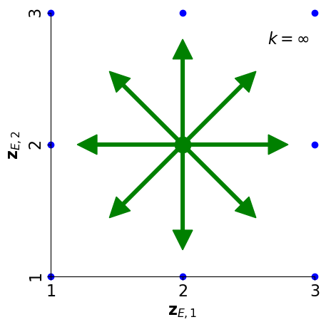
(a) All neighbors $k=\infty$

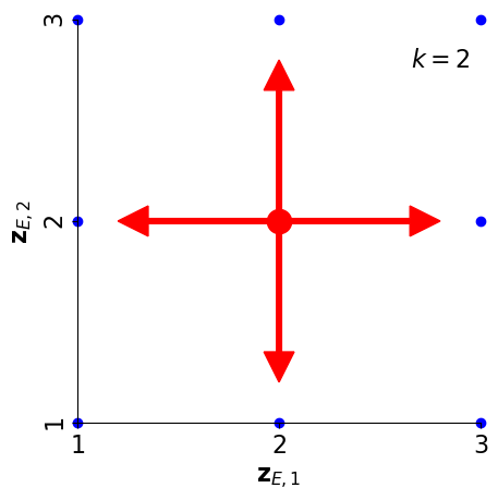
(b) Single-step neighbors $k=2$

Figure 1: Different neighborhood explorations alternatives in discrete variables lattice.

The first extension to this theory for MINLPs was introduced in [33]. This work proposed a decomposition approach for problems with ordered binary variables that were reformulated with the external variable method. The external variables created were then decoupled from the rest of the problem in an upper-level problem. Later, the D-SDA was applied to optimize the external variables in the upper-level problem where binary variables were fixed accordingly. Here, the objective function values came from the solution of NLP optimization subproblems. The main advantage of addressing superstructure optimization problems with the D-SDA is that binary variables reformulated into external variables no longer need to be evaluated at fractional solutions (e.g., a binary variable evaluated at 0.5) because evaluating points at discrete points is enough to assess discrete optimality requirements. As a result, D-SDA avoids the potential nonconvexities introduced by the continuous relaxation of MINLP superstructures, e.g., the multi-modal behavior found when optimizing the number of stages in a catalytic distillation column or the number of reactors in series [33, 35]. Also, while updating and fixing external variables successively with the D-SDA, the initialization of variables optimized in the subproblems can be monitored and updated, allowing the application of the D-SDA to highly nonlinear problems such as the optimal design of rate-based and dynamic distillation systems [36, 48].

In contrast to the IP case studied by other authors[47, 49], when considering MINLPs or GDPs, providing global optimality guarantees from a discrete convex analysis perspective is challenging since the objective function value for each discrete point corresponds to the solution of a subproblem, which is usually nonlinear. Thus, an inherent limitation of applying the D-SDA to MINLP problems is that global optimality cannot be guaranteed. Nevertheless, the D-SDA aims to find the best solution possible by choosing neighborhoods adequately. So far, the $\infty$-neighborhood has been used as a reference for local optimality in MINLP problems. One reason for this is the inclusiveness of this neighborhood, encompassing every discrete point within an infinity norm of the evaluated point, as depicted in Figure 1, instead of just positive and negative coordinates. Additionally, when applying the D-SDA with the $\infty$-neighborhood to a binary optimization problem (without reformulation), a complete enumeration over discrete variables is required. While not computationally efficient, this method offers a “brute-force” alternative for addressing small-scale discrete optimization problems.

Motivated by those previous works, in this paper, the D-SDA is extended to address more general GDP problems in the following section by directly exploring the search space of reformulated Boolean variables without the need for a (BM) or (HR) reformulations step and without the need for a linearization of the original problem as in the LOA method.

3 The Logic-based Discrete-Steepest Descent Algorithm as a Generalized Disjunctive Programming Algorithm

This section presents Logic-based D-SDA (LD-SDA) as a GDP algorithm. It begins with an explanation of the reformulation process for Boolean variables into external variables, outlining the requirements necessary for reformulation. For this, we provide a comprehensive example for demonstration. Second, the basis of the LD-SDA as a decomposition algorithm that utilizes the structure of the external variables is elucidated. The following subsection describes the different algorithms that compose the Logic-based D-SDA in the context of solving a GDP problem. The properties of LD-SDA are explained in the final subsection.

3.1 GDP Reformulations Using External Variables

Consider GDP problems where a subset of the Boolean variables in $\mathbf{Y}$ can be reformulated into a collection of integer variables referred to as external variables. Thus, $\mathbf{Y}$ in (GDP) is defined as $\mathbf{Y}=[\mathbf{Y_{R}},\mathbf{Y_{N}}]$, where $\mathbf{Y_{R}}=[\mathbf{Y_{R}}_{1},\mathbf{Y_{R}}_{2},...,\mathbf{Y_{R}}_{n_{R}}]$ contains those vectors of independent Boolean variables that can be reformulated using external variables. This means that each vector $\mathbf{Y_{R}}_{j}$ will be reformulated with one external variable, and this reformulation is applied for every $j$ in $\{1,2,...,n_{R}\}$. It is important to note that unless explicitly stated otherwise, all indices $j$ are referenced within the set $\{1,2,...,n_{R}\}$, although the explicit mention is omitted for notation simplicity. Finally, as a requisite to apply the reformulation, each vector $\mathbf{Y_{R}}_{j}$ must satisfy the following conditions:

• Requirement 1: Every Boolean variable in $\mathbf{Y_{R}}_{j}$ must be defined over a finite well-ordered set $S_{j}$ [50, p. 38]. This set may be different for each vector of variables; thus, it is indexed with $j$. In addition, variables defined over $S_{j}$ must represent ordered decisions such as finding discrete locations, selecting discrete points in time, counting the number of times a task is performed, etc. Notably, these independent Boolean variables can have indexes other than the ordered set. Also, not every Boolean variable defined over $S_{j}$ is necessarily required to be in $\mathbf{Y_{R}}_{j}$. For instance, the Boolean variables that determine the feed stage in a distillation column are defined over the set of trays, but some trays may be excluded from $\mathbf{Y_{R}}_{j}$ if needed.

• Requirement 2: Boolean variables $\mathbf{Y_{R}}_{j}$ are subject to a partitioning constraint $\texttt{Exactly}(1,\mathbf{Y_{R}}_{j})$, i.e., exactly 1 variable within $\mathbf{Y_{R}}_{j}$ is True  [51]. For example, in the case where there are only two independent Boolean variables ($\mathbf{Y_{R}}_{j}=[Y_{1},Y_{2}]$) the constraint is equivalent to $Y_{1}\veebar Y_{2}$. Note that, if the Boolean variables are transformed into binary variables, this is equivalent to a cardinality constraint $\sum_{i\in S_{j}}y_{i}=1$ [52].

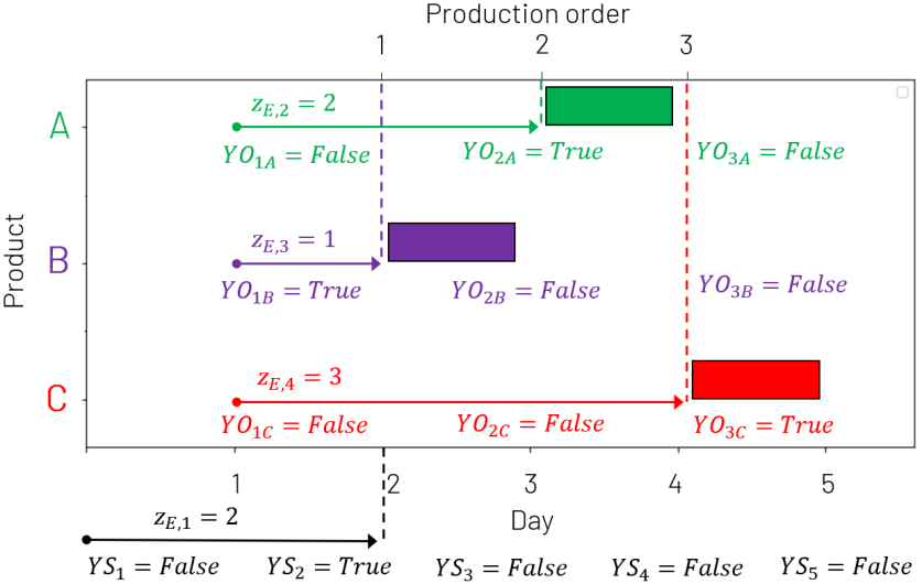
Figure 2: Reformulation of independent Boolean variables to external variables for an illustrative multi-product batch scheduling example.

To illustrate these requirements, consider the following example.

Example 1. There exists a multi-product batch reactor that produces $A$, $B$, and $C$ where the optimal starting day for each substance needs to be determined for a five-day time horizon Additionally, the order in which $A$, $B$, and $C$ are produced, subject to demand constraints, has to be established. Furthermore, it must be decided whether to perform maintenance or not before production starts. To formulate this with Boolean variables, we define $YS_{t},\forall\ t\in T=\{1,2,3,4,5\}$ to indicate the starting time; $YO_{pc},\forall\ c\in C=\{A,B,C\},\forall\ p\in P=\{1,2,3\}$ to determine the production order, and $YM$ to indicate the existence of routine maintenance. The constraints of this problem dictate that there must be only one starting day ($\texttt{Exactly}(1,\mathbf{YS}=[YS_{1},YS_{2},...,YS_{5}])$) and that each product must be produced only once ($\texttt{Exactly}(1,\mathbf{YO}_{c}=[YO_{1c},YO_{2c},YO_{3c}])\ \forall\ c\in C$). These constraints imply that variables $\mathbf{YS},\mathbf{YO}_{A},\mathbf{YO}_{B}$, and $\mathbf{YO}_{C}$ satisfy Requirement 2. Furthermore, since $T$ and $P$ are ordered sets, we conclude the aforementioned group of variables also satisfies Requirement 1. Hence, these vectors of independent Boolean variables can be grouped as $\mathbf{Y_{R}}=[\mathbf{YS},\mathbf{YO}_{A},\mathbf{YO}_{B},\mathbf{YO}_{C}]$, and reformulated with one external variable assigned to each vector in $\mathbf{Y_{R}}$. This means that ${z_{E,1}}$ is assigned to $\mathbf{YS}$, while ${z_{E,2}},{z_{E,3}}$, and ${z_{E,4}}$ are assigned to $\mathbf{YO}_{A},\mathbf{YO}_{B}$, and $\mathbf{YO}_{C}$ respectively. This reformulation is illustrated in Figure 2, where the values of reformulated Boolean variables and external variables of a potential solution are shown. In this possible solution, the operation starts on day 2, implying $YS_{2}=True\Leftrightarrow\mathbf{z}_{E,1}=2$, as shown in black at the lower horizontal axis. Analogously, the upper horizontal axis indicates the production order where the arrangement depicted is to produce $B$ first, then $A$, and finally $C$. Such production order is represented by the reformulation $YO_{1B}=True\Leftrightarrow\mathbf{z}_{E,2}=1,YO_{2A}=True\Leftrightarrow\mathbf{z}_{E,3}=2$, and $YO_{3C}=True\Leftrightarrow\mathbf{z}_{E,4}=3$. Note that the remaining Boolean variable $\mathbf{Y_{N}}=YM$ in this example does not satisfy the stated requirements. Hence, it is not reformulated. This work generalizes this external variable as discussed below.

To formally state the external variable reformulation, we consider an optimization problem in the (GDP) form. If the GDP problem satisfies Requirements 1 and 2 over the vectors of independent Boolean variables $\mathbf{Y_{R}}$, then one external variable can be assigned to each vector $\mathbf{Y_{R}}_{j}$. Requirement 1 indicates that each vector $\mathbf{Y_{R}}_{j}$ must be defined over a well-ordered set $S_{j}$. Since not every Boolean variable defined over $S_{j}$ is required to be in $\mathbf{Y_{R}}_{j}$, we declare subset $S^{\prime}_{j}\subseteq S_{j}$ to denote the ordered sets where Boolean variables $\mathbf{Y_{R}}_{j}$ are declared. We define the vectors of independent variables as $\mathbf{Y_{R}}_{j}=[Y_{Rj,S^{\prime}_{j}(1)},Y_{Rj,S^{\prime}_{j}(2)},...,Y_{Rj,S^{\prime}_{j}(\lvert S^{\prime}_{j}\rvert)}]$. This notation indicates that $Y_{Rj,S^{\prime}_{j}(a)}$ is a Boolean variable defined at position $a$ of the well-ordered set $S^{\prime}_{j}$ and included in vector $\mathbf{Y_{R}}_{j}$. Note that Boolean variables $Y_{Rj,S^{\prime}_{j}(a)}\ \forall\ a\in\{1,2,...,\lvert S^{\prime}_{j}\rvert\}$ can be defined over other sets aside from $S^{\prime}_{j}$, i.e., they may have multiple indices in the algebraic model formulation. Requirement 2 indicates that $\Omega(\mathbf{Y})=True$ in (GDP) must contain partitioning constraints of the form $\texttt{Exactly}(1,\mathbf{Y_{R}}_{j})$. Combining both requirements allows to define Boolean variables in $\mathbf{Y_{R}}$ as a function of $n_{R}$ external variables $z_{E,j}$ as:

$$Y_{Rj,S^{\prime}_{j}(a)}\iff z_{E,j}=a\quad\forall\ j\in\{1,2,...,n_{R}\},\forall\ a\in\{1,2,...,\lvert S^{\prime}_{j}\rvert\}$$ (2)

effectively expressing the external variables $z_{E,j}$ based on the values of Boolean variables $Y_{Rj,S^{\prime}_{j}(a)}$. From this reformulation, the upper and lower bounds of the external variables can be directly inferred from the sets of ordered positions $\{1,2,...,\lvert S^{\prime}_{j}\rvert\}$. These bounds are defined as:

$$1\leq z_{E,j}\leq\lvert S^{\prime}_{j}\rvert\quad\forall\ j\in\{1,2,...,n_{R}\}$$ (3)

The general external variable reformulation is given by equations (2) and (3). Now, we proceed to derive a simpler reformulation that follows from the special case when all disjunctions are defined over well-ordered sets. First, note that Requirement 2 is naturally satisfied by the disjunctions in a standard (GDP) formulation. This arises from the fact that the exclusivity requirement in disjunctions enforces constraints of the form $\texttt{Exactly}(1,\mathbf{Y}_{k}),\forall\ k\in K$, where vector $\mathbf{Y}_{k}$ contains Boolean terms $Y_{ik},\forall\ i\in D_{k}$. Consequently, if each disjunction $k$ represented an ordered decision over the well-ordered set $D_{k}$, then Requirement 1 would be directly satisfied, allowing to reformulate a standard (GDP) problem following the guidelines in equations (2) and (3) to instead obtain:

$$Y_{D_{k}(a),k}\iff z_{E,k}=a\quad\forall\ k\in K,\forall\ a\in\{1,2,...,\lvert D_{k}\rvert\}$$ (4)

$$1\leq z_{E,k}\leq\lvert D_{k}\rvert\quad\forall\ k\in K$$ (5)

respectively. In this case, there are as many external variables as disjunctions $k\in K$ in the formulation, making index $j$ interchangeable with disjunction index $k$. Similarly, ordered subsets $S^{\prime}_{j}$ correspond to disjunct sets $D_{k}$. For this reason, indexes $i$ in $Y_{ik}$ are replaced by ordered index $D_{k}(a)$ in equation (4). In practice, not every Boolean variable in the formulation fulfills the requirements to be reformulated with external variables as suggested by equation (4). In addition, ordered discrete structures may appear outside disjunctions, e.g., within $\Omega(\mathbf{Y})=True$. Therefore, the reformulation in equations (2) and (3) is more general and practical than equations (4) and (5).

Generalizing the reformulation established in earlier research, our proposed reformulation is adapted to potentially be applied over variables $\mathbf{Y_{R}}_{j}$ defined over an ordered but unevenly spaced set. For this, instead of defining external variables using elements of ordered sets as in previous works [33], we propose defining external variables with respect to the positions in ordered sets. In this case, the distance between consecutive elements in the set of positions $\{1,2,...,\lvert S^{\prime}_{j}\rvert\}$ is equal to 1. Consequently, solutions defined by isolated discrete elements will not negatively affect the LD-SDA search, whose iterations are based on a nearest-neighborhood exploration over external variables defined over positions. To illustrate this potential issue, consider, for example, an unevenly spaced set $S^{\prime}_{1}=\{0,1,2,7,10\}$, and its corresponding Boolean variables $\mathbf{Y_{R}}_{1}=[Y_{R1,0},Y_{R1,1},Y_{R1,2},Y_{R1,7},Y_{R1,10}]$, where $\texttt{Exactly}(1,\mathbf{Y_{R}}_{1})=True$. Suppose the incumbent point is $z_{E,1}=4$ (which corresponds to $Y_{R1,7}=\textit{True}$), thus its nearest neighbors are $z_{E,1}=3$ and $z_{E,1}=5$. This stems from starting at 4 and searching its immediate neighboring points i.e., 3 and 5. For those neighbors, the definitions from previous work [33] would set one of their respective Boolean variables to $True$ ($Y_{R1,3}=\textit{True}$ or $Y_{R1,5}=\textit{True}$) and the rest of Boolean variables in $\mathbf{Y_{R}}_{1}$ to False. Given that $3\notin S^{\prime}_{1}$ and $5\notin S^{\prime}_{1}$, both $z_{E,1}=3$ and $z_{E,1}=5$ would be declared as infeasible. Thus, the current incumbent $z_{E,1}=4$ would be interpreted as a local optimum, and the neighbor search will stop at this point. This problematic can be avoided using the proposed definition, where the reformulation is performed in terms of set positions. In our the example, the new definition would interpret $z_{E,1}=3$ and $z_{E,1}=5$ as positions over $\mathbf{Y_{R}}_{1}$. This means that either $Y_{R1,2}$ or $Y_{R1,10}$ would be set to True, instead of $Y_{R1,3}$ or $Y_{R1,5}$, and the discrete exploration would proceed.

3.2 GDP Decomposition Using External Variables

The reformulation presented in the previous section allows to express some of the Boolean variables in the problem in terms of the external variables as $\mathbf{Y_{R}}=\mathbf{Y_{R}}(\mathbf{z_{E}})$, where $\mathbf{z_{E}}$ is a vector of $n_{R}$ external variables. The core idea of the LD-SDA is to move these external variables to an upper-level problem (Upper) and the rest of the variables to a subproblem (Lower). This decomposition allows taking advantage of the special ordered structure of the external variables by using a Discrete-Steepest Descent Algorithm (D-SDA) in the upper level problem to explore their domain as explained in §3.3. Once an external variable configuration is determined by D-SDA, a subproblem is obtained by only considered the active disjuncts of that specific $\mathbf{z_{E}}$ configuration. The formal definition of both problems is given as:

$$\min_{\mathbf{z_{E}}} \ f_{sub}(\mathbf{z_{E}})$$ (Upper)

$$s.t. \ \mathbf{z_{E}}\in\{\underline{\mathbf{z_{E}}},\dots,\overline{\mathbf{z_{E}}}\}\subseteq\mathbb{Z}^{n_{z_{E}}} \ (\text{From Eq.}\ \eqref{eqn:ref_bounds})$$

$$s(\mathbf{{z_{E}}})=\begin{cases}f_{sub}(\mathbf{z_{E}})=&\ \min_{\mathbf{x},\mathbf{Y_{N}},\mathbf{z}}f(\mathbf{x},\mathbf{z})\\ &\ s.t.\ \mathbf{Y_{R}}=\mathbf{Y_{R}}(\mathbf{z_{E}})\ \ \ \ \ (\text{Fixed as shown in Eq.}\ \eqref{eqn:reformulation})\\ &\ \ \ \ \ \ \ \ \mathbf{g}(\mathbf{x},\mathbf{z})\leq\mathbf{0}\\ &\ \ \ \ \ \ \ \ \Omega(\mathbf{Y})=True\\ &\ \ \ \ \ \ \ \ \operatorname*{\underline{\bigvee}}_{i\in D_{k}}\left[\begin{gathered}Y_{ik}\\ \mathbf{h}_{ik}(\mathbf{x},\mathbf{z})\leq\mathbf{0}\\ \end{gathered}\right]\quad k\in K\\ &\ \ \ \ \ \ \ \ \mathbf{x}\in[\underline{\mathbf{x}},\overline{\mathbf{x}}]\subseteq\mathbb{R}^{n_{x}};\mathbf{Y}\in\{False,True\}^{n_{y}};\mathbf{z}\in\{\underline{\mathbf{z}},\dots,\overline{\mathbf{z}}\}\subseteq\mathbb{Z}^{n_{z}}\\ \end{cases}$$ (Lower)

In problem (Upper), a value for the objective function $f_{sub}(\mathbf{z_{E}})$ is obtained by the optimization of subproblem (Lower). Thus, $f_{sub}(\mathbf{z_{E}})$ is defined as the optimal objective function value found by optimizing the subproblem $s(\mathbf{z_{E}})$, obtained by fixing external variables fixed at $\mathbf{z_{E}}$. If the subproblem (Lower) is infeasible, $f_{sub}(\mathbf{z_{E}})$ is set to as infinity by convention. Notably, the subproblems are reduced formulation given that they only consider the relevant constraints for the relevant external variable configuration $\mathbf{z_{E}}$.

A novel feature of the LD-SDA is its ability to handle various types of subproblems, extending previous versions [33], which solely supported NLP subproblems. In its most general form, the lower-layer problem (Lower) is a (GDP) with continuous ($\mathbf{x}$), discrete ($\mathbf{z}$) and non-reformulated Boolean ($\mathbf{Y_{N}}$) variables. Consider the scenario where every Boolean variable can be reformulated (e.g., as shown in equations (4) and (5)) or every non-reformulated variable $\mathbf{Y_{N}}$ is equivalently expressed in terms of $\mathbf{Y_{R}}$. Note that the later situation may occur if all Boolean variables $\mathbf{Y_{N}}$ are determined within the subproblem upon fixing $\mathbf{Y_{R}}$, implying that logic constraints $\Omega(\mathbf{Y})=True$ establish $\mathbf{Y_{N}}$ as functions of $\mathbf{Y_{R}}$. In such a scenario, the resulting subproblem becomes an (MINLP) with continuous ($\mathbf{x}$) and discrete variables ($\mathbf{z}$), or an NLP if there are no discrete variables ($\mathbf{z}$) in the formulation. In the following subsection, we introduce the LD-SDA as a decomposition algorithm that leverages the external variable reformulation and bi-level structure depicted so far.

3.3 Logic-based Discrete-Steepest Descent Algorithm

The Logic-based Discrete-Steepest Descent Algorithm (LD-SDA), as described in Algorithm 1, solves a series of subproblems (Lower) until a stopping criterion is satisfied. The LD-SDA can only start once the external variable reformulation of the problem has been performed. The external variables $\mathbf{{z_{E}}}$ are handled in an upper optimization layer where the algorithm is performed. To initialize, this method requires an initial fixed value of external variables $\mathbf{{z_{E,0}}}$, the value of the variables of its corresponding feasible solution ($\mathbf{{x}_{0}},\mathbf{{Y}_{0}},\mathbf{{z}_{0}}$), and its respective objective function value $f_{sub}(\mathbf{{z_{E,0}}})$. Finding a starting feasible solution is beyond the scope of this work; however, it would be enough to have $\mathbf{{z_{E,0}}}$ and solve the subproblem $s(\mathbf{{z_{E,0}}})$ to find the rest of the required initial solution. Note that problem-specific initialization strategies have been suggested in the literature, e.g., see [48].

The LD-SDA explores a neighborhood within the external variable domain; hence, the user must to determine the type of neighborhood $k$ that will be studied. In this paper, we only consider $k\in\{2,\infty\}$ as shown in Figure 1; nevertheless, other types of discrete neighborhoods can be considered [34]. Once $k$ has been selected, the neighborhood $N_{k}$ of a given point $\mathbf{{z_{E}}}$ is defined as $N_{k}(\mathbf{{z}_{E}})=\{\mathbf{\alpha}\in\mathbb{Z}^{n_{z_{E}}}:\;\lVert\mathbf{\alpha}-\mathbf{{z}_{E}}\rVert_{k}\leq 1\}$. Similarly, the set of distances $\Delta_{k}$ from the point $\mathbf{{z_{E}}}$ to each neighbor $\mathbf{\alpha}$ is be calculated as $\Delta_{k}(\mathbf{{z}_{E}})=\{\mathbf{d}:\;\mathbf{\alpha}-\mathbf{{z}_{E}}=\mathbf{d},\forall\ \mathbf{\alpha}\in N_{k}(\mathbf{{z}_{E}})\}$.

The next step is to perform Neighbor Search (see Algorithm 2), which consists of a local search within the defined neighborhood. Essentially, this algorithm solves $s(\mathbf{\alpha})\;\forall\;\mathbf{\alpha}\in N_{k}(\mathbf{{z}_{E}})$ and compares the solutions found with the best incumbent solution $f_{sub}(\mathbf{z_{E}})$. If, in a minimization problem, $f_{sub}(\mathbf{z_{E}})\leq f_{sub}(\mathbf{\alpha})\;\forall\;\mathbf{\alpha}\in N_{k}(\mathbf{{z}_{E}})$ then, the current solution in $\mathbf{{z}_{E}}$ is a discrete local minimum (i-local or s-local depending on the value of $k$); otherwise, the steepest descent direction $\mathbf{d^{*}}=\mathbf{\alpha^{*}}-\mathbf{{z}_{E}}$ is computed, the algorithm moves to the best neighbor by letting $\mathbf{{z}_{E}}=\mathbf{\alpha^{*}}$ and performs a Line Search in direction $\mathbf{d^{*}}$. Note that for a neighbor to be considered the best neighbor $\mathbf{\alpha^{*}}$, it must have a feasible subproblem and a strictly better objective than both the incumbent solution and its corresponding neighborhood.

The Line Search (see Algorithm 3) determines a point in the direction of steepest descent $\mathbf{\beta}=\mathbf{{z}_{E}}+\mathbf{d^{*}}$ and evaluates it. If the subproblem $s(\mathbf{\beta})$ is feasible and $f_{sub}(\mathbf{\beta})<f_{sub}(\mathbf{z_{E}})$ then, let $\mathbf{{z}_{E}}=\mathbf{\beta}$ and perform the Line Search again until the search is unable to find a better feasible solution in direction $\mathbf{d^{*}}$. Once this occurs, the general algorithm should return to calculate $N_{k}(\mathbf{{z}_{E}})$ and $\Delta_{k}(\mathbf{{z}_{E}})$ to perform the Neighbor Search again in a new iteration.

The LD-SDA will terminate once the Neighbor Search is unable to find a neighbor $\mathbf{\alpha}$ with a feasible subproblem $s(\mathbf{\alpha})$ that strictly improves the incumbent solution as $f_{sub}(\mathbf{\alpha})<f_{sub}(\mathbf{z_{E}})\;\forall\;\mathbf{\alpha}\in N_{k}(\mathbf{{z}_{E}})$. In that case, the point is considered a discrete i-local or s-local minimum, and the algorithm will return the values of both variables ($\mathbf{{x}},\mathbf{{Y}},\mathbf{{z}},\mathbf{{z_{E}}}$) and the objective function $f_{sub}^{*}$ of the solution found. The stopping criterion employed indicates that the current point has the best objective function amongst its immediate discrete neighborhood mapping [34]. In rigorous terms, the integrally local optimality condition can only be guaranteed after an $N_{\infty}$ exploration given that this is the neighborhood that considers the entire set of immediate neighbors (i-local optimality). Therefore, when using neighborhood $N_{2}$, it is up to the user to choose if the final solution $\mathbf{\hat{z_{E}}}$ is to be certified as integrally local by checking its $N_{\infty}(\mathbf{\hat{z_{E}}})$ neighborhood.

Figure 3 illustrates and explains the LD-SDA executed in its entirety on a 6$\times$6 lattice of two external variables. For this example, the $\infty$-neighborhood is utilized and two different Neighbor Searches are required. Furthermore, a detailed pseudo-code for the LD-SDA is presented below. Additional efficiency improvements and other implementation details are presented in §4.

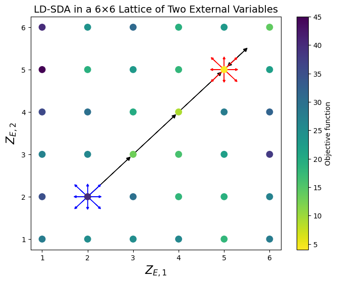
Figure 3: LD-SDA with $k=\infty$. First, the algorithm is initialized in $[2,2]$. Neighbor Search in the neighborhood $N_{\infty}({[2,2]})$ (represented with blue arrows) finds the best neighbor is ${[3,3]}$; hence, the steepest descent direction $\mathbf{d^{*}}$ is ${[1,1]}$. Then, Line Search (represented with black arrows) is performed up to point ${[5,5]}$ and stopped there because $f_{sub}({[5,5]})<f_{sub}({[5,5]}+\mathbf{d^{*}})$. A second Neighbor Search in $N_{\infty}({[5,5]})$ is performed (represented in red arrows) and concludes that point ${[5,5]}$ is integrally local; therefore, the algorithm terminates.

1

Input: $k\in\{2,\infty\}$ ; An external variable feasible solution $\mathbf{{z}_{E,0}}$

Data: Variable values associated with feasible solution $\mathbf{{x}_{0}},\mathbf{{Y}_{0}},\mathbf{{z}_{0}}$

/* Initialize */

2 Set $\mathbf{{x}}\leftarrow\mathbf{{x}_{0}};\;\;\mathbf{Y}\leftarrow\mathbf{{Y}_{0}};\;\;\mathbf{z}\leftarrow\mathbf{{z}_{0}};\;\;\mathbf{z_{E}}\leftarrow\mathbf{{z}_{E,0}}$

3 Solve subproblem: $f_{sub}^{*}\leftarrow f_{sub}(\mathbf{z_{E}})$

4 Set neighborSearching $\leftarrow True$

Generate initialization: $\gamma_{init}\leftarrow\{\mathbf{{x}},\mathbf{{Y}},\mathbf{{z}},\mathbf{{z_{E}}}\}$

  // Optional

Initialize set of explored point in lattice as $G\leftarrow\{\mathbf{{z}_{E}}\}$

  // Optional

/* This cycle performs Neighbor Search either when the algorithm starts (after initialization) or when Line Search does not improve the incumbent solution */

5 while neighborSearching is $True$ do

       /* Find the current neighborhood $N_{k}(\mathbf{{z}_{E}})$ and directions $\Delta_{k}(\mathbf{{z}_{E}})$ to execute Neighbor Search */

6       Compute $N_{k}(\mathbf{{z}_{E}})=\{\mathbf{\alpha}\in\mathbb{Z}^{n_{z_{E}}}:\;\lVert\mathbf{\alpha}-\mathbf{{z}_{E}}\rVert_{k}\leq 1\}$

7       Compute $\Delta_{k}(\mathbf{{z}_{E}})=\{\mathbf{d}:\;\mathbf{\alpha}-\mathbf{{z}_{E}}=\mathbf{d},\forall\ \mathbf{\alpha}\in N_{k}(\mathbf{{z}_{E}})\}$

8      

      /* Perform the Neighbor Search by evaluating an comparing every $f_{sub}(\mathbf{\alpha})$ */

9      

10      $f_{sub}^{*}\;;\;\mathbf{{z_{E}}}\;;\;\mathbf{{d^{*}}}\;;\;\texttt{improvedDuringNS}\;;\;\gamma_{init}\leftarrow$ Neighbor Search($f_{sub}^{*},\mathbf{{z}_{E}},N_{k}(\mathbf{{z}_{E}}),\Delta_{k}(\mathbf{{z}_{E}})$)

      /* Check for improvement during Neighbor Search */

11      

12      if improvedDuringNS is $True$ then

             /* If so, perform Line Search in direction $\mathbf{d^{*}}$ until the incumbent does not improve */

13             Set lineSearching $\leftarrow True$

14             while lineSearching is $True$ do

15                   $f_{sub}^{*}\;;\;\mathbf{{z_{E}}}\;;\;\texttt{improvedDuringLS}\;;\;\gamma_{init}\leftarrow$ Line Search($f_{sub}^{*},\mathbf{{z}_{E}},\mathbf{d^{*}}$)

                   /* Check if the current solution was not improved during Line Search */

16                   if improvedDuringLS is $False$ then

                         /* If so, stop Line Search */

17                         Set lineSearching $\leftarrow False$

18                        

19                  

20            

21      else

             /* If not, stop Neighbor Search to terminate the algorithm and return the solution */

22             Set neighborSearching $\leftarrow False$

23      

Output: $f_{sub}^{*}\;;\;\mathbf{{x}}\;;\;\mathbf{{Y}}\;;\;\mathbf{{z}}\;;\;\mathbf{{z_{E}}}$

24

Algorithm 1 Logic-based Discrete-Steepest Descent Algorithm (LD-SDA)

3.3.1 Neighbor Search and Line Search

In this subsection we present detailed pseudo-codes and intuitions on implementing the Neighbor Search and the Line Search algorithms as presented in Algorithm 2 and Algorithm 3, respectively.

In a general sense, the Neighbor Search algorithm is a local search around the immediate neighborhood of discrete variables from a starting point $\mathbf{{z}_{E}}$. Therefore, the neighborhood $N_{k}(\mathbf{{z}_{E}})$ and the set of distances corresponding to each neighbor $\Delta_{k}(\mathbf{{z}_{E}})$ must be computed before starting the exploration. This algorithm solves the subproblems $s(\mathbf{\alpha})\;\forall\ \mathbf{\alpha}\in N_{k}(\mathbf{{z}_{E}})$ and compares their objective function; if feasible, with the best incumbent solution found by Neighbor Search $f_{sub}^{NS}$ so far.

Neighbor Search determines whether a new neighbor $\mathbf{\alpha}$ improves the current solution $\mathbf{z_{E}}$ based on two criteria, which can be evaluated in relative or absolute terms. The first criterion employs a strict less ($<$) comparison and is utilized when no neighbor has yet improved upon the current solution. This ensures the algorithm does not transition to a neighbor with an identical objective, thereby preventing cycling between points with identical objective functions. Further discussion on the non-cycling properties of the LD-SDA is provided in §3.4. The second criterion, employing a less-than-or-equal-to ($\leq$) comparison, becomes active once a single neighbor $\mathbf{\alpha}$ improves upon the incumbent solution. This enables the algorithm to consider multiple $\mathbf{\alpha}$’s with the same objective. Consequently, if more than one neighbor shares the best current solution, a maximum Euclidean distance lexicographic heuristic may be employed as a tie-break criterion. This heuristic calculates the Euclidean distance as $\texttt{dist}=\lVert\mathbf{\alpha}-\mathbf{{z}_{E}}\rVert_{2}\;\forall\ \mathbf{\alpha}\in N_{k}(\mathbf{{z}_{E}})$, favoring the first-found "most diagonal" routes. Such routes, absent in $N_{2}$ neighborhoods, have proven effective in previous versions of the D-SDA[33, 35, 36].

1

Input: $f_{sub}^{*}\;;\;\mathbf{{z}_{E}}\;;\;N_{k}(\mathbf{{z}_{E}})\;;\;\Delta_{k}(\mathbf{{z}_{E}})$

2

/* Initialize */

3

4Relative tolerance $\epsilon$

5 Set improvedDuringNS $\leftarrow False;\;\;\mathbf{d^{*}}\leftarrow\mathbf{0};\;\;f_{sub}^{NS}\leftarrow\infty$

Set $\texttt{dist}^{*}\leftarrow 0$

  // Optional

6

7for every $\mathbf{\alpha_{i}}\in N_{k}(\mathbf{{z}_{E}})$  do

       /* Optional: Check if the neighbor was already evaluated in a previous iteration */

8       if $\mathbf{\alpha_{i}}\in G$  then

9             Go to line 4 with $\mathbf{\alpha_{i+1}}$

10      else

11            Append $\mathbf{\alpha_{i}}$ to $G$

12      

      /* Optional: Check if the neighbor is within external variable domain */

13       if $\mathbf{\alpha_{i}}\notin\mathbf{Z_{E}}=\{\mathbf{1},\dots,\overline{\mathbf{z_{E}}}\}$ then

14             Go to line 4 with $\mathbf{\alpha_{i+1}}$

15      

      /* Create fixed subproblem */

16      

17      Create subproblem and fix with external variables $s(\mathbf{\alpha_{i}})$

       Initialize $s(\mathbf{\alpha_{i}})$ using $\gamma_{init}$

        // Optional

       /* Optional: Check feasibility of fixed external variables in $s(\mathbf{\alpha_{i}})$ with FBBT */

18      

19      if FBBT of $s(\mathbf{\alpha_{i}})$ detects infeasibility then

20             Go to line 4 with $\mathbf{\alpha_{i+1}}$

      /* Solve subproblem */

21       Solve $s(\mathbf{\alpha_{i}})$

22      if $s(\mathbf{\alpha_{i}})$ is feasible then

23             Set $f_{sub}^{NS}\leftarrow f_{sub}(\mathbf{\alpha_{i}})$

24            

            Set $\texttt{dist}_{i}\leftarrow\lVert\mathbf{\alpha_{i}}-\mathbf{{z}_{E}}\rVert_{2}$

              // Optional

25            

            /* Check if the algorithm has already improved the starting solution to choose the corresponding minimum improvement criterion */

26            

27            if improvedDuringNS is $False$ then

28                  

                  /* Check if minimum improvement criterion is satisfied */

29                  

30                  if $f_{sub}^{NS}<f_{sub}^{*}$ or $(f_{sub}^{*}-f_{sub}^{NS})/(\lvert f_{sub}^{*}\rvert+10^{-10})>\epsilon$ then

                         /* Update with new best solution */

31                         Set $f_{sub}^{*}\leftarrow f_{sub}^{NS}$; $\mathbf{d^{*}}\leftarrow\Delta_{k}(\mathbf{{z}_{E}})_{\mathbf{i}}$; $\mathbf{{z}_{E}}\leftarrow\mathbf{\alpha_{i}}$

32                         Set $\texttt{improvedDuringNS}\leftarrow True$

                         Set $\texttt{dist}^{*}\leftarrow\texttt{dist}_{i}$

                          // Optional

33                        

                        Generate initialization: $\gamma_{init}\leftarrow\{\mathbf{{x}},\mathbf{{Y}},\mathbf{{z}},\mathbf{{z_{E}}}\}$

                          // Optional

34                        

35                  

36            else

                   /* Check if minimum improvement criterion is satisfied. There is an additional condition that implements the maximum Euclidean distance heuristic */

37                  

38                  if $(f_{sub}^{NS}\leq f_{sub}^{*}$ or $(f_{sub}^{*}-f_{sub}^{NS})/(\lvert f_{sub}^{*}\rvert+10^{-10})\geq\epsilon)$ and $\texttt{dist}_{i}\geq\texttt{dist}^{*}$ then

                         /* Update with new best solution */

39                         Set $f_{sub}^{*}\leftarrow f_{sub}^{NS}$; $\mathbf{d^{*}}\leftarrow\Delta_{k}(\mathbf{{z}_{E}})_{\mathbf{i}}$; $\mathbf{{z}_{E}}\leftarrow\mathbf{\alpha_{i}}$

40                         Set $\texttt{improvedDuringNS}\leftarrow True$

                         Set $\texttt{dist}^{*}\leftarrow\texttt{dist}_{i}$

                          // Optional

41                        

                        Generate initialization: $\gamma_{init}\leftarrow\{\mathbf{{x}},\mathbf{{Y}},\mathbf{{z}},\mathbf{{z_{E}}}\}$

                          // Optional

42                        

43                  

44            

45      

Output: $f_{sub}^{*}\;;\;\mathbf{{z_{E}}}\;;\;\mathbf{{d^{*}}}\;;\;\texttt{improvedDuringNS}\;;\;\gamma_{init}$

Algorithm 2 Neighbor Search

The Line Search algorithm is a search in the steepest descent direction, determined by the direction of the best neighbor $\mathbf{d^{*}}=\mathbf{\alpha^{*}}-\mathbf{z_{E}}$. This approach generates a point in the steepest descent direction $\mathbf{\beta}=\mathbf{z_{E}}+\mathbf{d^{*}}$ and solves the optimization subproblem $s(\mathbf{\beta})$ to obtain $f_{sub}^{LS}$. The algorithm moves to the point $\mathbf{\beta}$ if and only if, $s(\mathbf{\beta})$ is feasible and $f_{sub}^{LS}<f_{sub}^{*}$, adhering to the strict less-than ($<$) improvement criterion. This criterion prevents revisiting previous points, thereby accelerating and ensuring convergence. Again, more insights into the convergence properties of the LD-SDA are stated in §3.4. The Line Search process continues until there is no feasible point in the direction $\mathbf{d^{*}}$ that improves upon the incumbent solution.

1

Input: $f_{sub}^{*}\;;\;\mathbf{{z}_{E}}\;;\;\mathbf{d^{*}}$

2

/* Initialize */

3

4Relative tolerance $\epsilon$

5 Set improvedDuringLS $\leftarrow False;\;\;\mathbf{\beta}\leftarrow\mathbf{{z}_{E}}+\mathbf{d^{*}};\;\;f_{sub}^{LS}\leftarrow\infty$

/* Optional: Check if the moved point $\beta$ was already evaluated in a previous iteration */

6 if $\mathbf{\beta}\in G$ then

7       Terminate algorithm

8else

9      Append $\mathbf{\beta}$ to $G$

10

/* Optional: Check if the moved point is within the external variable domain */

11 if $\mathbf{\beta}\notin\mathbf{Z_{E}}=\{\mathbf{1},\dots,\overline{\mathbf{z_{E}}}\}$ then

12       Terminate algorithm

13

/* Create fixed subproblem */

14

15Create subproblem and fix with external variables $s(\mathbf{\beta})$

Initialize $s(\mathbf{\beta})$ using $\gamma_{init}$

  // Optional

/* Optional: Check feasibility of fixed external variables in $s(\mathbf{\beta})$ with FBBT */

16

17if FBBT of $s(\mathbf{\beta})$ detects infeasibility then

18       Terminate algorithm

/* Solve subproblem */

19 Solve $s(\mathbf{\beta})$

20if $s(\mathbf{\beta})$ is feasible then

21       Set $f_{sub}^{LS}\leftarrow f_{sub}(\mathbf{\beta})$

22      

      /* Check if minimum improvement criterion is satisfied */

23      

24      if $f_{sub}^{LS}<f_{sub}^{*}$ or $(f_{sub}^{*}-f_{sub}^{LS})/(\lvert f_{sub}^{*}\rvert+10^{-10})>\epsilon$ then

             /* Update with new best solution */

25             Set $f_{sub}^{*}\leftarrow f_{sub}^{LS}$; $\mathbf{{z}_{E}}\leftarrow\mathbf{\beta}$

26             Set $\texttt{improvedDuringLS}\leftarrow True$

27            

            Generate initialization: $\gamma_{init}\leftarrow\{\mathbf{{x}},\mathbf{{Y}},\mathbf{{z}},\mathbf{{z_{E}}}\}$

              // Optional

28            

29      

30

Output: $f_{sub}^{*}\;;\;\mathbf{{z_{E}}}\;;\;\texttt{improvedDuringLS}\;;\;\gamma_{init}$

Algorithm 3 Line Search

3.4 Logic-based Discrete-Steepest Descent Algorithm Properties

The LD-SDA algorithm is guaranteed not to cycle, i.e., it will not re-evaluate the same solution candidates when searching for the optimal solution. This is avoiding revisiting previously solved subproblems, and it can be accomplished carefully evaluating when to move to a next incumbent. In both Neighbor Search (Algorithm 2) and Line Search (Algorithm 3), the algorithms ensure improvement in the solution of the next discrete point by following to a minimum improvement criterion. As established in §3.3.1, this criterion is satisfied if and only if a strict ($<$) improvement is obtained. Consequently, if this criterion is met, the algorithms update the incumbent with the new best solution discovered during the searches, ensuring only strictly better solutions are considered. It is important to note that this criterion excludes points with the same objective value as the incumbent, thereby preventing cycling between points with identical objectives. By avoiding revisiting points in the lattice, the algorithms prevent the steepest descent from retracing its steps in either the Neighbor or Line Search steps. This verification not only guarantees convergence to a discrete local minimum but also saves computational time, as the algorithm never re-evaluates the same point.

The primary advantage of the LD-SDA over previous iterations of the D-SDA lies in its utilization of the structure of ordered Boolean variables for external variable reformulation, as opposed to ordered binary variables. In the LD-SDA, the solution to the upper-level problem is the same as the one used in the D-SDA, involving a series of Neighbor and Line searches over the external variable lattice. However, the key distinction is that each lattice point in the LD-SDA upper-level problem corresponds to a reduced space GDP or (MI)NLP, obtained by fixing Booleans and thereby disjunctions (see §3.2). This approach results in a reduced subproblem that considers only relevant constraints, effectively circumventing zero-flow issues and improving numerical stability and computational tractability. In contrast, previous versions of the D-SDA fixed binary variables to obtain NLP subproblems, which could potentially contain irrelevant constraints with respect to the current configuration of the Boolean variables yielding and ill-posed behavior. Furthermore, additional algorithmic improvements with respect to previous versions of the D-SDA were added to the LD-SDA as discussed in §4.

3.5 Equivalence to Other Generalized Disjunctive Programming Algorithms

While LD-SDA exhibits different features compared to other GDP algorithms, certain aspects of it remain equivalent to them. Notably, akin to other logic-based approaches, LD-SDA addresses (MI)NLP subproblems containing only the constraints of active disjunctions, thereby excluding irrelevant nonlinear constraints. Each method employs a mechanism for selecting the subsequent (MI)NLP subproblem, typically based on a search procedure. In LOA, this mechanism involves solving a MILP problem subsequent to reformulating Problem (Main l-GDP). On the other hand, LBB determines a sequence of branched disjunctions for each layer $l$, $KB_{l}$, based on a predetermined rule known as branching rule. In contrast, LD-SDA utilizes Neighbor and Line Search algorithms to make this decision, solving Problem (Upper) locally.

The LD-SDA employs an external variable reformulation to map Boolean variables into a lower-dimensional representation of discrete variables. While LD-SDA solves the upper-level problem through steepest descent optimization, this problem essentially constitutes a discrete optimization problem without access to the functional form of the objective. Hence, in principle, this problem could be addressed using black-box optimization methods. Moving from one point to another within the discrete external variable lattice involves changing the configuration of Boolean variables in the original problem, often modifying multiple Boolean variables simultaneously. Consequently, the LD-SDA can be viewed as a variant of LBB, where Neighbor and Line Searches act as sophisticated branching rules for obtaining Boolean configurations to fix and evaluate. Additionally, improvements to this problem could be achieved by leveraging information from the original GDP problem. For instance, linear approximations of the nonlinear constraints of the GDP could be provided, although this would necessitate employing a MILP solver. By constructing such linearizations around the solutions of the subproblem (Lower), one could recover Problem (Main l-GDP) from LOA.

4 Implementation Details

The LD-SDA, as a solution method for GDP, was implemented in Python using Pyomo [40] as an open-source algebraic modeling language. Pyomo.GDP [41] was used to implement the GDP models and use their data structures for the LD-SDA. The code implementation allows the automatic reformulation of the Boolean variables in the GDP into external variables and provides an efficient implementation of the search algorithms over the lattice of external variables.

4.1 Automatic Reformulation

In contrast to previous works for MINLP models [33], the reformulation in (2) and (3) provides a generalized framework that is automated in the Python implementation developed in this work. Minimal user input is required for the reformulation process, with only the Boolean variables in $\mathbf{Y}$ defined over ordered sets $S_{j},\forall\ j\in\{1,2,...,n_{R}\}$ needing specification. This reformulation allows fixing Boolean variables based on the values of external variables. Moreover, additional Boolean variables can be fixed based on the values of the external variables, as users can specify those Boolean variables in $\mathbf{Y_{N}}$ that are equivalent to expressions of the independent Boolean variables $\mathbf{Y_{R}}$ through logic constraints $\Omega(\mathbf{Y})=True$.

4.2 Algorithmic Efficiency Improvements

This section presents the four major efficiency improvements are included in the algorithm and are indicated throughout the pseudo-codes in §3.3 as Optional.

4.2.1 Globally Visited Set Verification

Due to the alternating dynamic between Line Search and Neighbor Search, the LD-SDA often queues discrete points that were previously visited and evaluated. An example of this issue can be observed in Figure 3 where the second Neighbor Search in $N_{\infty}({[5,5]})$, depicted in red, visits points ${[4,4]}$ and ${[6,6]}$ that had already been evaluated during Line Search (shown in black). The number of reevaluated points depends on how close to the Neighbor Search the Line Search stops, increasing proportionally with the number of external variables.

Although re-evaluating points does not affect the convergence of the algorithm as discussed in §3.4, it results in unnecessary additional computation that can be avoided. This redundant evaluation existed in the previous versions of the D-SDA [33, 35, 36] and can be rectified by maintaining a globally visited set $G$ (line 1 of Algorithm 1). Now, before solving the optimization model for a particular point $\mathbf{\alpha}$ (lines 2 to 2 of Algorithm 2) or $\mathbf{\beta}$ (lines 3 to 3 of Algorithm 3), the algorithm verifies if the point has already been visited. If so, the algorithm disregards that point and either proceeds to the next $\mathbf{\alpha}$ in the Neighbor Search or terminates the Line Search algorithm.

4.2.2 External Variable Domain Verification

All external variables must be defined over a constrained box $\mathbf{Z_{E}}=\{\mathbf{1},\dots,\overline{\mathbf{z_{E}}}\}$ (as shown in Eq. (3)) that depends on the problem. For superstructure problems, this domain is bounded by the size of the superstructure, such as the number of potential trays in a distillation column or the maximum number of available parallel units in a process. Similarly, for scheduling problems, the external variable domain can be given by the scheduling horizon.

External variables with non-positive values or exceeding the potential size of the problem, resulting in a lack of physical sense, should not be considered in the explorations. To prevent unnecessary presolve computations, the algorithm verifies if the incumbent point ($\mathbf{\alpha}$ or $\mathbf{\beta}$) belongs to $\mathbf{Z_{E}}$ before solving the optimization model, effectively avoiding consideration of infeasible subproblems. If during Neighbor Search $\mathbf{\alpha}\notin\mathbf{Z_{E}}$, the neighbor $\mathbf{\alpha}$ can be ignored and the algorithm proceeds to explore the next neighbor. Similarly, if $\mathbf{\beta}\notin\mathbf{Z_{E}}$ while performing the Line Search, the algorithm should return to $\mathbf{z_{E}}=\mathbf{\beta}-\mathbf{d^{*}}$ and terminate. Returning to the example shown in Figure 3, note that, for instance, $N_{\infty}([1,6])=\{[2,6],[2,5],[1,5]\}$ given that points $\{[1,7],[2,7],[0,5],[0,6],[0,7]\}$ can be automatically discarded and considered infeasible since $\mathbf{z_{E,1}},\mathbf{z_{E,2}}\in\{1,2,...,6\}$.

4.2.3 Fixed External Variable Feasibility Verification via FBBT

The existence of external variables $\mathbf{z_{E}}$ within their respective bounds does not ensure feasibility in the subproblem $s(\mathbf{z_{E}})$. While external variables can encode a physical interpretation of the problem by representing specific positions within a well-ordered set, constraints concerning the rest of the problem must align with spatial information to achieve a feasible subproblem. For instance, consider the distillation column (discussed in §5.2) that has two external variables: one determining the reflux position $z_{E,R}$ and another determining the boil-up position $z_{E,B}$. The problem has an implicit positional constraint $z_{E,B}<z_{E,R}$, indicating that the boil-up stage must be above the reflux stage when counting trays from top to bottom. Throughout the algorithm, this type of discrete positional constraint, which relates external variables, is frequently violated when a particular $\mathbf{z_{E}}$ is fixed in a subproblem $s(\mathbf{z_{E}})$. This violation arises because these constraints are specified in the original GDP model in terms of Boolean variables. Consequently, after the external variable reformulation, fixed points in the discrete lattice may overlook the original logical constraints.

In previous works [33, 35, 36], users were tasked with manually re-specifying these constraints in the domain of external variables. However, this work aims to automate this requirement. Instead of solving infeasible models that consume computation time and may generate errors terminating the algorithm, we used Feasibility-based Bound Tightening (FBBT), which is available in Pyomo. FBBT rapidly verifies feasibility over the fixed Boolean constraints, enabling the algorithm to identify subproblem infeasibility without executing a more resource-intensive MINLP or GDP presolve algorithm. Now, if FBBT determines that a subproblem $s(\mathbf{z_{E}})$ is infeasible, the point $\mathbf{z_{E}}$ can be instantly disregarded.

4.2.4 Re-initialization Scheme

The LD-SDA method incorporates an efficiency improvement that involves reinitializing from the best solution $\gamma_{init}=\{\mathbf{{x}},\mathbf{{Y}},\mathbf{{z}},\mathbf{{z_{E}}}\}$. Effective model initialization is crucial for achieving faster convergence, particularly as problems increase in size and complexity. Initiating a discrete point with the solution of a neighboring point is intuitively reasonable. Since points in the external variable lattice are derived from Boolean configurations following ordered sets, adjacent points are expected to yield very similar subproblems (e.g., adding an extra tray in a distillation column or starting a process one time step later). Therefore, initializing from an adjacent neighbor can offer an advantage of discrete-steepest descent optimization over black-box methods that search the lattice.

During Neighbor Search with $\mathbf{\alpha}\in N_{k}(\mathbf{{z}_{E}})$, all subproblems are initialized using the solved variable values from the best incumbent solution $s(\mathbf{z_{E}})$. Similarly, in Line Search each subproblem from the moved point $s(\mathbf{\beta})$ is initialized with the variable values of the best incumbent solution $s(\mathbf{z_{E}}=\mathbf{\beta}-\mathbf{d^{*}})$. This reinitialization methodology proved very efficient when integrated into the MINLP D-SDA in the rigorous design of a catalytic distillation column using a rate-based model [36].

5 Results

The LD-SDA is implemented as an open-source code using Python. The case studies, such as reactors, chemical batch processing, and binary distillation column design, are modeled using Python 3.7.7 and Pyomo 5.7.3 [40]. The catalytic distillation column design case study was modeled using GAMS 36.2.0. All the solvers used for the subproblems are available in that version of GAMS and were solved using a Linux cluster with 48 AMD EPYC 7643 2.3GHz CPU processors and 1.0 TB RAM. All the codes are available at https://github.com/SECQUOIA/dsda-gdp. The solvers used for the MINLP optimization are BARON [53], SCIP [54], ANTIGONE [55], DICOPT [56], SBB [57], and KNITRO [58]. KNITRO, BARON, and CONOPT [59] are used to solve the NLP problems. The GDP reformulations and algorithms are implemented in GDPOpt [41].

5.1 Series of Continuously Stirred Tank Reactors (CSTRs)

Consider a reactor network adapted from  [33], consisting of a superstructure of $N_{T}$ reactors in series (depicted in Figure 4), where $N_{T}$ represents the total number of potential reactors to install. The objective is to minimize the sum of reactor volumes. The network involves an autocatalytic reaction $A+B\rightarrow 2B$ with a first-order reaction rate, along with mass balances and reaction equations for each reactor. Logical constraints define the recycle flow location and the number of CSTRs in series to install. All installed reactors must have the same volume and a single recycle stream can feed any of them. Interestingly, as the number of reactors increases and the recycle is placed in the first reactor, the system approximates to a plug-flow reactor, minimizing the total volume and providing an asymptotic analytical solution. We investigate this feature by varying the number of potential reactors $N_{T}$. For a detailed formulation of the reactor series superstructure, refer to Appendix A.1.

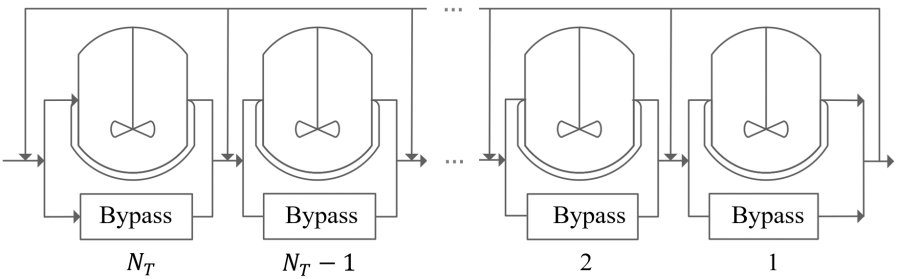
Figure 4: Reactor series superstructure with $N_{T}$ potential reactors

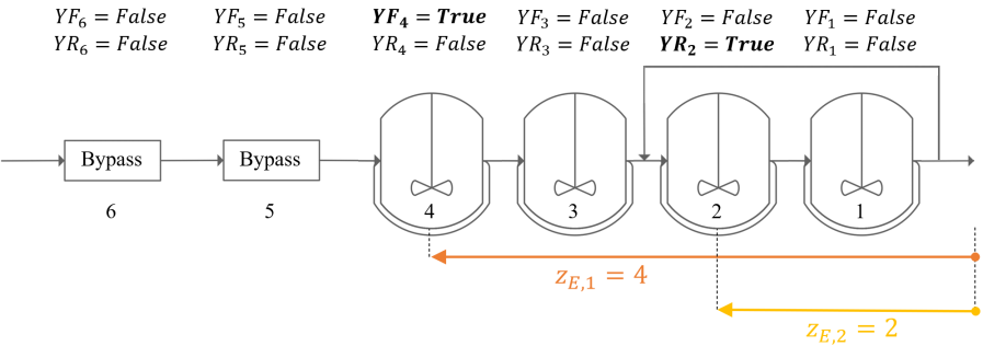
Figure 5: Reformulation for an illustrative feasible configuration of the reactor series with $N_{T}=6$.

The external variables $\mathbf{z_{E}}=[z_{E,1}:\text{No. of reactors (related with }YF),z_{E,2}:\text{Recycle position (related with }YR)]$ as shown in Figure 5 are the result of a complete reformulation of logic variables into external integer variables (detailed in Appendix B.1). This figure shows the binaries associated with the values of the ordered Boolean variables and their corresponding external variable mapping for an illustrative feasible solution, effectively indicating the reformulation $YF_{4}=True\Leftrightarrow{z}_{E,1}=4$ and $YR_{2}=True\Leftrightarrow{z}_{E,2}=2$.

We analyze the paths and solutions generated by the LD-SDA under varying neighborhood selections, as depicted in Figure 6. Given $N_{T}$ series of potential reactors, the problem is initialized with one reactor and its recycle flow. This initialization is represented in the integer variables lattice as a single reactor with a reflux position immediately behind it ($\mathbf{z_{E}}=[1,1]$). For LD-SDA employing a $k=2$ neighborhood search, the algorithm identifies $[2,1]$ is locally optimal and proceeds with the line search in the $\mathbf{d^{*}}=[1,0]$ direction. The algorithm continues the line search until $[5,1]$ as $[6,1]$ exhibits a worse objective. It searches among its neighbors, eventually moving and converging to the local optimal solution $[5,1]$. In contrast, with LD-SDA utilizing a $k=\infty$ neighborhood search, the algorithm finds that both $[2,1]$ and $[2,2]$ yield the best solution within the first neighborhood explored. Employing the maximum Euclidean distance heuristic as a tie-break criterion selects $[2,2]$ as the new incumbent. Subsequently, a line search in the steepest direction $\mathbf{d^{*}}=[1,1]$ proceeds until reaching $[N_{T},N_{T}]$, representing the global optimal solution as it approximates the plug-flow reactor.

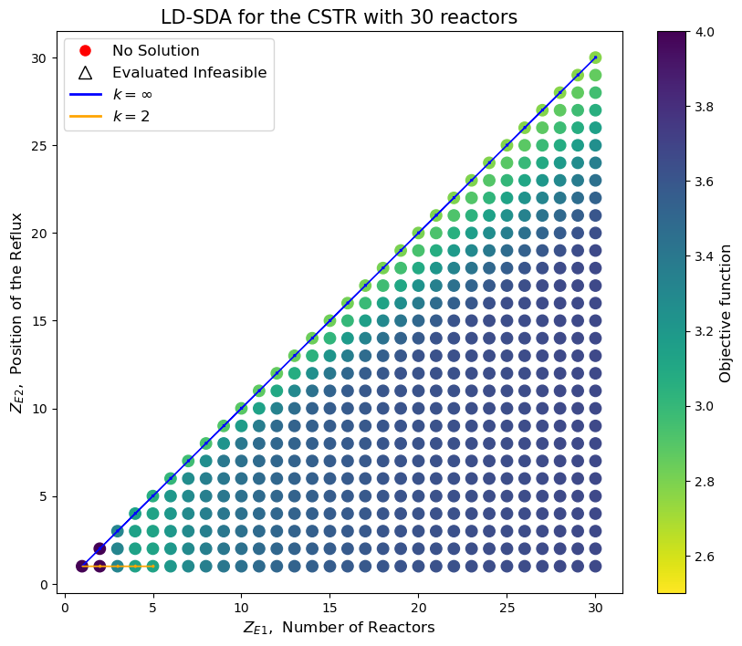
Figure 6: Paths and solutions found by the LD-SDA for a $N_{T}=30$ CSTR series; LD-SDA with $k=2$ converged on $[5,1]$ which is the local optimal point in the lattice; LD-SDA with $k=\infty$ proceeded to $[30,30]$.

For a reactor series superstructure with $N_{T}=30$, we performed external variable reformulation and fully enumerated the discrete points in a 30$\times$30 lattice. Notably, only the lower right triangle of the lattice is depicted, as points outside this region yield infeasible Boolean configurations. More specifically, these points indicate superstructures that have their recycle previous to an uninstalled reactor. Local optimality was verified with both neighborhoods, revealing local minima for $k=2$ neighborhood at $[5,1]$, $[5,3]$ and $[N,N]$ $\forall\$ $N\in\{5,\dots,29\}$, whereas the only locally optimal point for $k=\infty$ was $[30,30]$. Figure 6 illustrates the LD-SDA process for the 30 CSTR series, showing trajectories and local minimum points for all neighborhoods. The presence of multiple local optima with respect to both the $2$-neighborhood and the $\infty$-neighborhood suggests that this problem is neither separably convex nor integrally convex.

For the CSTR series, various solver approaches are applied across different numbers of potential reactors ($N_{T}$ ranging from 5 to 30). The solution approaches include MINLP reformulations, LBB, LOA, GLOA, and LD-SDA with two different neighborhoods. Figure 7 illustrates the comparison of solution times for each reactor superstructure size with different solvers. Notably, LD-SDA with $k=2$ neighborhoods failed to achieve optimal solutions within $0.1\%$ of the global optimum for any superstructure size, converging instead to the $[5,1]$ solution, as explained above. In contrast, methods that employed $k=\infty$ attained the global minimum. KNITRO was computationally more efficient than BARON when using $k=\infty$, as BARON, being a global solver, incurred higher in computational costs certifying global optimality for each NLP subproblem. Interestingly, even when using local solvers like KNITRO for the subproblem, $k=\infty$ allowed LD-SDA to converge to global optimal solutions. Among the logic-based methods in GDPopt, LBB for $N_{T}=5$ achieved the global optimum. GLOA reached globally optimal solutions up to $N_{T}=14$ but only when paired with the global NLP solver BARON. Comparing MINLP reformulations, HR outperformed BM, with KNITRO being the most efficient subsolver. While some MINLP reformulations exhibited faster solution times for smaller superstructures (up to 9 reactors), LD-SDA, particularly with KNITRO, surpassed them for larger networks (from 15 reactors onwards). This trend suggests that LD-SDA methods are particularly well-suited for solving larger optimization problems, where solving reduced subproblems offers a significant advantage over monolithic GDP-MINLP approaches.

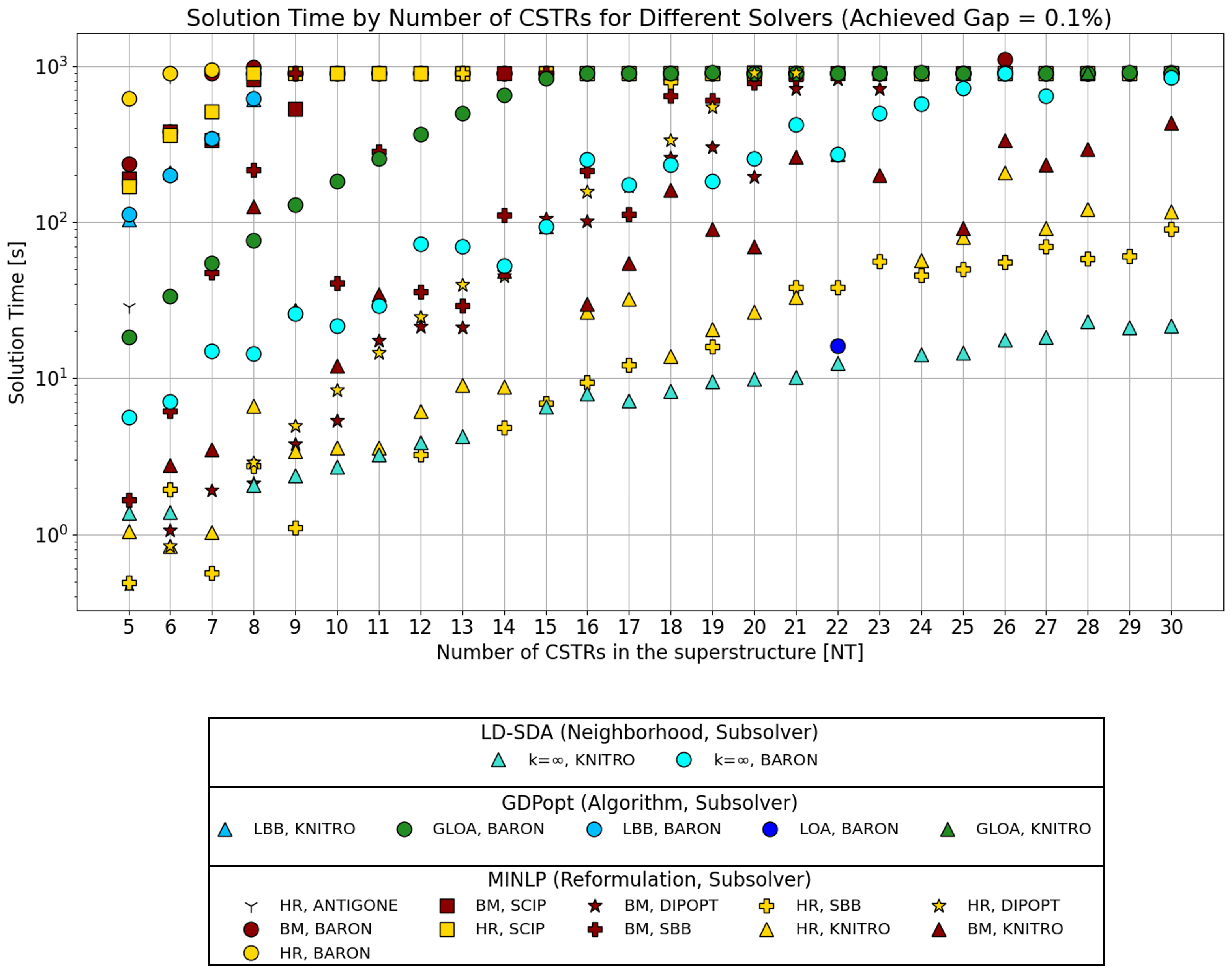
Figure 7: Computational time for different sizes of reactor network $N_{T}$ for various solution strategies. Solutions only accounted for being the analytically guaranteed global optimal solution (equivalent to the installing $N_{T}$ reactors since the minimum volume corresponds to $PFR=\lim_{N_{T}\to\infty}CSTR$).

Figure 8 compares different algorithmic alternatives derived from LD-SDA. These include the algorithm discussed so far (referred in this example as NLP LD-SDA) where Boolean variables are fixed from external variables, leading to NLP subproblems considering only relevant constraints. Another approach, which we refer to as MIP LD-SDA, is where inactive disjunctions are retained in subproblems, and mixed-binary reformulations (e.g., HR or BM) are applied to unresolved disjunctions, resulting in MINLP subproblems. The third alternative is Enumeration, which involves reformulating external variables, fixing (or not) Boolean variables, and enumerating all lattice points instead of traversing them via steepest descent optimization.

LD-SDA and Enumeration methods exhibited faster performance when the mixed-binary reformulation was omitted. The inclusion of MIP transformations led to additional solution time, emphasizing the efficiency of solving GDP problems directly where reduced subproblems with solely relevant constraints are considered. As anticipated, the Enumeration of external variables coupled with a proficient local solver like KNITRO achieved the global optimum. However, employing LD-SDA yielded the same result in significantly less time, showcasing the importance of navigating the lattice intelligently, like via discrete-steepest descent.

Among the LD-SDA approaches, $2$-neighborhood search methods were only effective when the tolerance gap between solutions was $10\%$, while $\infty$-neighborhood search methods performed consistently across both gap thresholds. The LD-SDA using $k=2$ neighborhood converges to a local minimum, which is more than $0.1\%$ away from the global optimal solution and, for larger instances, is beyond the $10\%$ optimality gap. Although LD-SDA with the $k=\infty$ neighborhood search required more time compared to $k=2$, it consistently converged to the global optimal point regardless of the superstructure size.

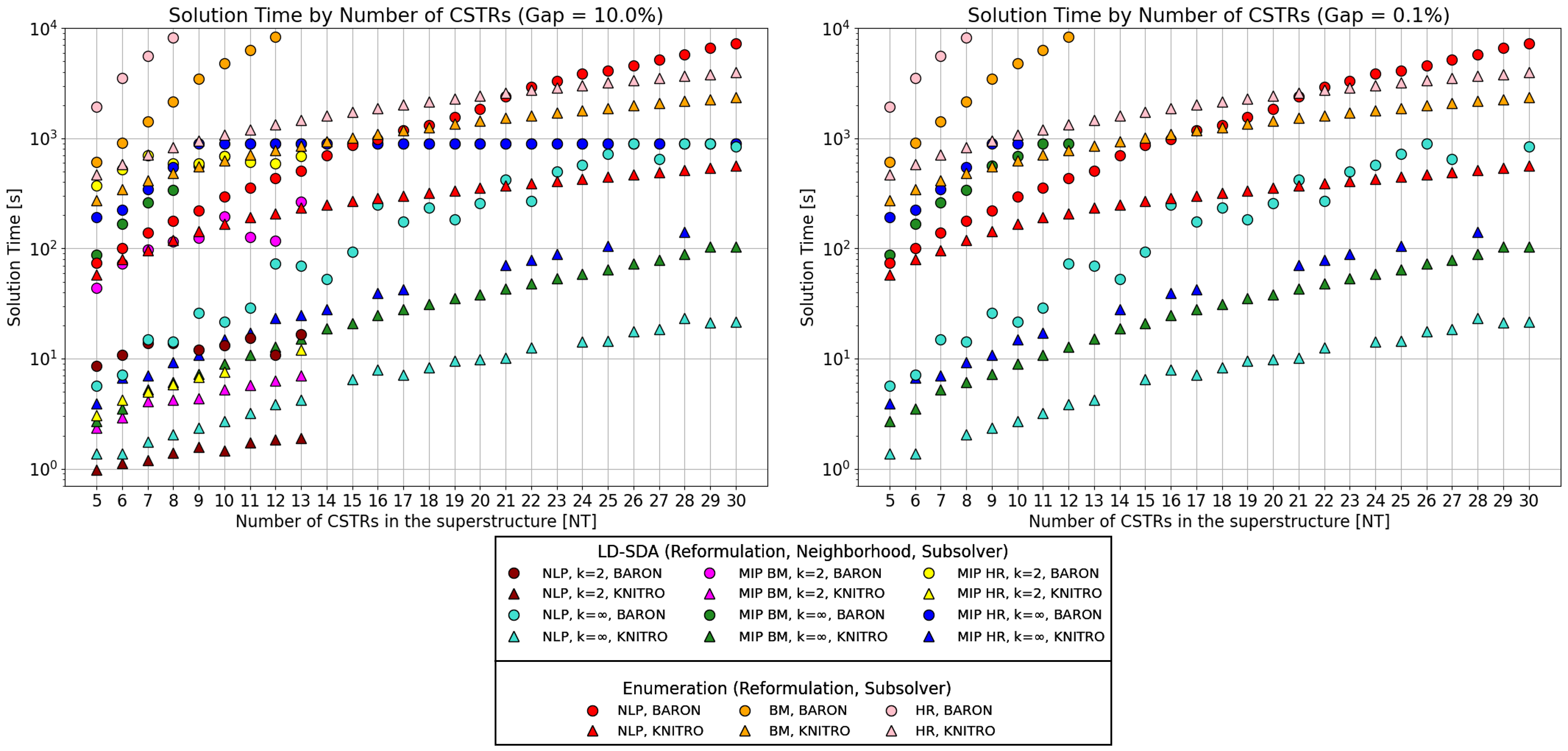
Figure 8: Solution times for CSTR superstructures using LD-SDA and Enumeration methods at different optimality gap: (left) $10\%$, (right) $0.1\%$).

5.2 Distillation Column Design for a Binary Mixture

We consider the single-unit operation design of an example distillation column in [60], which implements the simplified model provided by [61]. The objective is to design a distillation column to separate Toluene and Benzene while minimizing cost. There is a fixed cost associated with tray installation and an operational cost related to the condenser and reboiler duties. The feed conditions are 100 mol/s of an equimolar benzene-toluene mixture, with a minimum mole fraction of 0.95 benzene in the distillate and 0.95 toluene in the bottom. The constraints are the mass, equilibrium, summation, and heat (MESH) equations for each tray. Each column stage is modeled with thermodynamic and vapor-liquid equilibrium via Raoult’s law and Antoine’s equation. The continuous variables of this model are the flow rates of each component in the liquid and vapor phase and the temperatures in each tray, the reflux and boil-up ratio, and the condenser and reboiler heat duties. The logical variables are the existence of trays and the position of the reflux and boil-up flows. Furthermore, the existence of trays expressed only in terms of the position of the reflux and boil-up flows can be posed with a logical constraint. The reformulation of the Boolean variables to external variables is described in the figure shown in Appendix B.2. Previous studies from the literature  [60] set a maximum number of 17 potential trays and provide the initial position of the feed tray in the ninth stage (tray number 9).

The distillation column optimization uses the LD-SDA method with different neighborhoods for the search. The problem is initialized with a column that has the reflux at tray $16$ (top to bottom numbering, condenser being tray $17$ and the reboiler being tray $1$) and the boil-up at the second tray, which we represent as $[15,1]$. The configuration for initialization is shown in Figure 9(a), which corresponds to all possible trays being installed.

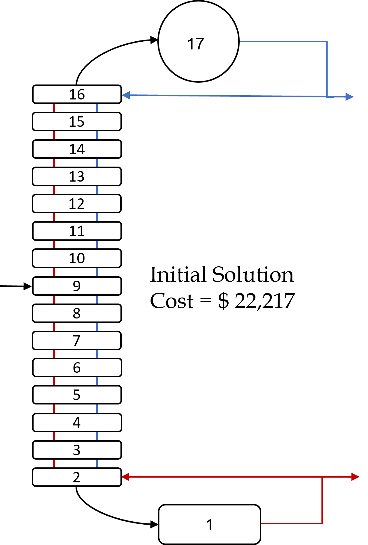
(a) Initial solution for the Distillation Column

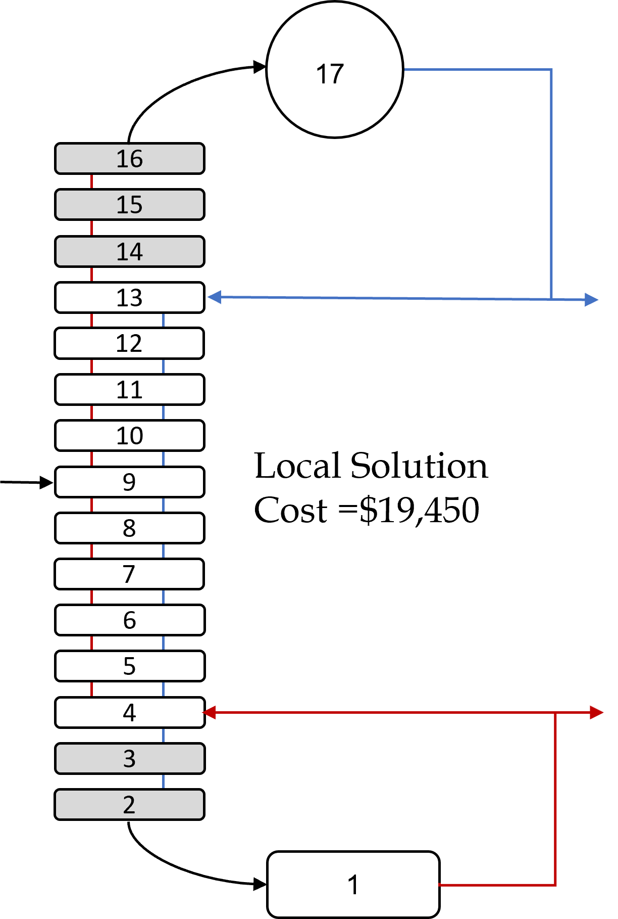
(b) Distillation Column Solution by LD-SDA $k=2$. Reference solution by [60] using GDP model

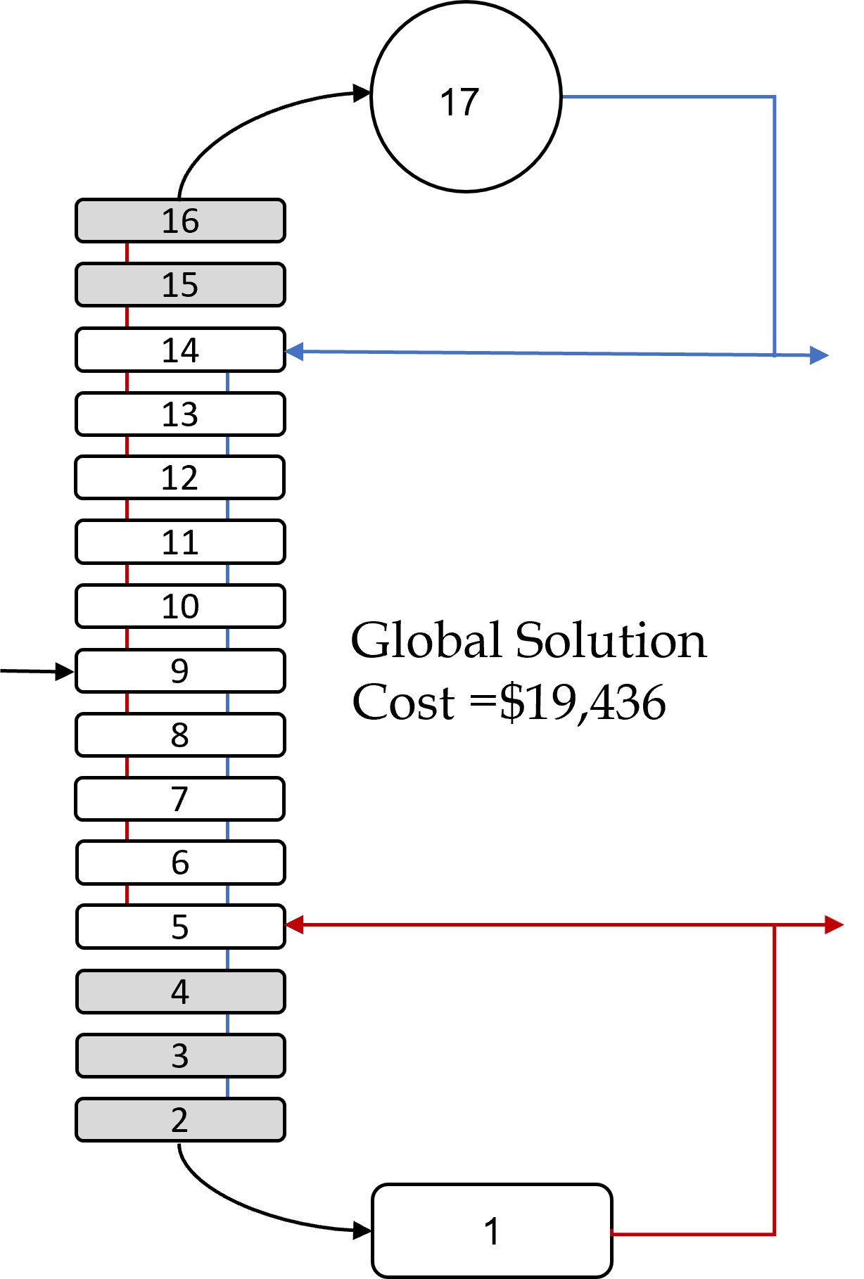
(c) Distillation Column Solution by LD-SDA $k=\infty$

Figure 9: Distillation Column design comparison between the initial, local, and global solutions.

For the $2$-neighborhood, the LD-SDA converges to external variable configuration $[12,3]$, with an objective value of $\$19,450$ in only 6.3 seconds using KNITRO as subsolver, resulting in the design shown in Figure 9(b). Note this is the exact same solution reported by the GDP model from the literature [60], which was solved using the LOA method.

Regarding the $\infty$-neighborhood, the algorithm terminates at $[13,4]$ with an objective of $\$19,346$ after 8.6 seconds using KNITRO as subsolver, yielding the column design shown in Figure 9(c). In this case, the LD-SDA found the best-known solution to this problem, also found through a complete enumeration over the external variables, which took 42.7 seconds using KNITRO as a subsolver. The same best-known solution could be found using GLOA with KNITRO as the NLP subsolver, but after 161.6 seconds. In our results of the binary mixture distillation column design, we successfully identified a better solution by applying the LD-SDA to the GDP model, surpassing the optimal values previously documented in the literature. This achievement highlights the efficacy of our approach, especially considering the limitations of the NLP formulation in guaranteeing global optimality, which we effectively navigated by employing the GDP framework.

The trajectories traversed by the LD-SDA with both neighborhoods mentioned are depicted in Figure 10. Similarly, Table 1 summarizes the previous design from the literature as well as the different columns obtained by the LD-SDA.

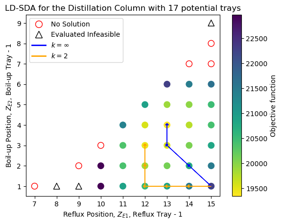
Figure 10: Algorithmic steps of LD-SDA when solving column example.

Table 1: Comparison of the optimal solution with the literature results and the LD-SDA solution.

Solution Method	LOA [60]	LD-SDA $\mathbf{k=2}$	LD-SDA $\mathbf{k=\infty}$
Objective [$]	19,450	19,449	19,346
Number of Trays	10	10	10
Feed Tray	6	6	5
Reflux ratio	2.45	2.45	2.01
Reboil ratio	2.39	2.39	2.00

5.3 Catalytic Distillation Column Design

Consider a catalytic distillation column design for the production of Ethyl tert-butyl ether (ETBE) from isobutene and ethanol. In this work, two models are considered: one that uses equilibrium-based modeling in each of the separation and reactive stages and another one that includes a rate-based description of the mass and energy transfer in all the stages [35]. These models maximize an economic objective by determining the position of separation and catalytic stages along the column, together with a Langmuir-Hinshelwood-Hougen-Watson kinetic model for the chemical reaction, MESH equations for each one of the stages, and hydraulic constraints for the column operation. The goal is to determine optimal operational variables such as reboiler and condenser heat duties and reflux ratio. Similarly, design variables such as column diameter, tray height, and downcomer specifications need to be defined. Finally, discrete design choices, meaning feed locations and positions of catalytic stages, must be selected. A detailed description of the models is given in [36, 62].

Previously in the literature, the economic annualized profit objective maximization of a catalytic distillation column to produce ETBE from butenes and ethanol was solved using a D-SDA [36]. Here, the authors demonstrated the difficulty of this design problem as several traditional optimization methods fail even to obtain a feasible solution [33, 35]. In these papers, the D-SDA was used to solve the problem as a MINLP by fixing binary variables and including constraints of the form $y_{ik}\mathbf{h}_{ik}(x)\leq 0$ to enforce the logic constraints. In this work, we demonstrate that approaching the problem disjunctively and employing LD-SDA leads to a faster solution of subproblems (as in Eq. (Sub)) as our method neglects the irrelevant and numerically challenging nonlinear constraints.

Table 2: Execution time of catalytic distillation optimal design and the rate-based model presented in [36] using KNITRO.

	Catalytic Distillation Column				Rate based Catalytic Distillation Column
Solution Method	D-SDA: [36]		LD-SDA: This work		D-SDA: [36]		LD-SDA: This work
Neighborhood	$k=2$	$k=\infty$	$k=2$	$k=\infty$	$k=2$	$k=\infty$	$k=2$	$k=\infty$
Objective [$/year]	22,410	22,410	22,410	22,410	–	–	23,443.2	23,443.2
Time [s]	12.49	12.52	4.29	4.25	–	–	1089.31	1061.18

These models were implemented in GAMS, hence, for this problem, the reformulation and implementations of the algorithms were custom-made, as they did not rely on our implementation of LD-SDA in Python. Given that only the relevant constraints were included for each problem, we could more efficiently obtain the same solution to each subproblem. More specifically, as shown in Table 2, the proposed LD-SDA method leads to speedups of up to 3x in this problem when using KNITRO as a subsolver. D-SDA was unable to even initialize the rate-based catalytic distillation column with KNITRO, while LD-SDA could find the optimal solution. Moreover, note that the previous results using the D-SDA were already beating state-of-the-art MINLP solution methods, further demonstrating the advantages of the LD-SDA.

An important distinction for the LD-SDA is that it does not include all the constraints in each iteration, given that subproblems are reduced after disjunctions are fixed. This implies that not all variables are present in all iterations, preventing a complete variable initialization as the algorithm progresses. These missing values for the variables might make converging these complex NLP problems challenging, explaining why the D-SDA and the LD-SDA sometimes yield different solutions. Moreover, the solver KNITRO reported that the initial point was infeasible for the more complex NLP problem involving rate-based transfer equations. Using that same initialization, yet using the logic-based D-SDA, the model could not only be started but it converged to the same optimal solution reported in [35].

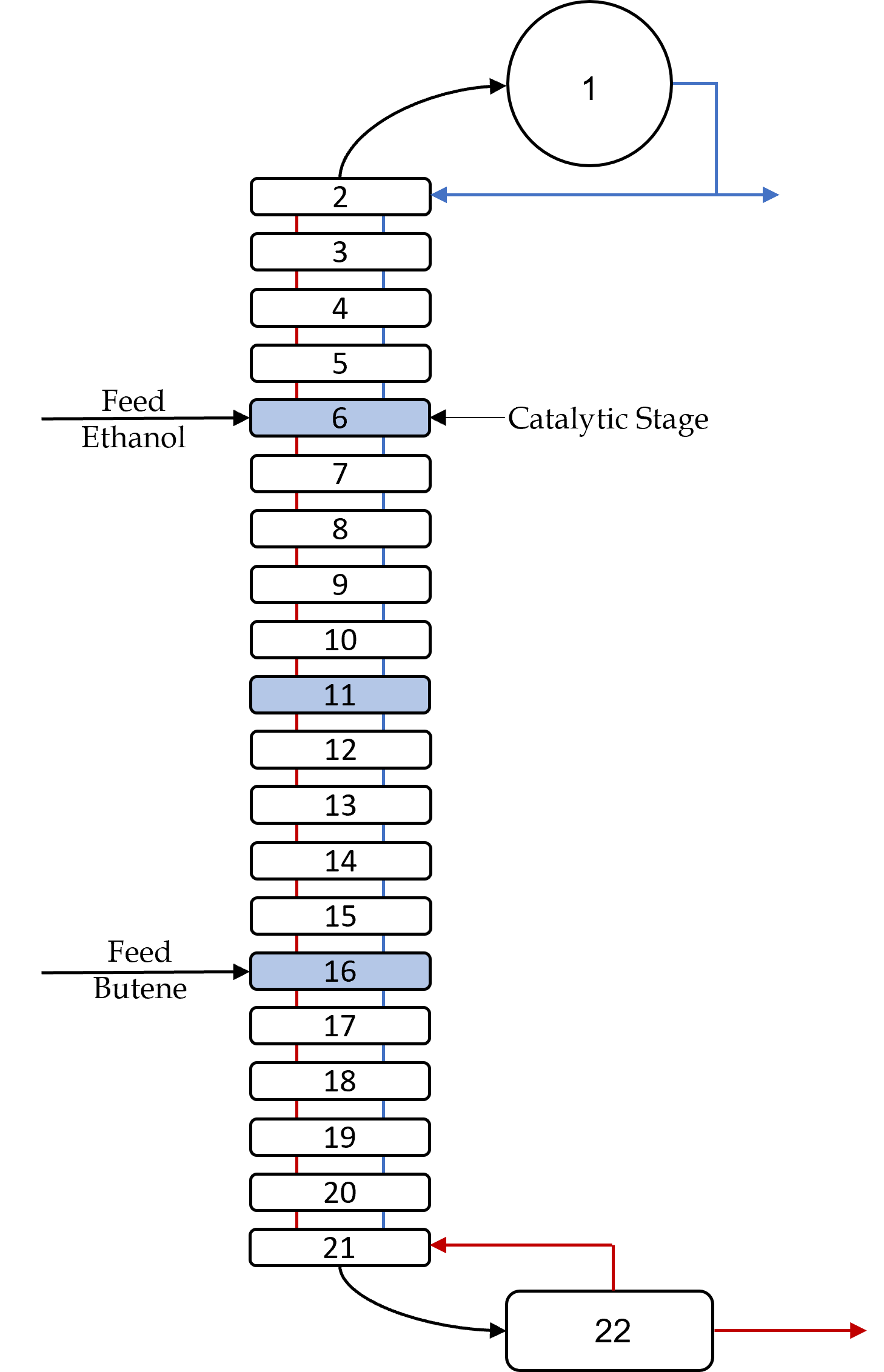
(a) Catalytic column superstructure.

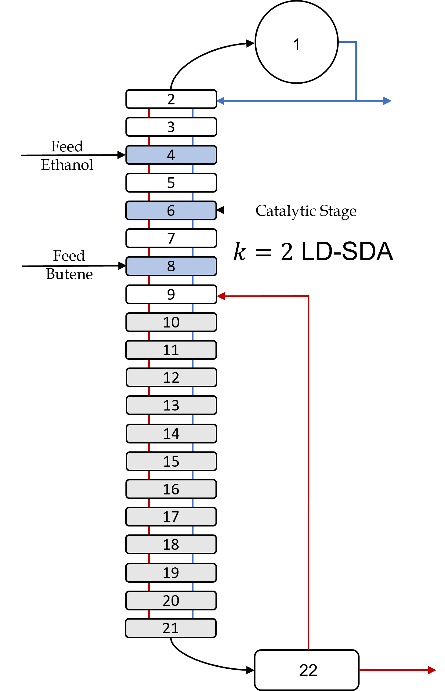
(b) LD-SDA with $k=2$ solution.

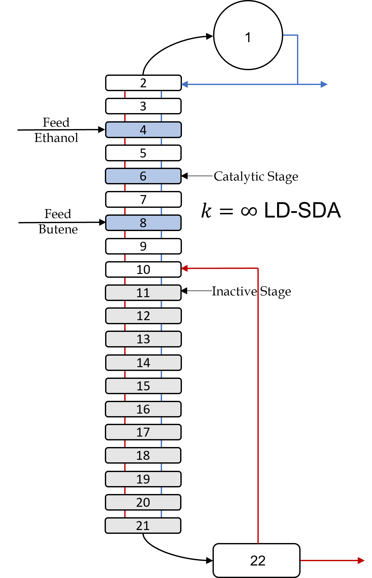
(c) LD-SDA with $k=\infty$ solution.

Figure 11: Solution design comparison of the catalytic distillation column problem between using the LD-SDA.

5.4 Optimal Design for Chemical Batch Processing

Consider an instance of the optimal design for chemical batch processing from [63] formulated as a GDP. This is a convexified GDP that aims to find the optimal design for multiproduct batch plants that minimizes the sum of exponential costs. In our example, the process has $3$ processing stages where fixed amounts of $q_{i}$ of $2$ products must be produced. The goal of the problem is to determine the number of parallel units $n_{j}$, the volume $v_{j}$ of each stage $j$, the batch sizes $b_{i}$, and the cycle time $tl_{i}$ of each product $i$. The given parameters of the problem are the time horizon $h$, cost coefficients $\alpha_{j},\beta_{j}$ for each stage $j$, size factors $s_{ij}$, and processing time $t_{ij}$ for product $i$ in stage $j$. The optimization model employs Boolean variables $Y_{kj}$ to indicate the presence of a stage, potentially representing three unit types: mixers, reactors, and centrifuges. The formulation of the model can be found in Appendix A.3 and the external variable reformulation of the Boolean variables is described in Appendix B.4.

The problem was initialized by setting the maximum number of units, i.e., $[3,3,3]$, for the number of mixers, reactors, and centrifuges, respectively. The algorithm terminates on a solution with objective $\$167,427$ with external variables $[2,2,1]$ for both $k=2$ or $k=\infty$ neighborhood alternatives in LD-SDA. The trajectories taken by both searches of the LD-SDA for the small batch problem are shown in Figure 12. This solution corresponds to the global optimal solution of the problem, hinting that convergence to global optimal solutions in convex GDP might be achieved even with $k=2$ in the Neighbor Search step. For this small problem, the solution times were negligible ($<2$ seconds). Still, this example is included to observe convergence to the same solution in a convex GDP problem using different neighborhoods.

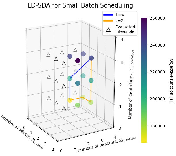
Figure 12: LD-SDA paths to optimal solution in the small batch scheduling case study.

6 Conclusions and Final Remarks

This work presented the Logic-based Discrete-Steepest Descent Algorithm (LD-SDA) as an optimization method for GDP problems with ordered Boolean variables, which often appear in process superstructure and single-unit design problems. The unique characteristics of the LD-SDA are highlighted, and its similarities with other existing logic-based methods are discussed. To verify the performance of the LD-SDA, we solved various GDP problems with applications in process systems engineering, such as reactor series volume minimization, binary distillation column design, rate-based catalytic distillation column design, and chemical batch process design. The LD-SDA demonstrated an efficient convergence toward high-quality solutions that outperformed state-of-the-art MINLP solvers and GDP solution techniques. The results show that LD-SDA is a valuable tool for solving GDP models with ordered Boolean variables.

Future research directions include utilizing the LD-SDA to solve larger and more challenging ordered GDPs. Similarly, we propose exploring theoretical convergence guarantees of the LD-SDA method, with a special focus on convex GDP problems and their relation to integrally convex problems in discrete analysis. Moreover, part of the future work involves the integration of the LD-SDA into the GDPOpt solver in Pyomo.GDP, making it available to more practitioners. Finally, we will study the parallelization of NLP solutions in the neighborhood search. The neighbor search can be faster by dividing the computation involved in solving NLP problems into multiple tasks that can be executed simultaneously, eventually improving LD-SDA performance.

The appendices show how the GDP models, such as reactors and chemical batch processing, are formulated. The objective functions and their algebraic and logical constraints are described for the model. Also, the reformulations of the Boolean Variables into External variables for the models are given in this section. There are some models which are described as figures.

Appendix A Generalized Disjunctive Programming formulations

This appendix includes the formulations of the examples of the problems solved in this manuscript as Generalized Disjunctive Programs (GDP).

A.1 Series of Reactors

Set of components (index i)

$$I=\{A,B\}$$ (6)

Set of units in the superstructure (index n, j)

$$N=\{1,...,NT\}$$ (7)

Existence of an unreacted feed in unit n

$$\begin{gathered}YF_{n}\in\{\textit{True, False}\}\;\;\forall\ n\in N\\ \text{If }YF_{n}=\textit{True}\implies\text{There is unreacted feed in reactor {n}}\end{gathered}$$ (8)

Existence of a recycle flow in unit n

$$\begin{gathered}YR_{n}\in\{\textit{True, False}\}\;\;\forall\ n\in N\\ \text{If }YR_{n}=\textit{True}\implies\text{There is recycle in reactor {n}}\end{gathered}$$ (9)

Unit operation in n: If at the current unit n every unit after it (from 1 to n) is not an unreacted feed or if the current unit n has the unreacted feed, then the unit is a CSTR (the opposite is also true)

$$\begin{gathered}YP_{n}\iff\left(\bigwedge_{j\in\{1,2,..n\}}\neg YF_{j}\right)\vee YF_{n}\;\;\forall\ n\in N\\ \text{If }YP_{n}=\textit{True}\implies\text{Unit {n} is a CSTR}\\ \text{If }YP_{n}=\textit{False}\implies\text{Unit {n} is a bypass}\end{gathered}$$ (10)

The unit must be a CSTR to include a recycle at n

$$YR_{n}\implies YP_{n}\;\;\forall\ n\in N$$ (11)

There is only one unreacted feed

$$\begin{gathered}\operatorname*{\underline{\bigvee}}_{n\in N}\end{gathered}YF_{n}$$ (12)

There is only one recycling stream.

$$\begin{gathered}\operatorname*{\underline{\bigvee}}_{n\in N}\end{gathered}YR_{n}$$ (13)

Unreacted feed unit: Partial mole balance

$$0=F0_{i}+FR_{i,NT}-F_{i,NT}+r_{i,NT}V_{NT}\;\;\forall\ i\in I$$ (14)

Unreacted feed unit: Continuity

$$0=Q_{F0}+Q_{FR,NT}-Q_{NT}$$ (15)

Reactor Sequence: Partial mole balance

$$0=F_{i,n+1}+FR_{i,n}-F_{i,n}+r_{i,n}V_{n}\;\;\forall\ n\in N\setminus\{NT\},\forall\ i\in I$$ (16)

Reactor Sequence: Continuity

$$0=Q_{n+1}+Q_{FR,n}-Q_{n}\;\;\forall\ n\in N\setminus\{NT\}$$ (17)

If unit n is a CSTR or a bypass

$$\left[\begin{gathered}YP_{n}\\ r_{A,n}Q_{n}^{2}=-kF_{A,n}F_{B,n}\\ r_{B,n}=-r_{A,n}\\ c_{n}=V_{n}\end{gathered}\right]\operatorname*{\underline{\bigvee}}\left[\begin{gathered}\neg YP_{n}\\ FR_{i,n}=0\;\;\forall\ i\in I\\ r_{i,n}=0\;\;\forall\ i\in I\\ Q_{FR,n}=0\\ c_{n}=0\end{gathered}\right]\forall\ n\in N$$ (18)

If there is recycle in before reactor n

$$\left[\begin{gathered}YR_{n}\\ FR_{i,n}=R_{i}\;\;\forall\ i\in I\\ Q_{FR,n}=Q_{R}\\ \end{gathered}\right]\operatorname*{\underline{\bigvee}}\left[\begin{gathered}\neg YR_{n}\\ FR_{i,n}=0\;\;\forall\ i\in I\\ Q_{FR,n}=0\\ \end{gathered}\right]\forall\ n\in N$$ (19)

Splitting point: Partial mole balance

$$0=F_{i,1}-P_{i}-R_{i}\;\;\forall\ i\in I$$ (20)

Splitting point: Continuity

$$0=Q_{1}-Q_{P}-Q_{R}$$ (21)

Splitting point: Additional constraint

$$0=P_{i}Q_{1}-F_{i,1}Q_{P}\;\;\forall\ i\in I$$ (22)

Product specification constraint

$$0.95Q_{P}=P_{B}$$ (23)

Volume constraint

$$V_{n}=V_{n-1}\;\;\forall\ n\in N\setminus\{1\}$$ (24)

Objective Function: Total reactor network volume

$$f_{OBJ}=\min\sum_{n\in N}{c_{n}}$$ (25)

A.2 Distillation Column Design

Set of trays (index t)

$$T=\{2,3,\dots,16\}$$ (26)

Set of composition (index c)

$$C=\{\text{Benzene, Toluene}\}$$ (27)

Existence of tray t

$$\begin{gathered}Y_{t}\in\{\textit{True, False}\}\;\;\forall\ t\in T\\ \text{If }Y_{i}=\textit{True}\implies\text{There exist a tray in stage {t}}\end{gathered}$$ (28)

Existence of boil-up flow in tray t

$$\begin{gathered}YB_{t}\in\{\textit{True, False}\}\;\;\forall\ t\in T\\ \text{If }YB_{t}=\textit{True}\implies\text{There is a boil-up flow in tray {t}}\end{gathered}$$ (29)

Existence of reflux flow in tray t

$$\begin{gathered}YR_{t}\in\{\textit{True, False}\}\;\;\forall\ t\in T\\ \text{If }YR_{i}=\textit{True}\implies\text{There is a reflux flow in tray {t}}\end{gathered}$$ (30)

There is only one boil-up flow in the distillation column.

$$\begin{gathered}\operatorname*{\underline{\bigvee}}_{t\in T}\end{gathered}YB_{t}$$ (31)

There is only one reflux flow in the distillation column.

$$\begin{gathered}\operatorname*{\underline{\bigvee}}_{t\in T}\end{gathered}YR_{t}$$ (32)

Tray $t$ is an equilibrium stage or a bypass, where $\mathbf{g}_{1}(\mathbf{x})$ contains equilibrium mass and energy balances, while $\mathbf{g}_{2}(\mathbf{x})$ contains a bypass material balance

$$\begin{bmatrix}Y_{t}\\ \mathbf{g}_{1}(\mathbf{x})=\mathbf{0}\\ y_{t,\text{active}}=1\end{bmatrix}\operatorname*{\underline{\bigvee}}\begin{bmatrix}\neg Y_{t}\\ \mathbf{g}_{2}(\mathbf{x})=\mathbf{0}\\ y_{t,\text{active}}=0\end{bmatrix},\quad\forall\ t\in T$$ (33)

If the reflux flow is on or above tray $t$ and the boil-up flow is on or below tray $t$, then tray $t$ is an equilibrium stage (the opposite is also $True$).

$$\left(\begin{gathered}{\bigvee}\\ \forall\ \tau\in\{t,t+1,\dots,16\}\end{gathered}YR_{\tau}\right)\land\left(\begin{gathered}{\bigwedge}\\ \forall\ \tau\in\{t,t+1,\dots,16\}\end{gathered}\neg YB_{\tau}\vee YB_{t}\right)\Longleftrightarrow Y_{t},\quad\forall\ t\in T$$ (34)

The reflux flow stage is not below the feed tray.

$$\begin{gathered}{\bigwedge}\\ \forall\ t\in\{2,3,\dots,8\}\end{gathered}\neg YR_{t}$$ (35)

The boil-up flow is not above the feed tray.

$$\begin{gathered}{\bigwedge}\\ \forall\ t\in\{10,11,\dots,17\}\end{gathered}\neg YB_{t}$$ (36)

The column has at least eight active trays.

$$\sum_{t\in T}y_{t,active}\geq 8$$ (37)

Tray 1 (reboiler), tray 9 (feed), and tray 17 (condenser) are equilibrium stages.

$$Y_{1}=True,\ Y_{9}=True,\ Y_{17}=True,$$ (38)

Benzene concentration constraint (distillate product)

$$X_{D,\text{Benzene}}\geq 0.95$$ (39)

Toluene concentration constraint (bottom product)

$$X_{B,\text{Toluene}}\geq 0.95$$ (40)

Bounds imposed over the reflux ratio $RF$

$$0.5\leq RF\leq 4$$ (41)

Bounds imposed over the Reboil ratio $RB$

$$1.3\leq RB\leq 4$$ (42)

Objective Function: Sum of the capital cost (number of active trays) and operating cost (reboiler and condenser duty), where $Q_{R}$ is the reboiler duty, $Q_{C}$ is the condenser duty, and the sum term over binary variables $y_{t,\text{active}}$ represents the total number of active trays.

$$f_{OBJ}=\min_{RF,RB,feedtray,N_{trays}}10^{3}\left((Q_{R}+Q_{C})+\sum_{t\in T}^{N_{trays}}y_{t,\text{active}}\right)$$ (43)

A.3 Small Batch Problem

Set of components (index i)

$$I=\{A,B\}$$ (44)

Set of stages (index j)

$$J=\{\text{mixer},\text{reactor},\text{centrifuge}\}$$ (45)

Set of potential number of parallel units for each stage (index k)

$$K=\{1,2,3\}$$ (46)

Existence of the parallel units for each stage j

$$\begin{gathered}Y_{kj}\in\{\textit{True, False}\}\;\forall\ k\in K,\ j\in J\\ \text{If }Y_{kj}=\textit{True}\implies\text{There are {k} parallel units in stage {j}}\end{gathered}$$ (47)

Only one of the parallel unit existence is $True$

$$\begin{gathered}\operatorname*{\underline{\bigvee}}_{j\in J}\end{gathered}Y_{kj}\quad\forall\ k\in K$$ (48)

Volume requirement in stage j

$$v_{j}\geq\ln(s_{ij})+b_{i}\quad\forall\ i\in I,\ j\in J$$ (49)

Cycle time for each product i

$$n_{j}+t_{Li}\geq\ln(t_{ij})\quad\forall\ i\in I,\ j\in J$$ (50)

Constraint for production time(horizon constraint)

$$\sum_{i\in I}Q_{i}\exp{(t_{Li}-b_{i})}\leq H$$ (51)

Relating number of units to $0-1$ variables

$$n_{j}=\sum_{k\in K}\gamma_{kj}\quad\forall\ j\in J$$ (52)

If only k parallel units exist in stage j

$$\begin{bmatrix}\begin{gathered}Y_{kj}\\ \gamma_{kj}=\ln{(k)}\\ \end{gathered}\end{bmatrix}\operatorname*{\underline{\bigvee}}\begin{bmatrix}\begin{gathered}\neg Y_{kj}\\ \gamma_{kj}={0}\\ \end{gathered}\end{bmatrix}\quad\forall\ k\in K,\ j\in J$$ (53)

Objective Function: the investment cost for setting the small batch system $[\$]$

$$f_{OBJ}=\min\sum_{j\in J}\alpha_{j}(\exp(n_{j}+\beta_{j}v_{j}))$$ (54)

Appendix B External variable reformulation for example problems

This appendix presents the external variable reformulation of the Boolean variables in the examples considered in this manuscript.

B.1 Series of Reactors Problem

$$YF_{n}=\begin{cases}True,\;\;\mathbf{z}_{E,1}=n\\ False,\;\;\text{otherwise}\end{cases}\forall\ n\in N$$ (B.1.1)

$$YR_{n}=\begin{cases}True,\;\;\mathbf{z}_{E,2}=n\\ False,\;\;\text{otherwise}\end{cases}\forall\ n\in N$$ (B.1.2)

$$X_{1}=\left\{\mathbf{z_{E}}\in\mathbb{Z}^{2}:\begin{gathered}1\leq\mathbf{{z}_{E,1}}\leq NT\\ 1\leq\mathbf{{z}_{E,2}}\leq NT\end{gathered}\right\}$$ (B.1.3)

$$X_{2}=\left\{\mathbf{{z}_{E}}\in\mathbb{Z}^{2}:\mathbf{{z}_{E,2}}-\mathbf{z_{E,1}}\leq 0\right\}$$ (B.1.4)

$$X=X_{1}\cap X_{2}=\left\{x_{E}\in\mathbb{Z}^{2}:\begin{gathered}1-\mathbf{{z}_{E,1}}\leq 0\\ \mathbf{{z}_{E,1}}-NT\leq 0\\ 1-\mathbf{{z}_{E,2}}\leq 0\\ \mathbf{{z}_{E,2}}-\mathbf{{z}_{E,1}}\leq 0\\ \end{gathered}\right\}$$ (B.1.5)

B.2 External Variable Reformulation for Distillation Column Problem

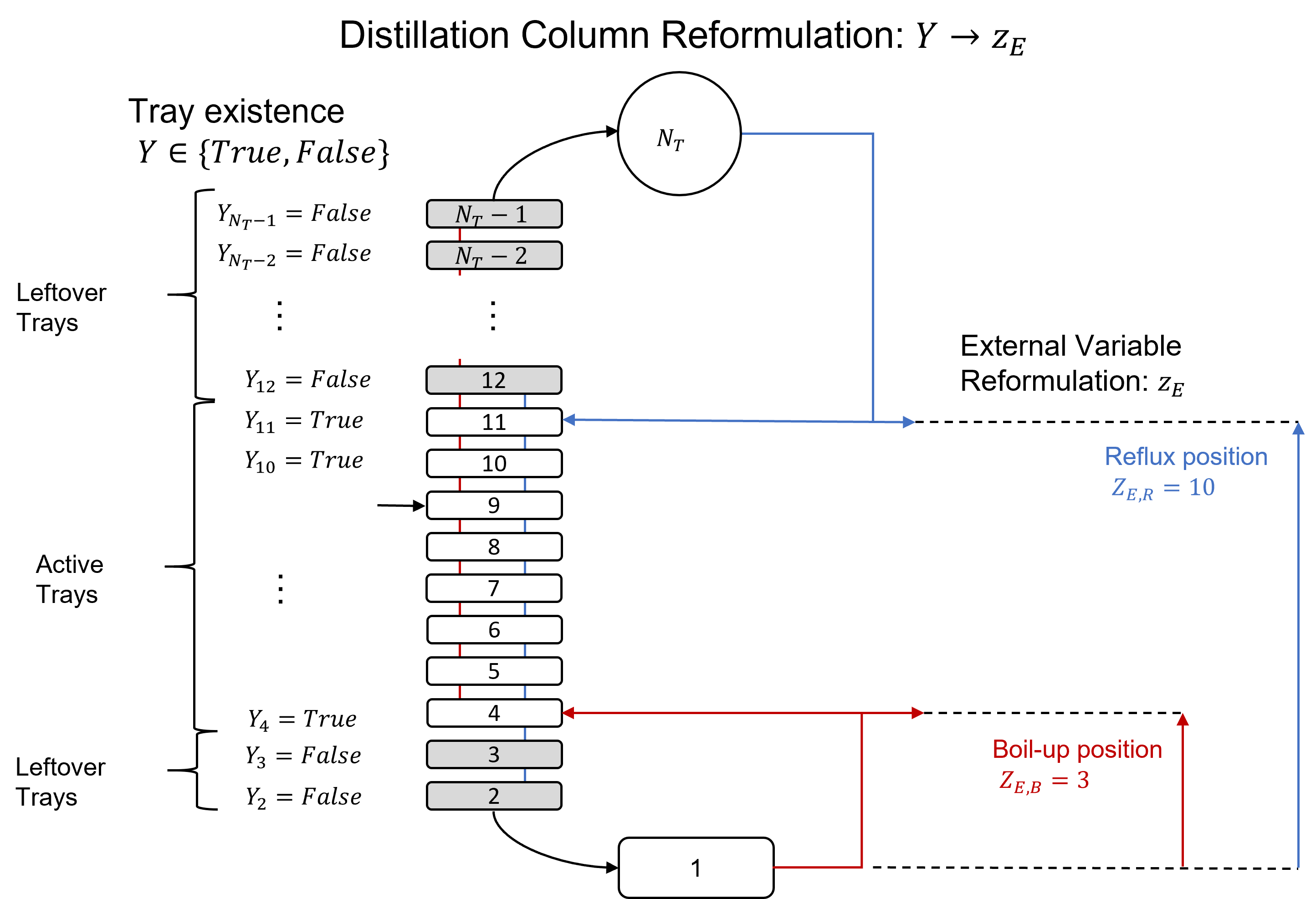
Figure 13: Example of distillation column external variable reformulation

$$YR_{t}=\begin{cases}True,\;\;\mathbf{z}_{\mathbf{E},\text{reflux}}=t-1\\ False,\;\;\text{otherwise}\end{cases}\forall\ t\in T$$ (B.2.1)

$$YB_{t}=\begin{cases}True,\;\;\mathbf{z}_{\mathbf{E},\text{boil-up}}=t-1\\ False,\;\;\text{otherwise}\end{cases}\forall\ t\in T$$ (B.2.2)

$$X_{1}=\left\{\mathbf{z}_{\mathbf{E}}\in\mathbb{Z}^{2}:\begin{gathered}1\leq\mathbf{z}_{\mathbf{E},\text{reflux}}\leq 15\\ 1\leq\mathbf{z}_{\mathbf{E},\text{boil-up}}\leq 15\\ \end{gathered}\right\}$$ (B.2.3)

B.3 Catalytic Distillation Column Problem

The external variable reformulation is equivalent to the one presented in [35] with Boolean variables instead of binary variables. We highlight in Figure 14 how these external variables are interpretable as relative positions of the ethanol feed, the butene feed, the catalytic stages and the boil-up.

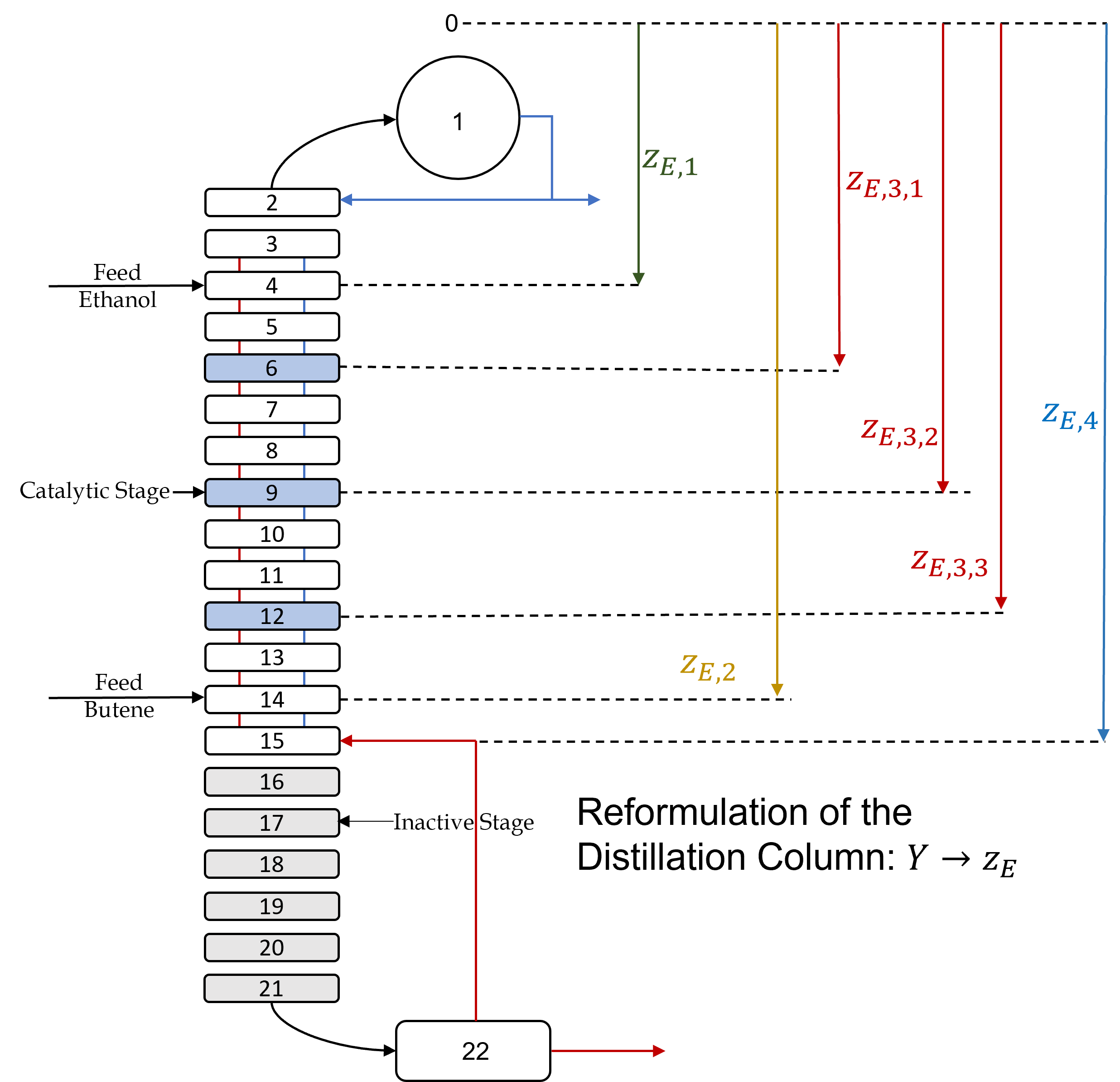
Figure 14: Example of catalytic distillation column external variable reformulation

B.4 Small Batch Problem

$$Y_{k,\text{mixer}}=\begin{cases}True,\;\;\mathbf{z}_{\mathbf{E},\text{mixer}}=k\\ False,\;\;\text{otherwise}\end{cases}\forall\ k\in K$$ (B.4.1)

$$Y_{k,\text{reactor}}=\begin{cases}True,\;\;\mathbf{z}_{\mathbf{E},\text{reactor}}=k\\ False,\;\;\text{otherwise}\end{cases}\forall\ k\in K$$ (B.4.2)

$$Y_{k,\text{centrifuge}}=\begin{cases}True,\;\;\mathbf{z}_{\mathbf{E},\text{centrifuge}}=k\\ False,\;\;\text{otherwise}\end{cases}\forall\ k\in K$$ (B.4.3)

$$X_{1}=\left\{\mathbf{z}_{\mathbf{E}}\in\mathbb{Z}^{3}:\begin{gathered}1\leq\mathbf{z}_{\mathbf{E},\text{mixer}}\leq K\\ 1\leq\mathbf{z}_{\mathbf{E},\text{reactor}}\leq K\\ 1\leq\mathbf{z}_{\mathbf{E},\text{centrifuge}}\leq K\end{gathered}\right\}$$ (B.4.4)

References

- [1] Ignacio Grossmann “Enterprise-wide optimization: A new frontier in process systems engineering” In AIChE Journal 51.7 Wiley Online Library, 2005, pp. 1846–1857
- [2] Oswaldo Andrés-Martínez and Luis A Ricardez-Sandoval “Integration of planning, scheduling, and control: A review and new perspectives” In The Canadian Journal of Chemical Engineering 100.9 Wiley Online Library, 2022, pp. 2057–2070
- [3] Luca Mencarelli, Qi Chen, Alexandre Pagot and Ignacio E Grossmann “A review on superstructure optimization approaches in process system engineering” In Computers & Chemical Engineering 136 Elsevier, 2020, pp. 106808
- [4] Yingjie Ma et al. “Simultaneous Synthesis and Design of Reaction–Separation–Recycle Processes Using Rigorous Models” In Industrial & Engineering Chemistry Research 60.19, 2021, pp. 7275–7290
- [5] Adrian Caspari et al. “The integration of scheduling and control: Top-down vs. bottom-up” In Journal of Process Control 91, 2020, pp. 50–62
- [6] Leo Liberti “Undecidability and hardness in mixed-integer nonlinear programming” In RAIRO-Operations Research 53.1 EDP Sciences, 2019, pp. 81–109
- [7] Ignacio E Grossmann “Review of nonlinear mixed-integer and disjunctive programming techniques” In Optimization and engineering 3 Springer, 2002, pp. 227–252
- [8] Jon Lee and Sven Leyffer “Mixed integer nonlinear programming” Springer Science & Business Media, 2011
- [9] Francisco Trespalacios and Ignacio E Grossmann “Review of mixed-integer nonlinear and generalized disjunctive programming methods” In Chemie Ingenieur Technik 86.7 Wiley Online Library, 2014, pp. 991–1012
- [10] Hector D Perez and Ignacio E Grossmann “Modeling hierarchical systems via nested generalized disjunctive programming” In Computer Aided Chemical Engineering 52 Elsevier, 2023, pp. 1373–1378
- [11] Laurence A Wolsey and George L Nemhauser “Integer and combinatorial optimization” John Wiley & Sons, 1999
- [12] Ramesh Raman and Ignacio E Grossmann “Modelling and computational techniques for logic based integer programming” In Computers & Chemical Engineering 18.7 Elsevier, 1994, pp. 563–578
- [13] Ignacio E Grossmann and Sangbum Lee “Generalized convex disjunctive programming: Nonlinear convex hull relaxation” In Computational optimization and applications 26.1 Springer, 2003, pp. 83–100
- [14] Egon Balas “Disjunctive programming” Springer, 2018
- [15] Metin Türkay and Ignacio E Grossmann “Logic-based MINLP algorithms for the optimal synthesis of process networks” In Computers & Chemical Engineering 20.8 Elsevier, 1996, pp. 959–978
- [16] Sangbum Lee and Ignacio E Grossmann “New algorithms for nonlinear generalized disjunctive programming” In Computers & Chemical Engineering 24.9-10 Elsevier, 2000, pp. 2125–2141
- [17] Hector Alejandro Pedrozo et al. “Optimal design of ethylene and propylene coproduction plants with generalized disjunctive programming and state equipment network models” In Computers & Chemical Engineering 149 Elsevier, 2021, pp. 107295
- [18] Xiang Zhang, Zhen Song and Teng Zhou “Rigorous design of reaction-separation processes using disjunctive programming models” In Computers & Chemical Engineering 111 Elsevier, 2018, pp. 16–26
- [19] Hend Ben Ali, Rubén Ruiz-Femenia and Ammar Ben Brahim “Design of once-through multistage flash process under the Generalized Disjunctive Programming framework” In 2017 International Conference on Green Energy Conversion Systems (GECS), 2017, pp. 1–7 IEEE
- [20] Qi Chen and Ignacio E Grossmann “Effective generalized disjunctive programming models for modular process synthesis” In Industrial & Engineering Chemistry Research 58.15 ACS Publications, 2019, pp. 5873–5886
- [21] Danlei Chen et al. “Synthesis of refrigeration system based on generalized disjunctive programming model” In Chinese journal of chemical engineering 26.8 Elsevier, 2018, pp. 1613–1620
- [22] Juan I Manassaldi, Miguel C Mussati, Nicolás J Scenna and Sergio F Mussati “Optimization of triple-pressure combined-cycle power plants by generalized disjunctive programming and extrinsic functions” In Computers & Chemical Engineering 146 Elsevier, 2021, pp. 107190
- [23] Jingyue Cui, Suela Jonuzaj and Claire S Adjiman “A Comprehensive Approach for the Design of Solvent-based Adhesive Products using Generalized Disjunctive Programming” In Computer Aided Chemical Engineering 44 Elsevier, 2018, pp. 427–432
- [24] Suela Jonuzaj, Aparana Gupta and Claire S Adjiman “The design of optimal mixtures from atom groups using Generalized Disjunctive Programming” In Computers & Chemical Engineering 116 Elsevier, 2018, pp. 401–421
- [25] Suela Jonuzaj and Claire S Adjiman “Designing optimal mixtures using generalized disjunctive programming: Hull relaxations” In Chemical Engineering Science 159 Elsevier, 2017, pp. 106–130
- [26] Ouyang Wu, Giancarlo Dalle Ave, Iiro Harjunkoski and Lars Imsland “A rolling horizon approach for scheduling of multiproduct batch production and maintenance using generalized disjunctive programming models” In Computers & Chemical Engineering Elsevier, 2021, pp. 107268
- [27] Daniel Ovalle et al. “Study of Different Formulations for the Multiperiod Blending Problem Applied to Lithium Recovery from Produced Water” In Computer Aided Chemical Engineering 52 Elsevier, 2023, pp. 1861–1866
- [28] Ming Li “Multi-periodic Refinery Scheduling Based on Generalized Disjunctive Programming” In Journal of Physics: Conference Series 1575.1, 2020, pp. 012195 IOP Publishing
- [29] Lijie Su et al. “Integrated scheduling of on-line blending and distribution of oil products in refinery operation” In Computer Aided Chemical Engineering 44 Elsevier, 2018, pp. 1213–1218
- [30] Maryam Mohammadi, Edgar Martı́n-Hernández, Mariano Martı́n and Iiro Harjunkoski “Modeling and Analysis of Organic Waste Management Systems in Centralized and Decentralized Supply Chains Using Generalized Disjunctive Programming” In Industrial & Engineering Chemistry Research 60.4 ACS Publications, 2021, pp. 1719–1745
- [31] Cristiana Lara and Ignacio Grossmann “Global optimization algorithm for multi-period design and planning of centralized and distributed manufacturing networks” In Computer Aided Chemical Engineering 43 Elsevier, 2018, pp. 1261–1262
- [32] Maria Analia Rodriguez, Jorge Marcelo Montagna, Aldo Vecchietti and Gabriela Corsano “Generalized disjunctive programming model for the multi-period production planning optimization: An application in a polyurethane foam manufacturing plant” In Computers & Chemical Engineering 103 Elsevier, 2017, pp. 69–80
- [33] David A Liñán, David E Bernal, Luis A Ricardez-Sandoval and Jorge M Gómez “Optimal design of superstructures for placing units and streams with multiple and ordered available locations. Part I: A new mathematical framework” In Computers & Chemical Engineering 137 Elsevier, 2020, pp. 106794
- [34] Kazuo Murota “Discrete convex analysis” In Mathematical Programming 83.1 Springer, 1998, pp. 313–371
- [35] David A Liñán, David E Bernal, Luis A Ricardez-Sandoval and Jorge M Gómez “Optimal design of superstructures for placing units and streams with multiple and ordered available locations. Part II: Rigorous design of catalytic distillation columns” In Computers & Chemical Engineering 139 Elsevier, 2020, pp. 106845
- [36] David A Liñán, David E Bernal, Jorge M Gómez and Luis A Ricardez-Sandoval “Optimal synthesis and design of catalytic distillation columns: A rate-based modeling approach” In Chemical Engineering Science 231 Elsevier, 2021, pp. 116294
- [37] David E Bernal et al. “Process Superstructure Optimization through Discrete Steepest Descent Optimization: a GDP Analysis and Applications in Process Intensification” In Computer Aided Chemical Engineering 49 Elsevier, 2022, pp. 1279–1284
- [38] David A Liñán and Luis A Ricardez-Sandoval “Discrete-Time Network Scheduling and Dynamic Optimization of Batch Processes with Variable Processing Times through Discrete-Steepest Descent Optimization” In Industrial & Engineering Chemistry Research ACS Publications, 2024
- [39] Paola Favati “Convexity in nonlinear interger programming” In Ricerca operativa 53, 1990, pp. 3–44
- [40] Michael L Bynum et al. “Pyomo-optimization modeling in python” Springer, 2021
- [41] Qi Chen et al. “Pyomo. GDP: an ecosystem for logic based modeling and optimization development” In Optimization and Engineering Springer, 2021, pp. 1–36
- [42] Ignacio E Grossmann and Francisco Trespalacios “Systematic modeling of discrete-continuous optimization models through generalized disjunctive programming” In AIChE Journal 59.9 Wiley Online Library, 2013, pp. 3276–3295
- [43] David E Bernal Neira and Ignacio E Grossmann “Convex mixed-integer nonlinear programs derived from generalized disjunctive programming using cones” In Computational Optimization and Applications Springer, 2024, pp. 1–62
- [44] Kevin C Furman, Nicolas W Sawaya and Ignacio E Grossmann “A computationally useful algebraic representation of nonlinear disjunctive convex sets using the perspective function” In Computational Optimization and Applications 76.2 Springer, 2020, pp. 589–614
- [45] Marco A Duran and Ignacio E Grossmann “An outer-approximation algorithm for a class of mixed-integer nonlinear programs” In Mathematical programming 36 Springer, 1986, pp. 307–339
- [46] Angelos Tsoukalas and Alexander Mitsos “Multivariate mccormick relaxations” In Journal of Global Optimization 59.2-3 Springer, 2014, pp. 633–662
- [47] Kazuo Murota and Akihisa Tamura “Recent progress on integrally convex functions” In Japan Journal of Industrial and Applied Mathematics Springer, 2023, pp. 1–55
- [48] David A Liñán and Luis A Ricardez-Sandoval “Optimal design and dynamic transitions of multitask catalytic distillation columns: A Discrete-Steepest Descend Framework” In Chemical Engineering and Processing-Process Intensification 180 Elsevier, 2022, pp. 108655
- [49] András Frank and Kazuo Murota “Decreasing minimization on M-convex sets: algorithms and applications” In Mathematical Programming 195.1-2 Springer, 2022, pp. 1027–1068
- [50] Krzysztof Ciesielski “Set theory for the working mathematician” Cambridge University Press, 1997
- [51] Scott P Stevens and Susan W Palocsay “Teaching use of binary variables in integer linear programs: Formulating logical conditions” In INFORMS Transactions on Education 18.1 INFORMS, 2017, pp. 28–36
- [52] Balasubramanian Ram and Sanjiv Sarin “An algorithm for the 0-1 equality knapsack problem” In Journal of the Operational Research Society 39.11 Taylor & Francis, 1988, pp. 1045–1049
- [53] Nikolaos V Sahinidis “BARON: A general purpose global optimization software package” In Journal of global optimization 8 Springer, 1996, pp. 201–205
- [54] Tobias Achterberg “SCIP: solving constraint integer programs” In Mathematical Programming Computation 1 Springer, 2009, pp. 1–41
- [55] Ruth Misener and Christodoulos A Floudas “ANTIGONE: algorithms for continuous/integer global optimization of nonlinear equations” In Journal of Global Optimization 59.2-3 Springer, 2014, pp. 503–526
- [56] David E Bernal, Stefan Vigerske, Francisco Trespalacios and Ignacio E Grossmann “Improving the performance of DICOPT in convex MINLP problems using a feasibility pump” In Optimization Methods and Software 35.1 Taylor & Francis, 2020, pp. 171–190
- [57] Michael R Bussieck and Arne Drud “SBB: A new solver for mixed integer nonlinear programming” In Talk, OR, 2001
- [58] Richard H Byrd, Jorge Nocedal and Richard A Waltz “Knitro: An integrated package for nonlinear optimization” In Large-scale nonlinear optimization Springer, 2006, pp. 35–59
- [59] Arne Stolbjerg Drud “CONOPT—a large-scale GRG code” In ORSA Journal on computing 6.2 INFORMS, 1994, pp. 207–216
- [60] Jaffer H Ghouse et al. “A comparative study between GDP and NLP formulations for conceptual design of distillation columns” In Computer Aided Chemical Engineering 44 Elsevier, 2018, pp. 865–870
- [61] Jennifer R Jackson and Ignacio E Grossmann “A disjunctive programming approach for the optimal design of reactive distillation columns” In Computers & Chemical Engineering 25.11-12 Elsevier, 2001, pp. 1661–1673
- [62] David E Bernal, Carolina Carrillo-Diaz, Jorge M Gómez and Luis A Ricardez-Sandoval “Simultaneous design and control of catalytic distillation columns using comprehensive rigorous dynamic models” In Industrial & Engineering Chemistry Research 57.7 ACS Publications, 2018, pp. 2587–2608
- [63] Gary R Kocis and Ignacio E Grossmann “Global optimization of nonconvex mixed-integer nonlinear programming (MINLP) problems in process synthesis” In Industrial & engineering chemistry research 27.8 ACS Publications, 1988, pp. 1407–1421