WSU-HEP-2402

May 8, 2024

Quasielastic Lepton-Nucleus Scattering and the Correlated Fermi Gas Model

Bhubanjyoti Bhattacharya^(a,b), Sam Carey^(b), Erez O. Cohen^(c), Gil Paz^(b)
(a) Department of Natural Sciences,
Lawrence Technological University, Southfield, Michigan 48075, USA
^(b) Department of Physics and Astronomy,
Wayne State University, Detroit, Michigan 48201, USA
^(c) Physics Department,
Nuclear Research Center - Negev,
P.O. Box 9001, 84190 Beer-Sheva, Israel

The neutrino research program in the coming decades will require improved precision. A major source of uncertainty is the interaction of neutrinos with nuclei that serve as targets for such experiments. Broadly speaking, this interaction often depends, e.g., for charge-current quasi-elastic scattering, on the combination of “nucleon physics”, expressed by form factors, and “nuclear physics”, expressed by a nuclear model. It is important to get a good handle on both. We present a fully analytic implementation of the Correlated Fermi Gas Model for electron-nucleus and charge-current quasi-elastic neutrino-nucleus scattering. The implementation is used to compare separately form factors and nuclear model effects for both electron-carbon and neutrino-carbon scattering data.

1 Introduction

Current and upcoming experiments involving lepton-nucleon scattering aim to precisely measure parameters in the Standard Model (SM) Lagrangian that describe leptonic interactions as well as to uncover non-standard neutrino interactions (NSI). Such precision measurements require a better control of systematic uncertainties in lepton-nucleus interactions. The cross-section for a charged lepton or a charge-current quasi-elastic (CCQE) neutrino scattering off a nucleus is determined by folding the lepton-quark interaction twice. Each folding gives rise to a source of systematic uncertainty. The first involves nucleon form factors needed to fold the lepton-quark interaction into the lepton-nucleon interaction. The result is the scattering cross-section on a single nucleon. The second folding is needed in going from the nucleon to the nuclear level, which involves a nuclear model and results in the cross-section on a nucleus consisting of multiple nucleons. Ideally, we would like to have separately a good control for each source of uncertainty.

It can be argued that the majority of the research in this field has focused on the nuclear level, where the nucleon level has received less study. This seems plausible for uncertainties arising from the electromagnetic form factors, since they can be extracted from electron-nucleon scattering, see, for example, the parameterizations in [1] and [2]. Uncertainties from the axial form factor are much harder to control. Historically, a dipole form factor was assumed for the axial form factor. For example, the comparative study [3], based on [4], compared six nuclear models: Benhar’s spectral function with and without the final-state interactions [5, 6, 7, 8], the Valencia spectral function [9, 10, 11, 12], the GiBUU model [13, 14], and the local and global Fermi gas models, all using the dipole model for the axial form factor [4].

The dipole model is not motivated from first principles and its usage can underestimate the uncertainties. This issue was highlighted in the MiniBooNE analysis [15] that seemed to require a higher axial mass than the preceding world-average value to explain the data. In [16, 17] a $z$-expansion based parametrization was introduced for the axial form factor. Assuming a definite nuclear model, namely, the relativistic Fermi gas (RFG) model [18], an axial mass was extracted from the MiniBooNE data using $z$-expansion based parametrization that was consistent with the preceding world-average values.

In the RFG model a nucleon within a nucleus is assumed to occupy momentum states only up to the Fermi momentum. Data from the last two decades have shown that this is not the case. Inclusive measurements involving large momentum transfer ($Q^{2}>1.5\,$ GeV²), showed that approximately $20\%$ of nucleons have momentum greater than the Fermi momentum [19, 20, 21]. Almost all high-momentum nucleons appear in short-range correlated (SRC) pairs, predominantly neutron-proton ones, and contribute most of the kinetic energy carried by nucleons in nuclei. Exclusive measurements on ¹²C and ⁴He have led to direct observations of such SRC pairs [22, 23, 24, 25, 26]. An extension of the RFG model that takes into account the high momentum tail beyond the nuclear Fermi momentum due to SRC pairing is the Correlated Fermi Gas (CFG) model suggested in [27]. In the CFG model, the nucleon momentum distribution is constant below the Fermi momentum and has a small high-momentum tail above the Fermi momentum.

The CFG model has been used to study the equation of state of nucleonic stars and its effects on stellar properties such as maximum mass and particle fraction[28, 29, 30, 31]. The CFG model has also been implemented to study the EMC effect, where the quark-gluon structure of a nucleon bound in an atomic nucleus is modified by the surrounding nucleons [32]. One goal of this paper is to present a fully analytic implementation of the CFG model for electron-nucleus and CCQE neutrino-nucleus scattering.

A second goal of this paper is to use this implementation to compare separately form factors and nuclear model effects for both electron-carbon and neutrino-carbon scattering data. Lack of such a control is both a long standing issue and a current topic. The first arises from the fact that many explanations for the MiniBooNE data [15] assumed the dipole axial form factor model and only tried to modify the nuclear effects. The studies of [16, 17] fixed the nuclear model and allowed for a flexible axial form factor. The lack of control is a current topic since in the last few years many extractions of the axial from factors from experimental data [34, 35] and lattice QCD [36, 37, 38, 39, 40] became available. A better control on the axial form factor will potentially allow to separate the nucleon and nuclear effects.

The structure of the paper is as follows. In section 2 we review the relation between the cross section and the nuclear tensor, and present the construction of the nuclear tensor using the nucleon form factors for the RFG and CFG models. In section 3 we present the analytic implementation of the CFG model for lepton-nucleus scattering. We compare the CFG predictions to electron-carbon data in section 4.1 and neutrino MiniBooNE data in section 4.2. For both we consider separately form factor effects, by comparing different form factor parameterizations, and nuclear effects, by comparing the RFG and CFG models. We summarize our findings in section 5. Some more technical details of the paper are relegated to the appendices.

2 Models

2.1 Lepton-nucleus cross section

We study processes in which an incoming lepton, neutral or charged, with four-momentum $k$ that scatters to a lepton with four-momentum $k^{\prime}$ off a target with four-momentum $p^{T}$. The differential cross section is expressed in terms of the nuclear tensor $W_{\mu\nu}$ defined below. Considering the possibility of both vector and axial currents, we can decompose $W_{\mu\nu}$ as a linear combination of scalar functions $W_{i}$ as [16]

$$W_{\mu\nu}=-g_{\mu\nu}W_{1}+\frac{p_{\mu}^{T}p_{\nu}^{T}}{m_{T}^{2}}W_{2}-\frac{i\epsilon_{\mu\nu\rho\sigma}p_{T}^{\rho}p_{T}^{\sigma}}{2m_{T}^{2}}W_{3}+\frac{q_{\mu}q_{\nu}}{m_{T}^{2}}W_{4}+\frac{p_{\mu}^{T}q_{\nu}+q_{\mu}p_{\nu}^{T}}{2m_{T}^{2}}W_{5}\,,$$ (1)

where $q=k-k^{\prime}$ and $m_{T}$ is the target mass. Defining $E_{\ell}\equiv{k^{\prime}}^{0}$ and $\vec{P}_{\ell}\equiv\vec{k}^{\prime}$ the energy and momentum of the final state lepton, the (anti-)neutrino-nucleus cross section is [16]

$$\frac{d\sigma^{\,\nu}_{\rm nuclear}}{dE_{\ell}\,d\cos\theta_{\ell}}=\frac{G_{F}^{2}|\vec{P}_{\ell}|}{16\pi^{2}\,m_{T}}\Bigg{\{}2(E_{\ell}-|\vec{P}_{\ell}|\cos\theta_{\ell})\,W_{1}+(E_{\ell}+|\vec{P}_{\ell}|\cos\theta_{\ell})W_{2}\\ \pm\frac{1}{m_{T}}\Big{[}(E_{\ell}-|\vec{P}_{\ell}|\cos\theta_{\ell})(E_{\nu}+E_{\ell})-m^{2}_{\ell}\Big{]}W_{3}+\frac{m_{\ell}^{2}}{m_{T}^{2}}(E_{\ell}-|\vec{P}_{\ell}|\cos\theta_{\ell})W_{4}-\frac{m_{\ell}^{2}}{m_{T}}\,W_{5}\Bigg{\}}\,,$$ (2)

where the upper (lower) sign is for neutrino (anti-neutrino) scattering.

Neglecting the electron mass, the electron-nucleus cross section is

$$\frac{d\sigma^{\,e}_{\rm nuclear}}{dE_{\ell}\,d\cos\theta_{\ell}}=\frac{\alpha^{2}E_{\ell}^{2}}{2q^{4}\,m_{T}}\Big{[}2W_{1}(1-\cos\theta_{\ell})+W_{2}(1+\cos\theta_{\ell})\Big{]}.$$ (3)

The nuclear tensor $W_{\mu\nu}$ is formally related to matrix elements of the vector and axial current between the initial and final nuclear states. We can relate it to the single nucleon tensor, $H_{\mu\nu}$ for both the RFG and CFG models by using a “statistical” approach presented explicitly in [16]. Denote by $n_{i}(\bm{p})$ the momentum distribution of the initial nucleon momentum $\bm{p}$. The final-state nucleon momentum $\bm{p}^{\prime}$ phase space is limited by a factor of $\left[1-n_{f}(\bm{p^{\prime}})\right]$ from the Fermi-Dirac statistics. The nuclear tensor $W_{\mu\nu}$ can be expressed in terms of the nucleon tensor $H_{\mu\nu}$ as follows,

$$W_{\mu\nu}=\int\frac{d^{3}p}{(2\pi)^{3}}\,\frac{m_{T}}{E_{p}}\,2Vn_{i}(\bm{p})\int\frac{d^{3}p^{\prime}}{(2\pi)^{3}2E_{p^{\prime}}}(2\pi)^{4}\delta^{4}(p-p^{\prime}+q)H_{\mu\nu}\left[1-n_{f}(\bm{p^{\prime}})\right]\,,$$ (4)

see [16] for details. Accounting for two possible spin states, the number of nucleons $N$ of a certain type, namely, protons or neutrons, determines the normalization factor $V$ as

$$N=\int\frac{d^{3}p}{(2\pi)^{3}}\,2Vn_{i}(\bm{p}).$$ (5)

In the following we use $N=A/2$, where $A$ is the total number of nucleons.

Since we will not consider the kinematics of the final state nucleon in this paper, we can integrate over $d^{3}p^{\prime}$ using the three-momentum delta function. We also incorporate a binding energy, $\epsilon_{b}$, by the replacements

$$p^{0}\to\epsilon_{\bm{p}}\equiv E_{\bm{p}}-\epsilon_{b}\,,\quad p^{\prime 0}\to\epsilon^{\prime}_{\bm{p}^{\prime}}\equiv E_{\bm{p}^{\prime}}\,,$$ (6)

where $E_{\bm{p}}\equiv\sqrt{m_{N}^{2}+|\bm{p}|^{2}}$. The resulting relation between $W_{\mu\nu}$ and $H_{\mu\nu}$ is [16]

$$W_{\mu\nu}\equiv \int d^{3}{p}\,f({\bm{p}},q^{0},\bm{q})H_{\mu\nu}(\epsilon_{\bm{p}},\bm{p};q^{0},\bm{q})\,,$$ (7)

with

$$f({\bm{p}},q^{0},\bm{q})=\frac{m_{T}V}{4\pi^{2}}\,n_{i}(\bm{p})[1-n_{f}(\bm{p}+\bm{q})]\frac{\delta(\epsilon_{\bm{p}}-\epsilon^{\prime}_{\bm{p}+\bm{q}}+q^{0})}{\epsilon_{\bm{p}}\epsilon^{\prime}_{\bm{p}+\bm{q}}}\,.$$ (8)

We discuss $f({\bm{p}},q^{0},\bm{q})$ for the RFG and CFG cases below. The nucleon tensor $H_{\mu\nu}$ is given by

$$H_{\mu\nu}={\rm Tr}[(\not{p}^{\prime}+m_{p^{\prime}})\Gamma_{\mu}(q)(\not{p}+m_{p})\bar{\Gamma}_{\nu}(q)]\,,$$ (9)

where $\Gamma_{\mu}(q)$ is defined via the matrix element of the electromagnetic or charged weak current $J_{\mu}$ as

$$\langle p^{\prime}|J_{\mu}|p\rangle =\bar{u}(p^{\prime})\Gamma_{\mu}(q)u(p)\,.$$ (10)

$\Gamma_{\mu}(q)$ can be expressed in term of form factors:

$$\Gamma_{\mu}(q)=\gamma_{\mu}F_{1}(q^{2})+\frac{i}{2m_{N}}\sigma_{\mu\nu}q^{\nu}F_{2}(q^{2})+\gamma_{\mu}\gamma_{5}F_{A}(q^{2})+\frac{q_{\mu}}{m_{N}}\gamma_{5}F_{P}(q^{2})\,,$$ (11)

where we assume time-reversal invariance. For neutrino scattering we also assume isospin symmetry, that allows to relate the neutron-to-proton $F_{1,2}$ to the electromagnetic form factors $F_{1,2}$ of the proton and neutron. For charged-lepton scattering, the nucleon mass is replaced by the mass of the proton ($m_{p}$) or neutron ($m_{n}$). For neutrino scattering we assume isospin symmetry and take $m_{N}=m_{p}=m_{n}$. Based on these symmetries, $H_{\mu\nu}$ can be decomposed as

$$H_{\mu\nu}=-g_{\mu\nu}H_{1}+\frac{p_{\mu}p_{\nu}}{m_{N}^{2}}H_{2}-i\frac{\epsilon_{\mu\nu\rho\sigma}}{2m_{N}^{2}}p^{\rho}q^{\sigma}H_{3}+\frac{q_{\mu}q_{\nu}}{m_{N}^{2}}H_{4}+\frac{(p_{\mu}q_{\nu}+q_{\mu}p_{\nu})}{2m_{N}^{2}}H_{5}\,.$$ (12)

The $H_{i}$’s are expressed in terms of the form factors $F_{i}$ as [16]

$$H_{1} = 8m_{N}^{2}F_{A}^{2}-2q^{2}\left[(F_{1}+F_{2})^{2}+F_{A}^{2}\right]\,$$

$$H_{2} = H_{5}=8m_{N}^{2}\left(F_{1}^{2}+F_{A}^{2}\right)-2q^{2}F_{2}^{2}\,,$$

$$H_{3} = -16m_{N}^{2}\,F_{A}(F_{1}+F_{2})\,,$$

$$H_{4} = -\frac{q^{2}}{2}\left(F_{2}^{2}+4F_{P}^{2}\right)-2m_{N}^{2}F_{2}^{2}-4m_{N}^{2}\left(F_{1}F_{2}+2F_{A}F_{P}\right)\,.$$ (13)

Combining these expressions, the cross-section is expressed by the nuclear tensor $W_{\mu\nu}$ that is a convolution of the single nucleon tensor $H_{\mu\nu}$ and a nuclear model parameterized by the initial and final nucleon momentum distributions.

We now discuss the nucleon momentum distributions for the RFG and the CFG models.

2.2 Relativistic Fermi Gas Model

In the RFG model the distributions of neutrons and protons are

$$n_{i}(\bm{p})=\theta(p_{F}-|\bm{p}|)\,,\quad n_{f}(\bm{p}^{\prime})=\theta(p_{F}-|\bm{p}^{\prime}|)\,,$$ (14)

where $p_{F}$ is a parameter of the model. Using equation (5) we find that the normalization factor $V$ is

$$\frac{A}{2}=\int\frac{d^{3}p}{(2\pi)^{3}}2V\,n_{i}(\bm{p})\implies V=\frac{A}{2}\frac{3\pi^{2}}{p_{F}^{3}}\,.$$ (15)

From these, explicit expressions can be derived for $W_{i}$. In particular,

$$W_{1} =a_{1}H_{1}+\frac{1}{2}(a_{2}-a_{3})H_{2}\,,$$

$$W_{2} =\left[a_{4}+\frac{\omega^{2}}{|\bm{q}|^{2}}a_{3}-2\frac{\omega}{|\bm{q}|}a_{5}+\frac{1}{2}\left(1-\frac{\omega^{2}}{|\bm{q}|^{2}}\right)(a_{2}-a_{3})\right]H_{2}\,,$$

$$W_{3} =\frac{m_{T}}{m_{N}}\left(a_{7}-\frac{\omega}{|\bm{q}|}a_{6}\right)H_{3}\,,$$

$$W_{4} =\frac{m_{T}^{2}}{m_{N}^{2}}\left[a_{1}H_{4}+\frac{m_{N}}{|\bm{q}|}a_{6}H_{5}+\frac{m_{N}^{2}}{2|\bm{q}|^{2}}(3a_{3}-a_{2})H_{2}\right]\,,$$

$$W_{5} =\frac{m_{T}}{m_{N}}\left(a_{7}-\frac{\omega}{|\bm{q}|}a_{6}\right)H_{5}+\frac{m_{T}}{|\bm{q}|}\left[2a_{5}+\frac{\omega}{|\bm{q}|}(a_{2}-3a_{3})\right]H_{2}\,,$$ (16)

where $\omega=q^{0}$ and

$$a_{1} =\int d^{3}{p}\,f({\bm{p}},q)\,, a_{2}=\int d^{3}{p}\,f({\bm{p}},q)\,\frac{|\bm{p}|^{2}}{m_{N}^{2}}\,,$$

$$a_{3} =\int d^{3}{p}\,f({\bm{p}},q)\,\frac{(p^{z})^{2}}{m_{N}^{2}}\,, a_{4}=\int d^{3}{p}\,f({\bm{p}},q)\,\frac{\epsilon_{\bm{p}}^{2}}{m_{N}^{2}}\,,$$

$$a_{5} =\int d^{3}{p}\,f({\bm{p}},q)\,\frac{\epsilon_{\bm{p}}p^{z}}{m_{N}^{2}}\,, a_{6}=\int d^{3}{p}\,f({\bm{p}},q)\,\frac{p^{z}}{m_{N}}\,,$$

$$a_{7} =\int d^{3}{p}\,f({\bm{p}},q)\,\frac{\epsilon_{\bm{p}}}{m_{N}}\,.$$ (17)

see for example, [16]. For the RFG model the $a_{i}$ functions can be expressed in terms of three master integrals $b_{i}$ over the initial nucleon energy. The limits of these master integrals are determined by conservation of three-momentum and energy. We will encounter similar features in the CFG model.

2.3 Correlated Fermi Gas Model

We follow the model of [27] with $\rho=\rho_{0}$ and change the momentum variable from $k$ to $p$. The momentum distribution there is given by

$$n^{SRC}_{SNM}(\bm{p})=\begin{cases}A_{0}&|\bm{p}|\leq p_{F}\\ c_{0}p_{F}/p^{4}&p_{F}\leq|\bm{p}|\leq\lambda p_{F}\\ 0&|\bm{p}|\geq\lambda p_{F},\end{cases}$$ (18)

where $c_{0}=4.16\pm 0.95$ and $\lambda\approx 2.75\pm 0.25$. For $\rho=\rho_{0}$, $A_{0}$ is given by

$$A_{0}=\dfrac{3\pi^{2}}{p_{F}^{3}}\left[1-\left(1-\dfrac{1}{\lambda}\right)\dfrac{c_{0}}{\pi^{2}}\right],$$ (19)

and determined by the normalization

$$1=2\int\frac{d^{3}p}{(2\pi)^{3}}n^{SRC}_{SNM}(\bm{p}).$$ (20)

To obtain $n$ for the CFG model we change the normalization to $A/2$. Thus we define $n_{\mbox{\scriptsize CFG}}(\bm{p})$ to be

$$n_{\mbox{\scriptsize CFG}}(\bm{p})=\begin{cases}1-\left(1-\dfrac{1}{\lambda}\right)\dfrac{c_{0}}{\pi^{2}}\equiv\alpha_{0}&|\bm{p}|\leq p_{F}\\ \dfrac{c_{0}}{3\pi^{2}}\left(\dfrac{p_{F}}{\bm{p}}\right)^{\!\!4}\equiv\dfrac{\alpha_{1}}{|\bm{p}|^{4}}&p_{F}\leq|\bm{p}|\leq\lambda p_{F}\\ 0&|\bm{p}|\geq\lambda p_{F}\,.\end{cases}$$ (21)

Taking $V=\left(A/2\right)3\pi^{2}/p_{F}^{3}$, $n_{\mbox{\scriptsize CFG}}(\bm{p})$ satisfies

$$\frac{A}{2}=\int\frac{d^{3}p}{(2\pi)^{3}}2V\,n_{\mbox{\scriptsize CFG}}(\bm{p})\,.$$ (22)

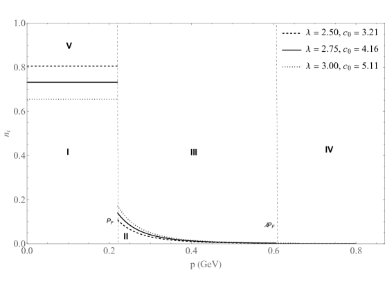
Figure 1: $n_{\mbox{\scriptsize CFG}}(\bm{p})$ as a a function of the magnitude of the 3-momentum. The different lines correspond to extremal variation of $\lambda$ and $c_{0}$. The labels for the regions I-V are explained in the text.

$n_{\mbox{\scriptsize CFG}}(\bm{p})$ is plotted in figure 1. It exhibits a depleted Fermi gas region and a correlated high-momentum tail. The dashed and dotted lines correspond to the maximum and minimum limits for the high momentum cut-off $\lambda$ and parameter $c_{0}$, with the central value represented by a straight line. Unlike the RFG model where the nucleon can be either “inside” or “outside” the nucleus, for the CFG model we can distinguish five regions. The initial nucleon can be in region I if $0\leq|\bm{p}|\leq p_{F}$, or in region II if $p_{F}\leq|\bm{p}|\leq\lambda p_{F}$. The final nucleon can be in three possible regions. Region III corresponds to $p_{F}\leq|\bm{p^{\prime}}|\leq\lambda p_{F}$, region IV to $\lambda p_{F}\leq|\bm{p^{\prime}}|$, and region V to $0\leq|\bm{p^{\prime}}|\leq p_{F}$. In the formal limit $\lambda\to 1$, regions II, III, and V vanish and we are left with the RFG model. Since $\lambda\approx 2.75\pm 0.25$, this limit is never obtained in practice.

3 Implementation of the CFG model

Using the properly normalized expression for $n_{\mbox{\scriptsize CFG}}(\bm{p})$ in equations (21) and (7), we derive explicit expressions for $W_{i}$. These will be more complicated than the ones for the RFG model since the momentum distribution is more complicated. Here we outline the implementation with detailed expressions relegated to the appendices.

3.1 Calculation of the nuclear tensor

As discussed above, the initial nucleon can be in regions I or II, while the final nucleon can be in regions III, IV or V. Thus we have six possible transitions: I$\to$ III, I$\to$ IV, I$\to$ V, II$\to$ III, II$\to$ IV, II$\to$ V. For each of these transitions we calculate $W_{i}$ separately and find the cross section. The total cross section will be the sum of these possible cases. Since the momentum dependence in $n_{\mbox{\scriptsize CFG}}$ is either a constant or inversely proportional to the fourth power of the three-momentum, these six transitions depend on four possible combinations of initial and final momentum dependencies. Thus the five $W_{i}$ depend on the five $H_{i}$ via the seven functions $a_{j}$ as in the RFG model, but we need to define four sets of such functions. Each set in turn depends on three master $b$ integrals over the initial energy $E_{\bm{p}}$, analogous to the ones in the RFG case. The detailed expressions appear in appendix B.

To give a flavor of these expressions, assume that for a given value $\bm{p}$, $\bm{q}$ and $\omega$, there is a transition from region II$\to$ III. The energy-conserving delta function in equation (8) requires that $\epsilon_{\bm{p}}-\epsilon^{\prime}_{\bm{p}+\bm{q}}+q^{0}=0$ or $E_{\bm{p}+\bm{q}}=E_{\bf p}+\omega_{\mbox{\scriptsize eff}}$, where $\omega_{\mbox{\scriptsize eff}}=\omega-\epsilon_{b}$. This implies $|\bm{p}^{\prime}|^{-4}=|\bm{p}+\bm{q}|^{-4}=(E_{{\bf p}+{\bf q}}^{2}-m^{2}_{N})^{-2}=\left[(E_{\bf p}+\omega_{\mbox{\scriptsize eff}})^{2}-m_{N}^{2}\right]^{-2}$. Similarly for the initial state $|\bm{p}|^{-4}=\left(E_{{\bf p}}^{2}-m^{2}_{N}\right)^{-2}$. Thus the integrals over the function $f({\bm{p}},q^{0},\bm{q})$ contain $\alpha_{1}\left(E_{{\bf p}}^{2}-m^{2}_{N}\right)^{-2}\left(1-\alpha_{1}\left[(E_{\bf p}+\omega_{\mbox{\scriptsize eff}})^{2}-m_{N}^{2}\right]^{-2}\right)$. The energy-conserving delta function is used to fix the angle between $\bm{p}$ and $\bm{q}$ and the integral over $d^{3}p$ can be replaced by an integral over $E_{p}$. Similar considerations can be applied to other transitions. The explicit expressions are listed in appendix B. The limits of integration are different for each of the six transitions and we discuss them next.

3.2 Limits of integration

The definite integrals over $E_{\bm{p}}$ have the limits $E_{\mbox{\scriptsize low}}\leq E_{\bm{p}}\leq E_{\mbox{\scriptsize high}}$. The values of $E_{\mbox{\scriptsize low}}$ and $E_{\mbox{\scriptsize high}}$ are different for each of the six possible transitions.

Define $\omega=q^{0},\omega_{\mbox{\scriptsize eff}}=\omega-\epsilon_{b},c=-\omega_{\mbox{\scriptsize eff}}/|\bm{q}|$, $d=-(\omega_{\mbox{\scriptsize eff}}^{2}-|\bm{q}|^{2})/(2|\bm{q}|m_{N})$, $E_{F}^{\lambda}=\sqrt{m_{N}^{2}+\left(\lambda p_{F}\right)^{2}}$. One condition arises from the constraints on the scattering angle. The scattering angle $\theta_{\bm{pq}}$ satisfies $-1\leq\cos\theta_{\bm{pq}}\leq 1$, or

$$-1\leq\cos\theta_{\bm{pq}}\leq 1\quad\Rightarrow\quad-1\leq\frac{\omega_{\rm eff}^{2}-|\bm{q}|^{2}+2\omega_{\rm eff}E_{\bm{p}}}{2|\bm{q}|\sqrt{E_{\bm{p}}^{2}-m_{N}^{2}}}\leq 1,$$ (23)

The latter condition can be expressed as

$$\left(\frac{E_{\bm{p}}}{m_{N}}-\frac{cd+\sqrt{1-c^{2}+d^{2}}}{1-c^{2}}\right)\left(\frac{E_{\bm{p}}}{m_{N}}-\frac{cd-\sqrt{1-c^{2}+d^{2}}}{1-c^{2}}\right)\geq 0\,.$$ (24)

Defining $\Delta\equiv m_{N}(cd+\sqrt{1-c^{2}+d^{2}})/(1-c^{2})$ this implies $\Delta\leq E_{\bm{p}}$. This condition holds for all regions.

For region I we have by definition $0\leq E_{\bm{p}}\leq E_{F}$. For region II we have by definition $E_{F}\leq E_{\bm{p}}\leq E_{F}^{\lambda}$. Also, the final state has energy of $E_{\bm{p}}+\omega_{\mbox{\scriptsize eff}}$. We now apply these conditions to each transition.

I$\to$ III:

Since $E_{\bm{p}}+\omega_{\mbox{\scriptsize eff}}\in$ III, $E_{F}\leq E_{\bm{p}}+\omega_{\mbox{\scriptsize eff}}\leq E_{F}^{\lambda}\Rightarrow E_{F}-\omega_{\mbox{\scriptsize eff}}\leq E_{\bm{p}}\leq E_{F}^{\lambda}-\omega_{\mbox{\scriptsize eff}}$. Together with the conditions $\Delta\leq E_{\bm{p}}$, $0\leq E_{\bm{p}}\leq E_{F}$ we have

$$\mbox{I$\to$ III:}\quad E_{\mbox{\scriptsize low}}=\mbox{max}\left(\Delta,E_{F}-\omega_{\mbox{\scriptsize eff}}\right),\quad E_{\mbox{\scriptsize high}}=\mbox{min}\left(E_{F},E_{F}^{\lambda}-\omega_{\mbox{\scriptsize eff}}\right).$$ (25)

I$\to$ IV:

Since $E_{\bm{p}}+\omega_{\mbox{\scriptsize eff}}\in$ V, $E_{F}^{\lambda}\leq E_{\bm{p}}+\omega_{\mbox{\scriptsize eff}}\Rightarrow E_{F}^{\lambda}-\omega_{\mbox{\scriptsize eff}}\leq E_{\bm{p}}$. Together with the conditions $\Delta\leq E_{\bm{p}}$, $0\leq E_{\bm{p}}\leq E_{F}$ we have

$$\mbox{I$\to$ IV:}\quad E_{\mbox{\scriptsize low}}=\mbox{max}\left(\Delta,E_{F}^{\lambda}-\omega_{\mbox{\scriptsize eff}}\right),\quad E_{\mbox{\scriptsize high}}=E_{F}.$$ (26)

I$\to$ V:

Since $E_{\bm{p}}+\omega_{\mbox{\scriptsize eff}}\in$ V, $0\leq E_{\bm{p}}+\omega_{\mbox{\scriptsize eff}}\leq E_{F}\Rightarrow-\omega_{\mbox{\scriptsize eff}}\leq E_{\bm{p}},E_{\bm{p}}\leq E_{F}-\omega_{\mbox{\scriptsize eff}}$. Together with the conditions $\Delta\leq E_{\bm{p}}$, $0\leq E_{\bm{p}}\leq E_{F}$ we have

$$\mbox{I$\to$ V:}\quad E_{\mbox{\scriptsize low}}=\mbox{max}\left(\Delta,-\omega_{\mbox{\scriptsize eff}}\right),\quad E_{\mbox{\scriptsize high}}=\mbox{min}\left(E_{F},E_{F}-\omega_{\mbox{\scriptsize eff}}\right).$$ (27)

II$\to$ III:

Since $E_{\bm{p}}+\omega_{\mbox{\scriptsize eff}}\in$ III, $E_{F}\leq E_{\bm{p}}+\omega_{\mbox{\scriptsize eff}}\leq E_{F}^{\lambda}\Rightarrow E_{F}-\omega_{\mbox{\scriptsize eff}}\leq E_{\bm{p}}\leq E_{F}^{\lambda}-\omega_{\mbox{\scriptsize eff}}$. Together with the conditions $\Delta\leq E_{\bm{p}}$, $E_{F}\leq E_{\bm{p}}\leq E_{F}^{\lambda}$ we have

$$\mbox{II$\to$ III:}\quad E_{\mbox{\scriptsize low}}=\mbox{max}\left(\Delta,E_{F},E_{F}-\omega_{\mbox{\scriptsize eff}}\right),\quad E_{\mbox{\scriptsize high}}=\mbox{min}\left(E_{F}^{\lambda},E_{F}^{\lambda}-\omega_{\mbox{\scriptsize eff}}\right).$$ (28)

II$\to$ IV:

Since $E_{\bm{p}}+\omega_{\mbox{\scriptsize eff}}\in$ IV, $E_{F}^{\lambda}\leq E_{\bm{p}}+\omega_{\mbox{\scriptsize eff}}\Rightarrow E_{F}^{\lambda}-\omega_{\mbox{\scriptsize eff}}\leq E_{\bm{p}}$. Together with the conditions $\Delta\leq E_{\bm{p}}$, $E_{F}\leq E_{\bm{p}}\leq E_{F}^{\lambda}$ we have

$$\mbox{II$\to$ IV:}\quad E_{\mbox{\scriptsize low}}=\mbox{max}\left(\Delta,E_{F},E_{F}^{\lambda}-\omega_{\mbox{\scriptsize eff}}\right),\quad E_{\mbox{\scriptsize high}}=E_{F}^{\lambda}.$$ (29)

II$\to$ V:

Since $E_{\bm{p}}+\omega_{\mbox{\scriptsize eff}}\in$ V, $0\leq E_{\bm{p}}+\omega_{\mbox{\scriptsize eff}}\leq E_{F}\Rightarrow-\omega_{\mbox{\scriptsize eff}}\leq E_{\bm{p}},E_{\bm{p}}\leq E_{F}-\omega_{\mbox{\scriptsize eff}}$. Together with the conditions $\Delta\leq E_{\bm{p}}$, $E_{F}\leq E_{\bm{p}}\leq E_{F}^{\lambda}$ we have

$$\mbox{II$\to$ V:}\quad E_{\mbox{\scriptsize low}}=\mbox{max}\left(\Delta,E_{F},-\omega_{\mbox{\scriptsize eff}}\right),\quad E_{\mbox{\scriptsize high}}=\mbox{min}\left(E_{F}^{\lambda},E_{F}-\omega_{\mbox{\scriptsize eff}}\right).$$ (30)

3.3 Calculation of the cross section

For each possible transition we use the limits of integration from section (3.2) for the $a$ integrals from (B) in appendix B. Using equation (2.2) we combine those with the components of the nucleon tensor $H_{i}$ to obtain the final expression for $W_{i}$. To calculate the cross section we add all the possible transitions, namely,

$$d\sigma=d\sigma_{I\to III}+d\sigma_{I\to IV}+d\sigma_{I\to V}+d\sigma_{II\to III}+d\sigma_{II\to IV}+d\sigma_{II\to V}.$$ (31)

The limits of integration ensure that transitions that are not allowed kinematically do not contribute.

4 Results

Having derived analytical expressions for the cross section, we now compare them to data. We compare the predictions to electron-carbon data from [41, 42] and flux-averaged neutrino scattering data from the MiniBooNE experiment [15]. In the following we focus on the differences between the RFG and CFG models and different form factor parameterizations.

4.1 Electron scattering

We compare the predictions of the RFG and CFG models to electron-carbon scattering data. Since for both models the proton and neutron momentum distributions are independent, we add the cross sections for scattering off protons and neutrons separately. Recall that the distributions are normalized to $A/2$, where for carbon $A=12$.

The difference between the scattering on protons and neutrons arises from the different electromagnetic form factors of each nucleon. We compare two different electromagnetic form factor parameterizations, the commonly used BBBA [1] and the $z$-expansion based parameterization from [2], referred to as BHLT in the following. BHLT is our default parameterization. Details about these parameterizations appear in appendix C.

The electron-carbon scattering data is taken from the compilation in [41, 42]. There are 66 kinematical points corresponding to different values of the initial electron energy and final electron scattering angle. We present a few of them here and include more in appendix D.

Consider first a comparison of RFG and CFG models with the BHLT parameterization to carbon data with incident electron energy of 480 MeV and a scattering angle of $60^{\circ}$, see figure 2. In comparing RFG and CFG, we see that the $\omega$ values of the CFG data points extend beyond the RFG data points. These reflect the phase space limits for each model. For the RFG model the limits for $E_{\bm{p}}$ are $E_{\mbox{\scriptsize low}}=\mbox{max}\left(\Delta,E_{F}-\omega_{\mbox{\scriptsize eff}}\right)$ and $E_{\mbox{\scriptsize high}}=E_{F}$. For the considered kinematics, these translate to $0.031\,\mbox{GeV}\leq\omega\leq 0.196\,$GeV.

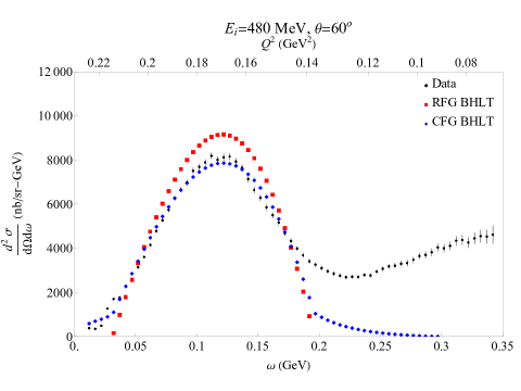
Figure 2: A comparison of RFG (red squares) and CFG (blue diamonds) models to carbon data. The incident electron energy is 480 MeV and the scattering angle is $60^{\circ}$. The error bars from the form factor uncertainties are smaller than the markers’ size of the $\mathcal{O}(10^{1})$ nb/sr-GeV.

To better understand the CFG case, we show the cross section for this kinematics for each of the six possible transitions in figure 3. The cross section is dominated by transitions from region I to region III. The shape of the cross section for such transitions is analogous to that of the RFG model. The “tail” for larger values of $\omega$ is generated by transitions from region I and II to region IV. Only the transition from region II to region IV has values of $\omega$ larger than the RFG case, where $\omega$ can be as large as 0.298 GeV for this kinematics. The “tail” for smaller values of $\omega$ is mostly generated by transitions from region II to region III. The transition from region II to V gives a very small contribution, a few percent of the total cross section in the small-$\omega$ region. The transition from region I to V does not contribute for this kinematics. Notice also that different transitions can have the same value of $\omega$ since they will originate from different values of $E_{\bm{p}}$.

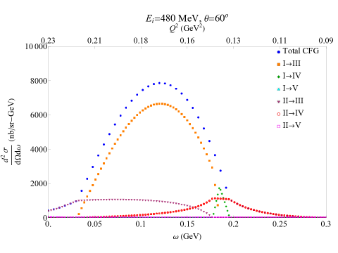
Figure 3: The contributions to the CFG model cross section by transitions. The incident electron energy is 480 MeV and the scattering angle is $60^{\circ}$.

In plotting the CFG predictions we use the central values of the model parameters, $\lambda$ and $c_{0}$. Varying of the model parameters results in broadening of the scattering cross-section prediction. We illustrate by the band in figure 4 for the case of an incoming electron energy of 480 MeV and scattering angle of $60^{\circ}$. We again use the BHLT form factor parametrization. Comparing to figure 2, the variation of the CFG parameters is smaller than the difference between the RFG and CFG models.

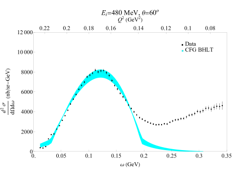
Figure 4: A comparison between the carbon data and CFG nuclear model using the BHLT parametrization for values of $\lambda$ and $c_{0}$ in the range [2.5, 3.0] and [3.21, 5.11] respectively.

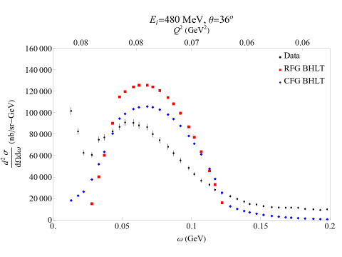
Figure 5: A comparison of RFG (red squares) and CFG (blue diamonds) models to carbon data. The incident electron energy is 480 MeV and the scattering angle is $36^{\circ}$. The error bars for the RFG and CFG are of the $\mathcal{O}(10^{2})$ nb/sr-GeV, which remain invisible due to the size of the markers.

For carbon data with incident electron energy of 480 MeV and a scattering angle of $60^{\circ}$, the CFG model fits the data better than the RFG model. The same is true if the change the angle the scattering angle to $36^{\circ}$, but the overall fit is worse, see figure 5.

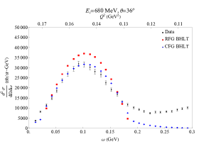
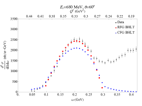
Figure 6: A comparison of RFG (red squares) and CFG (blue diamonds) models to carbon data. The incident electron energy is 680 MeV. Left: Scattering angle of $36^{\circ}$ Left: Scattering angle of $60^{\circ}$. The error bars for the RFG and CFG are of the $\mathcal{O}(10^{2})$ nb/sr-GeV for $36^{\circ}$ and $\mathcal{O}(10^{1})$ nb/sr-GeV for $60^{\circ}$

In figure 6 we compare the RFG and CFG models to carbon data with incident electron energy of 680 MeV and a scattering angle of $36^{\circ}$ (left) and $60^{\circ}$ (right). For this energy the CFG model fits the data better for $36^{\circ}$, while the RFG model fits the data better for $60^{\circ}$.

Finally, we compare the RFG and CFG models to carbon data with incident electron energy of 240 MeV and a scattering angle of $36^{\circ}$ (left) and $60^{\circ}$ (right), see figure 7. Neither of the models fits the data very well.

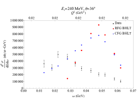
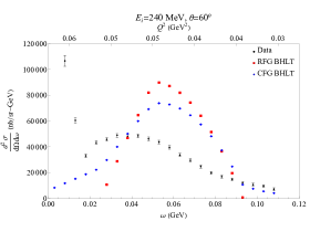
Figure 7: A comparison of RFG (red squares) and CFG (blue diamonds) models to carbon data. The incident electron energy is 240 MeV. Left: Scattering angle of $36^{\circ}$ Right: Scattering angle of $60^{\circ}$.The error bars for the RFG and CFG are of the $\mathcal{O}(10^{2})$ nb/sr-GeV with the error being larger for $36^{\circ}$ compared to $60^{\circ}$

A different interesting physics question is the separation of nuclear effects, captured by the nuclear model, and nucleon effects, captured by the form factors. To address this question, we compare the RFG and CFG models to data with two different parameterizations: BBBA [1] and BHLT [2]. In figure 8 we compare each nuclear model using the different parameterizations to carbon data with incident electron energy of 480 MeV and a scattering angle of $60^{\circ}$. It is clear that the differences between different parameterizations are small compared to the differences between the nuclear models themselves. For example, the maximum value of the differential cross section is at $\omega=0.122$ GeV. In units of nb/sr-GeV we have for the RFG model $9159\pm 37$ (BHLT) and $8968\pm 146$ (BBBA), while for the CFG model we have $7861\pm 32$ (BHLT), $7698\pm 125$ (BBBA).

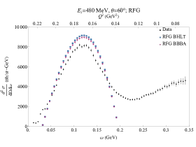
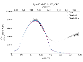
Figure 8: A comparison of RFG (left) and CFG (right) models to carbon data with the BBBA and $z$-expansion based parameterizations. The incident electron energy is 480 MeV and the scattering angle is $60^{\circ}$.

4.2 Neutrino scattering

In comparing the CFG model to data, neutrino scattering differs from electron scattering in two important aspects. First, the interaction involves also the axial current apart from the vector current. This requires us to consider five different scalar components of the nuclear tensor: $W_{1},\dots,W_{5}$. For the CFG model the extension is clear. We only need to specify two new form factors, $F_{A}$ and $F_{P}$ that appear in equation (2.1). Second, since the incident neutrino energy is not fixed, we need to average over the neutrino flux in order to compare to data.

Similar to the electromagnetic form factors $F_{1}$ and $F_{2}$, we consider several parameterizations for $F_{A}$. These can be divided to two classes. The first is the historical “dipole” model $F_{A}^{\rm dipole}(q^{2})=F_{A}(0)/{\left[1-{q^{2}/(m_{A}^{\rm dipole})^{2}}\right]^{2}}$ where $F_{A}(0)$ is measured in beta decay [43], and $m_{A}^{\rm dipole}$ is a free parameter. In the MiniBooNE analysis [15], $m_{A}^{\rm dipole}=1.35\pm 0.17$ GeV was obtained, while in the so called “BBBA07” parameterization [44], $m_{A}^{\rm dipole}=1.014\pm 0.014$ was obtained.

The second class are the $z$-expansion based parameterizations. These are more flexible and do not introduce an a priori functional form. For the axial form factor the method was pioneered in 2011 [16]. Since then it has been used in the literature to to extract the axial form factor using scattering data and Lattice QCD. In the following we list extractions that give the $z$-expansion coefficients and their uncertainties. In 2016 the axial form factor was extracted from neutrino-deuteron scattering data [34]. In 2023 it was extracted from antineutrino-proton scattering by the MINERvA experiment [35].

Recently, several lattice QCD $z$-expansion based parameterizations of the axial form factor that give the coefficients and their uncertainties became available. These are by the RQCD in 2020 [36], NME collaboration in 2021 [37], the Mainz group in 2022 [38], and in 2023 by the PNDME collaboration [39] and the ETMC collaboration [40].

In appendix C we plot the axial form factor from these various parameterizations. Similar plots are available in [45]. These plots suggest that [34] and [38] represent two extremes of possible parameterizations of $F_{A}$, with other parameterizations lying in between them. In the following we refer to [34] as “MBGH” and [38] as “Mainz22”, and use them to illustrate the possible range of axial form factor uncertainty.

Effects from $F_{P}$ are suppressed by $m_{\ell}^{2}/m_{T}^{2}$, see equations (2.1) and (2). Because of that, we use the pion-pole approximation $F_{P}(q^{2})\approx 2m_{N}^{2}F_{A}(q^{2})/(m_{\pi}^{2}-q^{2})$. There are extractions of $F_{P}$ from Lattice QCD in the references above and one could potentially use them instead.

4.2.1 Neutrino cross-section before flux averaging

Before comparing the CFG model predictions to MiniBooNE data, let us consider the hypothetical case of a fixed neutrino energy. Neutrino scattering experiments typically have a distribution of energies. We choose a neutrino energy of $E_{\nu}=1$ GeV, around the peak energy of the MiniBooNE neutrino flux.

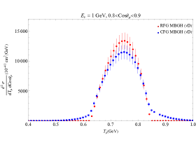
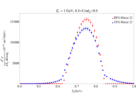
Figure 9: A comparison between RFG (red circles) and CFG (blue squares) model double differential scattering cross-section using fixed incoming neutrino energy of $1000$ MeV as a function of the outgoing muon kinetic energy scattering at an angle of $\cos\theta_{\mu}=0.85$ Left: MBGH axial form factor and Right: Mainz22 axial form factor.

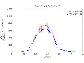
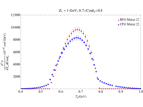
Figure 10: A comparison between RFG (red circles) and CFG (blue squares) model double differential scattering cross-section using fixed incoming neutrino energy of $1000$ MeV as a function of the outgoing muon kinetic energy scattering at an angle of $\cos\theta_{\mu}=0.75$ Left: MBGH axial form factor and Right: Mainz22 axial form factor.

We compare the RFG and CFG model predictions for the differential cross section of scattering of a 1 GeV neutrino off carbon for $\cos\theta_{\mu}=0.85$ (figure 9) and $\cos\theta_{\mu}=0.75$ (figure 10). The predictions are plotted as a function of the muon kinetic energy $T_{\mu}=E_{\mu}-m_{\mu}$. For a fixed neutrino energy the relation between $\omega$ and $T_{\mu}$ is $T_{\mu}=E_{\nu}-m_{\mu}-\omega$. We use BHLT parameterization for the vector form factors and compare MBGH and Mainz22 for the axial form factor. At the “tail” region of high or low $T_{\mu}$ we can clearly distinguish between the RFG and CFG model predictions, independent of the axial form factor parameterization. At the “peak” region we can distinguish between RFG and CFG model predictions only for the Mainz22 parameterization. For the MBGH parameterization the uncertainties overlap between the two nuclear models.

4.2.2 Neutrino cross section after flux averaging

We now consider predictions where the neutrino cross section is convoluted with the neutrino flux distribution. In particular we have [17]

$$\frac{d\sigma_{\rm carbon,per\,nucleon,avg.}}{dE_{\ell}d\cos\theta_{\ell}}=\int dE_{\nu}\,f(E_{\nu})\,\frac{d\sigma_{\rm carbon,per\,nucleon}}{dE_{\ell}d\cos\theta_{\ell}}.$$ (32)

We first consider a fixed axial form factor parameterization and vary the nuclear models. In figures 11 and 12 we show the comparison of the RFG and CFG model to the MiniBooNE data for two different bins of $\cos\theta$ and different values of $T_{\mu}=E_{\mu}-m_{\mu}$. Unlike the scattering of neutrinos with fixed energy, for the flux averaged cross section we cannot distinguish between the RFG and CFG models. The reason is that the averaging over the flux “adds” several cross sections that peak at different values of $\omega$ ,“smearing” the tails of the cross section. This conclusion is true for either choice of the two $F_{A}$ parameterizations of MBGH and Mainz 22. We also see that the Mainz22 $F_{A}$ fits the data much better than MBGH. This is not surprising considering that the Mainz22 $F_{A}$ largely overlaps with the dipole $F_{A}$ with $m_{A}^{\rm dipole}$ extracted by MiniBooNE [15] assuming the RFG model, see the left hand side of figure 16.

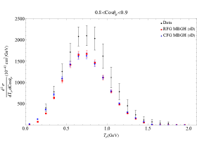
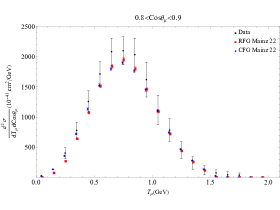
Figure 11: A comparison of RFG (red squares) and CFG (blue diamonds) models to flux averaged neutrino - carbon scattering data as a function of the outgoing muon kinetic energy scattering at an angle of $0.8<\cos\theta_{\mu}<0.9$ using Left: MBGH axial form factor Right: Mainz 22 for the axial form factor (BHLT parametrization is used for the electric and magnetic form factors in both cases).

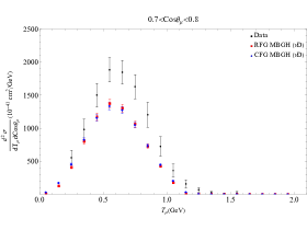
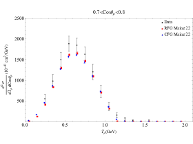
Figure 12: A comparison of RFG (red squares) and CFG (blue diamonds) models to flux averaged neutrino - carbon scattering data as a function of the outgoing muon kinetic energy scattering at an angle of $0.7<\cos\theta_{\mu}<0.8$ using Left: MBGH axial form factor Right: Mainz 22 for the axial form factor (BHLT parametrization is used for the electric and magnetic form factors in both cases).

This is a somewhat disappointing result. At least for the MiniBooNE data, we cannot distinguish between the two models. It would be interesting to see if this phenomena still persists in less inclusive observable, e.g. semi-inclusive neutrino scattering.

Next we vary the axial form factor parameterization and consider a fixed nuclear model. In figures 13 and 14 we compare the effects of a wide range of $F_{A}$ parameterizations on the neutrino cross section for both RFG and CFG models. As expected from the right hand side of figure 16, there is almost a continuous “spread” from the $F_{A}$ parameterizations, for both nuclear models. We conclude that the axial form factor uncertainty is the dominant one.

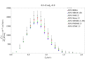
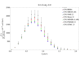
Figure 13: A comparison of BBBA, MBGH, NME 22, Mainz 22, MINERvA ($\bar{\nu}$H), PNDME 23 and ETMC 23 form factor parametrization to flux averaged neutrino - carbon scattering data as a function of the outgoing muon kinetic energy scattering at an angle of $0.8<\cos\theta_{\mu}<0.9$ using Left: RFG model Right: CFG model (BHLT parametrization is used for the electric and magnetic form factors in all the cases except for BBBA).

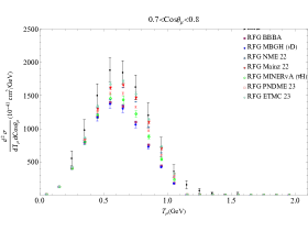
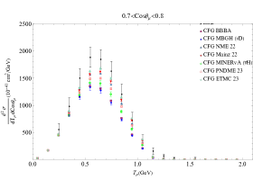
Figure 14: A comparison of BBBA, MBGH, NME 22, Mainz 22, MINERva ($\bar{\nu}$H), PNDME 23 and ETMC 23 form factor parametrization to flux averaged neutrino - carbon scattering data as a function of the outgoing muon kinetic energy scattering at an angle of $0.7<\cos\theta_{\mu}<0.8$ using Left: RFG model Right: CFG model (BHLT parametrization is used for the electric and magnetic form factors all the cases except NME and BBBA)

5 Summary and outlook

The neutrino research program in the coming decades will require improved precision. A major source of uncertainty is the interaction of neutrinos with nuclei that serve as the target of many such experiments. Broadly speaking, this interaction often depends, e.g., for CCQE, on the combination of “nucleon physics”, expressed by form factors, and “nuclear physics”, expressed by a nuclear model. It is important to get a good handle on both.

In this paper we presented a fully analytic implementation of the Correlated Fermi Gas (CFG) Model for CCQE electron-nucleus and neutrino-nucleus scattering. We then use this implementation to compare separately form factors and nuclear model effects for both electron-carbon and neutrino-carbon scattering data.

For CCQE in the CFG model the initial nucleon can be in two possible momentum regions that we label I and II, and the final nucleon can be in three momentum regions that we label III, IV, and V, see figure 1. The total cross section is given as a sum of the possible six transitions, see equation (31). The differential cross section for each transition is expressed by the component of the nuclear tensor $W_{i}$, see equations (2) and (3). $W_{i}$ for each possible transition is expressed as a sum of products of a single-nucleon tensor components and a phase space integrals $a_{1,\dots,7}$, see equation (2.2). The single-nucleon tensor components are given in equation (2.1). The phase space integrals for each transition are given in equation (B). They can be expressed by a smaller set of master integrals, see equation (B). The limits of the integrals are given in section 3.2. Combining all these elements gives an explicit analytical expression for the differential cross section.

Using these analytical expressions, we compared the CFG model prediction in section 4 to electron-carbon data and neutrino scattering data from the MiniBooNE experiment. We focused on the differences between the RFG and CFG models and the effects of different form factor parameterizations.

In section 4.1 we compared the predictions of the RFG and CFG models to electron-carbon scattering data. We have used the BHLT [2] parameterization of the vector form factors as our default. In all cases one can clearly distinguish the two models, where the CFG model has a “tail” in small and large value of $\omega$. At the peak region of the differential cross section, the CFG model prediction is smaller than the RFG model prediction. The agreement with the data varies depending on the electron energy and scattering angle, see figures 2-7. We also found that the differences between BBBA [1] and BHLT parameterizations of the electromagnetic form factors were small compared to the differences between the nuclear models, see figure 8.

In section 4.2 we compared the predictions of the RFG and CFG models to neutrino-carbon scattering. The nucleon axial form factor plays an important role in this interaction. We used two “extremes” of possible parameterizations of $F_{A}$, MBGH [34] and Mainz22 [38], with other parameterizations lying in between them.

First, we considered the hypothetical case of the fixed neutrino energy, $1$ GeV, around the peak of the MiniBooNE neutrino energy flux. At the “tail” regions we could clearly distinguish between the RFG and CFG models, independent of the axial form factor parameterization. At the “peak” region we could distinguish between RFG and CFG model predictions only for the Mainz22 parameterization, and not for the MBGH parameterization, see figures 9 and 10.

Next, we compared to MiniBooNE data the flux averaged neutrino cross section. Unlike the scattering of neutrinos with fixed energy, we could not distinguish between the RFG and CFG models using either MBGH or Mainz22. This is a somewhat disappointing result. It would be interesting to see if this phenomena still persists in less inclusive observable, e.g. semi-inclusive neutrino scattering. For both models Mainz22 fits the data much better than MBGH. This is to be expected since Mainz22 $F_{A}$ largely overlaps with the dipole $F_{A}$ with $m_{A}^{\rm dipole}$ extracted by MiniBooNE [15] assuming the RFG model, see figure 16. Finally, we used the larger set of $F_{A}$ parameterizations that lay between MBGH or Mainz22 together with the RFG and CFG nuclear models. We found an almost continuous “spread” in the predictions generated using these $F_{A}$ parameterizations for both RFG and CFG nuclear models. This highlights the need to get a smaller and more consistent uncertainty for $F_{A}$.

We hope that the analytic implementation of the CFG model we presented can be easily included in neutrino event generators. The analytic implementation can be adapted in the future to less inclusive observables. For example, one can consider the kinematics of the final state nucleon by not integrating over the final state nucleon in equation (4). In the future it would be also interesting to combine the CFG model with other effects such as final state interactions (FSI).

Acknowledgements We thank Jameson Tockstein, Joseph Wieske, and Malik Swain for collaboration in earlier stages of the project. We also thank Adi Ashkenazi, Or Hen, Kevin McFarland, and Eliezer Piasetzky for useful discussions. This work was supported by the U.S. Department of Energy grant DE-SC0007983 (S.C., G.P.) and the National Science Foundation under grant no. PHY-2310627 (B.B.).

Appendix A Values of parameters

We present in table 1 the values of the parameters used in this paper and the reference to each value.

Table 1: Values of parameters

Name	Parameter	Value and unit	Reference
EM fine structure constant	$\alpha$	$1/137.036$	[43]
Proton mass	$m_{p}$	938.272 MeV	[43]
Neutron mass	$m_{n}$	939.565 MeV	[43]
Proton magnetic moment	$\mu_{p}$	2.79285	[43]
Neutron magnetic moment	$\mu_{n}$	$-1.91304$	[43]
Vector mass	$m_{V}$	843 MeV	[46]
Pion mass	$m_{\pi}$	139.57 MeV	[43]
Carbon binding energy	$\epsilon_{b}$	25 MeV	[18]
Carbon Fermi momentum	$p_{F}$	220 MeV	[15]
CFG model parameter	$\lambda$	$2.75\pm 0.25$	[27]
CFG model parameter	$c_{0}$	$4.16\pm 0.95$	[27]

Appendix B Appendix: Expressions for $a$ and $b$ functions

Following [16] we find the expressions for $a_{i}$s to be as follows:

$$a_{1} = \int d^{3}{\bf p}f({\bf p},q^{0},{\bf q})~{},~{}~{}$$ (33)

$$a_{2} = \int d^{3}{\bf p}f({\bf p},q^{0},{\bf q})~{}\dfrac{|{\bf p}|^{2}}{m_{N}^{2}}~{}=~{}\int d^{3}{\bf p}f({\bf p},q^{0},{\bf q})~{}\dfrac{E_{\bf p}^{2}-m^{2}_{N}}{m_{N}^{2}}~{},~{}~{}$$ (34)

$$a_{3} = \int d^{3}{\bf p}f({\bf p},q^{0},{\bf q})~{}\dfrac{p^{2}_{z}}{m_{N}^{2}}~{}=~{}\int d^{3}{\bf p}f({\bf p},q^{0},{\bf q})~{}\cos^{2}\theta_{{\bf p}{\bf q}}~{}\dfrac{E_{\bf p}^{2}-m^{2}_{N}}{m_{N}^{2}}~{},~{}~{}$$ (35)

$$a_{4} = \int d^{3}{\bf p}f({\bf p},q^{0},{\bf q})~{}\dfrac{\epsilon_{\bf p}^{2}}{m_{N}^{2}}~{}=~{}\int d^{3}{\bf p}f({\bf p},q^{0},{\bf q})~{}\dfrac{(E_{\bf p}-\epsilon_{b})^{2}}{m_{N}^{2}}~{},~{}~{}$$ (36)

$$a_{5} = \int d^{3}{\bf p}f({\bf p},q^{0},{\bf q})~{}\dfrac{\epsilon_{\bf p}p_{z}}{m_{N}^{2}}~{}=~{}\int d^{3}{\bf p}f({\bf p},q^{0},{\bf q})~{}\cos\theta_{{\bf p}{\bf q}}~{}\dfrac{(E_{\bf p}-\epsilon_{b})|{\bf p}|}{m_{N}^{2}}~{},~{}~{}$$ (37)

$$a_{6} = \int d^{3}{\bf p}f({\bf p},q^{0},{\bf q})~{}\dfrac{p_{z}}{m_{N}}~{}=~{}\int d^{3}{\bf p}f({\bf p},q^{0},{\bf q})~{}\cos\theta_{{\bf p}{\bf q}}~{}\dfrac{|{\bf p}|}{m_{N}}~{},~{}~{}$$ (38)

$$a_{7} = \int d^{3}{\bf p}f({\bf p},q^{0},{\bf q})~{}\dfrac{\epsilon_{\bf p}}{m_{N}}~{}=~{}\int d^{3}{\bf p}f({\bf p},q^{0},{\bf q})~{}\dfrac{(E_{\bf p}-\epsilon_{b})}{m_{N}}~{},~{}~{}$$ (39)

where $\epsilon_{\bf p}~{}=~{}E_{\bf p}-\epsilon_{b}~{},~{}\epsilon^{\prime}_{{\bf p}^{\prime}}~{}=~{}E_{{\bf p}^{\prime}}~{},~{}E_{{\bf p}}^{2}~{}=~{}{\bf p}^{2}+m_{N}^{2}~{}.~{}$ The integrals have the generic form

$$\int d^{3}{\bf p}f({\bf p},q^{0},{\bf q})X({\bf p}) = \dfrac{m_{T}V}{4\pi^{2}}\int d^{3}{\bf p}~{}n_{i}({\bf p})(1-n_{f}({\bf p}+{\bf q}))\dfrac{\delta(\epsilon_{\bf p}-\epsilon^{\prime}_{{\bf p}+{\bf q}}+q^{0})}{\epsilon_{{\bf p}}\epsilon^{\prime}_{{\bf p}+{\bf q}}}X({\bf p})~{},~{}~{}~{}~{}$$ (40)

$$= \dfrac{m_{T}V}{4\pi^{2}}\int\dfrac{d^{3}{\bf p}}{(E_{\bf p}-\epsilon_{b})|{\bf p}||{\bf q}|}~{}n_{i}({\bf p})(1-n_{f}({\bf p}+{\bf q}))~{}~{}~{}$$

$$\hskip 72.26999pt\times~{}\delta\left(\cos\theta_{{\bf p}{\bf q}}-\dfrac{\omega^{2}_{\rm eff}-|{\bf q}|^{2}+2\omega_{\rm eff}E_{{\bf p}}}{2|{\bf p}||{\bf q}|}\right)X({\bf p})~{},~{}~{}$$

where $X({\bf p})$ is a function of $\bm{p}$ and we have used

$$\delta(\epsilon_{\bf p}-\epsilon^{\prime}_{{\bf p}+{\bf q}}+q^{0})~{}=~{}\dfrac{E_{{\bf p}+{\bf q}}}{|{\bf p}||{\bf q}|}~{}\delta\left(\cos\theta_{{\bf p}{\bf q}}-\dfrac{\omega^{2}_{\rm eff}-|{\bf q}|^{2}+2\omega_{\rm eff}E_{{\bf p}}}{2|{\bf p}||{\bf q}|}\right)~{}.~{}~{}$$ (41)

The above delta function also enforces the condition $E_{{\bf p}+{\bf q}}=E_{\bf p}+\omega_{\rm eff}$. For the CFG model $n_{i,f}$ depend on either a constant or $|\bm{p}+\bm{q}|^{-4}$ or $|\bm{p}|^{-4}$. The integration over the delta function simply enforces $|{\bf q}|^{2}+2{\bf p}\cdot{\bf q}=\omega_{\rm eff}^{2}+2\omega_{\rm eff}E_{\bf p}$ giving $|\bm{p}+\bm{q}|^{-4}=\left[(E_{\bf p}+\omega_{\mbox{\scriptsize eff}})^{2}-m_{N}^{2}\right]^{-2}$ and $|\bm{p}|^{-4}=\left(E_{{\bf p}}^{2}-m^{2}_{N}\right)^{-2}$.

Let $B(E_{\bf p})$ be the expression for $n_{i}({\bf p})(1-n_{f}({\bf p}+{\bf q}))$ after the integration over the delta function. For each of the possible six transitions we have

$$B({\rm I}\to{\rm III}) = \alpha_{0}\left(1-\frac{\alpha_{1}}{[(E_{{\bf p}}+\omega_{\mbox{\scriptsize eff}})^{2}-m^{2}_{N}]^{2}}\right)~{},~{}~{}$$

$$B({\rm I}\to{\rm IV}) = \alpha_{0}~{},~{}~{}$$

$$B({\rm I}\to{\rm V}) = \alpha_{0}(1-\alpha_{0})~{},~{}~{}$$

$$B({\rm II}\to{\rm III}) = \frac{\alpha_{1}}{(E_{{\bf p}}^{2}-m^{2}_{N})^{2}}\left(1-\frac{\alpha_{1}}{[(E_{{\bf p}}+\omega_{\mbox{\scriptsize eff}}]^{2}-m^{2}_{N})^{2}}\right)~{},~{}~{}$$

$$B({\rm II}\to{\rm IV}) = \frac{\alpha_{1}}{(E_{{\bf p}}^{2}-m^{2}_{N})^{2}}~{},~{}~{}$$

$$B({\rm II}\to{\rm V}) = \frac{\alpha_{1}(1-\alpha_{0})}{(E_{{\bf p}}^{2}-m^{2}_{N})^{2}}~{}.~{}~{}$$ (42)

These six transitions have only four independent functional forms.

Defining, as in the RFG model, $c=-\omega_{\rm eff}/|{\bf q}|$ and $d=-(\omega_{\rm eff}^{2}-|{\bf q}|^{2})/(2|{\bf q}|m_{N})$ and integrating over the delta function gives

$$\cos\theta_{{\bf p}{\bf q}} \to \dfrac{\omega^{2}_{\rm eff}-|{\bf q}|^{2}+2\omega_{\rm eff}E_{{\bf p}}}{2|{\bf p}||{\bf q}|}=-\dfrac{m_{N}d+E_{\bf p}c}{|{\bf p}|}~{},~{}~{}$$

$$\cos^{2}\theta_{{\bf p}{\bf q}} \to \left(\dfrac{\omega^{2}_{\rm eff}-|{\bf q}|^{2}+2\omega_{\rm eff}E_{{\bf p}}}{2|{\bf p}||{\bf q}|}\right)^{2}=\left(\dfrac{m_{N}d+E_{\bf p}c}{|{\bf p}|}\right)^{2}=\dfrac{E_{\bf p}^{2}c^{2}+2m_{N}E_{\bf p}cd+m_{N}^{2}d^{2}}{E_{\bf p}^{2}-m_{N}^{2}}.~{}~{}~{}$$ (43)

All together we have

$$a_{1} = \dfrac{m_{T}V}{2\pi|{\bf q}|}\int\dfrac{E_{\bf p}dE_{\bf p}}{(E_{\bf p}-\epsilon_{b})}~{}B(E_{\bf p})~{},~{}~{}$$

$$a_{2} = \dfrac{m_{T}V}{2\pi|{\bf q}|}\int\dfrac{E_{\bf p}dE_{\bf p}}{(E_{\bf p}-\epsilon_{b})}\left(\dfrac{E_{\bf p}^{2}}{m_{N}^{2}}-1\right)~{}B(E_{\bf p})~{},~{}~{}$$

$$a_{3} = \dfrac{m_{T}V}{2\pi|{\bf q}|}\int\dfrac{E_{\bf p}dE_{\bf p}}{(E_{\bf p}-\epsilon_{b})}\left(c^{2}\dfrac{E_{\bf p}^{2}}{m_{N}^{2}}+2cd\dfrac{E_{\bf p}}{m_{N}}+d^{2}\right)~{}B(E_{\bf p})~{},~{}~{}$$

$$a_{4} = \dfrac{m_{T}V}{2\pi|{\bf q}|}\int\dfrac{E_{\bf p}dE_{\bf p}}{(E_{\bf p}-\epsilon_{b})}\left(\dfrac{E_{\bf p}^{2}}{m_{N}^{2}}-2\dfrac{\epsilon_{b}}{m_{N}}\dfrac{E_{\bf p}}{m_{N}}+\dfrac{\epsilon_{b}^{2}}{m_{N}^{2}}\right)~{}B(E_{\bf p})~{},~{}~{}$$

$$a_{5} = \dfrac{m_{T}V}{2\pi|{\bf q}|}\int\dfrac{E_{\bf p}dE_{\bf p}}{(E_{\bf p}-\epsilon_{b})}\left(-~{}\dfrac{E_{\bf p}^{2}}{m_{N}^{2}}c+\left(\dfrac{\epsilon_{b}}{m_{N}}c-d\right)\dfrac{E_{\bf p}}{m_{N}}+\dfrac{\epsilon_{b}d}{m_{N}}\right)~{}B(E_{\bf p})~{},~{}~{}$$

$$a_{6} = \dfrac{m_{T}V}{2\pi|{\bf q}|}\int\dfrac{E_{\bf p}dE_{\bf p}}{(E_{\bf p}-\epsilon_{b})}\left(-~{}\dfrac{E_{\bf p}}{m_{N}}c-d\right)~{}B(E_{\bf p})~{},~{}~{}$$

$$a_{7} = \dfrac{m_{T}V}{2\pi|{\bf q}|}\int\dfrac{E_{\bf p}dE_{\bf p}}{(E_{\bf p}-\epsilon_{b})}\left(\dfrac{E_{\bf p}}{m_{N}}-\dfrac{\epsilon_{b}}{m_{N}}\right)~{}B(E_{\bf p})~{}.~{}~{}$$ (44)

These integrals can be expressed in terms of four sets of three master integrals

$$b_{1}^{j} = \dfrac{m_{T}V}{2\pi|{\bf q}|}\int\dfrac{E_{\bf p}dE_{\bf p}}{(E_{\bf p}-\epsilon_{b})}\left(\dfrac{E_{\bf p}}{m_{N}}\right)^{j}~{},~{}~{}$$

$$= \dfrac{m_{T}V}{2\pi|{\bf q}|m_{N}^{j}}\int\dfrac{E_{\bf p}^{j+1}dE_{\bf p}}{(E_{\bf p}-\epsilon_{b})}~{},~{}~{}$$

$$b_{2}^{j} = \dfrac{m_{T}V}{2\pi|{\bf q}|}\int\dfrac{E_{\bf p}dE_{\bf p}}{(E_{\bf p}-\epsilon_{b})(E^{2}_{\bf p}-m^{2}_{N})^{2}}\left(\dfrac{E_{\bf p}}{m_{N}}\right)^{j}~{},~{}~{}$$

$$= \dfrac{m_{T}V}{2\pi|{\bf q}|m_{N}^{j}}\int\dfrac{E_{\bf p}^{j+1}dE_{\bf p}}{(E_{\bf p}-\epsilon_{b})(E_{\bf p}^{2}-m^{2}_{N})^{2}}~{},~{}~{}$$

$$b_{3}^{j} = \dfrac{m_{T}V}{2\pi|{\bf q}|}\int\dfrac{E_{\bf p}dE_{\bf p}}{(E_{\bf p}-\epsilon_{b})((E_{\bf p}+\omega_{\mbox{\scriptsize eff}})^{2}-m^{2}_{N})^{2}}\left(\dfrac{E_{\bf p}}{m_{N}}\right)^{j}~{},~{}~{}$$

$$= \dfrac{m_{T}V}{2\pi|{\bf q}|m_{N}^{j}}\int\dfrac{E_{\bf p}^{j+1}dE_{\bf p}}{(E_{\bf p}-\epsilon_{b})((E_{\bf p}+\omega_{\mbox{\scriptsize eff}})^{2}-m^{2}_{N})^{2}}~{},~{}~{}$$

$$b_{4}^{j} = \dfrac{m_{T}V}{2\pi|{\bf q}|}\int\dfrac{E_{\bf p}dE_{\bf p}}{(E_{\bf p}-\epsilon_{b})(E_{\bf p}^{2}-m^{2}_{N})^{2}((E_{\bf p}+\omega_{\mbox{\scriptsize eff}})^{2}-m^{2}_{N})^{2}}\left(\dfrac{E_{\bf p}}{m_{N}}\right)^{j}~{},~{}~{}$$ (45)

$$= \dfrac{m_{T}V}{2\pi|{\bf q}|m_{N}^{j}}\int\dfrac{E_{\bf p}^{j+1}dE_{\bf p}}{(E_{\bf p}-\epsilon_{b})(E_{\bf p}^{2}-m^{2}_{N})^{2}((E_{\bf p}+\omega_{\mbox{\scriptsize eff}})^{2}-m^{2}_{N})^{2}},~{}~{}$$

where $j=0,1,2$. Note that $b_{1}^{j}$ is equal to $b_{j}$ as defined in Ref.[16] for the RFG case.
As an example, the integral $a_{3}$ for the six possible transitions are written in terms of $b_{1,2,3,4}^{j}$ as

$$a_{3}({\rm I}\to{\rm III}) = \alpha_{0}\Big{(}c^{2}b_{1}^{2}+2cdb_{1}^{1}+d^{2}b_{1}^{0}-\alpha_{1}(c^{2}b_{3}^{2}+2cdb_{3}^{1}+d^{2}b_{3}^{0})\Big{)}~{},~{}~{}$$

$$a_{3}({\rm I}\to{\rm IV}) = \alpha_{0}\Big{(}c^{2}b_{1}^{2}+2cdb_{1}^{1}+d^{2}b_{1}^{0}\Big{)}~{},~{}~{}$$

$$a_{3}({\rm I}\to{\rm V}) = \alpha_{0}(1-\alpha_{1})\Big{(}c^{2}b_{1}^{2}+2cdb_{1}^{1}+d^{2}b_{1}^{0}\Big{)}~{},~{}~{}$$

$$a_{3}({\rm II}\to{\rm III}) = \alpha_{1}\Big{(}c^{2}b_{2}^{2}+2cdb_{2}^{1}+d^{2}b_{2}^{0}-\alpha_{1}(c^{2}b_{4}^{2}+2cdb_{4}^{1}+d^{2}b_{4}^{0})\Big{)}~{},~{}~{}$$

$$a_{3}({\rm II}\to{\rm IV}) = \alpha_{1}\Big{(}c^{2}b_{2}^{2}+2cdb_{2}^{1}+d^{2}b_{2}^{0}\Big{)}~{},~{}~{}$$

$$a_{3}({\rm II}\to{\rm V}) = \alpha_{1}(1-\alpha_{0})\Big{(}c^{2}b_{2}^{2}+2cdb_{2}^{1}+d^{2}b_{2}^{0}\Big{)}~{}.~{}~{}$$ (46)

Similar expressions hold for other $a_{i}$. Similarly, as an example, one of the coefficients $W_{1}$ of the nuclear tensor which are functions of $b_{1,2,3,4}^{j}$ and the form factor for transition ${\rm I}\to{\rm V}$ is:

$$W_{1}^{{\rm I}\to{\rm V}} = \frac{3\pi A^{2}\alpha_{0}(1-\alpha_{0})(m_{N}-\epsilon_{b})}{32m_{N}^{2}p_{F}^{3}\bm{q}^{3}}\Bigg{[}\Big{\{}\left(\bm{q}^{2}-(\epsilon_{b}-\omega)^{2}\right)^{2}b_{1}^{0}+4m_{N}\left(\bm{q}^{2}-(\epsilon_{b}-\omega)^{2}\right)(\epsilon_{b}-\omega)b_{1}^{1}$$

$$+ 4m_{N}^{2}\bm{q}^{2}\left(b_{1}^{0}-b_{1}^{2}\right)+4m_{N}^{2}(\epsilon_{b}-\omega)^{2}b_{1}^{2}\Big{\}}\Big{\{}2q^{2}F_{2}(q^{2})^{2}-8m_{N}^{2}\left(F_{1}(q^{2})^{2}+F_{A}(q^{2})^{2}\right)\Big{\}}$$

$$+ 8m_{N}^{2}\bm{q}^{2}b_{1}^{0}\left\{8m_{N}^{2}F_{A}(q^{2})^{2}-2q^{2}\left(\left(F_{1}(q^{2})+F_{2}(q^{2})\right)^{2}+F_{A}(q^{2})^{2}\right)\right\}\Bigg{]}$$

Appendix C Appendix: Form factors parameterizations

We list here the form factors parameterizations considered in this paper. We refer to the original papers for the values of the parameters used for each parameterization.

C.1 Vector form factor

C.1.1 BBBA parameterization

The BBBA parameterization [1] uses the functional form of

$$G_{E/M}^{p,n}=\frac{\sum_{k=0}^{2}a_{k}\tau^{k}}{1+\sum_{k=1}^{4}b_{k}\tau^{k}}\,.$$ (47)

The parameters $a_{k}$ and $b_{k}$ are listed in [1].

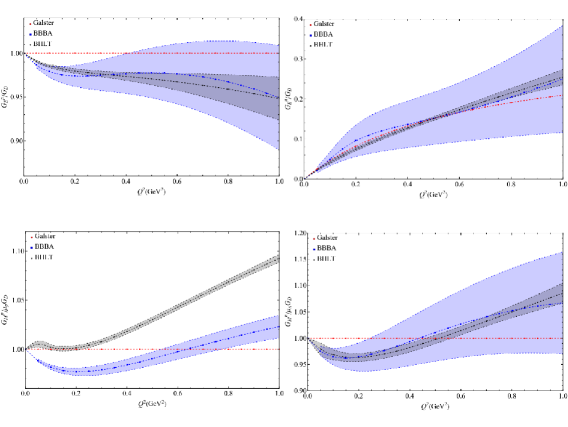
Figure 15: Comparison between the different electromagnetic form factor parametrizations shown for (Top) $G^{p}_{E}$ and $G^{n}_{E}$, and (Botton) $G^{p}_{M}$ and $G^{n}_{M}$. The red circle, blue square, and gray diamond data points represent the Galster, BBBA, and BHLT Parametrizations respectively.

C.1.2 BHLT Parametrization

The form factors in the BHLT parameterization [2] were determined from a global fit to electron scattering data and precise charge radius measurements. The form factors are expressed as a convergent expansion in $z(q^{2})$,

$$G_{E}^{p,n} = \sum_{k=0}^{k_{max}}a_{k}z(q^{2})^{k},$$

$$G_{M}^{p,n} = G_{M}^{p,n}(0)\sum_{k=0}^{k_{max}}b_{k}z(q^{2})^{k},$$

$$z(q^{2}) = \frac{\sqrt{t_{cut}-q^{2}}-\sqrt{t_{cut}-t_{0}}}{\sqrt{t_{cut}-q^{2}}+\sqrt{t_{cut}-t_{0}}},$$ (48)

where, $t_{cut}=4m_{\pi}^{2}$ and $t_{0}=-0.21\,$GeV². The form factor coefficients for the proton and neutron $a_{1}$ to $a_{4}$, and the corresponding covariant matrix for the uncertainty are provided in the supplementary material of [2].
To calculate the five unknown coefficients, namely $a_{0}$ and $a_{5}-a_{8}$, the normalization $G(0)$ ($G^{p}_{E}(0)=1$, $G^{n}_{E}(0)=0$ , $G^{p}_{M}(0)=\mu_{p}$, and $G^{n}_{M}(0)=\mu_{n}$) and the four sum rules in equation (6) from [2] are used:

$$G(0)-\sum_{k=0}^{8}a_{k}z(0)^{k}=0,\quad\sum_{k=0}^{8}a_{k}=0,\quad\sum_{k=1}^{8}ka_{k}=0$$

$$\sum_{k=2}^{8}k(k-1)a_{k}=0,\quad\sum_{k=3}^{8}k(k-1)(k-2)a_{k}=0\,.$$ (49)

In figure 15 we present a comparison of BBBA and BHLT parameterizations, as well as the historical Galster [46] parameterization that is sometimes used, e.g., in [4].

C.2 Axial form factor

With the exception of the historical dipole model, given in section 4.2, axial form factor parameterizations are extracted using $z$-expansion, where the axial form factor $F_{A}$ is given by:

$$F_{A}(q^{2})=\sum_{k=0}^{k_{max}}a_{k}z(q^{2})^{k},\quad\mbox{where}\quad z(q^{2})=\frac{\sqrt{t_{cut}-q^{2}}-\sqrt{t_{cut}-t_{0}}}{\sqrt{t_{cut}-q^{2}}+\sqrt{t_{cut}-t_{0}}}.$$ (50)

C.2.1 MBGH Parametrization

The axial nucleon form factor in the MBGH parametrization [34] was determined from charged-current neutrino-deuterium scattering data. The $z$-expansion from equation (50) is used to calculate the form factor for $k_{max}=8$ with, $t_{cut}=9m_{\pi}^{2}$ ($m_{\pi}=140$ MeV), and $t_{0}=-0.28\,$GeV². The coefficients for $k=1$ to $4$ and the covariant matrix are listed in [34]. The five remaining coefficients are determined from normalization, $F_{A}(0)=g_{A}=-1.2723$, and the sum rule constraints as in equation (C.1.2).

C.2.2 NME 22

The axial form factor by the Nuclear Matrix Element (NME) collaboration [37] is extracted from the results for the axial current between ground-state nucleons. The parametrization in the $\{4^{N\pi},2^{sim},\hat{z}^{2}\}$ fit is obtained using the $z$-expansion from equation (50) for $k_{max}=2$ with $t_{cut}=9m_{\pi}^{2}$ ($m_{\pi}=135$ MeV), and $t_{0}=-0.5\,$GeV². The three parameters and the covariant matrix can be found in [37].

C.2.3 Mainz 22

The $z$-expansion coefficients were extracted directly from lattice correlators by the Mainz group. Using the $z$-expansion from equation (50) for $k_{max}=2$ with, $t_{cut}=9m_{\pi}^{2}$ ($m_{\pi}=135$ MeV), and $t_{0}=0\,$GeV² the axial form factor was obtained. The coefficients for $k=0$ to $2$ and the covariant matrix for the three coefficients are listed in [38].

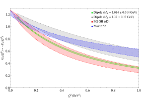
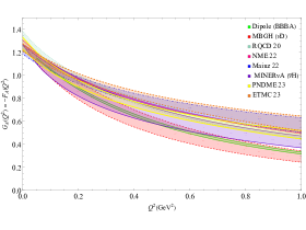
Figure 16: Comparison between the different axial form factor parameterizations implemented for neutrino scattering. Left: comparison between the models Mainz 22 and MBGH which span across the two dipole models with $M_{A}=1.35\pm 0.17$ GeV [15] and $M_{A}=1.014\pm 0.014$ GeV [44], respectively. Right: the comparison between Dipole (BBBA) using $M_{A}=1.014\pm 0.014$ GeV, MBGH [34], RQCD 20 [36], NME 22 [37], Mainz 22 [38], MINERvA [35], PNDME 23 [39] and ETMC 23 [40].

C.2.4 MINERvA

Axial form factor is extracted from the $\bar{\nu}$-hydrogen scattering using the plastic scintillator target of the MINERvA experiment [35]. The $z$-expansion from equation (50) is used to extract $F_{A}$ from the hydrogen cross-section for $k_{max}=8$, with $t_{cut}=9m_{\pi}^{2}$ ($m_{\pi}=140$ MeV), and $t_{0}=-0.75\,$GeV². The coefficients for $k=0$ to $4$ and the covariant matrix are listed in [35]. The five remaining coefficients are determined from normalization ($F_{A}(0)=g_{A}=-1.2723$) and the sum rule constraints in equation (C.1.2).

C.2.5 PNDME 23

The coefficients in $F_{A}$ are extracted using thirteen 2+1+1 flavor highly improved staggered quark (HISQ) ensembles. Using $k_{max}=2$ in equation (50), with $t_{cut}=9m_{\pi}^{2}$ ($m_{\pi}=135$ MeV), and $t_{0}=-0.25\,$GeV² the axial form factor is obtained. The coefficients for $k=0$ to $2$ and the covariant matrix are provided in [39].

C.2.6 ETMC 23

The axial form factor in Extended Twisted Mass Collaboration [40] is evaluated using three $N_{f}=2+1+1$ twisted mass fermion ensembles. The $z$-expansion from equation (50) is used to extract $F_{A}$ from the hydrogen cross-section, with $t_{cut}=9m_{\pi}^{2}$ ($m_{\pi}=135$ MeV), and $t_{0}=0\,$GeV². The coefficients for $k=0$ to $3$ and the covariant matrix are provided in [40].

C.2.7 RQCD 20

The two- and three-point correlation functions are extracted using EFT methods in [36]. They obtain fits and in turn extract ground state form factors. The $z$-expansion formalism is used to extract $F_{A}$, with $t_{cut}=9m_{\pi}^{2}$ and $t_{0}=-t_{cut}$. No error bars are given for the $z$-expansion coefficients in [36], only for the form factor itself. Thus, we plot the form factor in figure 16, but we do not use it in figures 13 and 14.

Appendix D Appendix: More plots for electron scattering

In figure 17 we present comparison of the RFG and CFG models to electron-carbon scattering data for more kinematical points. The points shown were also considered in [8].

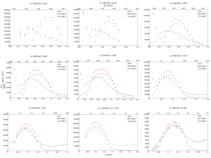
Figure 17: A comparison of double differential cross-section using RFG (red squares) and CFG (blue diamond) nuclear model with the carbon data for various incoming electron energy and scattering angles.

References

- [1] R. Bradford, A. Bodek, Howard Scott Budd, and J. Arrington. A New parameterization of the nucleon elastic form-factors. Nucl. Phys. B Proc. Suppl., 159:127–132, 2006, hep-ex/0602017.
- [2] Kaushik Borah, Richard J. Hill, Gabriel Lee, and Oleksandr Tomalak. Parametrization and applications of the low- nucleon vector form factors. Phys. Rev. D, 102(7):074012, 2020, 2003.13640.
- [3] Joanna Ewa Sobczyk. Intercomparison of lepton-nucleus scattering models in the quasielastic region. Phys. Rev. C, 96(4):045501, 2017, 1706.06739.
- [4] Joanna Ewa Sobczyk. Nuclear effects in neutrino-nucleus interactions: the role of spectral functions. PhD thesis, U. Valencia (main), 2019.
- [5] O. Benhar, A. Fabrocini, S. Fantoni, and I. Sick. Spectral function of finite nuclei and scattering of GeV electrons. Nucl. Phys. A, 579:493–517, 1994.
- [6] Omar Benhar, Pietro Coletti, and Davide Meloni. Electroweak nuclear response in quasi-elastic regime. Phys. Rev. Lett., 105:132301, 2010, 1006.4783.
- [7] M. Petraki, E. Mavrommatis, O. Benhar, John Walter Clark, A. Fabrocini, and S. Fantoni. Final state interactions in the response of nuclear matter. Phys. Rev. C, 67:014605, 2003, nucl-th/0201019.
- [8] Artur M. Ankowski, Omar Benhar, and Makoto Sakuda. Improving the accuracy of neutrino energy reconstruction in charged-current quasielastic scattering off nuclear targets. Phys. Rev. D, 91(3):033005, 2015, 1404.5687.
- [9] A. Gil, J. Nieves, and E. Oset. Many body approach to the inclusive (e, e-prime) reaction from the quasielastic to the Delta excitation region. Nucl. Phys. A, 627:543–598, 1997, nucl-th/9711009.
- [10] J. Nieves, Jose Enrique Amaro, and M. Valverde. Inclusive quasi-elastic neutrino reactions. Phys. Rev. C, 70:055503, 2004, nucl-th/0408005. [Erratum: Phys.Rev.C 72, 019902 (2005)].
- [11] Juan Nieves and Joanna Ewa Sobczyk. In medium dispersion relation effects in nuclear inclusive reactions at intermediate and low energies. Annals Phys., 383:455–496, 2017, 1701.03628.
- [12] P. Fernandez de Cordoba and E. Oset. Semiphenomenological approach to nucleon properties in nuclear matter. Phys. Rev. C, 46:1697–1709, 1992.
- [13] O. Buss, T. Gaitanos, K. Gallmeister, H. van Hees, M. Kaskulov, O. Lalakulich, A. B. Larionov, T. Leitner, J. Weil, and U. Mosel. Transport-theoretical Description of Nuclear Reactions. Phys. Rept., 512:1–124, 2012, 1106.1344.
- [14] K. Gallmeister, U. Mosel, and J. Weil. Neutrino-Induced Reactions on Nuclei. Phys. Rev. C, 94(3):035502, 2016, 1605.09391.
- [15] A. A. Aguilar-Arevalo et al. First Measurement of the Muon Neutrino Charged Current Quasielastic Double Differential Cross Section. Phys. Rev. D, 81:092005, 2010, 1002.2680.
- [16] Bhubanjyoti Bhattacharya, Richard J. Hill, and Gil Paz. Model independent determination of the axial mass parameter in quasielastic neutrino-nucleon scattering. Phys. Rev. D, 84:073006, 2011, 1108.0423.
- [17] Bhubanjyoti Bhattacharya, Gil Paz, and Anthony J. Tropiano. Model-independent determination of the axial mass parameter in quasielastic antineutrino-nucleon scattering. Phys. Rev. D, 92(11):113011, 2015, 1510.05652.
- [18] E. J. Moniz, I. Sick, R. R. Whitney, J. R. Ficenec, Robert D. Kephart, and W. P. Trower. Nuclear Fermi momenta from quasielastic electron scattering. Phys. Rev. Lett., 26:445–448, 1971.
- [19] K. S. Egiyan et al. Observation of nuclear scaling in the A(e, e-prime) reaction at x(B) greater than 1. Phys. Rev. C, 68:014313, 2003, nucl-ex/0301008.
- [20] K. S. Egiyan et al. Measurement of 2- and 3-nucleon short range correlation probabilities in nuclei. Phys. Rev. Lett., 96:082501, 2006, nucl-ex/0508026.
- [21] N. Fomin et al. New measurements of high-momentum nucleons and short-range structures in nuclei. Phys. Rev. Lett., 108:092502, 2012, 1107.3583.
- [22] A. Tang et al. n-p short range correlations from (p, 2p + n) measurements. AIP Conf. Proc., 549(1):451–454, 2000, nucl-ex/0009009.
- [23] E. Piasetzky, M. Sargsian, L. Frankfurt, M. Strikman, and J. W. Watson. Evidence for the strong dominance of proton-neutron correlations in nuclei. Phys. Rev. Lett., 97:162504, 2006, nucl-th/0604012.
- [24] R. Shneor et al. Investigation of proton-proton short-range correlations via the C-12(e, e-prime pp) reaction. Phys. Rev. Lett., 99:072501, 2007, nucl-ex/0703023.
- [25] R. Subedi et al. Probing Cold Dense Nuclear Matter. Science, 320:1476–1478, 2008, 0908.1514.
- [26] I. Korover et al. Probing the Repulsive Core of the Nucleon-Nucleon Interaction via the Triple-Coincidence Reaction. Phys. Rev. Lett., 113(2):022501, 2014, 1401.6138.
- [27] Or Hen, Bao-An Li, Wen-Jun Guo, L. B. Weinstein, and Eli Piasetzky. Symmetry Energy of Nucleonic Matter With Tensor Correlations. Phys. Rev. C, 91(2):025803, 2015, 1408.0772.
- [28] Bao-Jun Cai and Bao-An Li. Nuclear Equation of State and Single-nucleon Potential from Gogny-like Energy Density Functionals Encapsulating Effects of Nucleon-nucleon Short-range Correlations. 10 2022, 2210.10924.
- [29] Carolyn Raithel, Vasileios Paschalidis, and Feryal Özel. Realistic finite-temperature effects in neutron star merger simulations. Phys. Rev. D, 104(6):063016, 2021, 2104.07226.
- [30] Carolyn A. Raithel, Feryal Ozel, and Dimitrios Psaltis. Finite-temperature extension for cold neutron star equations of state. Astrophys. J., 875(1):12, 2019, 1902.10735.
- [31] O. Hen, A. W. Steiner, E. Piasetzky, and L. B. Weinstein. Analysis of Neutron Stars Observations Using a Correlated Fermi Gas Model, 8 2016, 1608.00487.
- [32] B. Schmookler et al. Modified structure of protons and neutrons in correlated pairs. Nature, 566(7744):354–358, 2019, 2004.12065.
- [33] Luis Alvarez-Ruso et al. Recent highlights from GENIE v3. Eur. Phys. J. ST, 230(24):4449–4467, 2021, 2106.09381.
- [34] Aaron S. Meyer, Minerba Betancourt, Richard Gran, and Richard J. Hill. Deuterium target data for precision neutrino-nucleus cross sections. Phys. Rev. D, 93(11):113015, 2016, 1603.03048.
- [35] T. Cai et al. Measurement of the axial vector form factor from antineutrino–proton scattering. Nature, 614(7946):48–53, 2023.
- [36] Gunnar S. Bali, Lorenzo Barca, Sara Collins, Michael Gruber, Marius Löffler, Andreas Schäfer, Wolfgang Söldner, Philipp Wein, Simon Weishäupl, and Thomas Wurm. Nucleon axial structure from lattice QCD. JHEP, 05:126, 2020, 1911.13150.
- [37] Sungwoo Park, Rajan Gupta, Boram Yoon, Santanu Mondal, Tanmoy Bhattacharya, Yong-Chull Jang, Bálint Joó, and Frank Winter. Precision nucleon charges and form factors using (2+1)-flavor lattice QCD. Phys. Rev. D, 105(5):054505, 2022, 2103.05599.
- [38] Dalibor Djukanovic, Georg von Hippel, Jonna Koponen, Harvey B. Meyer, Konstantin Ottnad, Tobias Schulz, and Hartmut Wittig. Isovector axial form factor of the nucleon from lattice QCD. Phys. Rev. D, 106(7):074503, 2022, 2207.03440.
- [39] Yong-Chull Jang, Rajan Gupta, Tanmoy Bhattacharya, Boram Yoon, and Huey-Wen Lin. Nucleon isovector axial form factors. Phys. Rev. D, 109(1):014503, 2024, 2305.11330.
- [40] Constantia Alexandrou, Simone Bacchio, Martha Constantinou, Jacob Finkenrath, Roberto Frezzotti, Bartosz Kostrzewa, Giannis Koutsou, Gregoris Spanoudes, and Carsten Urbach. Nucleon axial and pseudoscalar form factors using twisted-mass fermion ensembles at the physical point. Phys. Rev. D, 109(3):034503, 2024, 2309.05774.
- [41] Omar Benhar, Donal Day, and Ingo Sick. An Archive for quasi-elastic electron-nucleus scattering data. 3 2006, nucl-ex/0603032.
- [42] Quasielastic Electron Nucleus Scattering Archive. http://discovery.phys.virginia.edu/research/groups/qes-archive.
- [43] R. L. Workman et al. Review of Particle Physics. PTEP, 2022:083C01, 2022.
- [44] A. Bodek, S. Avvakumov, R. Bradford, and Howard Scott Budd. Vector and Axial Nucleon Form Factors:A Duality Constrained Parameterization. Eur. Phys. J. C, 53:349–354, 2008, 0708.1946.
- [45] Oleksandr Tomalak, Rajan Gupta, and Tanmoy Bhattacharya. Confronting the axial-vector form factor from lattice QCD with MINERvA antineutrino-proton data. Phys. Rev. D, 108(7):074514, 2023, 2307.14920.
- [46] S. Galster, H. Klein, J. Moritz, K. H. Schmidt, D. Wegener, and J. Bleckwenn. Elastic electron-deuteron scattering and the electric neutron form factor at four-momentum transfers 5fmfm-2. Nucl. Phys. B, 32:221–237, 1971.