Solar neutrinos and leptonic spin forces

Abstract

We quantify the effects on the evolution of solar neutrinos of light spin-zero particles with pseudoscalar couplings to leptons and scalar couplings to nucleons. In this scenario the matter potential sourced by the nucleons in the Sun’s matter gives rise to spin precession of the relativistic neutrino ensemble. As such the effects in the solar observables are different if neutrinos are Dirac or Majorana particles. For Dirac neutrinos the spin-flavour precession results into left-handed neutrino to right-handed neutrino (i.e., active–sterile) oscillations, while for Majorana neutrinos it results into left-handed neutrino to right-handed antineutrino (i.e., active-active) oscillations. In both cases this leads to distortions in the solar neutrino spectrum which we use to derive constraints on the allowed values of the mediator mass and couplings via a global analysis of the solar neutrino data. In addition for Majorana neutrinos spin-flavour precession results into a potentially observable flux of solar electron antineutrinos at the Earth which we quantify and constrain with the existing bounds from Borexino and KamLAND.

1 Introduction

The Standard Model (SM) has been extensively tested at a plethora of experimental environments and so far no definitive deviation from its predictions has been observed at the highest energy scales probed, neither for what concerns the interactions of known particles Pasztor:2019rqu nor through the appearance of new heavy states Yuan:2020fyf . Yet physics beyond the Standard Model (BSM) is required to address the well-known shortcomings of the SM. The obvious conclusion seems to be that there must be a mass gap between the electroweak and the BSM scales. There remains, however, the interesting possibility of new light states that have escaped detection so far because they are coupled feebly with the SM (see Ref. Antel:2023hkf for recent review) but can produce tiny yet observable effects — in particular when coherently enhanced. The paradigmatic example is light spin-zero axion-like particles: they entered the spectrum of BSM physics motivated by the strong CP problem Weinberg:1977ma ; Wilczek:1977pj ; Peccei:1977hh and they soon became also a viable solution to the dark matter puzzle Preskill:1982cy ; Abbott:1982af ; Dine:1982ah . Another notable example is the Majoron, associated with the spontaneous breaking of the lepton number Chikashige:1980ui ; Gelmini:1980re in models of neutrino mass generation.

In most generality a spin-zero field $\phi$ can couple to the SM model fermions $\psi$ with a scalar (i.e., spin-independent) coupling $(\bar{\psi}\psi\phi)$, or with a pseudoscalar spin-dependent coupling $(\bar{\psi}\gamma^{5}\psi\phi)$. In this case they generate monopole-monopole forces, as well as monopole-dipole and dipole-dipole forces Moody:1984ba between non-relativistic SM fermions. In particular the dipole interaction is known to appear as an effective background magnetic field proportional to the gradient of the $\phi$ field which generates the precession of the fermion spin.

Recently, monopole-dipole forces have been invoked in the context of the measurement of the muon $g-2$ which has put in question the consistency with the Standard Model (SM) theoretical predictions Aoyama:2020ynm ; Borsanyi:2020mff . Concretely, the experimental result in Ref. Muong-2:2023cdq for the muon anomalous magnetic moment is larger than the data-driven value predicted in the SM Aoyama:2020ynm by about $3$–$4\sigma$. In this context Refs. Janish:2020knz ; Agrawal:2022wjm ; Davoudiasl:2022gdg proposed such monopole-dipole interaction with the scalar coupling $g_{s}^{N}$ to nucleons acting as a source of the field $\phi$, whose pseudoscalar coupling to the muon, $g_{p}^{\mu}$, will alter its precession frequency and could be interpreted as a contribution to $g-2$. For sufficently light $\phi$ field, $m_{\phi}\sim 10^{-14}$ eV, the long range of the force leads to a coherent enhancement with all atoms in the Earth contributing to the gradient of the scalar field at Earth’s surface where muon spin experiments are performed. The required value to explain the $(g-2)_{\mu}$ anomaly is $g_{s}^{N}g_{p}^{\mu}\gtrsim 10^{-30}$ Agrawal:2022wjm ; Davoudiasl:2022gdg .

New interactions of leptons are known to have also interesting effects in the neutrino sector because they can affect their flavour evolution when traveling through large regions of matter, as is the case for solar neutrinos. In the SM this leads to the well-known Mikheev-Smirnov-Wolfenstein (MSW) mechanism Wolfenstein:1977ue ; Mikheev:1986gs with a well determined potential difference between the electron neutrino and the other flavours. New flavour-dependent interactions can modify the matter potential and consequently alter the pattern of flavour transitions, thus leaving imprints in the oscillation data. In the Standard Model the generated potential is proportional to the electron density at the neutrino position because forward elastic scattering takes place in the limit of zero momentum transfer, so as long as the range of the interaction is shorter than the scale over which the matter density extends, the effective matter potential can be obtained in the contact interaction approximation between the neutrinos and the matter particles. Conversely, if the mediator is extremely light the contact interaction approximation is no longer valid, and the flavour dependent forces between neutrino and matter particles become long-range. Neutrino propagation can still be described in terms of a matter potential, which however is no longer simply determined by the number density of particles in the medium at the neutrino position, but it depends instead on the average of the matter density within a radius $\sim 1/M_{\text{med}}$ around it Grifols:2003gy ; Joshipura:2003jh ; GonzalezGarcia:2006vp ; Davoudiasl:2011sz ; Wise:2018rnb ; Coloma:2020gfv .

Moreover if the force couples to the lepton spin, irrespective of its flavour dependence, it can flip the helicity of the neutrino, a process usually refered to as spin-flavour precession (SFP) which takes place, for example, by interaction with the solar magnetic field in the presence of a flavour-dependent neutrino magnetic-moment Cisneros:1970nq ; Okun:1986hi ; Okun:1986na ; Okun:1986uf ; Voloshin:1986ty , and that can be resonantly enhanced by solar matter Akhmedov:1987nc ; Lim:1987tk as well. An interesting characteristic of such spin forces acting on the neutrino is that their observable effects are different if neutrinos are Dirac or Majorana fermions. For Dirac neutrinos SFP converts a fraction of the left-handed neutrinos into right-handed neutrinos which escape detection. In the context of neutrino oscillations this corresponds to an active-sterile neutrino oscillation which would leave an imprint in the solar neutrino data. If, on the contrary, neutrinos are Majorana, then SFP results in the convertion into right-handed antineutrinos which, besides its effect on solar neutrino data, can lead to a small but potentially observable flux of solar electron antineutrinos at the Earth.

At present, the global analysis of data from oscillation experiments provides some of the strongest constraints on the size of interactions affecting the neutrino flavour evolution either in the contact GonzalezGarcia:2011my ; Gonzalez-Garcia:2013usa ; Esteban:2018ppq ; Coloma:2023ixt ; Coloma:2022umy or the long-range Grifols:2003gy ; Joshipura:2003jh ; GonzalezGarcia:2006vp ; Coloma:2020gfv regime, while the experimental bounds on the solar antineutrino flux provides strong bounds on the neutrino magnetic-moment due to its associated SFP effect (for a recent analysis see Ref. Akhmedov:2022txm and references therein).

With this motivation in this article we study the effect on the neutrinos flavour oscillations of a pseudoscalar coupling between neutrinos and a spin-zero particle with scalar couplings to the nucleons. In Sec. 2 we present the formalism to study neutrino propagation in the presence of these interactions and the generated helicity-flipping potential (with details on its derivation in appendix A). In Sec. 3 we derive bounds on such interaction (as a function of the mediator mass) from the global analysis of present solar and KamLAND data for either Dirac or Majorana neutrinos, and from the solar antineutrino flux bounds for the case of Majorana neutrinos. Finally, in Sec. 4 we discuss these bounds in the context of the current limits from charged muon results, and present our conclusions.

2 Formalism

We consider the interactions of a field $\phi$ with scalar couplings to the nucleons and pseudoscalar couplings to neutrinos:

$$\mathcal{L}_{\phi}=\sum_{f=n,p}g_{s}^{f}\phi\bar{f}f+i\,[g_{p}^{\nu}]^{\alpha\beta}\phi\,\overline{\nu}_{\alpha}\gamma^{5}\nu_{\beta}\,,$$ (1)

where $g_{p}^{\nu}$ parametrize the pseudoscalar couplings to the spin of the neutrinos, which in its most generality is a $3\times 3$ hermitian matrix in the neutrino flavour space.

Considering solar neutrinos, the interactions in Eq. (1) will generate a flavour dependent potential sourced by the nucleons in the Sun which will affect the flavour evolution of the neutrinos and can lead to observable signatures. We present in Appendix A the derivation of this potential. In brief, we find that the interactions in Eq. (1) generate a spin-flip potential on a neutrino of energy $E_{\nu}$ at position $\vec{x}$ of the form

$$V_{\text{sp}}(\vec{x})=-\frac{g_{s}^{f}g_{p}^{\nu}}{4E_{\nu}}\mathcal{E}_{\perp}(\vec{x})$$ (2)

where $\mathcal{E}_{\perp}$ is the size of the transverse component (with respect to the neutrino trajectory) of a vector field $\vec{\mathcal{E}}$ defined as

$$\vec{\mathcal{E}}(\vec{x})\equiv\frac{1}{2\pi}\vec{\nabla}_{x}\int N_{f}(\vec{\rho})\,\frac{e^{-m_{\phi}|\vec{\rho}-\vec{x}|}}{|\vec{\rho}-\vec{x}|}\,d^{3}\vec{\rho}\,\equiv\frac{2}{m_{\phi}^{2}}\vec{\nabla}\hat{N}_{f}(\vec{x},m_{\phi})\,.$$ (3)

In writing Eq. (3) we have introduced the quantity $\hat{N}_{f}(\vec{x},m_{\phi})$ which represents the potential-weighted matter density within a radius $\sim 1/m_{\phi}$ around the neutrino location Grifols:2003gy ; Joshipura:2003jh ; GonzalezGarcia:2006vp ; Davoudiasl:2011sz ; Wise:2018rnb . Its normalization factor ensures that $\hat{N}_{f}(\vec{x},m_{\phi})\to N_{f}(\vec{x})$ for $m_{\phi}\to\infty$, because that is the limit in which one should recover the contact interaction expectation (i.e., the neutrino wave packet localized at position $\vec{x}$ should be directly sensitive to the number density distribution $N_{f}(\vec{x})$ of fermion $f$ at such point).

Denoting by $r\equiv|\vec{x}-\vec{x}_{\odot}|$ the distance from the center of the Sun $\vec{x}_{\odot}$ and taking into account the spherical symmetry of the solar matter distribution $N_{f}^{\odot}(r)$, we see that $\hat{N}_{f}(\vec{x},m_{\phi})$ simplifies to $\hat{N}_{f}(r,m_{\phi})$ with:

$$\hat{N}_{f}(r,m_{\phi})=\frac{m_{\phi}}{2\,r}\int_{0}^{R_{\odot}}\rho\,N_{f}^{\odot}(\rho)\big{[}e^{-m_{\phi}|\rho-r|}-e^{-m_{\phi}(\rho+r)}\big{]}\,d\rho\,.$$ (4)

Notice that since $\hat{N}_{f}(r,m_{\phi})$ only depends on the radial distance to the center of the Sun, the direction of the vector $\vec{\mathcal{E}}(\vec{x})$ is radial. As the spin-flip potential is proportional to the component of $\vec{\mathcal{E}}$ orthogonal to the neutrino direction, it is clear that it will vanish for trajectories along the line connecting the solar center and the center of the Earth. For neutrinos at a transverse distance $b$ from the line connecting the Earth and Sun centers, and at a radial distance $r$ from the center of the Sun, the potential is

$$V_{\text{sp}}(r,b)=-\frac{g_{s}^{N}g_{p}^{\nu}}{2E_{\nu}\,m_{\phi}^{2}}\cdot\frac{b}{r}\cdot\frac{d\hat{N}_{f}(r,m_{\phi})}{dr}\,.$$ (5)

In Fig. 1 we plot the value of this potential (for different values of $m_{\phi}$) at a given position $(b,z)$, where $b$ is the transverse distance to the line connecting the Sun and Earth centers, and $z=\sqrt{r^{2}-b^{2}}$ is the distance along the Sun-Earth direction (which, as we will see below, is the variable parametrizing the neutrino trajectory). For the sake of concretness we show the results for $g_{s}^{p}=g_{s}^{n}\equiv g_{s}^{N}$.

From the figure we see that, as expected, the potential decreases as $b\to 0$. However, it increases very rapidly with $b$ and it reaches its maximum for values of $b$ well within the neutrino production region $b\lesssim 0.3\,R_{\odot}$. Quantiatively we see that for the $m_{\phi}$ considered here the characteristic values of the potential inside the solar core are comparable with the inverse of the oscillation length of solar neutrinos with energy $E_{\nu}$, $E_{\nu}/\lambda\sim\Delta m^{2}_{21}\sim 10^{-4}~{}\text{eV}^{2}$ for $g_{s}^{N}g_{p}^{\nu}\sim 10^{-30}$ within the range of values of the coupling to muons proposed to account for the $(g-2)_{\mu}$ anomaly Agrawal:2022wjm ; Davoudiasl:2022gdg .

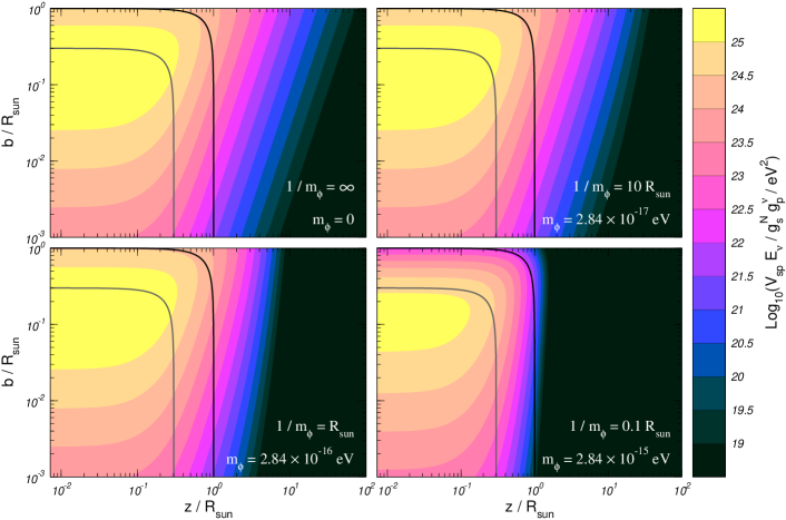
Figure 1: Isocontours of the potential $V_{sp}$ sourced by nucleons with coupling $g_{s}^{N}$ to $\phi$ felt by $\nu$ with coupling $g_{p}^{\nu}$ to $\phi$ as a function of $b$ (its transverse distance to the line connecting the Sun and Earth centers) and $z$ (the distance along the Sun-Earth direction characterizing its trajectory to the Earth) for several values of $m_{\phi}$. For reference the black lines represent the position of the edge of the Sun, $\sqrt{b^{2}+z^{2}}=R_{\odot}$, and the outer edge of the solar core, $\sqrt{b^{2}+z^{2}}=0.3\,R_{\odot}$.

To account for the effect of this potential in the solar neutrino observables we need to solve the evolution equation for the neutrino ensemble. Since the potential flips the helicity of the neutrino, such equation is different for Dirac and Majorana neutrinos. For a Dirac neutrino the evolution equation for its flavour components $\vec{\nu}\equiv(\nu_{e},\nu_{\mu},\nu_{\tau})^{T}$ reads

$$i\,\frac{d}{dt}\begin{pmatrix}\vec{\nu}_{L}(t)\\ \vec{\nu}_{R}(t)\end{pmatrix}=\begin{pmatrix}H^{\nu}(r)&V_{\text{sp}}(r,b)\\ V_{\text{sp}}(r,b)^{\dagger}&H_{\text{vac}}\end{pmatrix}\begin{pmatrix}\vec{\nu}_{L}(t)\\ \vec{\nu}_{R}(t)\end{pmatrix},$$ (6)

where, given the large distance between the Sun and the Earth, we can assume with high precision that the neutrino travels along a trajectory which runs parallel to the line connecting the Sun and Earth centers, so that its distance $b$ from such line remains constant during propagation. Denoting by $z$ the longitudinal position of the neutrino along its trajectory, we have that at a given time $t$ the distance from the neutrino location to the center of the Sun is given by $r=\sqrt{b^{2}+(z-z_{0})^{2}}$ with $z=z_{0}+ct$.

For a Majorana neutrino the evolution equation is

$$i\,\frac{d}{dt}\begin{pmatrix}\vec{\nu}_{L}(t)\\ \vec{\overline{\nu}}_{R}(t)\end{pmatrix}=\begin{pmatrix}H^{\nu}(r)&V_{\text{sp}}(r,b)\\ V_{\text{sp}}(r,b)^{\dagger}&H^{\overline{\nu}}(r)\end{pmatrix}\begin{pmatrix}\vec{\nu}_{L}(t)\\ \vec{\overline{\nu}}_{R}(t)\end{pmatrix},$$ (7)

where

$$H^{\nu}(r)=H_{\text{vac}}+H_{\text{mat}}(r)\quad\text{and}\quad H^{\overline{\nu}}(r)=[H_{\text{vac}}-H_{\text{mat}}(r)]^{*}\,.$$ (8)

Here $H_{\text{vac}}$ is the vacuum part which in the flavour basis $(\nu_{e},\nu_{\mu},\nu_{\tau})$ reads

$$H_{\text{vac}}=U_{\text{vac}}D_{\text{vac}}U_{\text{vac}}^{\dagger}\quad\text{with}\quad D_{\text{vac}}=\frac{1}{2E_{\nu}}\mathop{\mathrm{diag}}(0,\Delta m^{2}_{21},\Delta m^{2}_{31})$$ (9)

where $U_{\text{vac}}$ denotes the three-lepton mixing matrix in vacuum Pontecorvo:1967fh ; Maki:1962mu ; Kobayashi:1973fv . Following the convention of Ref. Coloma:2016gei , we define $U_{\text{vac}}=R_{23}(\theta_{23})R_{13}(\theta_{13})\tilde{R}_{12}(\theta_{12},\delta_{\text{CP}})$, where $R_{ij}(\theta_{ij})$ is a rotation of angle $\theta_{ij}$ in the $ij$ plane and $\tilde{R}_{12}(\theta_{12},\delta_{\text{CP}})$ is a complex rotation by angle $\theta_{12}$ and phase $\delta_{\text{CP}}$. $H_{\text{mat}}(r)$ is the matter potential due to the SM weak interactions, which in the flavour basis takes the diagonal form

$$H_{\text{mat}}(r)=\frac{G_{F}}{\sqrt{2}}\mathop{\mathrm{diag}}\Big{[}2N_{e}(r)-N_{n}(r),\,-N_{n}(r),\,-N_{n}(r)\Big{]}$$ (10)

and $N_{e}(r)$ and $N_{n}(r)$ are the electron and neutron number density at distance $r$ from the solar center.

We numerically solve the evolution equation from the production point of the ${\nu_{e}}_{L}$ in the Sun to the Earth. With our choice of variables we can characterize the production point by its radial distance $r_{0}$ from the center of the Sun, its transverse distance $b$ from the line connecting the Sun-Earth centers, and the angle $\phi$ in that transverse plane, and we are left with two discrete possibilities $\vec{x}_{0}^{\pm}=(\pm\sqrt{r_{0}^{2}-b^{2}},b\cos\phi_{0},b\sin\phi_{0})$ where positive (negative) sign corresponds to neutrinos produced in the hemisphere of the Sun which is closer (further) from the Earth. In this way we obtain the oscillation probability into $\nu_{\alpha}$ (here denoting generically either a left-handed neutrino state, or a right-handed neutrino for Dirac and a right-handed antineutrino for Majorana), $P_{e\alpha}(\vec{x}_{0}^{\pm},E_{\nu})$. In the Standard Solar Models the probability distribution of the neutrino production point only depends on the radial distance to the center of the Sun, $r_{0}$ (with different distributions for the different neutrino production reactions) so it is convenient to define

$$P_{e\alpha}(r_{0},E_{\nu})\equiv\frac{1}{4\pi}\int d\Omega\,P_{e\alpha}(\vec{x}_{0},E_{\nu})=\frac{1}{4\pi r_{0}}\int_{0}^{r_{0}}db\,\frac{b}{\sqrt{r_{0}^{2}-b^{2}}}\int_{0}^{2\pi}d\phi\,\sum_{\pm}P_{e\alpha}(\vec{x}_{0}^{\pm},E_{\nu})\,.$$ (11)

As mentioned above each of the eight reactions producing solar neutrinos — labeled by $i=1\dots 8$ for pp, $\mbox{}^{7}\text{Be}$, pep, $\mbox{}^{13}\text{N}$, $\mbox{}^{15}\text{O}$, $\mbox{}^{17}\text{F}$, $\mbox{}^{8}\text{B}$, and hep — generates neutrinos with characteristic distributions $\mathcal{R}_{i}(r_{0})$ (normalized to one) which are energy independent. Thus we can obtain the mean survival probability for a neutrino of energy $E_{\nu}$ produced in reaction $i$ as

$$P^{i}_{e\alpha}(E_{\nu})=\int_{0}^{R_{\odot}}dr_{0}\,\mathcal{R}_{i}(r_{0})\,P_{e\alpha}(r_{0},E_{\nu})$$ (12)

and with those obtain the predictions for the solar observables in our analysis.

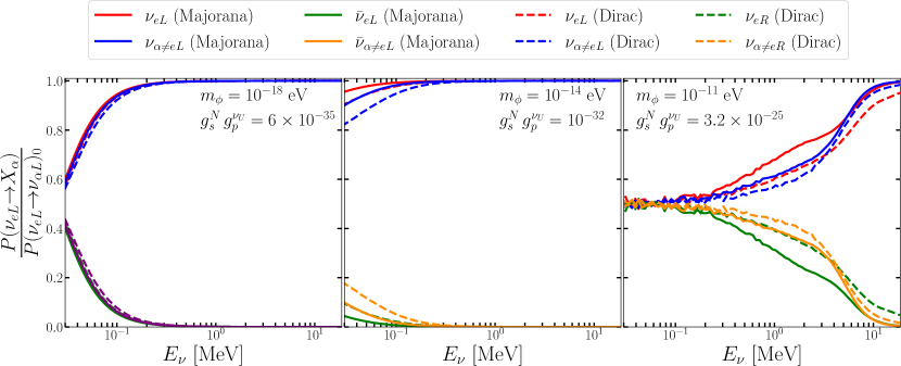
Figure 2: Relevant oscillation probabilities of solar $\nu_{eL}$ into left and right neutrinos (antineutrinos) of flavour $\alpha$ divided by $P(\nu_{e_{L}}\to\nu_{\alpha L})_{0}$ (the probability for zero coupling to the $\phi$ field) as a function of the neutrino energy for different values of model parameters as labeled in the figure. Oscillation parameters have been fixed to $\Delta m^{2}_{21}=7.4\times 10^{-5}~{}\text{eV}^{2}$, $\sin^{2}\theta_{12}=0.303$, $\sin^{2}\theta_{13}=0.02203$, $\Delta m^{2}_{31}=2.5\times 10^{-3}~{}\text{eV}^{2}$, $\sin^{2}\theta_{23}=0.5$, and $\delta_{\text{CP}}=0$.

In what follows, for the sake of concreteness, we are going to focus on four cases: three in which $\phi$ couples to a specific flavour $\gamma$ and a fourth in which the coupling is universal in flavour space

$$[g_{p}^{\nu}]^{\alpha\beta}=g_{p}^{\nu_{\gamma}}\,\delta^{\alpha\gamma}\delta^{\beta\gamma}\enspace\text{for}\enspace\gamma\in\{e,\mu,\tau\}\,,\quad\text{and}\quad[g_{p}^{\nu}]^{\alpha\beta}=g_{p}^{\nu_{U}}\,\delta^{\alpha\beta}\enspace\text{for universal}.$$ (13)

As illustration we plot in Fig. 2 the relevant oscillation probabilities for Dirac and Majorana cases as a function of the neutrino energy. The figure is shown for the case of coupling to $\nu_{U}$ but the behavior is qualitatively the same for couplings to $\nu_{e}$, $\nu_{\mu}$ or $\nu_{\tau}$. We assume fixed oscillation parameters $\Delta m^{2}_{21}=7.4\times 10^{-5}~{}\text{eV}^{2}$, $\sin^{2}\theta_{12}=0.303$, $\sin^{2}\theta_{13}=0.02203$, $\Delta m^{2}_{31}=2.5\times 10^{-3}~{}\text{eV}^{2}$, $\sin^{2}\theta_{23}=0.5$, and $\delta_{\text{CP}}=0$, and display different values for the two model parameters ($m_{\phi}$, $g_{s}^{N}g_{p}^{\nu_{U}}$). In the left (central) panel $m_{\phi}$ is within the infinite (contact) range interaction and the coupling constants are close to what will be the maximum allowed value, while the right panel corresponds to parameters which are well within the ruled out region. As seen in the figure the relevant probabilities are not very different for Dirac and Majorana neutrinos. Most importantly the figure shows that for moderate values of the model parameters the new interaction has largest effect on the disappearance of $\nu_{eL}$ and the appearance of $\nu_{\alpha\neq e,L}$ and $\nu_{\alpha R}$ ($\overline{\nu}_{\alpha R}$) for Dirac (Majorana) neutrinos with the lowest energies. This is expected as the potential in Eq. (2) is inversely proportional to the neutrino energy, as characteristic of interactions with spin-zero mediators GonzalezGarcia:2006vp . This is at a difference with the helicity-conserving MSW potential of Eq. (10) (or with any vector interaction in general Coloma:2020gfv ), and with the helicity-flip potential generated by a neutrino magnetic moment Akhmedov:1987nc ; Lim:1987tk which are independent of the neutrino energy. We also see that for these cases the relative effect on disappearance of $\nu_{eL}$ with $\sim\mathcal{O}(\text{10-100})$ KeV energy is larger than the $\overline{\nu}_{eR}$ appearance at MeV. These two facts are of relevance in the derivation of the bounds from the analysis of the solar neutrino and antineutrino data as we describe next.

3 Results

We first perform a global fit to solar neutrino oscillation data in the framework of three massive neutrinos including the new neutrino-matter interactions generated by the Lagrangian in Eq. (1) with the four choices of pseudoscalar couplings to neutrinos in Eq. (13). For the detailed description of the methodology we refer to our latest published global analysis NuFIT-5.0 Esteban:2020cvm to which we have included the data additions in NuFIT-5.3 nufit-5.3 . For solar neutrinos the analysis includes the total rates from the radiochemical experiments Chlorine Cleveland:1998nv , Gallex/GNO Kaether:2010ag , and SAGE Abdurashitov:2009tn , the spectral and zenith data from the four phases of Super-Kamiokande in Refs. Hosaka:2005um ; Cravens:2008aa ; Abe:2010hy including the latest SK4 2970-day energy and day/night spectrum Super-Kamiokande:2023jbt , the results of the three phases of SNO in the form of the day-night spectrum data of SNO-I Aharmim:2007nv and SNO-II Aharmim:2005gt and the three total rates of SNO-III Aharmim:2008kc , and the spectra from Borexino Phase-I Bellini:2011rx ; Bellini:2008mr , Phase-II Borexino:2017rsf , and Phase-III BOREXINO:2022abl . In the framework of three-neutrino mixing the oscillation probabilities for solar neutrinos dominantly depend on $\theta_{12}$ and $\Delta m^{2}_{21}$, for which relevant constraints arise from the analysis of the KamLAND reactor data, hence we include in our fit the separate DS1, DS2, DS3 spectra from KamLAND Gando:2013nba . Finally, let us mention that, in principle, the Earth matter nucleons also generate a spin-flavour precession potential which could affect the evolution of the KamLAND reactor antineutrinos as well as the day and night solar neutrino variations. Quantitatively, however, for the range of model parameters considered here this effect is negligible compared to that induced by the Sun, and it can therefore be safely neglected.

In what respect the relevant parameter space, Eqs. (6) and (7) are a set of six coupled linear differential equations whose solution depends on the two model parameters ($m_{\phi}$, $g_{s}^{N}g_{p}^{\nu_{a}}$) (for $a=e,\mu,\tau$ or $U$) and the six oscillation parameters, $\theta_{12}$, $\theta_{13}$, $\theta_{23}$, $\Delta m^{2}_{21}$, $\Delta m^{2}_{32}$, and $\delta_{\text{CP}}$. However, as it is well-know, the present determination of $\Delta m^{2}_{32}$ — derived dominantly from atmospheric, long-baseline accelerator, and medium-baseline reactor neutrino experiments — implies that the solar neutrino oscillations driven by $\Delta m^{2}_{32}/E_{\nu}$ are averaged out. Thus in our numerical evaluations we fix it to its present best-fit value, but any other value would yield the same result as long as we remain in the regime of averaged $\Delta m^{2}_{32}$ oscillations. In the standard $3\nu$ oscillation scenario $\nu_{\mu}$ and $\nu_{\tau}$ are totally indistinguishable at the energy scale of solar and reactor experiments, hence also the dependence on $\theta_{23}$ and $\delta_{\text{CP}}$ drops out in the evaluation of the solar observables. Including the flavour dependent scalar-pseudoscalar potential reintroduces a mild dependence on $\theta_{23}$ and $\delta_{\text{CP}}$ (except for the flavour-universal case $a=U$), but quantitatively the phenomenology of solar neutrino data is still dominated by $\Delta m^{2}_{21}$ and $\theta_{21}$. The dependence on $\theta_{13}$ is much weaker than its present precision from medium-baseline reactor experiments (in particular from Daya-Bay DayaBay:2022orm ), while the impact of the CP phase is very marginal. So we can safely fix $\theta_{13}$ to its current best-fit value from NuFIT-5.3 $\sin^{2}\theta_{13}=0.02203$ and set $\delta_{\text{CP}}=0$. In what respects $\theta_{23}$, for coupling to specific flavours $a=e,\mu,\tau$ we marginalize it within the allowed range from the global oscillation analysis by adding a prior for $\sin^{2}\theta_{23}$ from NuFIT-5.3 nufit-5.3 to the $\chi^{2}$ function of the solar and KamLAND experiments. Altogether the parameter space to be explored is five-dimensional.

We perform the analysis for both Dirac and Majorana neutrinos. Besides the different $\nu_{eL}$ oscillation probabilities resulting from the evolution equations Eqs. (6) and (7), there are also differences in the evaluation of the neutrino-electron elastic scattering event rates in Borexino, SNO and SK: while for the Dirac case the produced $\nu_{\alpha R}$ does not interact in the detector, for Majorana neutrinos the $\overline{\nu}_{\alpha R}$ do interact (albeit with a different cross section than the corresponding $\nu_{\alpha L}$ neutrinos) and such interactions must be included in the evaluation of the event rates. Furthermore the CC event rate at SNO can also be different for Dirac and Majorana because the $\overline{\nu}_{eR}$ interaction will produce a positron and two neutrons which may or may not be discriminated. Lacking the details for a proper estimation, we have performed the analysis under two extreme hypothesis: either assuming that the $e^{+}$ is recognized and the whole event is rejected, or that the positron is misidentified as an electron and it contributes as a CC event plus two additional NC events because of the generated neutrons. We have verified that the final bounds obtained under the two assumptions are the same.

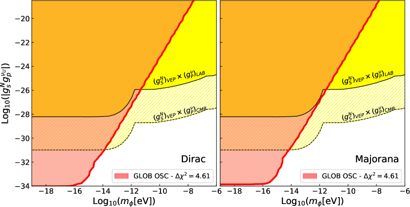
Figure 3: Excluded region at 90% CL in the ($m_{\phi}$, $g_{s}^{N}g_{p}^{\nu_{U}}$) plane by the global analysis of solar neutrino data after marginalization over the relevant oscillation parameters ($\Delta m^{2}_{21}$, $\theta_{12}$) while keeping the other oscillation parameters fixed as described in the text. Left (right) panel corresponds to Dirac (Majorana) neutrinos. For comparison we show as yellow region the bounds on the product of couplings (see Sec. 4).

Altogether we find that the inclusion of the new interaction does not lead to any significant improvement on the description of the data, and in fact the overall best-fit $\chi^{2}$ in the five-dimensional parameter space is the same as in the standard $3\nu$ oscillation scenario. Consequently the statistical analysis results into bounds on the allowed range of the scalar-pseudoscalar model parameters.

We show in Fig. 3 the excluded region on the parameter space for the case of flavour-universal coupling ($m_{\phi}$, $g_{s}^{N}g_{p}^{\nu_{U}}$) derived from the global analysis of solar neutrino and KamLAND data for Dirac and Majorana cases after marginalization over the relevant oscillation parameters ($\Delta m^{2}_{21}$, $\theta_{12}$) while keeping the other oscillation parameters fixed to their best-fit values as discussed above. We show the regions at 90% CL (2 dof, two-sided). Notice that when reporting the bounds on the model parameters one has a choice on the statistical criteria to derive the constraints. The reason is that the experiment is in fact only sensitive to $|g_{s}^{N}g_{p}^{\nu_{U}}|$: since the potential is helicity-flipping its effect does not interfere with the helicity-conserving vacuum oscillation and MSW matter potential, so the probabilities only depend on the absolute value of the couplings and on the square of the mediator mass. Therefore, accounting for the physical boundary, it is possible to report the limit on the absolute value of the coupling (and mass) as a one-sided limit, which at 90% CL for 1 dof (2 dof) corresponds to $\Delta\chi^{2}=1.64$ ($3.22$). Conversely, if this restriction is not imposed, the result obtained is what is denoted as a two-sided limit, which at 90%CL for 1 dof (2 dof) corresponds to $\Delta\chi^{2}=2.71$ ($4.61$) and results into weaker constraints. In what follows we list the bounds obtained with the least constraining two-sided criterium.

As seen in Fig. 3 the results are quantitatively similar for Dirac or Majorana neutrinos. In the figure we observe a change in the slope of the exclusion region for masses $m_{\phi}\sim 10^{-15}$ eV. For smaller mediator masses, the interaction length is larger than the Sun radius and the corresponding potential becomes saturated. Conversely for $m_{\phi}\gtrsim 10^{-14}$ eV the interaction range is short enough for the contact interaction approximation to hold, in which case the analysis only depends on the combination $|g_{s}^{N}g_{p}^{\nu_{U}}|\,\big{/}\,m_{\phi}^{2}$ and the region boundary becomes a straight line of slope two in the log-log plane.

To illustrate the relevance of the different solar neutrino experiments on these results we plot in the left (central) panels in Fig. 4 the value of $\Delta\chi^{2}\equiv\chi^{2}(g_{s}^{N}g_{p}^{\nu_{U}})-\chi^{2}(g_{s}^{N}g_{p}^{\nu_{U}}=0)$ as a function of $g_{s}^{N}g_{p}^{\nu_{U}}$ for the Dirac (Majorana) case in the effective infinite-range interaction limit for each of the individual solar neutrino experiments, fixing all oscillation parameters (in particular $\Delta m^{2}_{21}$, $\theta_{12}$ and $\theta_{23}$) to their best-fit values. We see from the figure that the constraints are driven by the experiments sensitive to the lowest energy part of the solar neutrino spectrum (i.e., to the pp flux), which correspond to the spectral data of phase-II of Borexino and the event rates in Gallium experiments. Conversely, those most sensitive to the higher energy part of the solar spectrum (i.e., the $\mbox{}^{8}\text{B}$ flux), such as the spectral information of Super-Kamiokande and SNO and the total rate in Chlorine, yield weaker sensitivity to the new interaction. As a consequence the combined constraints for Majorana neutrinos are the same for both variants of the SNO CC analysis (labeled as SNO and SNO’ in the figure). Furthermore, since the oscillation parameters $\Delta m^{2}_{21}$ and $\theta_{12}$ are dominantly determined by KamLAND reactor data as well as SNO and SK solar neutrino data, their determination is very little affected by the inclusion of the new interaction, and the allowed ranges that we found in this five-parameter analysis are exactly the same as in the standard $3\nu$ oscillation.

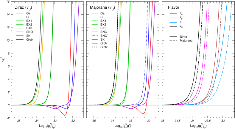
Figure 4: $\Delta\chi^{2}\equiv\chi^{2}(g_{s}^{N}g_{p}^{\nu_{U}})-\chi^{2}(g_{s}^{N}g_{p}^{\nu_{U}}=0)$ as a function of $g_{s}^{N}g_{p}^{\nu_{U}}$ for $m_{\phi}\ll 10^{-15}$ eV fixing all oscillation parameters (in particular $\Delta m^{2}_{21}$, $\theta_{12}$ and $\theta_{23}$) to their best-fit values. The left (central) panel show $\Delta\chi^{2}$ for each of the individual solar neutrino experiments for Dirac (Majorana) neutrinos and for the case of coupling to $\nu_{U}$. In the central panel SNO and SNO’ label the two variants of the SNO CC analysis for Majorana neutrinos (see text for details). The right panel show the global $\Delta\chi^{2}$ for four choices of the flavour dependence of the pseudoscalar-neutrino couplings; in particular, the black lines (coupling to $\nu_{U}$) for Dirac and Majorana cases coincide with the corresponding “Glob” ones in left and central panels, respectively.

The right panel illustrates the dependence of the combined bounds on the assumption for the neutrino flavour of the pseudscalar coupling for the four choices in Eq. (13). As seen the variation in the bounds is below $\mathcal{O}(10)$. As expected the difference is larger between coupling to $\nu_{e}$ and to $\nu_{\mu}$ (or $\nu_{\tau}$) because the coupling to $\nu_{e}$ has larger effect on $P_{ee}$ which gives the dominant contribution to the event rates in solar neutrino experiments. We notice in passing that the small variation between the bounds for couplings to $\nu_{\mu}$ and $\nu_{\tau}$ is dominantly due to the non-zero value of $\theta_{13}$.

Finally we list in table 1 the 90% CL (1 dof) bounds obtained from the global analysis of solar data in the two asymptotic regimes and for the four choices of flavour dependence after marginalization over the three relevant oscillation parameters $\Delta m^{2}_{21}$, $\theta_{12}$ and $\theta_{23}$.

		Global Solar $\nu$		Solar $\overline{\nu}_{e}$
		Dirac	Majorana	Majorana
	$a=e$	$1.5\times 10^{-34}$	$1.7\times 10^{-34}$	$1.1\times 10^{-33}$
$\big{|}g_{s}^{N}g_{p}^{\nu_{a}}\big{|}$	$a=\mu$	$3.6\times 10^{-34}$	$4.3\times 10^{-34}$	$7.6\times 10^{-34}$
for $m_{\phi}<10^{-16}$ eV	$a=\tau$	$3.6\times 10^{-34}$	$6.3\times 10^{-34}$	$7.9\times 10^{-34}$
	$a=U$	$7.6\times 10^{-35}$	$9.6\times 10^{-35}$	$3.2\times 10^{-34}$
	$a=e$	$1.3\times 10^{-31}$	$2.5\times 10^{-31}$	$1.9\times 10^{-31}$
$\frac{\left|g_{s}^{N}g_{p}^{\nu_{a}}\right|}{m_{\phi}\,/\,10^{-14}~{}\text{eV}^{2}}$	$a=\mu$	$2.0\times 10^{-31}$	$5.0\times 10^{-31}$	$2.5\times 10^{-31}$
for $m_{\phi}>10^{-14}$ eV	$a=\tau$	$2.0\times 10^{-31}$	$7.9\times 10^{-31}$	$2.5\times 10^{-31}$
	$a=U$	$6.3\times 10^{-32}$	$1.3\times 10^{-31}$	$7.0\times 10^{-32}$

Table 1: Bounds from the different analysis in the two asymptotic regimes, effective infinite interaction range and contact range respectively, and for the four choices of flavour dependence. For the global solar analysis the bounds sown are obtained at 90% CL (1 dof, two-sided), $\Delta\chi^{2}=2.71$. The bounds from the antineutrino flux constraint are obtained from the 90% CL experimental constraints in Eq. (16). See text for details.

Turning now to the bounds derived from the non observation of a flux of solar antineutrinos, we plot in the left panel in Fig. 5 a compilation of the model-independent limits on $\bar{\nu}_{e}$ flux of astrophysical origin as reported by KamLAND KamLAND:2021gvi , Borexino Borexino:2019wln and Super-Kamiokande Super-Kamiokande:2020frs ; Super-Kamiokande:2021jaq . In the same panel we also show the predicted flux in the presence of the helicty-flip potential for several model parameters. From the figure we see that the most stringent upper bounds on $\bar{\nu}_{e}$ come KamLAND KamLAND:2021gvi and Borexino Borexino:2019wln which constraint the $\bar{\nu}_{e}$ flux from the ${\mbox{}^{8}\text{B}}$ reaction by

KamLAND: $$\Phi^{{\mbox{}^{8}\text{B}}}_{\bar{\nu}_{e}} <\hphantom{0}60~{}\text{cm}^{-2}\,\text{s}^{-1}~{}\text{at 90\% CL for}~{}E_{\nu}>8.3~{}\text{MeV},$$ (14)

Borexino: $$\Phi^{{\mbox{}^{8}\text{B}}}_{\bar{\nu}_{e}} <138~{}\text{cm}^{-2}\,\text{s}^{-1}~{}\text{at 90\% CL for}~{}E_{\nu}>7.7~{}\text{MeV}.$$ (15)

which the experiments translated into a bound on the corresponding integrated oscillation probabilities

$$P(\nu_{e}\to\overline{\nu}_{e}) \equiv\frac{\int_{E_{\text{thres}}}\Phi_{{\mbox{}^{8}\text{B}}}(E_{\nu})\,\sigma(E_{\nu})\,P_{\nu_{eL}\to\overline{\nu}_{eR}}(E_{\nu})\,dE_{\nu}}{\int_{E_{\text{thres}}}\Phi_{{\mbox{}^{8}\text{B}}}(E_{\nu})\,\sigma(E_{\nu})\,dE_{\nu}}$$

$$\leq\begin{cases}3.5\times 10^{-5}&\text{for}~{}E_{\text{thres}}=8.3~{}\text{MeV}\\ 7.0\times 10^{-5}&\text{for}~{}E_{\text{thres}}=7.7~{}\text{MeV}\end{cases}$$ (16)

where we have used the normalization of the $\Phi_{{\mbox{}^{8}\text{B}}}(E_{\nu})$ of the latest version of the SSM B23Fluxes ; Magg:2022rxb which results in the slight difference in the bounds on the probabilities in Eq. (16) with respect to those quoted by the experimental collaborations.

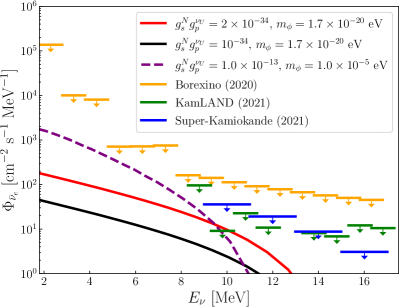
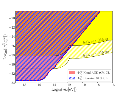
Figure 5: Left: Limits on $\bar{\nu}_{e}$ flux of astrophysical origin, as reported by KamLAND KamLAND:2021gvi , Borexino Borexino:2019wln and Super-Kamiokande Super-Kamiokande:2020frs ; Super-Kamiokande:2021jaq . For comparison, we show the expected solar $\bar{\nu}_{e}$ flux for several values of the model parameters as labeled in the figure. Right: Excluded region on the ($m_{\phi}$, $g_{s}^{N}g_{p}^{\nu_{U}}$) plane obtained for Majorana neutrinos obtained from the 90% CL constraint reported by KamLAND KamLAND:2021gvi and Borexino Borexino:2019wln , Eqs. (14) and (15) (see text for details). For comparison we show as yellow region the bounds on the product of couplings (see Sec. 4).

We show in the right panel of Fig. 5 the constraints on the model parameters obtained by the projection of the bounds in Eq. (16). For concreteness in this case we fix the oscillation parameters to their best-fit values, however as already noted the dependence of the bounds on the oscillation parameters is very mild within their allowed ranges from global oscillation analysis Esteban:2020cvm ; nufit-5.3 . We show the results for pseudoscalar coupling to $\nu_{U}$ but similar bounds apply to the other cases (see Table 1 for the results obtained with the different flavour assumptions in Eq. (13)). As seen from the figure the bounds imposed with KamLAND and Borexino constraints are very similar. In addition, we notice the expected mass independent asymptotic behavour for effectively infinite range interactions when $m_{\phi}\lesssim 10^{-16}$, as well as the dependence on $|g_{s}^{N}g_{p}^{\nu_{U}}|\,/\,m_{\phi}^{2}$ in the contact interaction regime for $m_{\phi}\gtrsim 10^{-14}$ eV.

4 Discussion

In this work we have shown that solar neutrinos are a powerful probe for interactions mediated by a spin-zero particle with pseudoscalar couplings to neutrinos and scalar coupling to the nucleons in the solar matter. We have evaluated the neutrino spin-flavour preceding potential generated by such interaction sourced by the nucleons in the Sun’s matter. This SFP potential presents the distinct feature of being most relevant for neutrinos with the lowest energies and therefore can be robustly constrained by a global analysis of solar oscillation results (in combination with KamLAND) in both cases of Dirac or Majorana neutrinos. In addition in the case of Majorana neutrinos the SFP potential also generates a flux of solar antineutrinos which is severely constrained from observations. Quantitatively our results show that, because of the distinctive energy dependence of the effect, the bounds obtained from the global analysis of solar neutrino data for both Dirac or Majorana neutrinos are comparable with those arising from the antineutrino constraints in the Majorana case.

We have focused on the limit of ultra light mediators for which the interaction length is comparable with the solar radius, finding that the bounds obtained go beyond existing constraints on the relevant couplings to nucleons and neutrinos. In brief, couplings of scalars to nucleons in this mass range are most strongly constrained by experiments testing the weak equivalence principle, in particular from the latest results by MICROSCOPE MICROSCOPE:2022doy for masses below $10^{-14}$ eV and by torsion balance experiments Schlamminger:2007ht (and also from fifth force searches, see Adelberger:2009zz for a compilation) in the range $10^{-14}$ eV to $10^{-6}$ eV. In what respects the pseudoscalar couplings to neutrinos in this mass range, they can be tested in a variety of probes, from laboratory experiments to effects in astrophysics and cosmology (for a recent review see Ref. Berryman:2022hds and references therein). Model independent bounds on couplings to neutrinos in this mediator mass range have been derived from kinematic and rate effects in meson, charge lepton, Higgs and Z decays Lessa:2007up ; Pasquini:2015fjv ; Berryman:2018ogk : $g_{p}^{\nu_{e}}\lesssim 3\times 10^{-3}$, $g_{p}^{\nu_{\mu}}\lesssim 10^{-3}$, $g_{p}^{\nu_{\tau}}\lesssim\text{few}\times 10^{-1}$, and from neutrinoless double beta decay $g_{p}^{\nu_{e}}\lesssim 10^{4}$–$10^{-5}$ Berryman:2022hds . Stronger but more model dependent constraints can be derived from effects in astrophysics (for example from supernova cooling Farzan:2002wx ) and cosmology. In particular the latest CMB data has been used to constraint couplings to very light (effectively massless) pseudoscalars $g_{p}^{\nu}\leq 7\times 10^{-7}$ Forastieri:2019cuf . For sake of comparison we show in Figs. 3 and 5 the range covered by the product of the bounds on $g_{s}^{N}$ from VEP constraints and the bound on $g_{p}^{\nu}$ from laboratory to CMB constraints. As seen in the figure the bounds derived in this work overcome the existing bounds obtained with constraints from laboratory experiments for mediator masses $m_{\phi}\lesssim 10^{-12}$ eV and with those from CMB for $m_{\phi}\lesssim 10^{-14}$ eV.

We finish by commenting on the possible relevance of these constraints for the proposed solution to the muon $g-2$ anomaly in Ref. Agrawal:2022wjm ; Davoudiasl:2022gdg which requires $g_{p}^{\mu}g_{s}^{N}\gtrsim 10^{-30}$. Taken at face values the constraints derived in this work rule out the proposed solution in the context of models in which the pseudoscalar coupling to the leptons of a given generation are related by symmetry. There is, however, a caveat. That conclusion is valid as long as the relation holds between the coupling $g_{p}^{\nu_{\mu}}$ in Eq. (1) and a muon coupling $g_{p}^{\mu}$ with interaction

$$i\,g_{p}^{\mu}\,\phi\,\bar{\mu}\gamma^{5}\mu$$ (17)

But pseudosecalar interactions for an on-shell fermion $\psi$ can equally be casted as

$$\tilde{g}^{\psi}\,\frac{\partial_{\mu}\phi}{f}\,\overline{\psi}\,\gamma^{\mu}\gamma^{5}\,\psi\,,$$ (18)

where $f$ sets the scale of the dimension-5 operator. For muons the relation between the couplings in Eq. (17) and (18) is $g_{p}^{\mu}=(2\,m_{\mu}/f)\,\tilde{g}_{p}^{\mu}$. For neutrinos the relation reads

$$\Big{(}U_{\text{vac}}^{\dagger}\,{g}_{p}^{\nu}\,U_{\text{vac}}\Big{)}_{ij}=\Big{(}U^{\dagger}_{\text{vac}}\,\tilde{g}_{p}^{\nu}\,U_{\text{vac}}\Big{)}_{ij}\frac{m_{i}+m_{j}}{f}$$ (19)

where $m_{i}$ are the neutrino masses. Thus if the symmetry relates the neutrino and muon couplings $\tilde{g}_{p}^{\nu_{\mu}}\sim\tilde{g}^{\mu}$ the bounds here derived, $g_{s}^{N}g^{\nu_{\mu}}\lesssim 10^{-34}$, would imply a weaker constraint, namely $g_{s}^{N}g^{\mu}\lesssim 10^{-34}\,m_{\mu}\big{/}m_{\nu_{h}}\sim 10^{-24}$ for the minimum possible value of the heavier neutrino mass $m_{\nu_{h}}\sim 0.05$ eV as required from oscillations.

Appendix A Derivation of the scalar-pseudoscalar potential

Our starting point is the well-known relation between the static potential generated by a non-relativistic source particle — here a nucleon $f$ located at $\vec{\rho}$ — felt by a probe particle — here a neutrino $\nu$ at position $\vec{x}$ — to the elastic scattering amplitude $\mathcal{M}$ of the process $\nu+f\to\nu+f$ as computed in QFT in momentum space

$$V(\vec{r}\equiv\vec{x}-\vec{\rho})=-\int d^{3}\vec{q}\,e^{i\vec{q}\cdot\vec{r}}\,\mathcal{M}(\vec{q})$$ (20)

with four-momentum transfer between the source particle and the neutrino given by $q\equiv(0,\vec{q})\equiv p^{\prime}-p$ where $p$ and $p^{\prime}$ are the neutrino four-momenta before and after the elastic scattering, which for a scalar-pseudoscalar interaction of a neutrino with mass $m$

$$\mathcal{L}=g_{s}^{f}\phi\bar{f}f+ig_{p}^{\nu}\phi\bar{\nu}\gamma^{5}\nu$$ (21)

reads

$$i\mathcal{M}=\frac{i(ig_{s}^{f})(-g_{p}^{\nu})}{q^{2}-m_{\phi}^{2}}\Big{[}\bar{u}_{r^{\prime}}^{f}(k)u_{r}^{f}(k)\Big{]}\Big{[}\bar{u}_{\lambda^{\prime}}^{\nu}(p^{\prime})\gamma^{5}u_{\lambda}^{\nu}(p)\Big{]}\,.$$ (22)

In writing Eq. (20) we are implicitly assuming the normaliation of the spinors to be one particle per unit volume for both nucleons and neutrinos. Explicitly, in the Dirac representation of the gamma matrices our choice for the spinor of fermion with four-momentum $(E,\vec{p})$ and spin state $s$ is

$$u_{s}(p)=\sqrt{\frac{E+m}{2E}}\begin{pmatrix}\chi_{s}\\ \frac{\vec{\sigma}\cdot\vec{p}}{E+m}\chi_{s}\end{pmatrix}$$ (23)

where $\chi_{s}$ are bi-spinors normalized as $\chi^{\dagger}_{s^{\prime}}\chi_{s}=\delta_{ss^{\prime}}$. With this choice, for the non-relativistic nucleons $\bar{u}_{r^{\prime}}^{f}(k^{\prime})u_{r}^{f}(k)=\delta_{rr^{\prime}}$, while for the neutrinos we can write

$$\bar{u}_{\lambda^{\prime}}^{\nu}(p^{\prime})\gamma^{5}u_{\lambda}^{\nu}(p)=\sqrt{\frac{E^{\prime}+m}{2E^{\prime}}}\sqrt{\frac{E+m}{2E}}\,\Big{(}\chi^{{\dagger}}_{\lambda^{\prime}}\vec{\sigma}\chi_{\lambda}\Big{)}\cdot\bigg{(}\frac{\vec{p}^{\prime}}{E+m}-\frac{\vec{p}}{E+m}\bigg{)}\,.$$ (24)

Expanding to the lowest non-vanishing order in $\vec{q}$ we find

$$\bar{u}_{\lambda^{\prime}}^{\nu}(p^{\prime})\gamma^{5}u_{\lambda}^{\nu}(p)=\frac{\chi^{{\dagger}}_{\lambda^{\prime}}\vec{\sigma}\chi_{\lambda}}{2E}\cdot\Big{[}\vec{q}-\Big{(}1-\frac{m}{E}\Big{)}(\hat{n}\cdot\vec{q})\,\hat{n}\Big{]},$$ (25)

where $\hat{n}$ is denoting the neutrino direction. Introducing (25) in Eq. (22) and evaluating the $\vec{q}$ integral in Eq. (20) one finds

$$V(\vec{r})=-\frac{g_{s}^{f}g_{p}^{\nu}}{4\pi E}\bigg{[}\vec{S}_{\lambda\lambda^{\prime}}-\Big{(}1-\dfrac{m}{E}\Big{)}(\vec{S}_{\lambda\lambda^{\prime}}\cdot\hat{n})\,\hat{n}\bigg{]}\cdot\vec{\nabla}_{r}\bigg{(}\frac{e^{-m_{\phi}r}}{r}\bigg{)}\,,$$ (26)

where we have defined $\vec{S}_{\lambda\lambda^{\prime}}\equiv\chi^{{\dagger}}_{\lambda^{\prime}}\,\vec{\sigma}\,\chi_{\lambda}$ as a spin-like vector quantity. In the non-relativistic limit $\vec{S}_{\lambda\lambda^{\prime}}$ corresponds to the spin of the neutrino, and Eq. (26) reduces to the well-known monompole-dipole potential Moody:1984ba

$$V(r)=g_{s}^{f}g_{p}^{\nu}\,\frac{\vec{\sigma}_{\nu}\cdot\hat{r}}{8\pi\,m_{\nu}}\,\bigg{[}\frac{m_{\phi}}{r}+\frac{1}{r^{2}}\bigg{]}\,e^{-m_{\phi}r}\,.$$ (27)

Conversely for relativistic neutrinos one can identify $\lambda$ with the helicity of the neutrino and using the explicit form of the spinors:

$$\vec{S}_{++}=-\vec{S}_{--}=\hat{n}\,,\qquad\vec{S}_{+-}\cdot\vec{\nabla}_{r}=\vec{S}_{-+}\cdot\vec{\nabla}_{r}=\Big{|}\hat{n}\times\vec{\nabla}_{r}\Big{|}\,,$$ (28)

we get

$$V(\vec{r})=-\frac{g_{s}^{f}\,g_{p}^{\nu}}{8\pi E}\,\bigg{[}\delta_{\lambda\neq\lambda^{\prime}}(\vec{\nabla}_{r})_{\perp}\pm\delta_{\lambda\lambda^{\prime}}\,\frac{m}{E}(\vec{\nabla}_{r})_{\parallel}\bigg{]}\,\bigg{(}\frac{e^{-m_{\phi}r}}{r}\bigg{)}$$ (29)

where

$$(\vec{\nabla}_{r})_{\parallel}\equiv(\hat{n}\cdot\vec{\nabla_{r}})\,\hat{n}\quad\text{and}\quad(\vec{\nabla}_{r})_{\perp}\equiv\vec{\nabla}_{r}-(\vec{\nabla}_{r})_{\parallel}$$ (30)

are the gradient operators along and perpendicular to the neutrino direction respectively. We notice that Eq. (29) displays the relativistic $1/\gamma=m/E$ factor suppression of the helicity-conserving potential in analogy with the well-known results for the potential generated by a magnetic field in the presence of a neutrino magnetic moment Akhmedov:1988hd ; Akhmedov:1988kih . Conversely the scalar-pseudoscalar interaction produces a helicity-flip potential which is proportional to the variation of the potential in the direction perpendicular to that of the neutrino propagation.

We are interested in taking the Sun as a source of the potential and for that we integrate Eq. (29) with the number density of nucleon $f$ at position $\vec{\rho}$ to obtain the potential at neutrino position $\vec{x}$ to be

$$V(\vec{x})=-\frac{g_{s}^{f}\,g_{p}^{\nu}}{8\pi\,E}\ \bigg{[}\delta_{\lambda\neq\lambda^{\prime}}(\vec{\nabla}_{x})_{\perp}\pm\delta_{\lambda\lambda^{\prime}}\,\frac{m}{E}(\vec{\nabla}_{x})_{\parallel}\bigg{]}\int N_{f}(\vec{\rho})\,\frac{e^{-m_{\phi}|\vec{\rho}-\vec{x}|}}{|\vec{\rho}-\vec{x}|}\,d^{3}\vec{\rho}\,.$$ (31)

where we have replaced $\vec{\nabla}_{r}$ with $-\vec{\nabla}_{\rho}=\vec{\nabla}_{x}$ because the position of the neutrino is fixed in the integral.

References

- (1) ATLAS, CMS collaboration, Precision tests of the Standard Model at the LHC with the ATLAS and CMS detectors, PoS FFK2019 (2020) 005.
- (2) ATLAS, CMS collaboration, Exotics and BSM in ATLAS and CMS (Non dark matter searches), PoS CORFU2019 (2020) 051.
- (3) C. Antel et al., Feebly-interacting particles: FIPs 2022 Workshop Report, Eur. Phys. J. C 83 (2023) 1122 [2305.01715].
- (4) S. Weinberg, A New Light Boson?, Phys. Rev. Lett. 40 (1978) 223.
- (5) F. Wilczek, Problem of Strong and Invariance in the Presence of Instantons, Phys. Rev. Lett. 40 (1978) 279.
- (6) R.D. Peccei and H.R. Quinn, CP Conservation in the Presence of Instantons, Phys. Rev. Lett. 38 (1977) 1440.
- (7) J. Preskill, M.B. Wise and F. Wilczek, Cosmology of the Invisible Axion, Phys. Lett. B 120 (1983) 127.
- (8) L.F. Abbott and P. Sikivie, A Cosmological Bound on the Invisible Axion, Phys. Lett. B 120 (1983) 133.
- (9) M. Dine and W. Fischler, The Not So Harmless Axion, Phys. Lett. B 120 (1983) 137.
- (10) Y. Chikashige, R.N. Mohapatra and R.D. Peccei, Are There Real Goldstone Bosons Associated with Broken Lepton Number?, Phys. Lett. B 98 (1981) 265.
- (11) G.B. Gelmini and M. Roncadelli, Left-Handed Neutrino Mass Scale and Spontaneously Broken Lepton Number, Phys. Lett. B 99 (1981) 411.
- (12) J.E. Moody and F. Wilczek, NEW MACROSCOPIC FORCES?, Phys. Rev. D 30 (1984) 130.
- (13) T. Aoyama et al., The anomalous magnetic moment of the muon in the Standard Model, Phys. Rept. 887 (2020) 1 [2006.04822].
- (14) S. Borsanyi et al., Leading hadronic contribution to the muon magnetic moment from lattice QCD, Nature 593 (2021) 51 [2002.12347].
- (15) Muon g-2 collaboration, Measurement of the Positive Muon Anomalous Magnetic Moment to 0.20 ppm, Phys. Rev. Lett. 131 (2023) 161802 [2308.06230].
- (16) R. Janish and H. Ramani, Muon g-2 and EDM experiments as muonic dark matter detectors, Phys. Rev. D 102 (2020) 115018 [2006.10069].
- (17) P. Agrawal, D.E. Kaplan, O. Kim, S. Rajendran and M. Reig, Searching for axion forces with precision precession in storage rings, Phys. Rev. D 108 (2023) 015017 [2210.17547].
- (18) H. Davoudiasl and R. Szafron, Muon g-2 and a Geocentric New Field, Phys. Rev. Lett. 130 (2023) 181802 [2210.14959].
- (19) L. Wolfenstein, Neutrino Oscillations in Matter, Phys. Rev. D 17 (1978) 2369.
- (20) S.P. Mikheev and A.Y. Smirnov, Resonance enhancement of oscillations in matter and solar neutrino spectroscopy, Sov. J. Nucl. Phys. 42 (1985) 913.
- (21) J. Grifols and E. Masso, Neutrino oscillations in the sun probe long range leptonic forces, Phys. Lett. B 579 (2004) 123 [hep-ph/0311141].
- (22) A.S. Joshipura and S. Mohanty, Constraints on flavor dependent long range forces from atmospheric neutrino observations at super-Kamiokande, Phys. Lett. B 584 (2004) 103 [hep-ph/0310210].
- (23) M.C. Gonzalez-Garcia, P.C. de Holanda, E. Masso and R. Zukanovich Funchal, Probing long-range leptonic forces with solar and reactor neutrinos, JCAP 0701 (2007) 005 [hep-ph/0609094].
- (24) H. Davoudiasl, H.-S. Lee and W.J. Marciano, Long-Range Lepton Flavor Interactions and Neutrino Oscillations, Phys. Rev. D 84 (2011) 013009 [1102.5352].
- (25) M.B. Wise and Y. Zhang, Lepton Flavorful Fifth Force and Depth-dependent Neutrino Matter Interactions, JHEP 06 (2018) 053 [1803.00591].
- (26) P. Coloma, M.C. Gonzalez-Garcia and M. Maltoni, Neutrino oscillation constraints on U(1)’ models: from non-standard interactions to long-range forces, JHEP 01 (2021) 114 [2009.14220]. [Erratum: JHEP 11, 115 (2022)].
- (27) A. Cisneros, Effect of neutrino magnetic moment on solar neutrino observations, Astrophys. Space Sci. 10 (1971) 87.
- (28) L.B. Okun, M.B. Voloshin and M.I. Vysotsky, Electromagnetic Properties of Neutrino and Possible Semiannual Variation Cycle of the Solar Neutrino Flux, Sov. J. Nucl. Phys. 44 (1986) 440.
- (29) L.B. Okun, M.B. Voloshin and M.I. Vysotsky, Neutrino Electrodynamics and Possible Effects for Solar Neutrinos, Sov. Phys. JETP 64 (1986) 446.
- (30) L.B. Okun, On the Electric Dipole Moment of Neutrino, Sov. J. Nucl. Phys. 44 (1986) 546.
- (31) M.B. Voloshin and M.I. Vysotsky, Neutrino Magnetic Moment and Time Variation of Solar Neutrino Flux, Sov. J. Nucl. Phys. 44 (1986) 544.
- (32) E.K. Akhmedov, Resonance enhancement of the neutrino spin precession in matter and the solar neutrino problem, Sov. J. Nucl. Phys. 48 (1988) 382.
- (33) C.-S. Lim and W.J. Marciano, Resonant Spin - Flavor Precession of Solar and Supernova Neutrinos, Phys. Rev. D 37 (1988) 1368.
- (34) M.C. Gonzalez-Garcia, M. Maltoni and J. Salvado, Testing matter effects in propagation of atmospheric and long-baseline neutrinos, JHEP 05 (2011) 075 [1103.4365].
- (35) M.C. Gonzalez-Garcia and M. Maltoni, Determination of matter potential from global analysis of neutrino oscillation data, JHEP 09 (2013) 152 [1307.3092].
- (36) I. Esteban, M.C. Gonzalez-Garcia, M. Maltoni, I. Martinez-Soler and J. Salvado, Updated constraints on non-standard interactions from global analysis of oscillation data, JHEP 08 (2018) 180 [1805.04530]. [Addendum: JHEP 12, 152 (2020)].
- (37) P. Coloma, M.C. Gonzalez-Garcia, M. Maltoni, J.a.P. Pinheiro and S. Urrea, Global constraints on non-standard neutrino interactions with quarks and electrons, JHEP 08 (2023) 032 [2305.07698].
- (38) P. Coloma, P. Coloma, M.C. Gonzalez-Garcia, M.C. Gonzalez-Garcia, M. Maltoni, M. Maltoni et al., Constraining new physics with Borexino Phase-II spectral data, JHEP 07 (2022) 138 [2204.03011]. [Erratum: JHEP 11, 138 (2022)].
- (39) E. Akhmedov and P. Martínez-Miravé, Solar flux: revisiting bounds on neutrino magnetic moments and solar magnetic field, JHEP 10 (2022) 144 [2207.04516].
- (40) B. Pontecorvo, Neutrino Experiments and the Problem of Conservation of Leptonic Charge, Sov. Phys. JETP 26 (1968) 984. [Zh. Eksp. Teor. Fiz.53,1717(1967)].
- (41) Z. Maki, M. Nakagawa and S. Sakata, Remarks on the unified model of elementary particles, Prog. Theor. Phys. 28 (1962) 870.
- (42) M. Kobayashi and T. Maskawa, CP Violation in the Renormalizable Theory of Weak Interaction, Prog. Theor. Phys. 49 (1973) 652.
- (43) P. Coloma and T. Schwetz, Generalized mass ordering degeneracy in neutrino oscillation experiments, Phys. Rev. D94 (2016) 055005 [1604.05772].
- (44) I. Esteban, M.C. Gonzalez-Garcia, M. Maltoni, T. Schwetz and A. Zhou, The fate of hints: updated global analysis of three-flavor neutrino oscillations, JHEP 09 (2020) 178 [2007.14792].
- (45) I. Esteban, M.C. Gonzalez-Garcia, M. Maltoni, T. Schwetz and A. Zhou, “NuFIT 5.3 (2024).” http://www.nu-fit.org.
- (46) B.T. Cleveland et al., Measurement of the solar electron neutrino flux with the Homestake chlorine detector, Astrophys. J. 496 (1998) 505.
- (47) F. Kaether, W. Hampel, G. Heusser, J. Kiko and T. Kirsten, Reanalysis of the GALLEX solar neutrino flux and source experiments, Phys. Lett. B685 (2010) 47 [1001.2731].
- (48) SAGE collaboration, Measurement of the solar neutrino capture rate with gallium metal. III: Results for the 2002--2007 data-taking period, Phys. Rev. C80 (2009) 015807 [0901.2200].
- (49) Super-Kamiokande collaboration, Solar neutrino measurements in Super-Kamiokande-I, Phys. Rev. D73 (2006) 112001 [hep-ex/0508053].
- (50) Super-Kamiokande collaboration, Solar neutrino measurements in Super-Kamiokande-II, Phys. Rev. D78 (2008) 032002 [0803.4312].
- (51) Super-Kamiokande collaboration, Solar neutrino results in Super-Kamiokande-III, Phys. Rev. D83 (2011) 052010 [1010.0118].
- (52) Super-Kamiokande collaboration, Solar neutrino measurements using the full data period of Super-Kamiokande-IV, 2312.12907.
- (53) SNO collaboration, Measurement of the nu/e and total B-8 solar neutrino fluxes with the Sudbury Neutrino Observatory phase I data set, Phys. Rev. C75 (2007) 045502 [nucl-ex/0610020].
- (54) SNO collaboration, Electron energy spectra, fluxes, and day-night asymmetries of B-8 solar neutrinos from the 391-day salt phase SNO data set, Phys. Rev. C72 (2005) 055502 [nucl-ex/0502021].
- (55) SNO collaboration, An Independent Measurement of the Total Active 8B Solar Neutrino Flux Using an Array of 3He Proportional Counters at the Sudbury Neutrino Observatory, Phys. Rev. Lett. 101 (2008) 111301 [0806.0989].
- (56) Borexino collaboration, Precision measurement of the 7Be solar neutrino interaction rate in Borexino, Phys. Rev. Lett. 107 (2011) 141302 [1104.1816].
- (57) Borexino collaboration, Measurement of the solar 8B neutrino rate with a liquid scintillator target and 3 MeV energy threshold in the Borexino detector, Phys. Rev. D82 (2010) 033006 [0808.2868].
- (58) Borexino collaboration, First Simultaneous Precision Spectroscopy of , 7Be, and Solar Neutrinos with Borexino Phase-II, Phys. Rev. D 100 (2019) 082004 [1707.09279].
- (59) BOREXINO collaboration, Improved Measurement of Solar Neutrinos from the Carbon-Nitrogen-Oxygen Cycle by Borexino and Its Implications for the Standard Solar Model, Phys. Rev. Lett. 129 (2022) 252701 [2205.15975].
- (60) KamLAND collaboration, Reactor On-Off Antineutrino Measurement with KamLAND, Phys. Rev. D88 (2013) 033001 [1303.4667].
- (61) Daya Bay collaboration, Precision measurement of reactor antineutrino oscillation at kilometer-scale baselines by Daya Bay, 2211.14988.
- (62) KamLAND collaboration, Limits on Astrophysical Antineutrinos with the KamLAND Experiment, Astrophys. J. 925 (2022) 14 [2108.08527].
- (63) Borexino collaboration, Search for low-energy neutrinos from astrophysical sources with Borexino, Astropart. Phys. 125 (2021) 102509 [1909.02422].
- (64) Super-Kamiokande collaboration, Search for solar electron anti-neutrinos due to spin-flavor precession in the Sun with Super-Kamiokande-IV, 2012.03807.
- (65) Super-Kamiokande collaboration, Diffuse supernova neutrino background search at Super-Kamiokande, Phys. Rev. D 104 (2021) 122002 [2109.11174].
- (66) Y. Herrera and A. Serenelli, Standard Solar Models B23 / SF-III, 2023. ZENODO, https://doi.org/10.5281/zenodo.10174170.
- (67) E. Magg et al., Observational constraints on the origin of the elements - IV. Standard composition of the Sun, Astron. Astrophys. 661 (2022) A140 [2203.02255].
- (68) MICROSCOPE collaboration, MICROSCOPE Mission: Final Results of the Test of the Equivalence Principle, Phys. Rev. Lett. 129 (2022) 121102 [2209.15487].
- (69) J. Bergé, P. Brax, G. Métris, M. Pernot-Borràs, P. Touboul and J.-P. Uzan, MICROSCOPE Mission: First Constraints on the Violation of the Weak Equivalence Principle by a Light Scalar Dilaton, Phys. Rev. Lett. 120 (2018) 141101 [1712.00483].
- (70) P. Touboul et al., MICROSCOPE Mission: First Results of a Space Test of the Equivalence Principle, Phys. Rev. Lett. 119 (2017) 231101 [1712.01176].
- (71) S. Schlamminger, K.Y. Choi, T.A. Wagner, J.H. Gundlach and E.G. Adelberger, Test of the equivalence principle using a rotating torsion balance, Phys. Rev. Lett. 100 (2008) 041101 [0712.0607].
- (72) E. Adelberger, J. Gundlach, B. Heckel, S. Hoedl and S. Schlamminger, Torsion balance experiments: A low-energy frontier of particle physics, Prog. Part. Nucl. Phys. 62 (2009) 102.
- (73) J.M. Berryman et al., Neutrino self-interactions: A white paper, Phys. Dark Univ. 42 (2023) 101267 [2203.01955].
- (74) A.P. Lessa and O.L.G. Peres, Revising limits on neutrino-Majoron couplings, Phys. Rev. D 75 (2007) 094001 [hep-ph/0701068].
- (75) P.S. Pasquini and O.L.G. Peres, Bounds on Neutrino-Scalar Yukawa Coupling, Phys. Rev. D 93 (2016) 053007 [1511.01811]. [Erratum: Phys.Rev.D 93, 079902 (2016)].
- (76) J.M. Berryman, A. De Gouvêa, K.J. Kelly and Y. Zhang, Lepton-Number-Charged Scalars and Neutrino Beamstrahlung, Phys. Rev. D 97 (2018) 075030 [1802.00009].
- (77) Y. Farzan, Bounds on the coupling of the Majoron to light neutrinos from supernova cooling, Phys. Rev. D 67 (2003) 073015 [hep-ph/0211375].
- (78) F. Forastieri, M. Lattanzi and P. Natoli, Cosmological constraints on neutrino self-interactions with a light mediator, Phys. Rev. D 100 (2019) 103526 [1904.07810].
- (79) E.K. Akhmedov and M.Y. Khlopov, Resonant Amplification of Neutrino Oscillations in Longitudinal Magnetic Field, Mod. Phys. Lett. A 3 (1988) 451.
- (80) E.K. Akhmedov and M.Y. Khlopov, Resonant Enhancement of Neutrino Oscillations in Longitudinal Magnetic Field, Sov. J. Nucl. Phys. 47 (1988) 689.