Barren plateaus are swamped with traps

Abstract

Two main challenges preventing efficient training of variational quantum algorithms and quantum machine learning models are local minima and barren plateaus. Typically, barren plateaus are associated with deep circuits, while shallow circuits have been shown to suffer from suboptimal local minima. We point out a simple mechanism that creates exponentially many poor local minima specifically in the barren plateau regime. These local minima are trivial solutions, optimizing only a few terms in the loss function, leaving the rest on their barren plateaus. More precisely, we show the existence of approximate local minima, optimizing a single loss term, and conjecture the existence of exact local minima, optimizing only a logarithmic fraction of all loss function terms. One implication of our findings is that simply yielding large gradients is not sufficient to render an initialization strategy a meaningful solution to the barren plateau problem.

I Introduction

Variational quantum algorithms (VQAs) [1] and a closely related field of quantum machine learning (QML) [2, 3] are still the leading paradigms for quantum computing in the NISQ era [4, 5, 6]. They are considered a natural generalization of the classical neural networks, with the potential to leverage the power of quantum information processing. While VQAs and QML are expected to surpass classical models in certain aspects, only a few theoretical results concerning their performance are available up to date.

One of the key obstacles facing VQAs and QML models [7, 8] is trainability. Loss functions in classical deep neural networks are known to be highly non-convex [9]. Nevertheless, they usually can be optimized with surprising efficiency by gradient-based methods, i.e. they are trainable. Unfortunately, the trainability of VQAs appears to be a qualitatively harder problem. Two main issues are poor local minima (LM) and barren plateaus (BPs). It is possible to construct VQAs that are provably NP-hard to optimize owing to the exponential number of LM in the loss landscape [10]. More importantly, the domination of poor LM appears to be a generic [11, 12], rather than a fine-tuned [10, 13] property.

BPs, as first pointed out in Ref. [14] and elaborated in many subsequent works (see Ref. [15] for a succinct recent review), describe the situation where the loss function has exponentially small (in the number of qubits $n$) variance. In other words, the loss landscape is basically flat with exponential precision everywhere, possibly except for a parameter region of an exponentially small volume. The presence of BPs is a generic property, manifesting the curse of dimensionality associated with the exponentially large Hilbert space. The most important cause of BPs is expressivity of a VQA, which generically appears for sufficiently deep $poly(n)$ circuits. Hence, BPs are often considered to be a problem of deep circuits. In contrast, shallow $poly(log(n))$ quantum circuits can be free of BPs, but have been shown to suffer from poor LM [11, 12].

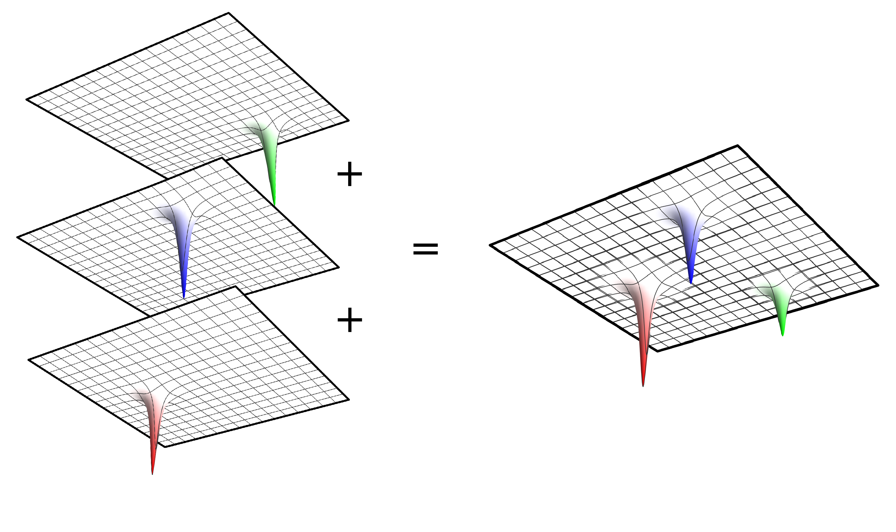
Figure 1: Schematic illustration of the main idea. When the loss functions corresponding to the individual observables are highly concentrated (left), their respective local minima are likely to remain the local minima of the total loss function (right).

Here we argue that a very general class of VQAs contains exponentially many LM of a particular type in the BP regime as well. The very possibility of LM coexisting with BP is not new. Theoretically [16, 11, 12] and empirically [17, 18, 19, 20], LM have been shown to disappear only in the in overparameterized circuits, which typically implies exponential depth far beyond the onset of BPs. However, the structure of these LM is not well-understood, for instance [11] suggested that they might be mostly represented by exponentially shallow bumps. In contrast, here we show that there can be exponentially many LM with sufficiently large (absolute) loss values, accompanied by sufficiently large gradients in their vicinity.

The basic idea is simple and can be sketched as follows. An observable $O$ in a VQA is typically a sum of simpler operators $O=\sum_{i}O_{i}$. To each of these we can associate a separate loss function $L_{i}(\boldsymbol{\phi})$, so that the full loss function is their sum $L(\boldsymbol{\phi})=\sum_{i}L_{i}(\boldsymbol{\phi})$, where $\boldsymbol{\phi}$ is a vector of VQA’s parameters. If the full loss function $L(\boldsymbol{\phi})$ has a BP, each of the contributing terms $L_{i}(\boldsymbol{\phi})$ has a BP as well.

Then, any point $\boldsymbol{\phi}_{i}$ that is a local minimum for some particular $L_{i}$, is likely to be a local minimum for the total loss function $L$ as well, simply because the contribution of the other terms $L_{j\neq i}$ is exponentially close to zero over most of the parameter space, see Fig. 1 for an illustration. Typically, a single term $L_{i}$ captures only a tiny bit of information about the original problem, e.g. a single interaction term in a molecular Hamiltonian or a single constraint in a combinatorial optimization problem. Hence, such points, which we refer to as siloed LM, are expected to yield very poor solutions.

To make this idea precise, we need to (i) be able to characterize LM of individual loss functions $L_{i}$ and (ii) prove that LM of different terms are sufficiently uncorrelated to not interfere with each other. In this work, we focus on a class of VQA we refer to as Clifford VQAs, which only involve constant Clifford gates, Pauli observables, and parameterized Pauli rotations. Clifford VQAs provide us with sufficient control to make a precise argument and at the same time, they capture most of ansatz structures appearing in practice such as QAOA [21], the majority of hardware-efficient circuits [22] and VQE [23]. We also discuss whether our conclusions are likely to apply to other types of VQAs in Sec. V.

In practice, the behavior depicted in Fig. 1, gives an oversimplified picture in most cases. In the Clifford VQA setting, we find that the LM of individual Pauli terms are not isolated points, but rather high-dimensional surfaces, as illustrated in Fig. 3, and discussed in detail later. We will show that points on these critical surfaces typically are approximate LM (up to exponentially vanishing gradients), and argue that intersection of ${\cal O}(\log(n))$ such surfaces are exact LM. However, at the beginning, we encourage the reader to refer to the more intuitive picture sketched in Fig. 1.

Our findings add to the bundle of challenges that need to be addressed when designing and training VQAs. There are two primary ways to deal with the BP problem. The first is to use ansatz structures that are free of BPs by design, such as shallow local circuits [24], circuits with polynomial dynamical Lie algebras [16, 25] or special symmetry structure [26, 27]. However, a growing body of evidence, distilled in recent work [28], implies that the very same properties that prevent BPs make the relevant VQAs classically simulable. Another approach is to use specific parameter initializations that, while not eliminating the BPs, prevent the training from starting there. However, most of these initialization strategies rely on the initial quantum circuit being close to the identity [29, 30, 31, 32]. It is not clear a priori whether such initializations allow the optimization to cross over into the deep circuit regime. Other initialization strategies exits that target deeps circuits [33], or even specifically Clifford circuits [34]. However, in all those cases, the possibility to end up in a poor LM should not be ignored. Hence, we argue that an initialization leading to large gradients is not synonymous with solving the BP problem.

II Barren plateaus

II.1 Definition and origins

A VQA is defined by an initial state $\rho$, a parameterized quantum circuit $U(\boldsymbol{\phi})$, and an observable $O$, with the loss function given by the expectation value

$$L(\boldsymbol{\phi})=\operatorname{Tr}\left[\rho\,U^{\dagger}(\boldsymbol{\phi})\,O\,U(\boldsymbol{\phi})\right]\ ,$$ (1)

with $\boldsymbol{\phi}=(\phi_{k})$ being a vector of parameters. The loss function $L(\boldsymbol{\phi})$ is said to have a BP if its values are exponentially concentrated around the mean $\mathbb{E}[L]$, i.e. when the variance of the loss function, defined by

$$\mathbb{V}[L]=\mathbb{E}\left[\left(L(\boldsymbol{\phi})-\mathbb{E}[L]\right)^{2}\right]\ ,$$ (2)

vanishes exponentially with the number of qubits $\mathbb{V}[L]={\cal O}(b^{-n})$ for some $b>1$. In the standard setting $b=2$, which is directly related to the dimension of the $n$-qubit Hilbert space. For functions $F(\boldsymbol{\phi})$ periodic with respect to each variable $\phi_{k}$, which is the most common case in practice, expectation values are calculated as $\mathbb{E}[F]=\int_{0}^{2\pi}\prod_{k}\frac{d\phi_{k}}{2\pi}\,\,F(\boldsymbol{\phi})$.

We note that though originally BPs were defined by vanishing gradients rather than the concentration of loss function [14], these conditions are in fact equivalent [35, 36], and loss concentration is usually a more convenient diagnostic tool. Still, some of our arguments will rely on the gradient concentration. For a loss function $L(\boldsymbol{\phi})$ with variance $\mathbb{V}[L]=\mathcal{O}(b^{-n})$ and for any $\epsilon$, the concentration result can be stated formally using Chebyshev’s inequality

$$\Pr\left[\Big{|}L-\mathbb{E}[L]\Big{|}>\epsilon\right]\leq\mathcal{O}\left(\epsilon^{-2}b^{-n}\right)\ .$$ (3)

Four main sources of BPs have been identified in the literature.

• Circuit expressivity. When the parameterized quantum circuit defining the VQA furnishes an approximate unitary 2-design, $L$ suffers from a BP [14, 37]. Typically, local circuits beyond linear depth $d={\cal O}(n)$ are sufficient to qualify for 2-designs [38, 39], while the logarithmic depth $d={\cal O}(\log n)$ circuits are not.

• Non-locality of the observable. VQAs with shallow local circuits can have a BP if the observable $O$ is sufficiently non-local [40, 41], which is the case in many of the proposed VQA applications such as, for example, quantum compiling [42, 43] or autoencoders [44].

• Entanglement of the initial state. BP can arise in VQAs with sufficiently entangled initial states $\rho$, which is common in quantum machine learning and quantum chemistry [45, 7, 46, 47].

• Noise. Sufficiently strong noise also generically leads to BPs [48, 49, 50, 51]. Noise-induced BPs are qualitatively different from the rest, as the noise tends to flatten the loss landscape completely, instead of concentrating good solutions in a small parameter region.

Interestingly, our argument will be sufficiently general and apply to any source of the BP (except for the noise), so that the classification above will be useful to interpret the results, but not necessary to derive them. At the same time, we will heavily rely on the properties of a specific class of VQAs, that we now introduce.

II.2 Clifford VQAs

The class of VQAs we consider here restricts the initial state $\rho$ to be a stabilizer state, the observable $O$ to be a sum of $poly(n)$ Pauli stings $O=\sum_{i}c_{i}P_{i}$ with real coefficients $c_{i}$, and the circuit $U(\boldsymbol{\phi})$ to consist only of the constant Clifford gates and parametric Pauli rotation gates $e^{-\imath P_{k}\phi_{k}/2}$. Generators of the parametric gates $P_{k}$ and Pauli observables $P_{i}$ may or may not be related. We will refer to such VQAs as Clifford VQAs. We also assume that there are no correlated parameters, i.e. that all angles $\phi_{k}$ are independent, and that there are at most $poly(n)$ parameters in total.

Denote by $|\boldsymbol{\phi}|$ the total number of parameters in the circuit, by $\boldsymbol{\phi_{\mathcal{C}}}$ a discrete set $\boldsymbol{\phi_{\mathcal{C}}}=\{0,\pi/2,\pi,3\pi/2\}^{|\boldsymbol{\phi}|}$ (the set of all $4^{|\boldsymbol{\phi}|}$ combinations obtained by setting each component of $\boldsymbol{\phi}$ to either $0,\pi/2,\pi$ or $3\pi/2$). The key technical fact allowing to derive most of our quantitative results is the following

Lemma 1 (Averaging over Clifford points)

Let $F(\boldsymbol{\phi})$ be a trigonometric polynomial of degree at most two with respect to each angle $\phi_{k}$. Then,

$$\mathbb{E}[F]=\frac{1}{4^{|\boldsymbol{\phi}|}}\sum_{\boldsymbol{\phi}_{c}\in\boldsymbol{\phi_{\mathcal{C}}}}F(\boldsymbol{\phi}_{c})\ .$$ (4)

The simple proof, as well as a precise definition of degree two trigonometric polynomial, is found in App. A.1. With our definition of a Clifford VQA, and in the absence of correlated parameters, both $L(\boldsymbol{\phi})$ and $L^{2}(\boldsymbol{\phi})$ satisfy conditions of this Lemma, a simple fact made explicit in App. A.2. This allows expressing variance (2) as the sum over the discrete set of points $\boldsymbol{\phi_{\mathcal{C}}}$. For $\boldsymbol{\phi}_{c}\in\boldsymbol{\phi_{\mathcal{C}}}$ all the Pauli rotation gates in $U(\boldsymbol{\phi}_{c})$ become Clifford operators and $U(\boldsymbol{\phi}_{c})$ becomes a Clifford circuit, hence we refer to $\boldsymbol{\phi_{\mathcal{C}}}$ as the Clifford points.

Now let us consider the case where the observable is a single Pauli string $P$. Then, the value of the loss function at a Clifford point $\boldsymbol{\phi}_{c}$ can be either $\pm 1$ or $0$. This is because at a Clifford point $U^{\dagger}(\boldsymbol{\phi}_{c})PU(\boldsymbol{\phi}_{c})$ is again a Pauli string, and its expectation value in the stabilizer state $\rho$ is either $0$ or $\pm 1$. This basic fact allows us to derive the following

Theorem 1 (Concentration at Clifford points)

Let the loss function $L$ of a Clifford VQA have a BP with $\mathbb{V}[L]={\cal O}(b^{-n})$. Then, for a randomly sampled Clifford point $\boldsymbol{\phi}_{c}\in\boldsymbol{\phi_{\mathcal{C}}}$, the probability that $L(\boldsymbol{\phi}_{c})$ is not equal to its expected value vanishes exponentially

$$\Pr(|L(\boldsymbol{\phi}_{c})-\mathbb{E}[L]|>0)={\cal O}(b^{-n})\ .$$ (5)

Similarly, any gradient component or Hessian entry is zero with probability exponentially close to one

$$\Pr(|\nabla_{\phi_{k}}L(\boldsymbol{\phi}_{c})|>0)={\cal O}(b^{-n}),$$ (6)

$$\Pr(|\nabla_{\phi_{k}}\nabla_{\phi_{l}}L(\boldsymbol{\phi}_{c})|>0)={\cal O}(b^{-n})\ .$$ (7)

The proof if straightforward. For simplicity, and without the loss of generality, we set $\mathbb{E}[L]=0$, so that the variance is given by $\mathbb{V}[L]=\mathbb{E}[L^{2}]$ (see App. A.3 for justification of this assumption). First, consider the case of a single Pauli observable $P_{i}$. As explained above, the value of the corresponding loss function at the Clifford points is either $L_{i}^{2}=1$ or $L_{i}^{2}=0$. Therefore, according to Lemma 1, the variance

$$\mathbb{V}[L_{i}]=\frac{1}{4^{|\boldsymbol{\phi}|}}\sum_{\boldsymbol{\phi}_{c}\in\boldsymbol{\phi_{\mathcal{C}}}}L_{i}^{2}(\boldsymbol{\phi}_{c})$$ (8)

simply counts the number of non-zero values at Clifford points normalized by the total number of Clifford points. If $L_{i}$ has a BP, this variance, and hence the proportion of the Clifford points with non-zero value, is exponentially small, leading to (5). Clearly, replacing a single Pauli observable $P_{i}$ by a $poly(n)$ sum of Pauli strings $O=\sum_{i}c_{i}P_{i}$ can not overcome the exponential concentration. The reasoning extends to the derivatives as well. For instance, using the parameter-shift rule [52, 53] the gradient can be expressed as

$$\nabla_{\phi_{k}}L(\boldsymbol{\phi})=\frac{1}{2}L\left(\boldsymbol{\phi}+\frac{\pi}{2}\boldsymbol{e}_{k}\right)-\frac{1}{2}L\left(\boldsymbol{\phi}-\frac{\pi}{2}\boldsymbol{e}_{k}\right)\ ,$$ (9)

where $\boldsymbol{e}_{k}$ is a unit vector in the direction of $\phi_{k}$. Each of the two terms contributing to the gradient (i) has a BP (ii) assumes a discrete set of values $\pm\frac{1}{2},0$ at Clifford points and (iii) satisfies conditions of Lemma 1. Hence, their sum will inherit all these properties and then Eq. (6) can be deduced in the same way as Eq. (5) (note that $\mathbb{E}[\nabla_{\phi_{k}}L]=0$ is manifest from (9)). Similar reasoning applies to the Hessian components, and we will not spell it out.

The main conclusion of this section is as follows. Almost by definition, randomly sampling the parameters of a VQA suffering from a BP leads to exponentially small loss value, with probability exponentially close to one. We have shown that for a Clifford VQA random sampling of a Clifford point leads to loss being exactly zero, with probability exponentially close to one. Moreover, the same applies to any finite derivative of the loss function.

III Traps in barren plateaus

III.1 Loss landscapes of single Pauli terms

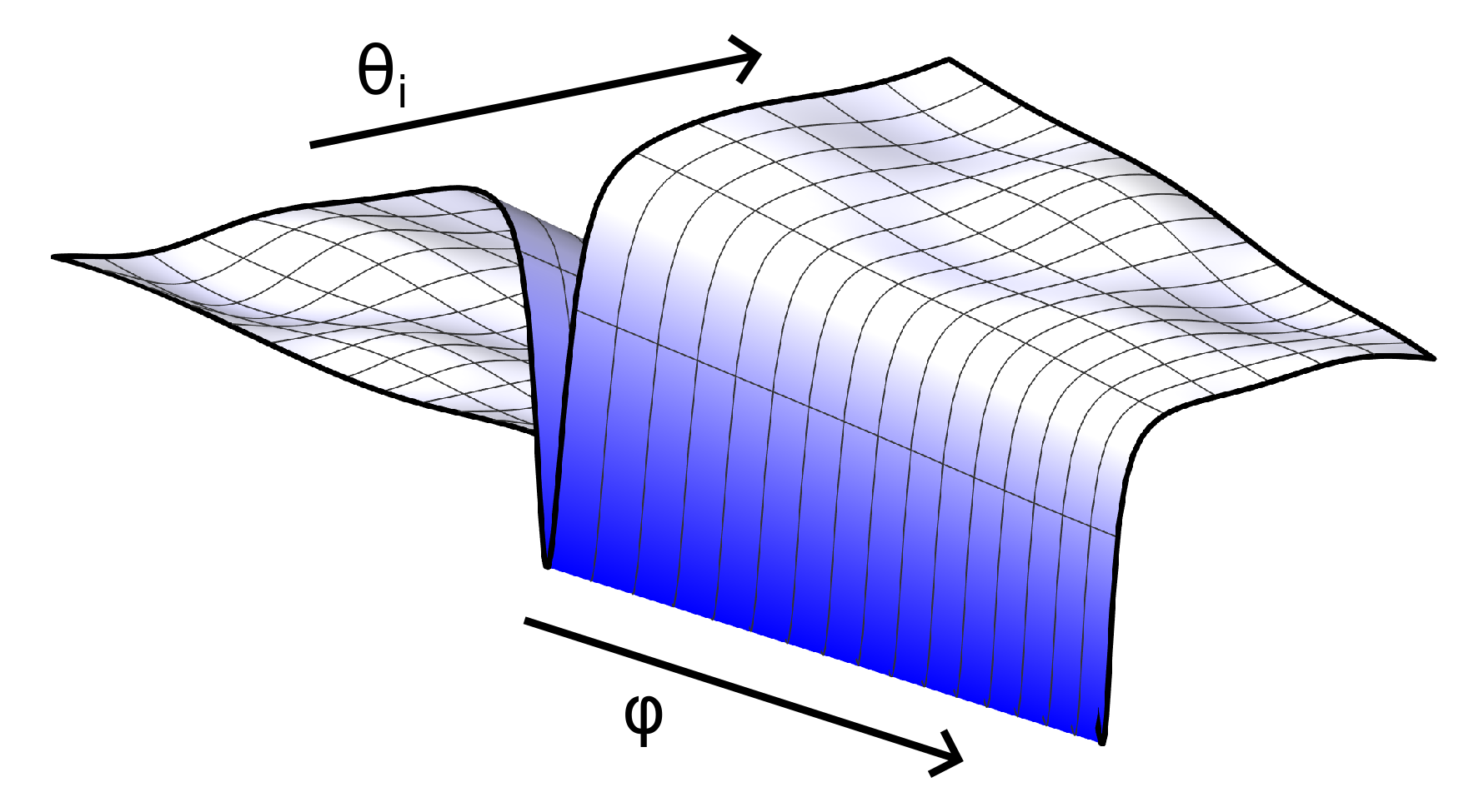
Figure 2: Local structure of the critical surface for a single Pauli observable.

We begin by discussing the structure of the loss landscapes $L_{i}$, involving a single Pauli observable $P_{i}$. One simple observation is that any point $\boldsymbol{\phi}_{i}$ yielding $L_{i}(\boldsymbol{\phi}_{i})=-|c_{i}|$ is a global minimum of $L_{i}(\boldsymbol{\phi})$, because the expectation value of $P_{i}$ is bounded between $-1$ and $+1$. Another point, which is less obvious, is that LM of $L_{i}$ almost never are isolated points, but rather hypersurfaces of high dimension. In other words, the parameter vector $\boldsymbol{\phi}_{i}$ typically admits a split $\boldsymbol{\phi}_{i}$ into fixed $\boldsymbol{\theta}_{i}$ and free $\boldsymbol{\varphi}$ components

$$\boldsymbol{\phi}_{i}=(\boldsymbol{\theta}_{i},\boldsymbol{\varphi}),$$ (10)

such that changing any of the parameters $\boldsymbol{\theta}_{i}$ leads away from the critical surface, while changing $\boldsymbol{\varphi}$ has no effect, i.e. $L_{i}(\boldsymbol{\theta}_{i},\boldsymbol{\varphi})=-|c_{i}|$ for any choice of $\boldsymbol{\varphi}$ (not necessarily Clifford). This is illustrated in Fig. 2. We will refer to $\boldsymbol{\varphi}$ as null directions. Note that $L_{i}$ needs to be independent of $\boldsymbol{\varphi}$ only when $\boldsymbol{\theta}_{i}$ are fixed, i.e. only the bottom of the gorge needs to be flat.

An easy case showing that null directions exist is a VQA with local observables. Then, all the parameters in $\boldsymbol{\phi}_{i}$, whose generators lie outside the observable’s lightcone, are trivially null directions. However, null directions appear much more generally. To see this, fix all parameters $\boldsymbol{\phi}$ to their values implied by $\boldsymbol{\phi}_{i}$, except for a single angle $\phi_{k}$. As a function of $\phi_{k}$, the circuit has the form $U(\phi_{k})=C_{L}e^{-iP_{k}\phi_{k}/2}C_{R}$ with both $C_{L}$ and $C_{R}$ being Clifford gates (which are combinations of the original Clifford gates, and Clifford gates resulted from fixing all the other parameterized gates to their Clifford values). The loss function then is

$$L_{i}(\phi_{k})=\operatorname{Tr}\left[\rho\,\,C_{R}^{\dagger}e^{iP_{k}\phi_{k}/2}C_{L}^{\dagger}P_{i}C_{L}e^{-iP_{k}\phi_{k}/2}C_{R}\right]\ .$$ (11)

If the generator $P_{k}$ commutes with the Pauli operator $C_{L}^{\dagger}P_{i}C_{L}$, then $L_{i}(\phi_{k})$ in fact does not depend on $\phi_{k}$ and hence $\phi_{k}$ is a null direction. If $P_{k}$ is outside of $P_{i}$’s lightcone, these operators necessarily commute. However, even when the lightcones of $P_{i}$ and $P_{k}$ intersect, we expect them to commute roughly half of the times, simply because two random Pauli strings sharing qubits have one half probability of commuting. Hence, in a generic case, we expect all the parameters outside the lightcone of $P_{i}$, and roughly half of the parameters within, to be null directions for $L_{i}$, so that $|\boldsymbol{\varphi}|\geq|\boldsymbol{\phi}|/2$. As shown in App. B.1 it is possible to construct loss functions $L_{i}$ that have few to no null directions at their critical points, but such examples are arguably contrived.

Therefore, we need to update our initial sketch in Fig. 1 replacing localized sharp peaks with narrow gorges, see Fig. 3. This figure suggests the existence of two types of LM, those that belong to a single gorge and optimize a single term in the loss function, and those that lie on the intersection of several gorges and optimize several terms. We will discuss both types in turn.

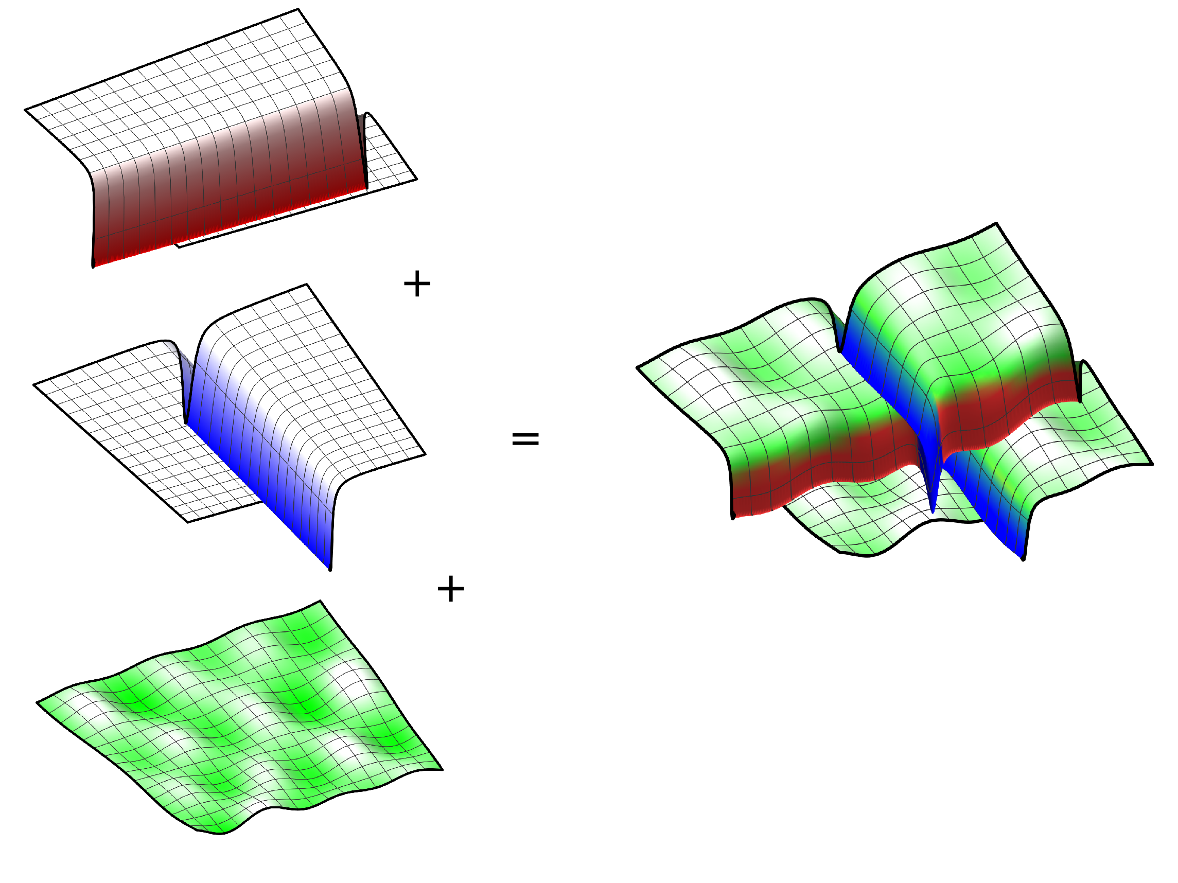
Figure 3: Loss gorges corresponding to individual Pauli terms, and their interaction.

III.2 Approximate local minima

We are now ready to quantitatively argue that quite generally, a random point $\boldsymbol{\phi}_{i}$, which is a global minimum for one of the Pauli observables $L_{i}$, is exponentially likely to be an approximate local minimum for the full loss function $L$. The intuitive definition of an approximate local minimum $\boldsymbol{\phi}_{*}$ is that of a point, where it is not possible to meaningfully improve the value of the loss function $L(\boldsymbol{\phi}_{*})$ by any small perturbation. More precisely, following the mathematical literature (see e.g. [54]) we say that $\boldsymbol{\phi}_{*}$ is an $\epsilon$-approximate critical point of $L(\boldsymbol{\phi})$, if all gradient components at $\boldsymbol{\phi}_{*}$ are bounded by $|\nabla_{\phi_{k}}L(\boldsymbol{\phi}_{*})|\leq\epsilon$. If, furthermore, the smallest eigenvalue $\lambda_{\rm min}$ of the Hessian $\nabla^{2}L(\boldsymbol{\phi}_{*})$ satisfies $\lambda_{\min}\geq-\sqrt{\epsilon}$, we call $\boldsymbol{\phi}_{*}$ an $\epsilon$-approximate local minimum.

Our argument is based on a simple variation of the idea presented in the introduction. Let us divide the loss function into $L_{i}$, the term that was specifically optimized by the choice of $\boldsymbol{\phi}_{i}$, and the rest of the terms $R_{i}(\boldsymbol{\phi})=L(\boldsymbol{\phi})-L_{i}(\boldsymbol{\phi})=\sum_{j\neq i}L_{j}(\boldsymbol{\phi})$. Assuming that $R_{i}(\boldsymbol{\phi})$ is in some sense independent of $L_{i}(\boldsymbol{\phi})$, the vicinity of the point $\boldsymbol{\phi}_{i}$ is likely to be a generic region for $R_{i}$, and lie on its BP. Hence, adding $R_{i}$ could only change the value of $L_{i}$ by an exponentially small margin, and at most turn $\boldsymbol{\phi}_{i}$ into an $\epsilon$-approximate local minimum instead of an exact one. This is illustrated in Fig. 4. The technical condition leading to the desired notion of independence between $L_{i}$ and $R_{i}$ is the requirement that $R_{i}(\boldsymbol{\theta}_{i},\boldsymbol{\varphi})$ has a BP with respect to the null directions of $L_{i}$. This is formalized by

Theorem 2 (Approximate local minima)

Let $L(\boldsymbol{\phi})=\sum_{j}L_{j}(\boldsymbol{\phi})$ be a loss function of a Clifford VQA having a BP, and a Clifford point $\boldsymbol{\phi}_{i}$ be a local minimum of some $L_{i}$ with $L_{i}(\boldsymbol{\phi}_{i})=-|c_{i}|$. Denote the rest of the terms in the loss function by $R_{i}(\boldsymbol{\phi})=L(\boldsymbol{\phi})-L_{i}(\boldsymbol{\phi})$. Assume that

1. Parameters $\boldsymbol{\phi}_{i}$ admit a split $\boldsymbol{\phi}_{i}=(\boldsymbol{\theta}_{i},\boldsymbol{\varphi})$ such that $L_{i}(\boldsymbol{\theta}_{i},\boldsymbol{\varphi})=-|c_{i}|$ for any $\boldsymbol{\varphi}$.

2. The rest of the terms in the loss function $R_{i}(\boldsymbol{\theta}_{i},\boldsymbol{\varphi})$ have a BP with respect to angles $\boldsymbol{\varphi}$.

3. Changing any single fixed angle, or a pair of fixed angles $\boldsymbol{\theta}_{i}\to\boldsymbol{\theta}_{i}^{\prime}$, does not remove a BP of $R_{i}(\boldsymbol{\theta}_{i}^{\prime},\boldsymbol{\varphi})$.

(i) Then, a point $\boldsymbol{\varphi}$ sampled uniformly at random yields an $\epsilon$-approximate local minimum $(\boldsymbol{\theta}_{i},\boldsymbol{\varphi})$ of the full loss function with probability $1-\mathcal{O}(\epsilon^{-2}b^{-n})$.

(ii) Moreover, a point $\boldsymbol{\varphi}_{c}$ sampled uniformly from the set of Clifford points $\boldsymbol{\varphi}_{\mathcal{C}}$, yields a 0-approximate local minimum $(\boldsymbol{\theta}_{i},\boldsymbol{\varphi}_{c})$ of the full loss function with probability $1-\mathcal{O}(b^{-n})$.

Figure 4: Local structure of the critical surface for the full loss function.

The first statement of the theorem is almost trivial. Note that for any loss function $L(\boldsymbol{\phi})$ with a BP, a randomly sampled point $\boldsymbol{\phi}$ is an $\epsilon$-approximate local minimum with probability $1-\mathcal{O}(\epsilon^{-2}b^{-n})$ (choosing $\epsilon$ e.g. as $\epsilon=b^{-n/4}$ shows that a uniformly sampled point is an exponentially precise LM with probability exponentially close to one). This follows from the exponential concentration of the gradient (and Hessian) components, which satisfy concentration inequalities identical to (3). Hence, the assumptions of the theorem effectively shift the question from whether we expect $R_{i}(\boldsymbol{\phi})$ to have exponentially small values around the of $L_{i}$ to whether a constrained version of $R_{i}(\boldsymbol{\phi})$, $R_{i}(\boldsymbol{\theta}_{i},\boldsymbol{\varphi})$ is expected to still have a BP. We will focus on this crucial question in Sec.III.3, but first, let us further clarify and discuss implications of Thm. 2.

The assumption of $R_{i}(\boldsymbol{\theta}_{i},\boldsymbol{\varphi})$ having a BP with respect to $\boldsymbol{\varphi}$ guarantees concentration of the gradients with respect to $\boldsymbol{\varphi}$. However, it does not necessarily imply that the gradients of $R_{i}$ with respect to $\boldsymbol{\theta}_{i}$ are small. This is why we need the third, somewhat technical assumption, in the theorem. The shift rule (9) relates gradients with respect to $\boldsymbol{\theta}_{i}$ to the values of $R_{i}$ with one of $\boldsymbol{\theta}_{i}$ shifted, and the assumption that the BP persists under such shifts then guarantees the concentration of the gradients with respect to $\boldsymbol{\theta}_{i}$ as well. Similarly, Hessian entries can be related to the values of $R_{i}$ with two of parameters $\boldsymbol{\theta}_{i}$ shifted, and are also concentrated under the assumptions of the theorem. This, in effect, proves the first statement of the theorem.

The second statement of Thm. 2 follows directly from Thm. 1. Namely, if instead of sampling $\boldsymbol{\varphi}$ uniformly we sample $\boldsymbol{\varphi}_{c}$ from the set of Clifford points $\boldsymbol{\varphi}_{\mathcal{C}}$, any individual gradient or Hessian component is exactly zero with probability exponentially close to one. Since there are at most $poly(n)$ such components, the full gradient vector and Hessian matrix vanish exactly at $(\boldsymbol{\theta}_{i},\boldsymbol{\varphi}_{c})$ with probability exponentially close to one, making it a 0-approximate local minimum.

We should note that a 0-approximate local minimum $\boldsymbol{\phi}_{*}$ need not be a true local minimum of the original function, but only of its quadratic approximation. It is possible that higher-order terms can decrease the value of the function in the vicinity of $\boldsymbol{\phi}_{*}$ (a simple example is $f(x)=x^{3}$ for which $x_{*}=0$ is a 0-approximate local minimum but not a true local minimum). That said, both exponentially precise and $0$-approximate LM pose a significant practical challenges for optimization. The former can only be escaped along directions with exponentially small gradients, which is exactly the same problem that renders optimization of the original loss function challenging, while the latter are literally indistinguishable from true LM for any first- or second-order gradient based optimization. We will also discuss exact LM in Sec. III.5.

III.3 Plausibility and exceptions

Now let us discuss why the assumptions stated in Thm. 2 are expected to hold rather generally, as well as possible exceptions. While the assumptions were intentionally formulated to be ansatz-agnostic, we will need to get problem-specific when discussing their applicability.

In Sec. III.1 we argued that the LM of individual Pauli terms $\boldsymbol{\phi}_{i}$ typically admit a nontrivial split $\boldsymbol{\phi}_{i}=(\boldsymbol{\theta}_{i},\boldsymbol{\varphi})$ with many null directions $|\boldsymbol{\varphi}|\sim|\boldsymbol{\phi}|/2$. Here we point out that it is possible to construct loss functions $L_{i}$ having few or no null directions at their critical points, but such examples are arguably contrived, see App. B.1.

Let us now explain why it is natural for the BP to persist in $R_{i}(\boldsymbol{\phi})$ even after fixing part of the parameters $\boldsymbol{\theta}_{i}$. A coarse version of the argument is as follows. First, suppose that fixing parameters $\boldsymbol{\theta}_{i}$ effectively removes the source of the BP, whatever its origin. For instance, fixing too many $\boldsymbol{\theta}_{i}$ so that $|\boldsymbol{\varphi}|=O(\log n)$ can reduce the circuit expressivity. Or, in case of an entanglement-induced BP, fixing $\boldsymbol{\theta}_{i}$ can lead to a circuit that is undoing the entanglement of the initial state. For a nonlocality-induced BP, one might imagine that all observables $P_{i}$ can be made local by the same Clifford transformation (i.e. all $CP_{i}C^{\dagger}$ are local for some $C$), and fixing $\boldsymbol{\theta}_{i}$ effectively performs such a transformation. Though some of these scenarios may appear fine-tuned, they are possible. However, we argue that such choices of $\boldsymbol{\theta}_{i}$ are in a sense trivial, and can not lead to interesting solutions. Indeed, by eliminating the very source of BPs these circuit restrictions break the connection to the original problem. For instance, if a shallow VQA is sufficient, there is no point starting with a deep circuit and then eliminating most of the parameters $\boldsymbol{\theta}_{i}$ to make the restricted circuit shallow. Or, if the circuit undoes the entanglement of the initial state, it also erases the information encoded there.

We should, therefore, focus on the cases when fixing $\boldsymbol{\theta}_{i}$ does not eliminate the source of the BP. But then, the fact that $R_{i}(\boldsymbol{\theta}_{i},\boldsymbol{\varphi})$ still has a BP is almost a direct implication. The only subtlety to address here, is why the BP is present in $R_{i}$ but absent in $L_{i}$, the term that is optimized by the choice of $\boldsymbol{\phi}_{i}$. (Strictly speaking, $L_{i}(\boldsymbol{\theta}_{i},\boldsymbol{\varphi})$ is constant with respect to $\boldsymbol{\varphi}$ and hence has a BP, but simply relaxing any of the angles $\boldsymbol{\theta}_{i}$ gives a non-constant and non-concentrated loss function).

This tension indeed exists in the common model of BPs. For concreteness, take the expressivity-induced BP. By assumption, the circuit $U(\boldsymbol{\theta}_{i},\boldsymbol{\varphi})$ is still highly expressive as a function of $\boldsymbol{\varphi}$, so we expect BPs in the landscape of any observable. However, to prove that any choice of the observable leads to the BP in this scenario, the standard model of expressivity-induced BPs assumes that the underlying circuit furnishes an (approximate) 2-design [14, 55, 56]. The 2-design assumption, which in a sense amounts to the uniformity of covering the Hilbert space, is partly a technical convenience. A circuit that explores a large enough portion of the Hilbert space, i.e. is sufficiently expressive, is still expected to produce a BP whether it is a 2-design or not. Without the uniformity guaranteed by the 2-design property, however, some observables can give rise to loss functions free of BPs, even with highly expressive circuits.

We conjecture that this is what happens rather generically. Even if the original circuit $U(\boldsymbol{\phi})$ is a 2-design, fixing $\boldsymbol{\theta}_{i}$ makes the distribution of $U(\boldsymbol{\theta}_{i},\boldsymbol{\varphi})$ non-uniform, biasing it towards one particular observable $P_{i}$. We anticipate that different models of BPs can be constructed, where the assumptions of being a 2-design are relaxed, at the cost of allowing an exponentially small fraction of the observables to have BP-free loss functions. We discuss one such model for nonlocality-induced BPs in Sec. III.4, and present numerical evidence for expressivity-induced BPs in Sec. IV. In such models, the second assumption of Thm. 2 will hold with exponentially high probability.

III.4 A different model of barren plateaus: random Pauli observables

Here we introduce a simple scenario meeting all conditions of Thm. 2. Consider a Clifford VQA with a single Pauli observable $P$, which is a random Pauli string supported on all qubits (possibly being the identity on some of them). The initial state is $\rho=(|0\rangle\langle 0|)^{\otimes n}$. Denote the corresponding loss function by $L_{P}(\boldsymbol{\phi})$. We show in App. B.3, that the variance of the loss function $\mathbb{V}_{\boldsymbol{\phi}}[L_{P}(\boldsymbol{\phi})]$, averaged over the choice of the observable $P$, satisfies

$$\mathbb{E}_{P}[\mathbb{V}_{\boldsymbol{\phi}}[L_{P}(\boldsymbol{\phi})]]\leq\mathbb{E}_{P}[\mathbb{E}_{\boldsymbol{\phi}}[L_{P}^{2}(\boldsymbol{\phi})]]=2^{-n}\ .$$ (12)

This relation is exact, and holds for any initial state and any quantum circuit, including circuits with few to no parameters (in the latter case, all variances vanish). We view it as a simple model for BPs caused by non-locality, which does not require assumptions on the circuit structure (e.g. the 2-design property). Equation (12) implies that for any given circuit, a random observable has a BP with probability exponentially close to one. However, it does not rule out the existence of observables without BPs. For example, if the circuit is local and shallow, the local observables will be free of BPs. Yet, they constitute an exponentially small fraction among all random observables, consistently with (12).

Let us now discuss why all assumptions of Thm. 2 hold in this model. First, let us note that any Clifford minimum for such a VQA has exactly $|\boldsymbol{\phi}|/2$ null directions on average. To see this, we can revisit the argument around Eq. (11) and recall that the probability of any single angle $\phi_{k}$ being a null direction is determined by whether the corresponding generator $P_{k}$ commutes with $C_{L}^{\dagger}PC_{L}$. Because $P$ is random, this probability is exactly one half for any choice of $P_{k}$ and $C_{L}$.

The second and key assumption of Thm. 2, which appears to be difficult to establish in general, also holds naturally in this model. First note that choosing the angles $\boldsymbol{\theta}_{i}$ to optimize $L_{i}$, one effectively constructs a circuit $U(\boldsymbol{\theta}_{i},\boldsymbol{\varphi})$, for which $P_{i}$ belongs to the exponentially small fraction of observables without a BP. However, this fine-tuning for a single observable $P_{i}$ has no effect on the rest, because relation (12) works for any underlying circuit. Hence, for any $P_{j\neq i}$ drawn at random, the corresponding loss function $L_{j}(\boldsymbol{\theta}_{i},\boldsymbol{\varphi})$ is guaranteed to have a BP with probability exponentially close to one. Exactly the same reasoning applies to the quantum circuit with one or two (or in fact any number) of $\boldsymbol{\theta}_{i}$ altered, justifying the final assumption of Thm. 2.

We expect that similar models, allowing to relax some structural requirements on VQAs (e.g. featuring 2-designs) at the cost of making the implications probabilistic, can be developed for expressivity- and entanglement-induced BPs as well. We leave this interesting question for future work, but provide numerical experiments in Sec. IV supporting validity of assumptions in Thm. 2 for expressivity-induced BPs.

III.5 Exact local minima

There is a natural follow-up question to our discussion of approximate LM from Sec. III.2. There, we argued that finding a local minimum of any single term in the loss function $L_{i}$ is likely to slice the parameter space in roughly equal parts, consisting of the fixed angles and null directions. Along the null directions, the remainder terms in the loss function $R_{i}(\boldsymbol{\theta}_{i},\boldsymbol{\varphi})$ are expected to have BPs. Hence, we should be able to pick another term $L_{j}$ and find its local minimum along the null directions $\boldsymbol{\varphi}$, reducing the number of null directions further. After $k$ steps of this procedure, we have a number of loss function terms $L_{i_{1}},L_{i_{2}},\dots$ jointly denoted by $L_{I}$, a parameter configuration $\boldsymbol{\phi}_{I}$ minimizing all of them simultaneously, and the corresponding split $\boldsymbol{\phi}_{I}=(\boldsymbol{\theta}_{I},\boldsymbol{\varphi})$. The number of null directions is estimated to be $|\boldsymbol{\varphi}|\sim|\boldsymbol{\phi}|/2^{k}$. What happens as $k$ approaches $\log_{2}|\boldsymbol{\phi}|$, i.e. how does this procedure end?

One possibility is that as the number of free circuit parameters is reduced, one hits a regime where BPs do not exist, and the process can not continue as described. We argue, however, that a more likely scenario is that BPs persist until the very end, but change their character at some point. When the number of parameters is too small, e.g. $|\boldsymbol{\varphi}|=\mathcal{O}(\log n)$, loss function variance can not be exponentially small, as can be seen e.g. from (8). However, it can be exactly zero. This is what happens in our model from Sec. III.4, where BPs are present independently of the number of parameters. And this is what we expect to happen generally. After some number of iterations $k\sim\log_{2}|\boldsymbol{\phi}|$, the remaining terms $R_{I}(\boldsymbol{\theta}_{I},\boldsymbol{\varphi})=L(\boldsymbol{\theta}_{I},\boldsymbol{\varphi})-\sum_{i\in I}L_{i}(\boldsymbol{\theta}_{I},\boldsymbol{\varphi})$ become exactly zero as a function of $\boldsymbol{\varphi}$, as opposed to merely being exponentially concentrated around zero.

If, in addition, the gradient and Hessian of $R_{I}$ with respect to the fixed angles vanish identically as a function of $\boldsymbol{\phi}$, i.e. $\nabla_{\boldsymbol{\theta}_{I}}R_{I}(\boldsymbol{\theta}_{I},\boldsymbol{\varphi})\equiv 0,\nabla_{\boldsymbol{\theta}_{I}}^{2}R_{I}(\boldsymbol{\theta}_{I},\boldsymbol{\varphi})\equiv 0$, the point $\boldsymbol{\phi}_{I}$ becomes a genuine local minimum for the full loss function. Indeed, in the vicinity of $\boldsymbol{\theta}_{I}$ we have the following expansion

$$L(\boldsymbol{\theta}_{I}+\delta\boldsymbol{\theta},\boldsymbol{\varphi})=L_{I}(\boldsymbol{\theta}_{I}+\delta\boldsymbol{\theta},\boldsymbol{\varphi})+R_{I}(\boldsymbol{\theta}_{I}+\delta\boldsymbol{\theta}_{I},\boldsymbol{\varphi})=\\ L_{I}(\boldsymbol{\theta}_{I}+\delta\boldsymbol{\theta},\boldsymbol{\varphi})+\mathcal{O}(\delta\boldsymbol{\theta}^{3})\ .$$ (13)

Because $\boldsymbol{\phi}_{I}$ is a global minimum for $L_{I}$, it follows that $\boldsymbol{\phi}_{I}$ is a local minimum for the total loss function. The assumption of vanishing gradient and Hessian is the direct counterpart of the third assumption of Thm. 2, and is expected to hold under the same qualifications. We present numerical evidence supporting this scenario in Sec. IV

In summary, we expect that along with approximate LM optimizing a single Pauli string, there exist exact LM optimizing $\mathcal{O}(\log n)$ Pauli strings simultaneously. The practical significance of such points is not clear. On the one hand, the number of Pauli terms they optimize is still too small to make them interesting solutions. On the other, they are much less generic than approximate LM, and should not contribute much to the existing optimization difficulties.

IV Numerical experiments

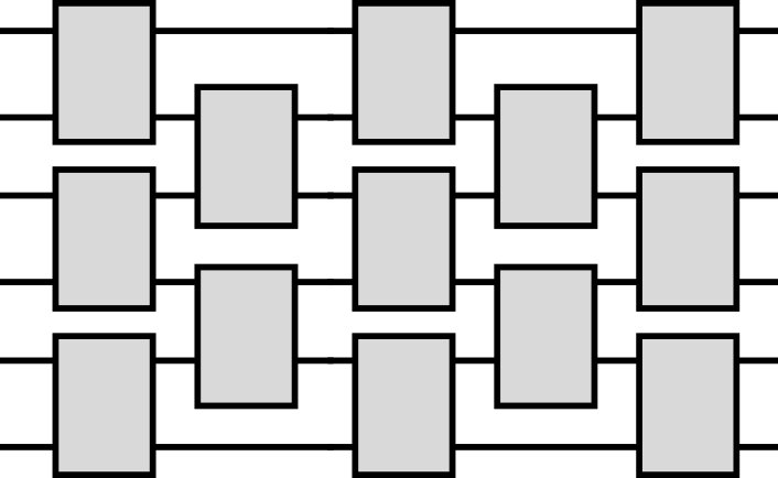
((a)) Brickwork circuit architecture. An example with 6 qubits and 5 layers.

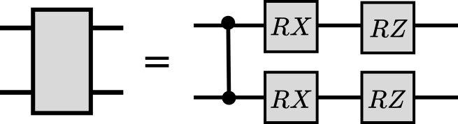
((b)) An individual block

Figure 5: Circuit structure used in numerical experiments.

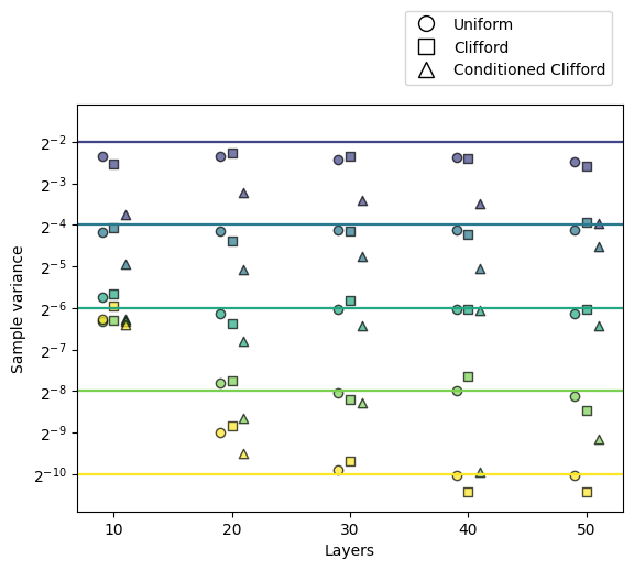
((a)) Sample variances of single-Pauli loss functions, averaged over all weight-two nearest-neighbor Pauli strings. Points denoted by $\bigcirc$ are obtained from the uniform sampling of angles, denoted by $\square$ from Clifford sampling. Points denoted by $\triangle$ correspond to statistic over Clifford points, conditioned on having at least one Pauli loss with non-zero value. The number of qubits ($n=2,4,6,8$ or $10$) at each data point is indicated by the color, and coincides with the exponent of the respective horizontal line.

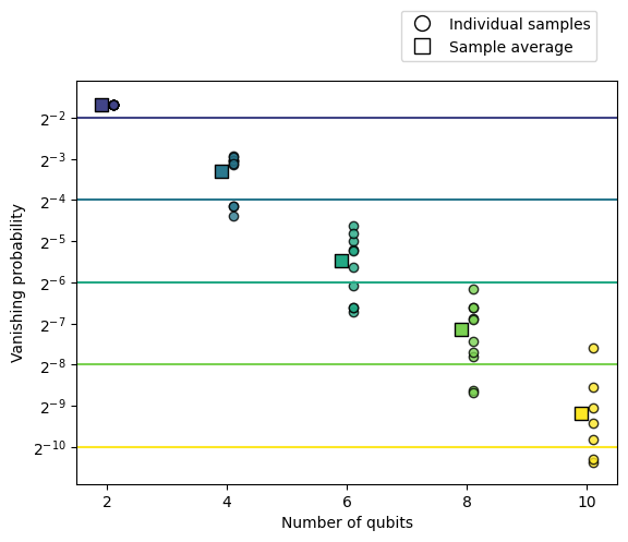
((b)) Vanishing probabilities of values and gradients of single-Pauli loss functions, averaged over all weight-two Pauli strings (independent of those defining the candidate exact local minimum). $\bigcirc$ show average vanishing probabilities for individual local minimums (10 points per each value of $n$), $\square$ show averages of all individual points at a given number of qubits.

Figure 6: Numerical results testing the existence of (a) approximate and (b) exact siloed local minima.

Here, we describe numerical experiments probing our theoretical predictions for the case of expressivity-induced BPs. Generally, numerically quantifying signatures of BPs is challenging, because resolving exponentially small variances requires exponential number of samples. Fortunately, the exponential decay with exponent $2^{-n}$ is expected to hold for small values of $n$ as well (see e.g. (12), which is valid for any $n$), and allows making quantitative comparisons even with a few-qubit circuits.

In our setup, the circuit has a standard brickwork architecture as depicted in Fig. 5(a), where each brick acts on two neighboring qubits and consists of a controlled $Z$ gate followed by an $R_{X}$ and $R_{Z}$ rotation on each qubit Fig. 5(b). When enough layers are present, the circuit furnishes a 2-design. Our experiments utilize circuits with different number of qubits and layers, but the general structure is shared by all instances. The initial state is always an all-zero computation basis state $\rho=(|0\rangle\langle 0|)^{\otimes n}$.

Further, we employ two different sets of observables. The first one, denoted by $\mathcal{P}_{2}^{NN}$, consists of all nearest-neighbor Pauli operators of weight two (e.g. $Z_{1}X_{2},Y_{3}X_{4}$) and contains $|\mathcal{P}_{2}^{NN}|=9(n-1)$ elements. The second one $\mathcal{P}_{2}$ includes all Pauli strings of weight two, not necessarily nearest-neighbor (e.g. $Z_{1}X_{5}$), and has $|\mathcal{P}_{2}|=9n(n-1)/2$ elements.

As a warm-up, we test that uniformly sampling parameters $\boldsymbol{\phi}$ yields the expected exponential decay of loss variance for deep enough circuits. To this end, we compute sample variance for each Pauli string from $\mathcal{P}_{2}^{NN}$ and report average variance in Fig. 6(a). Results are in good agreement with the expected variance scaling. We then repeat the same experiment, this time sampling parameters from the set of Clifford points $\boldsymbol{\phi_{\mathcal{C}}}$, as in (8), and verify that the resulting variances agree with $2^{-n}$ scaling as well. Details of the computational setup, such as the number of samples per observable, are given in App. C.

The next test we perform is non-trivial, and directly checks the validity of the second (independence) assumption of Thm. (2) in the current setup, which implies the existence of approximate LM as discussed in Sec. III.2. To probe if there are correlations between non-zero values of different Pauli observables, we take the data from the previous step, and only keep the Clifford points $\boldsymbol{\phi}_{c}$ which provide non-zero value to at least one of the Pauli observables from $\mathcal{P}_{2}^{NN}$. We collect the variance statistics over such Clifford points (filtered by having at least one Pauli string with non-vanishing expectation value), and report it in Fig. (6(a)). There are no signs of positive correlation between non-zero values of the observables, i.e. choosing a Clifford point $\boldsymbol{\phi}_{c}$, conditioned only on optimizing a single Pauli observable from $\mathcal{P}_{2}^{NN}$ but otherwise random, does not seem to bias other Pauli strings towards having non-zero values.

The second experiment provides a partial test for the existence of exact LM, as described in Sec. III.5, and proceeds as follows. We sample Clifford points from $\boldsymbol{\phi_{\mathcal{C}}}$ at random, and evaluate all weight two Pauli observables from $\mathcal{P}_{2}$, until we find a Pauli string $P_{i_{1}}$ with expectation value $-1$. We identify fixed angles $\boldsymbol{\theta}_{i_{1}}$ and null directions $\boldsymbol{\varphi}$ corresponding to this Clifford point. Then, keeping $\boldsymbol{\theta}_{i_{1}}$ fixed, we sample Clifford values of null directions $\boldsymbol{\varphi}$ until finding the next Pauli string $P_{i_{2}}$ with expectation value $-1$, and update the fixed $\boldsymbol{\theta}_{i_{1}i_{2}}$ and null directions $\boldsymbol{\varphi}$. We continue this process until no more Pauli strings can be added, obtaining a number of optimized Pauli stings $P_{I}=P_{i_{1}},P_{i_{2}},\dots$ and the candidate exact LM $(\boldsymbol{\theta}_{I},\boldsymbol{\varphi})$. In practice, we need to impose a threshold on the number of Clifford points to sample, before we consider that adding another Pauli observable is not possible. Details are specified in App. C.

Having a candidate exact LM, our goal is to check if the remaining terms, corresponding to Pauli strings from $\mathcal{P}_{2}$ not appearing in $P_{I}$, are exactly zero as a function of $\boldsymbol{\varphi}$, and so are their gradient (and Hessian) components. To confirm that a loss function $L(\boldsymbol{\phi})$ is exactly zero, we sample its values at several uniform points, and verify they are all zero up to a machine precision. For a moderate number of qubits that we work with, the expected variance (about $2^{-10}\approx 10^{-3}$ at worst for $n=10$) is orders of magnitude above machine precision, so we expect this test to be fairly robust.

A more difficult part is to verify that all gradient components are vanishing. While the number of gradient components scales only polynomially, for a few qubits the variance is not sufficiently small to suppress all of them. For instance, Ref. [14] estimated that on a linear topology, depth around $d=10n$ onsets a BP. The corresponding number of parameters (and hence the gradient components) is around $|\boldsymbol{\phi}|=10n^{2}$, and one needs to go significantly beyond $n=10$ qubits to make the variance scaling $2^{-n}$ dominant. Instead, we resort to a simpler test, checking the vanishing probability of each gradient component individually.

The final subtlety to our experiment arises from certain peculiarities of the Clifford VQAs at Clifford points. Namely, if two Pauli strings $P_{1},P_{2}$ have non-zero values at some Clifford point $\boldsymbol{\phi}_{c}$, so will their product. Indeed, $U(\boldsymbol{\phi}_{c})^{\dagger}P_{1}U(\boldsymbol{\phi}_{c})$ can only have a non-zero expectation value in $\rho=(|0\rangle\langle 0|)^{\otimes n}$ if it consists entirely of $I$ and $Z$ single-qubit Pauli operators, and the same holds for $P_{2}$. But then their product $U^{\dagger}(\boldsymbol{\phi}_{c})P_{1}P_{2}U(\boldsymbol{\phi}_{c})=U^{\dagger}(\boldsymbol{\phi}_{c})P_{1}U(\boldsymbol{\phi}_{c})U^{\dagger}(\boldsymbol{\phi}_{c})P_{2}U(\boldsymbol{\phi}_{c})$ again only contains $I$ and $Z$ factors, and has a non-vanishing value. Therefore, if a Clifford point optimizes Pauli operators $P_{1},P_{2},\dots$, it also renders the expectation value of any Pauli string generated from them non-zero. Because our Pauli stings come from a set of polynomial (and, in fact, quadratic) size $\mathcal{P}_{2}$, it is necessary to exclude any Pauli string that can be generated by $P_{I}$ from $\mathcal{P}_{2}$ to observe exponential decay of the variance.

With these limitations addressed, we report our numerical results in Fig. 6(b). Overall, while the mean vanishing probabilities do not precisely match the anticipated values, the overall decay with exponent around $2$ is clearly visible. We also note that the qualitative behavior of the process described in Sec. III.5 agrees well with numerics. In particular, every additional Pauli generator $P_{i_{k}}$ added while searching for exact minimum reduces the number of null direction approximately in half, and the total number of optimized Pauli generators $P_{I}$ is close to the theoretical value $\log_{2}|\boldsymbol{\phi}|$ for most trials.

V Discussion

In this work, we have argued that loss functions of Clifford VQAs subject to BPs are likely to contain exponentially many approximate siloed LM, which optimize for a single Pauli observable ignoring all others, as well as exact siloed LM, optimizing only $\mathcal{O}(\log n)$ independent Pauli observables. Apparently, there are many avenues to strengthen and generalize our results, but also many limitations to point out.

One may wonder whether good solutions are present in the landscape at all. Indeed, given that the LM of individual terms $L_{i}$ in the loss function are exponentially narrow, and that there is no a priori guarantee that LM of different terms overlap, the siloed LM may be the only solutions in some cases. In other cases, non-siloed LM may exist, but only in the shallow circuit regime. Apparently, making this kind of analysis quantitative requires to examine specifics of the variational ansatz, and we leave this interesting question for future work.

Let us note that our results are compatible with the overparameterization phenomenon in VQA [16, 11, 12], which suggests that loss landscapes with sufficiently many parameters have most LM exponentially close in value to the global minimum. The necessary number of parameters to achieve overparameterization is of the order of VQA’s dynamical Lie algebra dimension, which is exponentially large in a typical BP scenario. So, although by Thm. 1, the probability of any individual gradient or hessian component being non-zero is still exponentially small, the probability that some non-zero components exists can be of order one in the overparameterized regime.

The key technical limitation of our work is reliance on a specific type of VQAs. However, while the properties of Clifford VQAs were instrumental to obtain exact results with simple proofs, we expect that the qualitative conclusions may apply more broadly. Apparently, the most essential ingredient for our line of reasoning was the fact that individual Pauli observables have LM with large enough absolute loss values (of order one, as opposed to exponentially small). If a similar property is found in another VQA, we expect it to be accompanied by the siloed LM.

However, analyzing the loss landscapes of individual terms in general VQAs seems to be a challenging task. Examples include VQA with correlated parameters, non-Clifford gates, or based on non-standard dynamical Lie algebras [55, 56]. In all these cases, clarifying the structure of the loss landscape of individual observables may require a challenging and problem-specific analysis. It may happen, in principle, that such deformations of the Clifford VQA structure spare them from the siloed LM. However, it also seems possible that the resulting landscapes will generally lack any good solutions at all, similarly to the noise-induced BP landscapes. We leave this interesting question for future work.

Appendix A Trigonometric polynomials

A.1 Proof of Lemma 1

We call a single-variable function $F(\phi)$ a trigonometric polynomial of degree $2$ if it admits the following representation

$$F(\phi)=a+b\cos\phi+c\sin\phi+d\cos 2\phi+e\sin 2\phi\ .$$ (14)

Note that using identities $\cos 2\phi=2\cos^{2}\phi-1,\sin 2\phi=2\cos\phi\sin\phi$ this can be equivalently be rewritten as $F(\phi)=a^{\prime}+b^{\prime}\cos\phi+c^{\prime}\sin\phi+d^{\prime}\cos^{2}\phi+e^{\prime}\sin^{2}\phi+f^{\prime}\cos\phi\sin\phi$ with some coefficients $a^{\prime},\dots,f^{\prime}$.

The average of $F(\phi)$ over $\phi\in[0,2\pi]$ is simply $\mathbb{E}[F]=a$. In the single-variable case, Lemma 1 is then equivalent to the statement that $4a=F(0)+F(\pi/2)+F(\pi)+F(3\pi/2)$ and can be readily verified.

The multi-variable case is essentially the same. We call $F(\boldsymbol{\phi})$ a trigonometric polynomial of degree $2$ with respect to each variable, if Eq. (14) holds for every component of the parameter vector $\phi_{k}\in\boldsymbol{\phi}$ (the coefficients of the expansion can depend on the rest of components in $\boldsymbol{\phi}$, e.g. $F=\cos 2\phi_{1}\cos 2\phi_{2}$ is still of degree 2). The averaging over $\boldsymbol{\phi}$ is equivalent to sequential averaging over its components, and Lemma 1 follows.

A.2 Loss function

When a generator of the parameterized gate $e^{-iG\phi/2}$ squares to identity $G^{2}=\mathbb{I}$, the unitary of the quantum circuit satisfies $U(\phi)=\cos{\frac{\phi}{2}}U_{0}+\sin\frac{\phi}{2}U_{1}$ with $U_{0}=U(\phi=0),U_{1}=U(\phi=\pi)$. The loss function (1) then has the form

$$L(\phi)=\cos^{2}\frac{\phi}{2}\operatorname{Tr}[\rho\,\,U_{0}OU_{0}^{\dagger}]+\sin^{2}\frac{\phi}{2}\operatorname{Tr}[\rho\,\,U_{1}OU_{1}^{\dagger}]+\\ \cos\frac{\phi}{2}\sin\frac{\phi}{2}\operatorname{Tr}[\rho\,\,(U_{0}OU_{1}^{\dagger}+U_{1}OU_{0}^{\dagger})]\ .$$ (15)

Equivalently, it can be written as $L(\phi)=a+b\cos\phi+c\sin\phi$. Hence, $L(\phi)$ is a trigonometric polynomial of degree one, and $L^{2}(\phi)$ of degree two, and both satisfy the assumptions of Lemma 1.

A.3 Loss function average in Clifford VQA

Here we argue, that assuming $\mathbb{E}[L]=0$ in a Clifford VQA causes no loss of generality. While not necessary for our main argument, this fact simplifies the exposition and further clarifies the structure of loss function in Clifford VQA.

We will show, that loss function $L_{i}$ for any individual Pauli observable $P_{i}$ either (i) is constant $L_{i}(\boldsymbol{\phi})=\text{const}$ or (ii) has zero average $\mathbb{E}[L_{i}]=0$. The Pauli observables with constant loss functions can be simply ignored, while the rest have zero expectation value.

To show that $L_{i}$ is either constant or have zero average, it is convenient to transform the original circuit. All the constant Clifford gates can be commuted through the Pauli rotations to the end of the circuit, and then absorbed into a redefined observable $O^{\prime}$. Hence, the circuit can be written as $U^{\prime}(\boldsymbol{\phi})=\prod_{k}e^{-iP^{\prime}_{k}\phi_{k}/2}$ (generators $P^{\prime}_{k}$ are in general different from the generators of the original circuit $P_{k}$, because of the latter are transformed during the movement of the Clifford gates).

Now, there are two possibilities. The first is that all generators $P^{\prime}_{k}$ commute with the observable $O^{\prime}$, and therefore the corresponding loss function is trivially constant. The second case is when there exists some $P^{\prime}_{k}$ anti-commuting with $O^{\prime}$. Let $P^{\prime}_{r}$ be the first such gate in the Heisenberg picture, i.e.

$$L(\boldsymbol{\phi})=\operatorname{Tr}\left[\rho\,\,e^{iP^{\prime}_{1}\phi_{1}/2}\cdots e^{iP^{\prime}_{r}\phi_{r}/2}O^{\prime}e^{-iP^{\prime}_{r}\phi_{r}/2}\cdots e^{iP^{\prime}_{1}\phi_{1}/2}\right]\ .$$ (16)

Then,

$$e^{iP^{\prime}_{r}\phi_{r}/2}O^{\prime}e^{-iP^{\prime}_{r}\phi_{r}/2}=e^{iP^{\prime}_{r}\phi_{r}}O^{\prime}=\\ \cos\phi_{r}O^{\prime}+iP^{\prime}_{r}O^{\prime}\sin\phi_{r}$$ (17)

Therefore, the average of $L(\boldsymbol{\phi})$ with respect to $\phi_{r}$ vanishes, and so does the joint average with respect to all angles $\boldsymbol{\phi}$.

A.4 Fourier expansion

The full trigonometric polynomial of the loss function is in fact the same object as its Fourier expansion [57], that recently has been studied from a number of angles [58, 59, 60, 61, 62, 63, 64, 65, 50].

The full Fourier expansion can be organized in levels, where level $l$ only features terms that contain $l$ angles, e.g. $\cos\phi_{1}\cdots\cos\phi_{l}$. A general Fourier series for a VQA that has $m$ parameters can contain up to $3^{m}$ terms, for Clifford VQA with a single Pauli observable the upper bound is $2^{m}$ terms [65]. A typical VQA contains exponentially many terms in its Fourier expansion, but with the exponent less than two. For instance, for circuits with random non-local observables, there are $2^{-n}\left(\frac{3}{2}\right)^{m}$ terms on average.

Appendix B Exceptions

B.1 No null directions

((a))

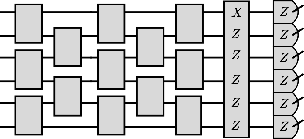
((b))

Figure 7: (a) A VQA with no null directions at critical points. (b) A VQA where the presence of BP depends on the state of a single gate.

A simple example of a VQA that does not admit null directions at the Clifford points is depicted in Fig. 7(a). It contains a single-qubit Pauli rotation on each qubit $U(\boldsymbol{\phi})=R_{X}(\phi_{1})\otimes\cdots\otimes R_{X}(\phi_{n})$, and the observable is $O=Z_{1}\cdots Z_{n}$. The loss function is simply $L=\prod_{k=1}^{n}\cos\phi_{k}$, and all local extrema correspond to $\phi_{k}=0,\pi$, where all $|\cos\phi_{k}|=1$ and hence $L=\pm 1$. Perturbing any of the angles shifts away from a critical point.

This example, however, appears to be rather contrived. For one, it features a specially chosen global observable. More importantly, the Fourier expansion of this loss function looks very atypical – it contains a single term at the largest level. Each term in the Fourier expansion corresponds to a Clifford point, where the value of the loss function equals $\pm 1$. The number of null directions at a Clifford point, corresponding to a term at level $l$, is simply $m-l$. It was demonstrated in Ref. [65] that the distribution of terms by level in a Fourier expansion typically shows a bell-type curve, centered around $m_{0}=m/2$ for non-local loss, and at $m_{0}\leq m/2$ for local loss functions. As argued in Sec. V we generically expect at least $m/2$ null directions, the same estimate that comes from the distribution of terms in the Fourier expansion. While we do not rule out the existence of interesting examples of VQA having most of the Fourier terms clustered at high levels, they are certainly not generic, and do not include e.g. QAOA or hardware-efficient circuits [65].

B.2 Barren plateau from a single gate

A VQA in Fig. 7(b) gives a simple yet contrived example, where switching a single gate can eliminate the BP. The first part of the circuit is assumed to be local and shallow, while the last gate is a global Pauli rotation with generator $P=X_{1}Z_{2}\cdots Z_{n}$. The observable $O=Z_{1}\dots Z_{n}$ is also non-local. When the angle of the global Pauli gate is zero, the VQA has a BP due to non-locality of the observable. However, choosing the angle $\phi=\frac{\pi}{2}$, so that the Pauli rotation gate is $e^{-iP\frac{\pi}{4}}$, effectively removes the non-locality of the observable since $e^{iP\frac{\pi}{4}}Oe^{-iP\frac{\pi}{4}}=e^{iP\frac{\pi}{2}}O=iPO=Y_{1}$. Hence, the resulting VQA is not expected to have a BP.

B.3 Variance of a loss function with a random observable

Here we prove relation (12). First, note that inequality $\mathbb{V}[L_{P}]=\mathbb{E}[L_{P}^{2}]-\mathbb{E}[L_{P}]^{2}\leq\mathbb{E}[L_{P}^{2}]$ holds for any random variable $L_{P}$. Next, according to (8), the expectation value $\mathbb{E}[L_{P}^{2}]$ can be represented as a sum over Clifford points of the form

$$L_{P}^{2}(\boldsymbol{\phi}_{c})=\langle 0|U(\boldsymbol{\phi}_{c})^{\dagger}PU(\boldsymbol{\phi}_{c})|0\rangle^{2}\ .$$ (18)

The average value over $P$ for any choice of $\boldsymbol{\phi}_{c}$ is simply equal to

$$\mathbb{E}_{P}[L_{P}^{2}(\boldsymbol{\phi}_{c})]=\mathbb{E}_{P}\left[\langle 0|U(\boldsymbol{\phi}_{c})^{\dagger}PU(\boldsymbol{\phi}_{c})|0\rangle^{2}\right]=\\ \mathbb{E}_{P}\left[\langle 0|P|0\rangle^{2}\right]=2^{-n}\ ,$$ (19)

which is just a probability that a random Pauli operator has a non-vanishing expectation value in the all-zero state $\rho=(|0\rangle\langle 0|)^{\otimes n}$. Relation (12) thus follows.

Appendix C Details of numerical experiments

Both experiments reported in Fig. 6 use circuit layouts specified in Fig. 5 with number of qubits varying from $n=2$ to $n=10$ and number of layers between $10$ and $50$. All circuits simulated in Fig. 6(b) have 50 layers.

To gather data for Fig. 6(a), for each pair (number of qubits, number of layers) and for each observable from $\mathcal{P}_{2}^{NN}$ we sample 50 values of $\boldsymbol{\phi}$ from a uniform distribution, and 50 Clifford values. Note that the for 10-qubit circuits at 30 and 50 layers the conditioned Clifford marker $\triangle$ is absent, because no Clifford points with more than a single non-zero Pauli appeared during sampling.

The data for Fig. 6(b) was obtained along the lines described in the main section Sec. IV. We are not aware of any efficient procedure that, for a given circuit and Pauli observable, finds a Clifford point where this observable has non-zero expectation. Thus, we resort to extensive sampling over Clifford points and trying many observables in parallel. For this reason, in this experiment, we choose a larger set of non-nearest neighbor Pauli strings $\mathcal{P}_{2}$.

For each number of qubits we perform 10 trials, each producing a potential exact LM, and compute the statistics over remaining loss function terms at these points. Each individual trial is depicted by $\bigcirc$ in Fig. 6(b). The average value over all trials for a given number of qubits is depicted by $\square$.

While looking for the next Pauli operator to add, we compute values of all independent Pauli operators from $\mathcal{P}_{2}$ at

$$\left\lfloor 30\frac{2^{n}}{|\mathcal{P}_{2}|}\right\rfloor\approx 3\frac{2^{n}}{n^{2}}$$ (20)

random Clifford points. We scale the number of sampled points exponentially, to keep the probability of finding non-zero expectation values high enough. If no Pauli operators with non-zero expectation values were found among the sampled points, we stop the search for additional Pauli operators. In two cases for $n=10$ qubit circuit this procedure did not produce even a single Pauli operator, and the number of individual samples depicted at Fig. 6(b) for $n=10$ is correspondingly reduced.

This procedure ends by proposing an exact LM, optimizing several Pauli terms $P_{I}$ and induces a split of the parameter space $(\boldsymbol{\theta}_{I},\boldsymbol{\varphi})$. We then test if the loss functions, corresponding to Pauli terms, remaining in $\mathcal{P}_{2}$ and independent of $P_{I}$, are identically zero as functions of $\boldsymbol{\varphi}$. We also test that their gradients with respect to $\boldsymbol{\theta}_{I}$ are identically vanishing as well. We chose not to study Hessian entries, but expect largely similar results in this case.

As discussed in Sec. IV, the number of gradient components for deep enough circuits is substantial. Hence, we limit the number of gradient components (chosen at random for each trial) evaluated for each observable from $\mathcal{P}_{2}$ by the same value featuring in Eq. 20. We consider each loss function or gradient component corresponding to an observable from $\mathcal{P}_{2}$ to be exactly vanishing, if the variance estimated over 10 uniformly sampled points is zero within the machine precision.

The code producing the numerical results reported here is mostly written using PennyLane library [66], and is available at [67].

References

- [1] M. Cerezo, Andrew Arrasmith, Ryan Babbush, Simon C. Benjamin, Suguru Endo, Keisuke Fujii, Jarrod R. McClean, Kosuke Mitarai, Xiao Yuan, Lukasz Cincio, and Patrick J. Coles. “Variational quantum algorithms”. Nature Reviews Physics 2021 3:9 3, 625–644 (2021). arXiv:2012.09265.
- [2] Jacob Biamonte, Peter Wittek, Nicola Pancotti, Patrick Rebentrost, Nathan Wiebe, and Seth Lloyd. “Quantum machine learning”. Nature 549, 195–202 (2017). arXiv:1611.09347.
- [3] Maria Schuld, Ilya Sinayskiy, and Francesco Petruccione. “An introduction to quantum machine learning”. Contemporary Physics 56, 172–185 (2015). arXiv:1409.3097v1.
- [4] John Preskill. “Quantum computing in the NISQ era and beyond”. Quantum 2, 1–20 (2018). arXiv:1801.00862.
- [5] Kishor Bharti, Alba Cervera-Lierta, Thi Ha Kyaw, Tobias Haug, Sumner Alperin-Lea, Abhinav Anand, Matthias Degroote, Hermanni Heimonen, Jakob S. Kottmann, Tim Menke, Wai-Keong Mok, Sukin Sim, Leong-Chuan Kwek, and Alán Aspuru-Guzik. “Noisy intermediate-scale quantum (NISQ) algorithms”. Reviews of Modern Physics94 (2021). arXiv:2101.08448v2.
- [6] A. K. Fedorov, N. Gisin, S. M. Beloussov, and A. I. Lvovsky. “Quantum computing at the quantum advantage threshold: a down-to-business review” (2022). arXiv:2203.17181.
- [7] Supanut Thanasilp, Samson Wang, Nhat A. Nghiem, Patrick J. Coles, and M. Cerezo. “Subtleties in the trainability of quantum machine learning models”. Quantum Machine Intelligence5 (2021). arXiv:2110.14753.
- [8] Manuel S. Rudolph, Sacha Lerch, Supanut Thanasilp, Oriel Kiss, Sofia Vallecorsa, Michele Grossi, and Zoë Holmes. “Trainability barriers and opportunities in quantum generative modeling” (2023). arXiv:2305.02881.
- [9] Ian Goodfellow, Yoshua Bengio, and Aaron Courville. “Deep learning”. MIT Press. (2016). url: http://www.deeplearningbook.org.
- [10] Lennart Bittel and Martin Kliesch. “Training Variational Quantum Algorithms Is NP-Hard”. Physical Review Letters 127, 120502 (2021). arXiv:2101.07267.
- [11] Eric R. Anschuetz. “Critical Points in Quantum Generative Models” (2021). arXiv:2109.06957.
- [12] Eric R. Anschuetz and Bobak T. Kiani. “Quantum variational algorithms are swamped with traps”. Nature Communications 13, 7760 (2022). arXiv:2205.05786.
- [13] Xuchen You and Xiaodi Wu. “Exponentially Many Local Minima in Quantum Neural Networks”. Proceedings of Machine Learning Research 139, 12144–12155 (2021). arXiv:2110.02479.
- [14] Jarrod R. McClean, Sergio Boixo, Vadim N. Smelyanskiy, Ryan Babbush, and Hartmut Neven. “Barren plateaus in quantum neural network training landscapes”. Nature Communications 9, 1–7 (2018). arXiv:1803.11173.
- [15] Martin Larocca, Supanut Thanasilp, Samson Wang, Kunal Sharma, Jacob Biamonte, Patrick J. Coles, Lukasz Cincio, Jarrod R. McClean, Zoë Holmes, and M. Cerezo. “A Review of Barren Plateaus in Variational Quantum Computing” (2024). arXiv:2405.00781.
- [16] Martin Larocca, Nathan Ju, Diego García-Martín, Patrick J. Coles, and M. Cerezo. “Theory of overparametrization in quantum neural networks” (2021). arXiv:2109.11676.
- [17] Ernesto Campos, Aly Nasrallah, and Jacob Biamonte. “Abrupt transitions in variational quantum circuit training”. Physical Review A103 (2021). arXiv:2010.09720.
- [18] E. Campos, D. Rabinovich, V. Akshay, and J. Biamonte. “Training Saturation in Layerwise Quantum Approximate Optimisation”. Physical Review A104 (2021). arXiv:2106.13814v1.
- [19] Bobak Toussi Kiani, Seth Lloyd, and Reevu Maity. “Learning Unitaries by Gradient Descent” (2020). arXiv:2001.11897.
- [20] Nikita A. Nemkov, Evgeniy O. Kiktenko, Ilia A. Luchnikov, and Aleksey K. Fedorov. “Efficient variational synthesis of quantum circuits with coherent multi-start optimization”. Quantum 7, 993 (2023). arXiv:2205.01121.
- [21] Edward Farhi, Jeffrey Goldstone, and Sam Gutmann. “A Quantum Approximate Optimization Algorithm” (2014). arXiv:1411.4028.
- [22] Abhinav Kandala, Antonio Mezzacapo, Kristan Temme, Maika Takita, Markus Brink, Jerry M. Chow, and Jay M. Gambetta. “Hardware-efficient Variational Quantum Eigensolver for Small Molecules and Quantum Magnets”. Nature 549, 242–246 (2017). arXiv:1704.05018.
- [23] Jonathan Romero, Ryan Babbush, Jarrod R. McClean, Cornelius Hempel, Peter J. Love, and Alán Aspuru-Guzik. “Strategies for quantum computing molecular energies using the unitary coupled cluster ansatz”. Quantum Science and Technology 4, 014008 (2018). arXiv:1701.02691.
- [24] Arthur Pesah, M. Cerezo, Samson Wang, Tyler Volkoff, Andrew T. Sornborger, and Patrick J. Coles. “Absence of Barren Plateaus in Quantum Convolutional Neural Networks”. Physical Review X 11, 041011 (2021). arXiv:2011.02966.
- [25] Martin Larocca, Piotr Czarnik, Kunal Sharma, Gopikrishnan Muraleedharan, Patrick J. Coles, and M. Cerezo. “Diagnosing Barren Plateaus with Tools from Quantum Optimal Control”. Quantum 6, 824 (2022). arXiv:2105.14377v3.
- [26] Martín Larocca, Frédéric Sauvage, Faris M. Sbahi, Guillaume Verdon, Patrick J. Coles, and M. Cerezo. “Group-Invariant Quantum Machine Learning”. PRX Quantum 3, 030341 (2022). arXiv:2205.02261.
- [27] Johannes Jakob Meyer, Marian Mularski, Elies Gil-Fuster, Antonio Anna Mele, Francesco Arzani, Alissa Wilms, and Jens Eisert. “Exploiting symmetry in variational quantum machine learning” (2022). arXiv:2205.06217.
- [28] M. Cerezo, Martin Larocca, Diego García-Martín, N. L. Diaz, Paolo Braccia, Enrico Fontana, Manuel S. Rudolph, Pablo Bermejo, Aroosa Ijaz, Supanut Thanasilp, Eric R. Anschuetz, and Zoë Holmes. “Does provable absence of barren plateaus imply classical simulability? Or, why we need to rethink variational quantum computing” (2023). arXiv:2312.09121.
- [29] Andrea Skolik, Jarrod R. McClean, Masoud Mohseni, Patrick van der Smagt, and Martin Leib. “Layerwise learning for quantum neural networks”. Quantum Machine Intelligence3 (2020). arXiv:2006.14904v1.
- [30] Edward Grant, Leonard Wossnig, Mateusz Ostaszewski, and Marcello Benedetti. “An initialization strategy for addressing barren plateaus in parametrized quantum circuits”. Quantum 3, 214 (2019). arXiv:1903.05076v3.
- [31] Kaining Zhang, Liu Liu, Min-Hsiu Hsieh, and Dacheng Tao. “Escaping from the Barren Plateau via Gaussian Initializations in Deep Variational Quantum Circuits”. Advances in Neural Information Processing Systems35 (2022). arXiv:2203.09376.
- [32] Yabo Wang, Bo Qi, Chris Ferrie, and Daoyi Dong. “Trainability Enhancement of Parameterized Quantum Circuits via Reduced-Domain Parameter Initialization” (2023). arXiv:2302.06858.
- [33] Manuel S. Rudolph, Jacob Miller, Danial Motlagh, Jing Chen, Atithi Acharya, and Alejandro Perdomo-Ortiz. “Synergy Between Quantum Circuits and Tensor Networks: Short-cutting the Race to Practical Quantum Advantage” (2022). arXiv:2208.13673.
- [34] Gokul Subramanian Ravi, Pranav Gokhale, Yi Ding, William M. Kirby, Kaitlin N. Smith, Jonathan M. Baker, Peter J. Love, Henry Hoffmann, Kenneth R. Brown, and Frederic T. Chong. “CAFQA: Clifford Ansatz For Quantum Accuracy” (2022). arXiv:2202.12924.
- [35] Andrew Arrasmith, Zoë Holmes, M. Cerezo, and Patrick J. Coles. “Equivalence of quantum barren plateaus to cost concentration and narrow gorges”. Quantum Science and Technology 7, 045015 (2022). arXiv:2104.05868v2.
- [36] Qiang Miao and Thomas Barthel. “Equivalence of cost concentration and gradient vanishing for quantum circuits: an elementary proof in the Riemannian formulation” (2024). arXiv:2402.07883.
- [37] Zoë Holmes, Kunal Sharma, M. Cerezo, and Patrick J. Coles. “Connecting Ansatz Expressibility to Gradient Magnitudes and Barren Plateaus”. PRX Quantum 3, 010313 (2022). arXiv:2101.02138v2.
- [38] Christoph Dankert, Richard Cleve, Joseph Emerson, and Etera Livine. “Exact and approximate unitary 2-designs and their application to fidelity estimation”. Physical Review A 80, 012304 (2009). arXiv:0606161.
- [39] Aram W. Harrow and Saeed Mehraban. “Approximate Unitary t-Designs by Short Random Quantum Circuits Using Nearest-Neighbor and Long-Range Gates”. Communications in Mathematical Physics 401, 1531–1626 (2023). arXiv:1809.06957.
- [40] M. Cerezo, Akira Sone, Tyler Volkoff, Lukasz Cincio, and Patrick J. Coles. “Cost function dependent barren plateaus in shallow parametrized quantum circuits”. Nature Communications 2021 12:1 12, 1–12 (2021). arXiv:2001.00550.
- [41] A V Uvarov and J D Biamonte. “On barren plateaus and cost function locality in variational quantum algorithms”. Journal of Physics A: Mathematical and Theoretical 54, 245301 (2021). arXiv:2011.10530.
- [42] Sumeet Khatri, Ryan LaRose, Alexander Poremba, Lukasz Cincio, Andrew T. Sornborger, and Patrick J. Coles. “Quantum-assisted quantum compiling”. Quantum 3, 140 (2019). arXiv:1807.00800v5.
- [43] Tyson Jones and Simon C Benjamin. “Robust quantum compilation and circuit optimisation via energy minimisation”. Quantum 6, 628 (2022). arXiv:1811.03147v5.
- [44] Jonathan Romero, Jonathan P. Olson, and Alan Aspuru-Guzik. “Quantum autoencoders for efficient compression of quantum data”. Quantum Science and Technology 2, 045001 (2017). arXiv:1612.02806v2.
- [45] Carlos Ortiz Marrero, Mária Kieferová, and Nathan Wiebe. “Entanglement-Induced Barren Plateaus”. PRX Quantum 2, 040316 (2021). arXiv:2010.15968.
- [46] Kunal Sharma, M. Cerezo, Lukasz Cincio, and Patrick J. Coles. “Trainability of Dissipative Perceptron-Based Quantum Neural Networks”. Physical Review Letters 128, 180505 (2022). arXiv:2005.12458.
- [47] Mariia D. Sapova and Aleksey K. Fedorov. “Variational quantum eigensolver techniques for simulating carbon monoxide oxidation”. Communications Physics 5, 199 (2022).
- [48] Samson Wang, Enrico Fontana, M. Cerezo, Kunal Sharma, Akira Sone, Lukasz Cincio, and Patrick J. Coles. “Noise-induced barren plateaus in variational quantum algorithms”. Nature Communications 12, 6961 (2021). arXiv:2007.14384.
- [49] Daniel Stilck França and Raul García-Patrón. “Limitations of optimization algorithms on noisy quantum devices”. Nature Physics 17, 1221–1227 (2021). arXiv:2009.05532v1.
- [50] Enrico Fontana, Manuel S Rudolph, Ross Duncan, Ivan Rungger, and Cristina Cîrstoiu. “Classical simulations of noisy variational quantum circuits” (2023). arXiv:2306.05400.
- [51] Phattharaporn Singkanipa and Daniel A Lidar. “Beyond unital noise in variational quantum algorithms: noise-induced barren plateaus and fixed points” (2024). arXiv:2402.08721.
- [52] Kosuke Mitarai, Makoto Negoro, Masahiro Kitagawa, and Keisuke Fujii. “Quantum Circuit Learning”. Physical Review A98 (2018). arXiv:1803.00745.
- [53] Maria Schuld, Ville Bergholm, Christian Gogolin, Josh Izaac, and Nathan Killoran. “Evaluating analytic gradients on quantum hardware”. Physical Review A99 (2018). arXiv:1811.11184v1.
- [54] Naman Agarwal, Zeyuan Allen-Zhu, Brian Bullins, Elad Hazan, and Tengyu Ma. “Finding approximate local minima faster than gradient descent”. In Proceedings of the 49th Annual ACM SIGACT Symposium on Theory of Computing. Volume Part F1284, pages 1195–1199. New York, NY, USA (2017). ACM. arXiv:1611.01146.
- [55] Michael Ragone, Bojko N. Bakalov, Frédéric Sauvage, Alexander F. Kemper, Carlos Ortiz Marrero, Martin Larocca, and M. Cerezo. “A Unified Theory of Barren Plateaus for Deep Parametrized Quantum Circuits” (2023). arXiv:2309.09342.
- [56] Enrico Fontana, Dylan Herman, Shouvanik Chakrabarti, Niraj Kumar, Romina Yalovetzky, Jamie Heredge, Shree Hari Sureshbabu, and Marco Pistoia. “The Adjoint Is All You Need: Characterizing Barren Plateaus in Quantum Ans"atze” (2023). arXiv:2309.07902.
- [57] Maria Schuld, Ryan Sweke, and Johannes Jakob Meyer. “The effect of data encoding on the expressive power of variational quantum machine learning models”. Physical Review A103 (2020). arXiv:2008.08605v2.
- [58] Francisco Javier Gil Vidal and Dirk Oliver Theis. “Input Redundancy for Parameterized Quantum Circuits”. Frontiers in Physics 8, 297 (2020). arXiv:1901.11434.
- [59] Parfait Atchade-Adelomou and Kent Larson. “Fourier series weight in quantum machine learning” (2023). arXiv:2302.00105.
- [60] Berta Casas and Alba Cervera-Lierta. “Multi-dimensional Fourier series with quantum circuits” (2023). arXiv:2302.03389.
- [61] Franz J. Schreiber, Jens Eisert, and Johannes Jakob Meyer. “Classical surrogates for quantum learning models” (2022). arXiv:2206.11740.
- [62] Jonas Landman, Slimane Thabet, Constantin Dalyac, Hela Mhiri, and Elham Kashefi. “Classically Approximating Variational Quantum Machine Learning with Random Fourier Features” (2023).
- [63] Enrico Fontana, Ivan Rungger, Ross Duncan, and Cristina Cˆırstoiu Cˆırstoiu. “Efficient recovery of variational quantum algorithms landscapes using classical signal processing” (2022). arXiv:2208.05958.
- [64] Enrico Fontana, Ivan Rungger, Ross Duncan, and Cristina Cˆırstoiu Cˆırstoiu. “Spectral analysis for noise diagnostics and filter-based digital error mitigation” (2022). arXiv:2206.08811.
- [65] Nikita A. Nemkov, Evgeniy O. Kiktenko, and Aleksey K. Fedorov. “Fourier expansion in variational quantum algorithms”. Physical Review A 108, 032406 (2023). arXiv:2304.03787v2.
- [66] Ville Bergholm, Josh Izaac, Maria Schuld, Christian Gogolin, Shahnawaz Ahmed, Vishnu Ajith, M. Sohaib Alam, Guillermo Alonso-Linaje, B. AkashNarayanan, Ali Asadi, Juan Miguel Arrazola, Utkarsh Azad, Sam Banning, Carsten Blank, Thomas R Bromley, Benjamin A. Cordier, Jack Ceroni, Alain Delgado, Olivia Di Matteo, Amintor Dusko, Tanya Garg, Diego Guala, Anthony Hayes, Ryan Hill, Aroosa Ijaz, Theodor Isacsson, David Ittah, Soran Jahangiri, Prateek Jain, Edward Jiang, Ankit Khandelwal, Korbinian Kottmann, Robert A. Lang, Christina Lee, Thomas Loke, Angus Lowe, Keri McKiernan, Johannes Jakob Meyer, J. A. Montañez-Barrera, Romain Moyard, Zeyue Niu, Lee James O’Riordan, Steven Oud, Ashish Panigrahi, Chae-Yeun Park, Daniel Polatajko, Nicolás Quesada, Chase Roberts, Nahum Sá, Isidor Schoch, Borun Shi, Shuli Shu, Sukin Sim, Arshpreet Singh, Ingrid Strandberg, Jay Soni, Antal Száva, Slimane Thabet, Rodrigo A. Vargas-Hernández, Trevor Vincent, Nicola Vitucci, Maurice Weber, David Wierichs, Roeland Wiersema, Moritz Willmann, Vincent Wong, Shaoming Zhang, and Nathan Killoran. “PennyLane: Automatic differentiation of hybrid quantum-classical computations” (2018). arXiv:1811.04968.
- [67] N. Nemkov, E. Kiktenko, and A. Fedorov (2024). url: https://github.com/idnm/barren_traps.