First detection of CO isotopologues in a high-redshift main-sequence galaxy: evidence of a top-heavy stellar initial mass function

Abstract

Recent observations and theories have presented a strong challenge to the universality of the stellar initial mass function (IMF) in extreme environments. A notable example has been found for starburst conditions, where evidence favours a top-heavy IMF, i.e. there is a bias toward massive stars compared to the IMF that is responsible for the stellar mass function and elemental abundances observed in the Milky Way. Local starburst galaxies have star-formation rates similar to those in high-redshift main-sequence galaxies, which appear to dominate the stellar mass budget at early epochs. However, the IMF of high-redshift main-sequence galaxies is yet to be probed. Since ¹³CO and C¹⁸O isotopologues are sensitive to the IMF, we have observed these lines towards four strongly-lensed high-redshift main-sequence galaxies using the Atacama Large Millimeter/sub-millimeter Array. Of our four targets, SDSS J0901+1814, at $z\approx 2.26$, is seen clearly in ¹³CO and C¹⁸O, the first detection of CO isotopologues in the high-redshift main-sequence galaxy population. The observed ¹³C/¹⁸O ratio, $2.4\pm 0.8$, is significantly lower than that of local main-sequence galaxies. We estimate the isotope ratio, oxygen abundance and stellar mass using a series of chemical evolution models with varying star-formation histories and IMFs. All models favour an IMF that is more top-heavy than that of the Milky Way. Thus, as with starburst galaxies, main-sequence galaxies in the high-redshift Universe have a greater fraction of massive stars than a Milky-Way IMF would imply.

1 Introduction

When interpreting observations of starlight, infrared (IR) or radio continuum emission from galaxies – all typically dominated by energy from massive stars – the choice of the stellar initial mass function (IMF) is one of the most important assumptions we make. This is true whether one is looking at individual galaxies, or averaging over cosmological volumes (Kennicutt, 1998a; Madau & Dickinson, 2014). The choice of IMF has profound implications for the determination of star-formation rates (SFRs) and stellar masses, for example, both of which are used to define the so-called ‘main sequence’ of galaxies. The IMF can thus play a fundamental role in cosmological simulations of structure formation (Baugh et al., 2005), and in the interpretation of galaxy evolution across cosmic time (Daddi et al., 2007).

The IMF is usually assumed to be a universal and invariant function, based on observations in the Galaxy and the Magellanic Clouds (Kroupa, 2001; Bastian et al., 2010). Its universality can be understood in terms of the initial conditions for star formation, which occur in dense region deep inside molecular clouds and is well shielded from ultraviolet radiation and where supersonic turbulence is fully dissipated, so thermodynamically similar (Elmegreen et al., 2008). Cosmic rays (CRs) seem to be the only form of feedback that can strongly perturb the otherwise well-shielded initial conditions of star formation. Once a CR energy density background of $\sim$$10^{2}\times$ Galactic average has been reached (the Galactic average CR energy density is around 0.5–1.4 eV cm^-3; Yoast-Hull et al., 2016; Papadopoulos et al., 2011), as expected in starburst environments, the IMF may then be quite different from that of ordinary star-forming disks (Papadopoulos et al., 2011).

An increasing body of evidence points to a non-universal IMF, supported by observations of stellar properties in external galaxies (Rieke et al., 1993; Lee et al., 2009; Gunawardhana et al., 2011; Yan et al., 2020; Mucciarelli et al., 2021), CO isotope abundances in the interstellar medium (ISM; Romano et al., 2017; Zhang et al., 2018), and star counting in both the Milky Way and the Large Magellanic Cloud (Geha et al., 2013; Li et al., 2023; Schneider et al., 2018). It has been proposed that a non-universal IMF can account for the properties of galaxies under different physical conditions and at different evolutionary stages (Matteucci & Brocato, 1990; Yan et al., 2017; Jeřábková et al., 2018; Hopkins, 2018; Smith, 2020).

In dust-obscured, gas-rich star-forming galaxies there is no hope of following the classical method of probing their IMF directly, based on an assessment of the stellar light via optical/near-IR observations. However, sub-millimeter/millimeter (sub-mm/mm) wavelengths are largely unobscured by dust and provide an alternative probe of the IMF, opening a window to measure the isotopic abundances of particular elements in these systems. The isotopes of carbon, nitrogen and oxygen (see Romano, 2022, for a recent review) are particularly suitable for this purpose, since they are produced through different stellar nucleosynthesis processes in stars of different masses, and are thus released to the ISM on different timescales (Kobayashi et al., 2011; Romano et al., 2017; Zhang et al., 2018). For instance, ¹⁸O is produced predominantly by massive stars ($\geq 8$ ${\rm M}_{\odot}$) purely through secondary channels, while ¹³C is produced mainly by low- and intermediate-mass stars (LIMS, $<8$ ${\rm M}_{\odot}$), through primary plus secondary element channels (e.g., Portinari et al., 1998; Marigo, 2001; Romano et al., 2017).

These isotopes are ejected into the ISM via stellar winds (Romano, 2022), where they form molecules in the same way as their major isotopes, with similar astrochemical properties. Emission from ¹³CO and C¹⁸O transitions (isotopologues of ¹²C¹⁶O) can therefore be used to trace the ¹³C and ¹⁸O abundances produced by ancestral generations of stars. Abundance ratios of ¹³CO/C¹⁸O have been found to anti-correlate with the IR luminosity of large molecular gas reservoirs in local galaxies (Jiménez-Donaire et al., 2017; Zhang et al., 2018). The line ratio is found to be roughly unity in ultraluminous IR galaxies (ULIRGs) (Henkel et al., 2014; Sliwa et al., 2017; Brown & Wilson, 2019), in contrast to values ranging from 7 to 10 in the disk of the Milky Way and in local disk galaxies (Giannetti et al., 2014; Jiménez-Donaire et al., 2017). This can be and has been interpreted as an indication of a higher fraction of massive stars (i.e. a top-heavy IMF) in high-SFR galaxies.

Strengthening the correlation between IR luminosity ($L_{\rm IR}$) and the ¹³CO/C¹⁸O ratio found in local galaxies, low ¹³CO/C¹⁸O ratios have been found in strongly lensed starbursts at $z\sim 2$–3 (Danielson et al., 2013; Yang et al., 2023), which can be well reproduced in galactic chemical evolution (GCE) models with a top-heavy IMF (Zhang et al., 2018).

However, it is unclear whether high-redshift main-sequence galaxies – thought to contribute the majority of the cosmic SFR (Daddi et al., 2007; Madau & Dickinson, 2014) – still hold to the IMF adopted in most current work (e.g., Huang et al., 2023). In fact, these galaxies are known to have 1–2 orders of magnitude higher SFRs (Schreiber et al., 2015) and smaller sizes (and, therefore, higher SFR surface densities; Conselice, 2014), compared to those of local main-sequence galaxies with the same stellar masses. If these high-redshift main-sequence galaxies were in the local Universe, they would be classified as starbursts (Schreiber et al., 2015), raising the possibility that their star formation also proceeds with a top-heavy IMF.

As with their dust-enshrouded starburst brethren, it is difficult to examine the intrinsic stellar light – the ultraviolet/optical spectral energy distribution (SED) – of high-redshift main-sequence galaxies, because they contain high fractions of gas and dust (van der Giessen et al., 2022). This prevents the use of classical methods to derive their IMFs. However, recent Atacama Large Millimeter/sub-millimeter Array (ALMA) observations have detected CO emission from a few strongly-lensed, high-redshift main-sequence galaxies (e.g. Dessauges-Zavadsky et al., 2015, 2017; Sharon et al., 2019), which may allow the application of the ¹³C/¹⁸O diagnostic, despite the weak emission expected from these isotopologues.

Isotopic abundances are sensitive to the IMF, to the star-formation history (SFH), and to stellar nucleosynthesis, thus interpreting them requires sophisticated GCE modelling (Matteucci, 2001). As with previous work on starburst galaxies (Romano et al., 2017; Zhang et al., 2018), we use literature estimates of the stellar mass and metallicity ([O/H]) of the systems to constrain our GCE models. For this work, we use a modified version of the open-source GCE code, NuPyCEE (Côté et al., 2017; Ritter et al., 2018), to simulate the evolution of the galaxies.

This paper is organised as follows: in Section 2, we describe our observations, data reduction, and the ancillary data adopted in this work. Section 3 presents the observational results. In Section 4, we describe the assumptions and settings in the GCE model. Section 5 presents a comparison of the observational and modelling results. Section 6 discusses the possible IMF bias from SFH and spatial variation and the impact on the history of cosmic star formation. Throughout this paper, we use the Planck Collaboration et al. (2016) cosmology, with $\Omega_{\rm m}$ = 0.315, $\Omega_{\Lambda}$ = 0.685, $\Omega_{\rm b}$ = 0.0490, $h$ = 0.6731, $\sigma_{8}$ = 0.829 and $n_{\rm S}$ = 0.9655.

2 Observations and data reduction

2.1 ALMA observations

We have gathered a sample of four strongly lensed star-forming galaxies from the literature. Their peak flux density in a CO line is at least 10 mJy (cf. Table 1). Their range of redshifts spans $z=1.5$–3.6, which corresponds to roughly the epoch of maximal cosmic SFR density (e.g. Madau & Dickinson, 2014).

The intrinsic (i.e. corrected for lensing) SFRs and stellar masses of these galaxies are in the range 25–600 ${\rm M}_{\odot}\,{\rm yr}^{-1}$ and 5–$300\times 10^{9}$ ${\rm M}_{\odot}$, respectively (Dessauges-Zavadsky et al., 2017, 2015; Sharon et al., 2019). The SFR has been estimated from both the H$\alpha$ and from the total IR luminosity (Sharon et al., 2019); we adopt the latter because the SFR estimated from total IR luminosity is not affected by the dust obscuration in contrast to H$\alpha$. For the other three galaxies in our sample, the SFRs were determined from the best SED fits to the combination of the ultraviolet and IR luminosities. Fig. 1 presents all targets superimposed on the corresponding three main-sequence scaling relations, for $z=1.58$ (two target galaxies), 2.26 and 3.63; different colors refer to the different redshifts (see e.g. Schreiber et al., 2015). Our four targets are all located in or under their corresponding main sequence. The oxygen abundance of SDSS J0901+1814 is derived from the [N ii] and H$\alpha$ emission lines (Sharon et al., 2019; Pettini & Pagel, 2004), while for MACS J0032-arc it is estimated via the mass-metallicity relation (Dessauges-Zavadsky et al., 2017; Pettini & Pagel, 2004).

We observed the ¹³CO and C¹⁸O transitions towards our target galaxies using ALMA (programme 2018.1.00588.S: P.I. Zhi-Yu Zhang). The full 12-m array was employed, with 43–52 antennas. MACS J0032-arc, A68-CO and A68-LHS115 were observed in band 4; SDSS J0901+1814 was observed in band 3. Before and after each 10-min interval spent on the targets, we switched to a calibrator to track the complex gain fluctuations. For each spectral window (spw), we recorded 1920 channels, with a spectral resolution of 976.562 kHz ($\sim$1–3 $\rm km\,s^{-1}$). For each spw, the total bandwidth is 1.875 GHz. We use one spw to cover both ¹³CO and C¹⁸O, which should minimise any systematic effects between spws. Other spws were configured in the continuum mode. The coordinates of the pointing centres and the central observed frequencies are listed in Table 2. The total on-source integration time of the project was 6.93 hr. Each target had an on-source time of 1–2 hr. The precipitable water vapour (PWV) levels were below 6 mm for all observations. The detailed observational information, including the choice of calibrators, is listed in Table 2.

2.2 Data reduction

We used the common astronomy software package (CASA) (McMullin et al., 2007) to reduce the data. After the standard pipeline calibration, we fitted the continuum using line-free channels in two adjacent spws, using the task ‘uvcontsub’. For the velocity range of the emission lines we adopted the ¹²CO velocity range from the literature (cf. Table 1). We imaged (with CASA version 6.1.2.7) the visibility data using the ‘tclean’ task with natural weighting, for both continuum and line data. For the line data, we set a channel width of 50–80 $\rm km\,s^{-1}$. For both continuum and line data, we adopted an outer uvtaper of 100 k$\lambda$, to maximise sensitivity. The noise levels in the continuum maps and spectra (see Table 3) are better than 0.015 mJy beam^-1 and 0.13 Jy km s^-1, respectively.

2.3 Archival data

We retrieved archival optical and near-IR images from the Hubble Space Telescope (HST) to help determine the target positions and compare them with our ALMA data. For SDSS J0901+1814 and A68 C0, we obtained images from Wide Field Camera 3 (WFC3) through the F475W and F110W filters, respectively. For MACS J0032-arc and A68 HLS115, we adopted images observed through the F814W filter with Wide Field Camera 1 (WFC1). All the HST data we used in this paper were obtained from the Mikulski Archive for Space Telescopes (MAST) at the Space Telescope Science Institute. The specific observations analyzed can be accessed via https://doi.org/10.17909/hqpv-7w15 (catalog DOI:10.17909/hqpv-7w15).

We also retrieved the ¹²CO $J=3$–2 data (programme 2016.1.00406.S: P.I. Dieter Lutz) for SDSS J0901+1814 from the ALMA archive. We used the standard CASA pipeline to calibrate the data, and then imaged it with a restoring beamsize of 3^′′ and a velocity resolution of 15 $\rm km\,s^{-1}$, the same as our ¹³CO and C¹⁸O data.

Table 1: Information about the targeted galaxies from the literature. All information is corrected for lensing magnification.

Target	z	12CO	12CO flux	12+log(O/H)	SFR	$M_{\star}$	Reference
galaxy		Transition	[Jy$\cdot$km s-1]		[${\rm M}_{\odot}\,{\rm yr}^{-1}$]	109 ${\rm M}_{\odot}$
SDSS J0901+1814	2.2597	3–2	19.8$\pm$2.0	8.7$\pm$0.2	268${}^{+63}_{-61}$	95${}^{+38}_{-28}$	Sharon et al. (2019)
MACS J0032-arc	3.6314	6–5	2.8$\pm$0.6	8.0$\pm$0.2	51${}^{+7}_{-10}$	4.8${}^{+1.5}_{-1.0}$	Dessauges-Zavadsky et al. (2017)
A68-HLS115	1.5854	2–1	2.0$\pm$0.3	–	25${}^{+2.6}_{-6}$	8.1${}^{+1.7}_{-2.0}$	Dessauges-Zavadsky et al. (2015)
A68-C0	1.5859	2–1	1.9$\pm$0.3	–	9${}^{+3.3}_{-1.9}$	20${}^{+6.5}_{-6.5}$	Dessauges-Zavadsky et al. (2015)

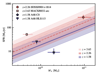
Figure 1: Bands of SFR as a function of stellar mass at three different redshifts for main-sequence galaxies (Schreiber et al., 2015, shaded areas represent $\pm 1~{}\sigma$). The symbols refer to our target (main-sequence) galaxies.

Table 2: Observational information. Note: All the frequency bands are included in every observation for the same target.

Target	R.A.	Dec.	Freq. Range	Date	Timeobs	Gain cal.	Flux/BP cal.	PWVmean
galaxy	(J2000)	(J2000)	[GHz]		[hr]			[mm]
SDSS J0901+1814	09:01:22.4	+18:14:30	98.4–102.2	2019-Jan-27	0.83	J0854+2006	J0750+1231	8.8
			110.6–114.4	2019-Mar-27	0.83	J0908+1609	J0750+1231	3.7
				2019-Mar-27	0.85	J0908+1609	J0725$-$0054	3.7
MACS J0032-arc	00:32:07.776	+18:06:47.80	139.7–143.4	2018-Dec-20	1.10	J0019+2021	J0006$-$0623	2.0
			152.0–155.4	2019-Jan-24	1.13	J0019+2021	J0006$-$0623	7.1
				2019-Mar-17	1.10	J0019+2021	J0238+1636	1.9
A68-HLS115	00:37:09.503	+09:09:03.80	125.3–128.6	2018-Dec-16	0.95	J0037+1109	J0006$-$0623	4.9
			137.1–140.7	2018-Dec-17	0.95	J0037+1109	J0006$-$0623	5.1
A68-C0	00:37:07.404	+09:09:26.57	125.1–128.6	2018-Dec-17	0.95	J0037+1109	J0006$-$0623	4.2
			137.1–140.7	2018-Dec-18	0.95	J0037+1109	J0006$-$0623	4.3

Table 3: Noise levels in the maps and spectra resulting from our observations, where channel widths were binned to 15 $\rm km\,s^{-1}$.

Target	Cont. noise level	Spectral noise level
galaxy	[mJy$\cdot$beam-1]	[mJy$\cdot$beam-1]
SDSS J0901+1814	0.01	0.01
MACS J0032-arc	0.03	0.08
A68-C0	0.02	0.19
A68-HLS115	0.01	0.22

3 Observational results

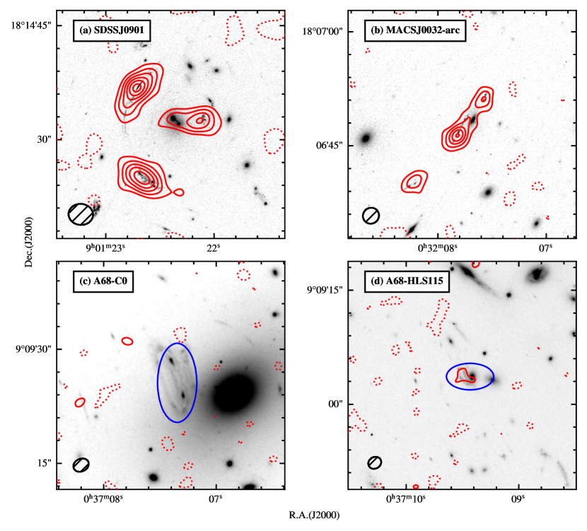
Figure 2: Millimetre continuum maps of the target galaxies. The top-left and top-right panels show HST IR images of SDSS J0901+1814 and MACS J0032-arc, respectively; the bottom left and bottom right images are for the galaxies, A68-C0 and A68-HLS115, respectively. Red solid contours indicate detection boundaries with continuum signals 3, 5, 7, 9, 11 and 13 $\times$ the noise (as calculated in CASA); red dotted lines are contours of the zero level. Black ellipses in the bottom left corners are the synthesised beam sizes for the continuum maps and the blue ellipses in the middle of the lower panels are the regions of the targets, defined manually.

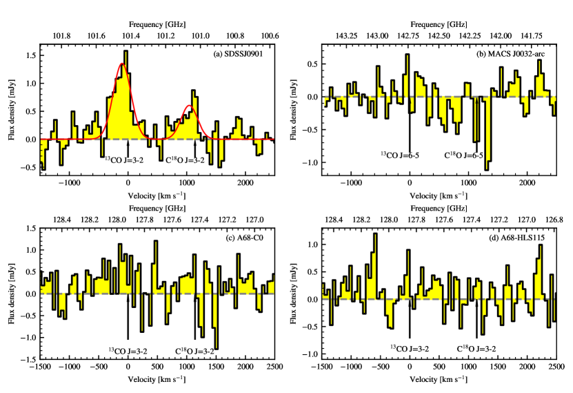
Figure 3: Spectra of ¹³CO and C¹⁸O towards our four targets. The velocity on the bottom horizontal axis is set to the velocity of ¹³CO. The spectra have been smoothed to 50 km s^-1. The grey dashed line denotes zero flux density; the red solid line is a double Gaussian fit to ¹³CO and C¹⁸O. Black arrows point to the central frequency of the ¹³CO and C¹⁸O lines.

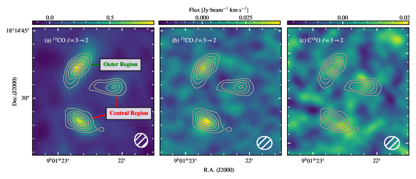
Figure 4: Images of SDSS J0901+1814. From left to right, the color maps are for the ¹²CO $J$=3$\rightarrow$2, ¹³CO $J$=3$\rightarrow$2 and C¹⁸O $J$=3$\rightarrow$2 emission lines, respectively. White contours denote 3, 5, 7, 9, 11, and 13-$\sigma$ continuum emission from our work($\sigma$ = 0.01 mJy$\cdot$beam^-1). In the ¹²COmap, the outer and central regions are labelled according to the lens modelling results in Sharon et al. (2019).

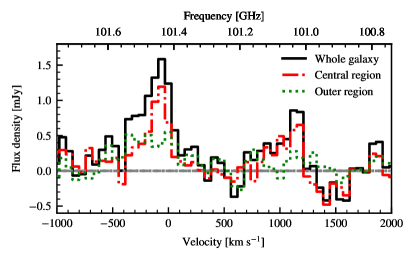
Figure 5: Spectra of ¹³CO and C¹⁸O in different parts of SDSS J0901+1814. The black-solid line represents the spectrum of the whole of SDSS J0901+1814. The red-dashed line represents the spectrum of the central region of the galaxy; the green-dotted line represents the spectrum of the outer regions of the galaxy.

3.1 Submillimeter continuum

Continuum emission from SDSS J0901+1814 and MACS J0032-arc was detected at the $>$10-$\sigma$ level, while the signal-to-noise ratios for detections of continuum towards A68-C0 and A68-HLS115 were below 5, as shown in Fig. 2.

For the two galaxies with robust continuum detections, we used their 3-$\sigma$ continuum contours as the spatial distribution over which to extract their spectrum. For the other two galaxies, we set the spatial range manually, as shown in Fig. 2 by the blue circles.

3.2 Emission lines

We have detected ¹³CO and C¹⁸O in SDSS J0901+1814, at 7.8 $\sigma$ and 3.3 $\sigma$, respectively. However, we did not detect any line emission at $>$ 3 $\sigma$ towards the other three targets. Fig. 3 shows the spatially integrated spectra of all four targets. The continuum contribution to the spectra of SDSS J0901+1814 and MACS J0032-arc have been subtracted. We did not perform continuum subtraction for A68-C0 and A68-HLS115 because there is no significant continuum emission (cf. Section 3.1). For the spectrum of SDSS J0901+1814, we fitted Gaussian profiles to the line emission (red line in Fig. 3). Fluxes and noise levels for the detected lines and continuum – along with the 3-$\sigma$ upper limits for the non-detections – are shown in Table 4. The flux ratio of ¹³CO/C¹⁸O in SDSS J0901+1814 is $2.38\pm 0.83$.

Table 4: Observational results, for lines and continuum.

Detected lines for SDSS J0901+1814
Transition	Flux	Line width (FWHM)
	[Jy km s-1]	[km s-1]
13CO $J$=3$\rightarrow$2	0.47 $\pm$ 0.06	365 $\pm$ 54
C18O  $J$=3$\rightarrow$2	0.20 $\pm$ 0.06	214 $\pm$ 83
12CO $J$=3$\rightarrow$2	8.79 $\pm$ 0.61	344 $\pm$ 7
Flux ratios of SDSS J0901+1814
$I$(13CO)/$I$(C18O)	2.38 $\pm$ 0.83
$I$(12CO)/$I$(13CO)	18.7 $\pm$ 2.7
Upper limits of 13CO and C18O
Target	Transition	3-$\sigma$ upper limit
galaxy		[Jy km s-1]
MACS J0032-arc	6–5	¡0.18
A68-C0	3–2	¡0.39
A68-HLS115	3–2	¡0.30
Continuum flux density
Target	Flux density	Frequency (obs.)
galaxy	[mJy]	[GHz]
SDSS J0901+1814	0.65 $\pm$ 0.16	106.40
MACS J0032-arc	0.82 $\pm$ 0.15	147.57
A68-C0	0.20 $\pm$ 0.16	132.91
A68-HLS115	0.17 $\pm$ 0.07	132.96

3.3 Spatial distribution of isotopologues towards SDSS J0901+1814

Fig. 4 shows the spatial distribution of the $J$=3$\rightarrow$2 transitions of ¹²CO, ¹³CO and C¹⁸O. All maps have similar beam sizes, shown in the bottom-right corner of each sub-panel. The contours show the 3-mm continuum emission, at the 3, 5, 7, 9, 11 and 13-$\sigma$ levels. For ¹²CO, the strongest of the three images is the north-eastern, while for ¹³CO it is the south-eastern. Similar to ¹²CO, the western image of ¹³CO does not show any signal above 3 $\sigma$. For C¹⁸O, the emission from all of the three images is weak. The ¹²CO and ¹³CO emission comes from well within the continuum contours. Although the western image has a 9-$\sigma$ detection of its continuum, all the line transitions show only weak emission there.

Due to the strong lensing effect (Kochanek et al., 2006), the observed galaxy images are highly distorted compared to that of the source plane. Sharon et al. (2019) performed a detailed lens modelling of SDSS J0901+1814, which appears as a single galaxy in the source plane. The velocity structure of SDSS J0901+1814 resembles a regular, rotating disk with a radius of $\sim$8 kpc, disfavoring a galaxy merger scenario.

As shown by Sharon et al. (2019), the center of SDSS J0901+1814 is transformed by lensing into the south-eastern and western images. Accordingly, we classify these two images as the central region, and the north-eastern image as the outer region. We extracted two spectra (cf. Fig. 5) from the north-eastern image, and the sum of the south-eastern and western images, respectively, thus presenting spectra of the inner and outer parts of the target galaxy. The ¹³CO/C¹⁸O ratios are $1.9\pm 1.0$ and $2.9\pm 1.2$ in the central and outer regions of the target galaxy, SDSS J0901+1814, respectively.

4 Galactic chemical evolution (GCE) model

Following the approach of Romano et al. (2017); Zhang et al. (2018) and Romano et al. (2020), we have adopted a GCE model to analyse our observational results. We employ the open-source code, NuPyCEE (Côté et al., 2017), to simulate the chemical evolution of the targeted galaxies. Besides the observed isotopic abundance ratio, which was the main focus of Zhang et al. (2018), here we could further compare measurements of the stellar mass and oxygen abundances reported in the literature (Sharon et al., 2019). We built up chemical evolution tracks: a one-zone model with several user-defined modifications. We focus on SDSS J0901+1814, in which ¹³CO and C¹⁸O were detected. In the following, we list the key parameters adopted in the model.

4.1 Stellar IMFs

Several different IMFs were adopted in our GCE models. We modified the original NuPyCEE code to better control the customised IMFs.

The forms of the adopted IMFs were as follows:

$$\xi(m)=\frac{dN}{dm}=\left\{\begin{array}[]{ll}k_{1}\times m^{-\alpha_{1}},&0.1\leq\frac{m}{M_{\odot}}<0.5,\\ k_{2}\times m^{-\alpha_{2}},&0.5\leq\frac{m}{M_{\odot}}<1,\\ k_{2}\times m^{-\alpha_{3}},&1\leq\frac{m}{M_{\odot}}<100,\end{array}\right.$$ (1)

where $k_{1}$, $k_{2}$, and $k_{3}$ are parameters that impose continuity and normalise the IMF to 1 ${\rm M}_{\odot}$ ; $m$ is the stellar mass. The power-law indices of all four IMFs are listed in Table 5.

In this work, the ‘Milky-Way IMF’ is taken from the literature, namely Romano et al. (2017); Zhang et al. (2018); Romano et al. (2019), which adopt the IMF slopes from Scalo 1986 and Kroupa et al. 1993. The $\alpha_{3}$ slope, in particular, which is found in star-forming regions in the Solar neighbourhood (Kroupa et al., 1993), best reproduces the isotopic ratios of the Milky Way (Romano et al., 2017).

The other IMFs presented in Table 5 are the same as those in Zhang et al. (2018), except for the ‘top-heavy IMF’, which is original to this work, for which we have changed the $\alpha_{3}$ slope to 2.5. In this context, ‘top-heavy’ refers to a flatter $\alpha_{3}$ slope than that of the Milky-Way IMF.

Table 5: Parameters of the IMFs used in this work.

IMF model name	$\alpha_{1}$	$\alpha_{2}$	$\alpha_{3}$	Reference
Bottom-heavy	2.7	2.7	2.7	Zhang et al. (2018)
Milky-Way	1.3	2.2	2.7	Kroupa et al. (1993)
Top-heavy	1.3	2.1	2.5	-
Ballero	1.3	1.95	1.95	Ballero et al. (2007)

4.2 Star-formation history

The star-formation history (SFH) of SDSS J0901+1814 is constrained by several observational aspects, including the upper age limit that comes from its spectroscopic redshift, the various multi-wavelength SFR estimates, and its stellar mass (Sharon et al., 2019).

The star formation is set to start 1.9 Gyr after the Big Bang, and to last for 1 Gyr. The SFR estimated from H$\alpha$ is 14.5 ${\rm M}_{\odot}\,{\rm yr}^{-1}$, a value that is likely to be heavily influenced by dust obscuration (Sharon et al., 2019). We therefore adopt the SFR of 268 ${\rm M}_{\odot}\,{\rm yr}^{-1}$ derived from the total IR luminosity (from 8 to 1000 $\mu$m in the rest frame; Sharon et al., 2019). The two SFRs were estimated assuming the IMF of Kroupa (2001).

For all of our SDSS J0901+1814 galaxy models, we adopt a stellar mass of $9.5\times 10^{10}$ ${\rm M}_{\odot}$, derived from Spitzer/IRAC 3.6$\mu$m and 4.5 $\mu$m imaging (Saintonge et al., 2013; Sharon et al., 2019). Given the same star-formation duration of 1 Gyr, tracks with different IMFs lead to slightly different SFRs. In particular, the more top-heavy the IMF, the larger the fraction of mass locked in high-mass stars in each time interval. Given the short lifetimes of massive stars (1–30 Myr), galaxies with a top-heavy IMF have lower stellar masses after 1 Gyr of evolution; thus, to form identical stellar masses at the end of the computation, higher SFRs are required for models with more top-heavy IMFs.

We design four different histories to cover both secular evolution and the most extreme starbursts:

I) Flat SFH. In this case, the SFR has a fixed value during the 1-Gyr star-forming period. The stellar mass and the chemical abundances of the galaxy both increase smoothly.

II) Exponentially declining SFH. This is inspired by the Kennicutt-Schmidt star-formation relation (Kennicutt, 1998b) and galactic infall models (Prantzos & Silk, 1998; Spitoni et al., 2017), and it is often adopted in cosmological simulations. We specify a decreasing slope of -$10^{-9}$ ${\rm M}_{\odot}$yr^-2 for the curve, but relax the initial SFR to result in a final stellar mass of $10^{11}$ ${\rm M}_{\odot}$.

III) Exponentially increasing SFH. This resembles the typical SFH observed for local dwarf galaxies (de Boer et al., 2012). In this case, most elements/isotopes are formed in the later evolutionary stages.

IV) Recent intensive starburst SFH. This model simulates the most extreme starburst galaxies, in which the burst started around 100 Myr before the observed epoch. Owing to the short timescale, stars with masses below 4–5 ${\rm M}_{\odot}$ do not contribute to the ISM enrichment, i.e. any ¹³C enrichment is limited to stars above 5 ${\rm M}_{\odot}$.

The formation of secondary elements, such as ¹⁸O, relies highly on pre-existing metals, so their abundances are sensitive to variations in the early stages of star formation.

4.3 Stellar yield tables

We have adopted the same stellar yield tables for low-metallicity AGB stars and massive stars that were used in Romano et al. (2017) and Zhang et al. (2018). Crucially, these are capable of providing a satisfactory fit to the abundances of the CNO isotopes in the Milky Way, i.e. those for which the most accurate data exist (Romano et al., 2017). For metal-rich AGB stars, we use the state-of-the-art stellar yield table from Cinquegrana & Karakas (2022). To construct the whole yields table, covering all metallicity and stellar mass ranges, we use the same methods adopted in Romano et al. (2017) and Zhang et al. (2018), where some details are elaborated as follows:

For massive stars, we adopt the supernova yields from Nomoto et al. (2013) in the mass range 13–40 ${\rm M}_{\odot}$. For AGB stars with an initial mass of 1–6.5 ${\rm M}_{\odot}$, born with relatively low metallicities ($Z\leq 0.02$), we adopt the yields from Karakas (2010). For the stellar mass range, 6.5–8 ${\rm M}_{\odot}$, at low metallicities, the stellar yields are kept equal to those of 6.5-${\rm M}_{\odot}$ stars. For AGB stars with initial masses of 1–8 ${\rm M}_{\odot}$, born with relatively high metallicities ($0.02<Z<0.05$), we adopt the yields from Cinquegrana & Karakas (2022). In the gap between 8 and 13 ${\rm M}_{\odot}$, we interpolate the stellar yields linearly on the logarithmic scale in stellar mass and metallicity. Lastly, for the mass range, 40–100 ${\rm M}_{\odot}$, we adopt the stellar yields of 40 ${\rm M}_{\odot}$ stars, the most massive in Nomoto et al. (2013). Type Ia supernovae (SN) are not considered because the yield contributions to ¹³C and ¹⁸O in Type Ia SN are below $10^{-5}\times$ those of their main isotopes (Seitenzahl et al., 2013).

4.4 IMF-weighted stellar yields

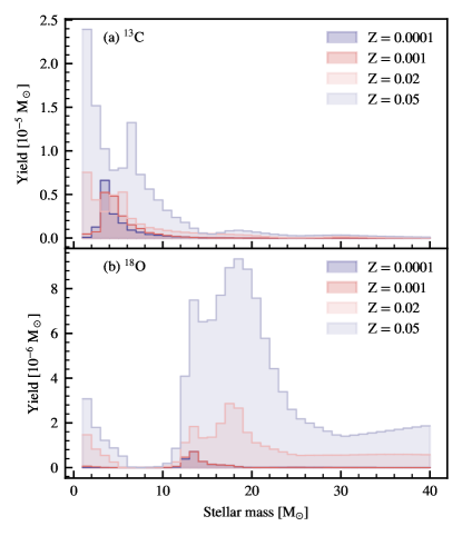
Figure 6: IMF-weighted yields (weighted by the Milky-Way IMF) for ¹³C and ¹⁸O in single stellar populations with different metallicities, represented by different colors. Contribution ratios for different types of stars are summarised in Table 6. At metallicities of 0.001 and 0.0001, the stellar yields of ¹⁸O show only very small differences across the stellar mass range.

Table 6: Production ratio of isotopes from Low-and-Intermediate Mass Stars (LIMS, M $<8$ ${\rm M}_{\odot}$) and massive stars ($M\geq 8$ ${\rm M}_{\odot}$) for a single stellar population following the Milky-way IMF. The mass of the stellar population is normalized to 1 ${\rm M}_{\odot}$. The IMF adopted for weighting is the Milky-Way IMF shown in Table 5. Here, metallicity (Z), presents the mass fraction of the elements heavier than hydrogen and helium.

Nuclei	Z	LIMS (%)	Massive stars (%)	Total yield (${\rm M}_{\odot}$)
13C	0.0001	92.9	7.1	2.4 $\times 10^{-5}$
	0.001	92.0	8.0	2.8 $\times 10^{-5}$
	0.02	84.8	15.2	6.1 $\times 10^{-5}$
	0.05	84.4	15.6	1.8 $\times 10^{-4}$
18O	0.0001	1.0	99.0	1.8 $\times 10^{-6}$
	0.001	10.1	89.9	2.1 $\times 10^{-6}$
	0.02	21.9	78.1	2.9 $\times 10^{-5}$
	0.05	14.1	85.9	2.1 $\times 10^{-4}$

Fig. 6 shows the adopted ¹³C and ¹⁸O stellar yields (Karakas, 2010; Nomoto et al., 2013; Cinquegrana & Karakas, 2022) of a single stellar population (from Section 4.3), weighted by the Milky-Way IMF (Kroupa et al., 1993) . For comparison, the masses of the stellar populations are all normalised to 1 ${\rm M}_{\odot}$. Fig. 6 shows that most of the ¹³C is produced by LIMS while most of the ¹⁸O is produced by massive stars. The specific production ratios also depend on the metallicity, $Z$, where we choose four metallicities to calculate the ratios, as shown in Table 6.

For all metallicities, over 80% of ¹³C comes from LIMS, and over 75% of ¹⁸O comes from massive stars. This strong differential explains why the mass ratio of ¹³C/¹⁸O is so sensitive to the IMF. The total production masses of ¹³C and ¹⁸O both increase with metallicity. The production of ¹⁸O, as a purely secondary element, is more sensitive to metallicity, compared with that of ¹³C  as mentioned later in Section 6.1. Single stellar populations produce a higher proportion of ¹⁸O with a top-heavy IMF than with the Milky-Way IMF. The major origin of ¹³C is stars at around 3 ${\rm M}_{\odot}$, whose lifetimes are around 200 Myr, while for ¹⁸O it is 18-${\rm M}_{\odot}$ stars with lifetimes of around 10 Myr.

4.5 Stellar mass evolution

All models have the same mass of living stars at the epoch that we have observed in the targeted galaxy, i.e. at $z=2.26$ for SDSS J0901+1814. However, NuPyCEE was not able to calculate the mass of the living stars. Therefore, we make a user-defined model to trace the stellar mass evolution, namely, stellar_evol (Guo, 2024). This code is available in the Zenodo repository: doi:10.5281/zenodo.11118895, and is also available on github. This model considers the IMF and stellar lifetimes, and it enables the derivation of the mass of living stars at any given evolutionary epoch.

4.6 Miscellaneous

Our stellar lifetime table was taken from Schaller et al. (1992), to be consistent with the stellar lifetimes implemented in the models by Romano et al. (2017) which are used in Zhang et al. (2018). In this table, the shortest lifetime is around 4 Myr for 50-${\rm M}_{\odot}$ stars. The default evolution in NuPyCEE is processed on a logarithmic scale, which cannot precisely model the chemical evolution at the later stages of the galaxy evolution. Therefore, we track the evolution on a linear scale with a fixed timestep of 4 Myr. This ensures that newly formed, massive stars and their returned stellar yields are accounted for properly.

Compared to the modelling work in Zhang et al. (2018), our work adopts a different GCE framework, NuPyCEE, slightly different stellar yield tables, a fixed evolutionary timestep setting, and without using the Q-matrix(Talbot & Arnett, 1973). However, by adopting the same SFH and IMF as Zhang et al. (2018), we can obtain the same ratio of ¹³C/¹⁸O and almost identical evolutionary tracks. This is re-assuring in terms of the robustness of our user-defined code modification.

5 Comparison of observations with GCE models

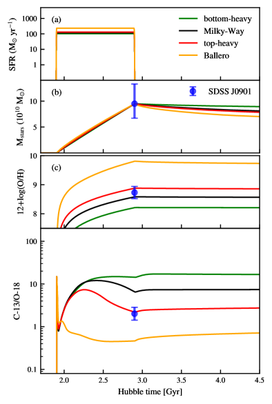
Figure 7: Predicted evolutionary tracks of the ¹³C/¹⁸O abundance ratio for galaxies with different IMFs, produced using NuPyCEE. Green curves are the GCE results assuming the bottom-heavy IMF; black curves assume the Milky-Way IMF (Kroupa et al., 1993); red curves assume the top-heavy IMF; yellow curves assume the Ballero IMF. Blue circles are the observed stellar mass and oxygen abundance in SDSS J0901+1814, adopted from Sharon et al. (2019). The parameters of all the IMFs are listed in Table 5 and the SFR is IMF-dependent.

Fig. 7 presents a comparison between our observed line ratio, from Section 3, and the GCE model predictions, as described in Section 4. The curves show the evolutionary tracks of SFR, stellar mass, oxygen abundance and ¹³C/¹⁸O ratios for models corresponding to our different adopted IMFs, from bottom-heavy to top-heavy. All SFR tracks have the same slope, the same star-formation duration, and the same final stellar mass, as mentioned in Section 4.2.

The stellar masses of all models reach $9.5\times 10^{10}$ ${\rm M}_{\odot}$ after 3 Gyr, as we required. After the cessation of star formation, the stellar masses start to decrease slowly. The stellar mass of the model with the most top-heavy IMF falls fastest, because it has the highest fraction of short-lived massive stars.

The oxygen abundances of all models increase rapidly after the star formation starts and continues to increase monotonically until the star formation ceases. After that, the oxygen abundance of all models remains stable. The models with the most top-heavy IMFs tend to end with higher oxygen abundance.

During the first 50–100 Myr of star formation, the ¹³C/¹⁸O abundance ratio increases first, and then decreases rapidly, for all models. After the lowest dip, the isotopic ratios of all models, except the one with the Ballero IMF, increase slowly to its second peak value and then decrease gradually. The Ballero-IMF model has a small bump and decreases rapidly until star formation ceases.

The ¹³C/¹⁸O ratio agrees with the model that assumes a top-heavy IMF; it cannot be explained by the other three IMFs (including the Milky-Way IMF). Under the Milky-Way IMF, our ¹³C/¹⁸O evolutionary track is roughly consistent with that in Zhang et al. (2018), which is optimised for starburst galaxies. The observed oxygen abundance (12+log(O/H)) can match both the Kroupa and the top-heavy IMFs; the other two IMFs do not match.

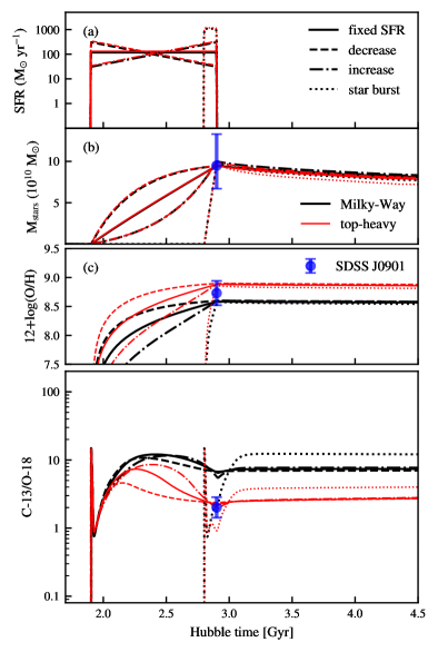
Figure 8: Theoretical predictions for the ¹³C/¹⁸O abundance ratio: evolutionary tracks of galaxies with different SFHs are shown by different line styles. Solid lines are the constant SFR model, which is the same as the SFH of Fig. 7. Dashed lines are the decreasing SFH; dash-dotted lines are the increasing SFH; dotted lines are the intense starburst SFH. Different line styles represent different IMFs implied in the models. Black curves represent the Milky-Way IMF (Kroupa et al., 1993); red curves represent the top-heavy IMF (defined in Table 5). Blue dots represent our observations of SDSS J0901+1814.

As described in Section 4.2, we assume four different SFHs, aiming to break the degeneracy between the SFH and IMF. The oxygen abundance can be explained by both the Milky-Way and the top-heavy IMFs, leaving some ambiguity, so it is necessary to test whether an extreme SFH with a Milky-Way IMF could achieve the observed ¹³C/¹⁸O ratio.

We investigated eight models, which consist of two different IMFs – the Milky-Way and top-heavy IMFs, and four different SFHs, to trace the evolution of SFR, stellar mass, oxygen abundance and ¹³C/¹⁸O ratios. These models are presented in Fig. 8.

In Fig. 8, all model tracks show strong variations due to the IMF, no matter which SFH is adopted. Although different SFHs would introduce individual biased evolutionary tracks, all models are designed to reproduce the same stellar mass at the epoch when we observe SDSS J0901+1814. Varying the SFH does not have a strong impact on the oxygen abundances, which are more sensitive to the choice of IMF; all predicted oxygen abundances are within 1-$\sigma$ of the observational data for SDSS J0901+1814.

Measurements of the stellar mass and the oxygen abundance help to reinforce the constraints from the GCE modelling, compared to the dusty starburst galaxies observed in Zhang et al. (2018). Taken alone, the oxygen abundance is not enough to discriminate between the IMFs, but only the models with a top-heavy IMF can explain the observed ¹³C/¹⁸O ratio. No matter which SFH is applied in the model, the observed ¹³C/¹⁸O value cannot be reproduced with the Milky-Way IMF within the observational uncertainties.

6 Discussion

6.1 The influence of the star-formation history

As shown in Fig. 8, the SFH only slightly influences the evolution of ¹³C/¹⁸O, for the following reasons:

First, the ratio between the stellar yield of ¹³C and ¹⁸O relies strongly on the initial metallicity of the stars (e.g. Wiescher et al., 2010). As demonstrated in Section 4.4 and Fig. 6, contribution ratios of ¹³C and ¹⁸O all rely on metallicity. Compared to ¹³C, the stellar yield of ¹⁸O is more sensitive to metallicity, because ¹³C is both a primary and a secondary element, which can be produced by the first generation of stars. On the other hand, ¹⁸O is a pure secondary element and can only be produced by stars containing ¹⁴N seeds at the moment the star was born (Wilson & Matteucci, 1992; Romano et al., 2017). Most ¹⁸O is therefore produced in the late, metal-rich stage of galaxy evolution. It is this timing discrepancy which leads to the differences in the chemical enrichment of ¹³C and ¹⁸O.

For all models in Figs. 7 and 8, the ¹³C/¹⁸O abundance ratios start from a high level in the earliest few Myrs, quickly drop, then present an increasing trend. In this phase, a low ¹³C/¹⁸O ratio can persist for $\lesssim$ 100 Myr, during which the galaxy is still very metal-poor and most ¹³C is not yet released to the ISM. At this early evolutionary stage, both stellar mass and metallicity are orders of magnitude lower than the final, observed values.

Second, the release times of ¹³C and ¹⁸O are different. ¹³C and ¹⁸O are mostly produced by LIMS and massive stars, which have longer and shorter stellar lifetimes (Schaller et al., 1992), respectively. After the initial drop (see Fig. 7 (d)), the abundance ratio of ¹³C/¹⁸O increases slowly as the galaxy evolves and the ¹³C is released gradually by LIMS.

Third, if the star-formation timescale is longer than 2 Gyr, the contribution of novae becomes non-negligible (Dantona & Mazzitelli, 1982; Romano et al., 1999; Romano & Matteucci, 2003). However, nova outbursts mainly enrich isotopic abundances of ¹³C, ¹⁵N and ¹⁷O (Starrfield et al., 1972, 1974; Romano & Matteucci, 2003), compared to that of ¹⁸O. Including the contribution of novae would thus reinforce our conclusion that the IMF must be top-heavy, since it would increase the ¹³C/¹⁸O ratio in the models.

With a Milky-Way IMF, only if such a massive galaxy is formed over a timescale shorter than 100 Myr, where the corresponding SFR is above 1000 ${\rm M}_{\odot}\,{\rm yr}^{-1}$, could the ¹³C/¹⁸O ratio match the observed value. This is demonstrated by the starburst model in Fig. 8, in which a flat burst history with an SFR of 1000 ${\rm M}_{\odot}\,{\rm yr}^{-1}$ results in a ¹³C/¹⁸O ratio of $\sim 2$, below the other SFH tracks with the Milky-Way IMF.

With the same IMF, a single starburst model would predict a slightly higher (within a factor of $2\times$) ¹³C/¹⁸O ratio at the evolutionary end point, compared to those produced with other more slowly-evolving SFHs, as shown in Fig. 8. This is because most stars were formed quickly in low-metallicity conditions. Given the relatively low production of ¹⁸O from massive stars at low metallicities, as shown in Fig. 6, the final ¹³C/¹⁸O ratio could be slightly increased. This small difference would not affect our main results.

6.2 Spatial distribution of the IMF

Aided by strong lensing, we can partially resolve the spatial distribution of SDSS J0901+1814. As shown in Section 3.3, ¹³CO/C¹⁸O isotopologue flux ratios show differences amongst the three lensed images. The line ratio from the outer region is slightly higher than that of the galactic center. This indicates that the IMF in the central region might be more top-heavy than that in the outer region.

If confirmed, this phenomenon would be in line with the integrated galactic IMF (IGIMF) theory (Kroupa & Weidner, 2003; Weidner & Kroupa, 2005; Kroupa et al., 2013). In that theory, both the slope of the mass function of the embedded clusters and the IMF rely on the SFR (Yan et al., 2017). In Sharon et al. (2019), the SFR of SDSS J0901+1814 shows a decreasing radial distribution, consistent with spiral galaxies in the local Universe (González Delgado et al., 2016), in both the image and the source plane. Since the SFR density is highest in the galaxy center, the final integrated IMF would also be most top-heavy in that same central region. However, the sensitivity of the current data is somewhat limited, and we merely regard the observed spatial variation of the IMF in SDSS J0901+1814 as a plausible scenario, in need of confirmation.

6.3 Impact on the cosmic evolution of star formation

Variations of the IMF can affect measurements of the SFR, because most SFR tracers – ultraviolet radiation, H$\alpha$ emission, total infrared luminosity, etc. – are linked to the effects of massive, young stars (e.g. Kennicutt, 1998b). If the IMF in a galaxy deviates from that seen in the Milky Way, which has been used to benchmark most SFR tracers (Kennicutt, 1998b), then the SFR deduced for that galaxy will be systematically in error. Our work implies that the IMF in high-redshift main-sequence galaxies, which are believed to dominate the SFR density at and around ‘cosmic noon’ ($z\approx 1$–3), is more top-heavy than the IMF of the Milky Way. These galaxies thus contain a higher fraction of massive stars than the Milky Way, and therefore produce a higher luminosity per unit stellar mass in ultraviolet radiation, H$\alpha$ emission, total infrared luminosity, etc., meaning that their real SFRs (and total stellar masses) are likely rather lower than those calculated in the literature to date (Jeřábková et al., 2018).

With stellar_evol we estimate the proportion of massive stars among all living stars in our simulations, for different assumed IMFs. For the same total stellar mass, the fraction by mass of massive stars for the Milky-Way IMF and the top-heavy IMF are 1.5‰ and 2.5‰, respectively. Thus if main-sequence galaxies at high redshift – as represented by SDSS J0901+1814 – have top-heavy IMFs, then their SFR estimates could decrease by more than 40%, consistent with recent findings using the James Webb Space Telescope in high-redshift galaxies (Inayoshi et al., 2022; Wang et al., 2023, cf. Cullen et al. 2023).

More detailed calculations and benchmarking for SFR tracers are beyond the scope of this work.

7 Summary

In this paper, we report observations of CO isotopologues in four strongly lensed main-sequence galaxies at redshift $\sim 2$. A robust detection of ¹³CO and C¹⁸O emission is obtained from one target, SDSS J0901+1814, at $z\sim 2.26$. This is the first detection of CO isotopologues in a main-sequence galaxy at high redshift. The observed flux ratio of ¹³CO/C¹⁸O in this galaxy is $2.4\pm 0.8$, which is lower than the average value observed for local main-sequence galaxies. Via detailed galactic chemical evolution modelling, we find that only an IMF more top-heavy than the Milky Way IMF can reproduce the observed isotopic ratio, oxygen abundance, and stellar mass, simultaneously. The power-law indices of Milky Way IMF and the top-heavy IMF differ by only a small amount of 0.2, which already changes the ¹³C/¹⁸O ratio by a factor of 3–4$\times$, which showcases the sensitivity of the isotopic method. Our result suggests that main-sequence galaxies in the high-redshift Universe may prefer a top-heavy IMF, and therefore, create more massive stars than previously thought.

References

- Ballero et al. (2007) Ballero, S. K., Matteucci, F., Origlia, L., & Rich, R. M. 2007, A&A, 467, 123, doi: 10.1051/0004-6361:20066596
- Bastian et al. (2010) Bastian, N., Covey, K. R., & Meyer, M. R. 2010, ARA&A, 48, 339, doi: 10.1146/annurev-astro-082708-101642
- Baugh et al. (2005) Baugh, C. M., Lacey, C. G., Frenk, C. S., et al. 2005, MNRAS, 356, 1191, doi: 10.1111/j.1365-2966.2004.08553.x
- Brown & Wilson (2019) Brown, T., & Wilson, C. D. 2019, ApJ, 879, 17, doi: 10.3847/1538-4357/ab2246
- Cinquegrana & Karakas (2022) Cinquegrana, G. C., & Karakas, A. I. 2022, MNRAS, 510, 1557, doi: 10.1093/mnras/stab3379
- Conselice (2014) Conselice, C. J. 2014, ARA&A, 52, 291, doi: 10.1146/annurev-astro-081913-040037
- Côté et al. (2017) Côté, B., O’Shea, B. W., Ritter, C., Herwig, F., & Venn, K. A. 2017, ApJ, 835, 128, doi: 10.3847/1538-4357/835/2/128
- Cullen et al. (2023) Cullen, F., McLeod, D. J., McLure, R. J., et al. 2023, arXiv e-prints, arXiv:2311.06209, doi: 10.48550/arXiv.2311.06209
- Daddi et al. (2007) Daddi, E., Dickinson, M., Morrison, G., et al. 2007, ApJ, 670, 156, doi: 10.1086/521818
- Danielson et al. (2013) Danielson, A. L. R., Swinbank, A. M., Smail, I., et al. 2013, MNRAS, 436, 2793, doi: 10.1093/mnras/stt1775
- Dantona & Mazzitelli (1982) Dantona, F., & Mazzitelli, I. 1982, ApJ, 260, 722, doi: 10.1086/160292
- de Boer et al. (2012) de Boer, T. J. L., Tolstoy, E., Hill, V., et al. 2012, A&A, 539, A103, doi: 10.1051/0004-6361/201118378
- Dessauges-Zavadsky et al. (2015) Dessauges-Zavadsky, M., Zamojski, M., Schaerer, D., et al. 2015, A&A, 577, A50, doi: 10.1051/0004-6361/201424661
- Dessauges-Zavadsky et al. (2017) Dessauges-Zavadsky, M., Zamojski, M., Rujopakarn, W., et al. 2017, A&A, 605, A81, doi: 10.1051/0004-6361/201628513
- Elmegreen et al. (2008) Elmegreen, B. G., Bournaud, F., & Elmegreen, D. M. 2008, ApJ, 688, 67, doi: 10.1086/592190
- Geha et al. (2013) Geha, M., Brown, T. M., Tumlinson, J., et al. 2013, ApJ, 771, 29, doi: 10.1088/0004-637X/771/1/29
- Giannetti et al. (2014) Giannetti, A., Wyrowski, F., Brand, J., et al. 2014, A&A, 570, A65, doi: 10.1051/0004-6361/201423692
- González Delgado et al. (2016) González Delgado, R. M., Cid Fernandes, R., Pérez, E., et al. 2016, A&A, 590, A44, doi: 10.1051/0004-6361/201628174
- Gunawardhana et al. (2011) Gunawardhana, M. L. P., Hopkins, A. M., Sharp, R. G., et al. 2011, MNRAS, 415, 1647, doi: 10.1111/j.1365-2966.2011.18800.x
- Guo (2024) Guo, Z.-Y. 2024, GuoZiYi-astro/stellar_evol: v0.0.0, v0.0.0, Zenodo, doi: 10.5281/zenodo.11118896
- Henkel et al. (2014) Henkel, C., Asiri, H., Ao, Y., et al. 2014, A&A, 565, A3, doi: 10.1051/0004-6361/201322962
- Hopkins (2018) Hopkins, A. M. 2018, PASA, 35, e039, doi: 10.1017/pasa.2018.29
- Huang et al. (2023) Huang, R., Battisti, A. J., Grasha, K., et al. 2023, MNRAS, 520, 446, doi: 10.1093/mnras/stad108
- Inayoshi et al. (2022) Inayoshi, K., Harikane, Y., Inoue, A. K., Li, W., & Ho, L. C. 2022, ApJ, 938, L10, doi: 10.3847/2041-8213/ac9310
- Jeřábková et al. (2018) Jeřábková, T., Hasani Zonoozi, A., Kroupa, P., et al. 2018, A&A, 620, A39, doi: 10.1051/0004-6361/201833055
- Jiménez-Donaire et al. (2017) Jiménez-Donaire, M. J., Cormier, D., Bigiel, F., et al. 2017, ApJ, 836, L29, doi: 10.3847/2041-8213/836/2/L29
- Karakas (2010) Karakas, A. I. 2010, MNRAS, 403, 1413, doi: 10.1111/j.1365-2966.2009.16198.x
- Kennicutt (1998a) Kennicutt, Robert C., J. 1998a, ApJ, 498, 541, doi: 10.1086/305588
- Kennicutt (1998b) —. 1998b, ARA&A, 36, 189, doi: 10.1146/annurev.astro.36.1.189
- Kobayashi et al. (2011) Kobayashi, C., Karakas, A. I., & Umeda, H. 2011, MNRAS, 414, 3231, doi: 10.1111/j.1365-2966.2011.18621.x
- Kochanek et al. (2006) Kochanek, C. S., Schneider, P., & Wambsganss, J. 2006, Part 2 of Gravitational Lensing: Strong, Weak and Micro, doi: 10.48550/arXiv.astro-ph/0407232
- Kroupa (2001) Kroupa, P. 2001, MNRAS, 322, 231, doi: 10.1046/j.1365-8711.2001.04022.x
- Kroupa et al. (1993) Kroupa, P., Tout, C. A., & Gilmore, G. 1993, MNRAS, 262, 545, doi: 10.1093/mnras/262.3.545
- Kroupa & Weidner (2003) Kroupa, P., & Weidner, C. 2003, ApJ, 598, 1076, doi: 10.1086/379105
- Kroupa et al. (2013) Kroupa, P., Weidner, C., Pflamm-Altenburg, J., et al. 2013, The Stellar and Sub-Stellar Initial Mass Function of Simple and Composite Populations, ed. T. D. Oswalt & G. Gilmore, Vol. 5, 115, doi: 10.1007/978-94-007-5612-0_4
- Lee et al. (2009) Lee, J. C., Gil de Paz, A., Tremonti, C., et al. 2009, ApJ, 706, 599, doi: 10.1088/0004-637X/706/1/599
- Li et al. (2023) Li, J., Liu, C., Zhang, Z.-Y., et al. 2023, Nature, 613, 460, doi: 10.1038/s41586-022-05488-1
- Madau & Dickinson (2014) Madau, P., & Dickinson, M. 2014, ARA&A, 52, 415, doi: 10.1146/annurev-astro-081811-125615
- Marigo (2001) Marigo, P. 2001, A&A, 370, 194, doi: 10.1051/0004-6361:20000247
- Matteucci (2001) Matteucci, F. 2001, The chemical evolution of the Galaxy, Vol. 253, doi: 10.1007/978-94-010-0967-6
- Matteucci & Brocato (1990) Matteucci, F., & Brocato, E. 1990, ApJ, 365, 539, doi: 10.1086/169508
- McMullin et al. (2007) McMullin, J. P., Waters, B., Schiebel, D., Young, W., & Golap, K. 2007, in Astronomical Society of the Pacific Conference Series, Vol. 376, Astronomical Data Analysis Software and Systems XVI, ed. R. A. Shaw, F. Hill, & D. J. Bell, 127
- Mucciarelli et al. (2021) Mucciarelli, A., Massari, D., Minelli, A., et al. 2021, Nature Astronomy, 5, 1247, doi: 10.1038/s41550-021-01493-y
- Nomoto et al. (2013) Nomoto, K., Kobayashi, C., & Tominaga, N. 2013, ARA&A, 51, 457, doi: 10.1146/annurev-astro-082812-140956
- Papadopoulos et al. (2011) Papadopoulos, P. P., Thi, W.-F., Miniati, F., & Viti, S. 2011, MNRAS, 414, 1705, doi: 10.1111/j.1365-2966.2011.18504.x
- Pettini & Pagel (2004) Pettini, M., & Pagel, B. E. J. 2004, MNRAS, 348, L59, doi: 10.1111/j.1365-2966.2004.07591.x
- Planck Collaboration et al. (2016) Planck Collaboration, Ade, P. A. R., Aghanim, N., et al. 2016, A&A, 594, A13, doi: 10.1051/0004-6361/201525830
- Portinari et al. (1998) Portinari, L., Chiosi, C., & Bressan, A. 1998, A&A, 334, 505. https://arxiv.org/abs/astro-ph/9711337
- Prantzos & Silk (1998) Prantzos, N., & Silk, J. 1998, ApJ, 507, 229, doi: 10.1086/306327
- Rieke et al. (1993) Rieke, G. H., Loken, K., Rieke, M. J., & Tamblyn, P. 1993, ApJ, 412, 99, doi: 10.1086/172904
- Ritter et al. (2018) Ritter, C., Côté, B., Herwig, F., Navarro, J. F., & Fryer, C. L. 2018, ApJS, 237, 42, doi: 10.3847/1538-4365/aad691
- Romano (2022) Romano, D. 2022, A&A Rev., 30, 7, doi: 10.1007/s00159-022-00144-z
- Romano & Matteucci (2003) Romano, D., & Matteucci, F. 2003, MNRAS, 342, 185, doi: 10.1046/j.1365-8711.2003.06526.x
- Romano et al. (1999) Romano, D., Matteucci, F., Molaro, P., & Bonifacio, P. 1999, A&A, 352, 117, doi: 10.48550/arXiv.astro-ph/9910151
- Romano et al. (2019) Romano, D., Matteucci, F., Zhang, Z.-Y., Ivison, R. J., & Ventura, P. 2019, MNRAS, 490, 2838, doi: 10.1093/mnras/stz2741
- Romano et al. (2017) Romano, D., Matteucci, F., Zhang, Z. Y., Papadopoulos, P. P., & Ivison, R. J. 2017, MNRAS, 470, 401, doi: 10.1093/mnras/stx1197
- Romano et al. (2020) Romano, D., Zhang, Z.-Y., Matteucci, F., Ivison, R. J., & Papadopoulos, P. P. 2020, in Uncovering Early Galaxy Evolution in the ALMA and JWST Era, ed. E. da Cunha, J. Hodge, J. Afonso, L. Pentericci, & D. Sobral, Vol. 352, 234–238, doi: 10.1017/S174392131900886X
- Saintonge et al. (2013) Saintonge, A., Lutz, D., Genzel, R., et al. 2013, ApJ, 778, 2, doi: 10.1088/0004-637X/778/1/2
- Scalo (1986) Scalo, J. M. 1986, Fund. Cosmic Phys., 11, 1
- Schaller et al. (1992) Schaller, G., Schaerer, D., Meynet, G., & Maeder, A. 1992, A&AS, 96, 269
- Schneider et al. (2018) Schneider, F. R. N., Sana, H., Evans, C. J., et al. 2018, Science, 359, 69, doi: 10.1126/science.aan0106
- Schreiber et al. (2015) Schreiber, C., Pannella, M., Elbaz, D., et al. 2015, A&A, 575, A74, doi: 10.1051/0004-6361/201425017
- Seitenzahl et al. (2013) Seitenzahl, I. R., Ciaraldi-Schoolmann, F., Röpke, F. K., et al. 2013, MNRAS, 429, 1156, doi: 10.1093/mnras/sts402
- Sharon et al. (2019) Sharon, C. E., Tagore, A. S., Baker, A. J., et al. 2019, ApJ, 879, 52, doi: 10.3847/1538-4357/ab22b9
- Sliwa et al. (2017) Sliwa, K., Wilson, C. D., Aalto, S., & Privon, G. C. 2017, ApJ, 840, L11, doi: 10.3847/2041-8213/aa6ea4
- Smith (2020) Smith, R. J. 2020, ARA&A, 58, 577, doi: 10.1146/annurev-astro-032620-020217
- Spitoni et al. (2017) Spitoni, E., Gioannini, L., & Matteucci, F. 2017, A&A, 605, A38, doi: 10.1051/0004-6361/201730545
- Starrfield et al. (1974) Starrfield, S., Sparks, W. M., & Truran, J. W. 1974, ApJS, 28, 247, doi: 10.1086/190317
- Starrfield et al. (1972) Starrfield, S., Truran, J. W., Sparks, W. M., & Kutter, G. S. 1972, ApJ, 176, 169, doi: 10.1086/151619
- Talbot & Arnett (1973) Talbot, Raymond J., J., & Arnett, W. D. 1973, ApJ, 186, 51, doi: 10.1086/152477
- van der Giessen et al. (2022) van der Giessen, S. A., Leslie, S. K., Groves, B., et al. 2022, A&A, 662, A26, doi: 10.1051/0004-6361/202142452
- Wang et al. (2023) Wang, Y.-Y., Lei, L., Yuan, G.-W., & Fan, Y.-Z. 2023, arXiv e-prints, arXiv:2307.12487, doi: 10.48550/arXiv.2307.12487
- Weidner & Kroupa (2005) Weidner, C., & Kroupa, P. 2005, ApJ, 625, 754, doi: 10.1086/429867
- Wiescher et al. (2010) Wiescher, M., Görres, J., Uberseder, E., Imbriani, G., & Pignatari, M. 2010, Annual Review of Nuclear and Particle Science, 60, 381, doi: 10.1146/annurev.nucl.012809.104505
- Wilson & Matteucci (1992) Wilson, T. L., & Matteucci, F. 1992, A&A Rev., 4, 1, doi: 10.1007/BF00873568
- Yan et al. (2017) Yan, Z., Jerabkova, T., & Kroupa, P. 2017, A&A, 607, A126, doi: 10.1051/0004-6361/201730987
- Yan et al. (2020) —. 2020, A&A, 637, A68, doi: 10.1051/0004-6361/202037567
- Yang et al. (2023) Yang, C., Omont, A., Martín, S., et al. 2023, A&A, 680, A95, doi: 10.1051/0004-6361/202347610
- Yoast-Hull et al. (2016) Yoast-Hull, T. M., Gallagher, J. S., & Zweibel, E. G. 2016, MNRAS, 457, L29, doi: 10.1093/mnrasl/slv195
- Zhang et al. (2018) Zhang, Z.-Y., Romano, D., Ivison, R. J., Papadopoulos, P. P., & Matteucci, F. 2018, Nature, 558, 260, doi: 10.1038/s41586-018-0196-x