Characterizing Asymptotic Expansions of Quantum Fermi Gas

Abstract

We characterize in a novel manner the physical properties of the low temperature Fermi gas in the degenerate domain as a function of temperature and chemical potential. For the first time we obtain low temperature $T$ results in the domain where several fermions are found within a de Broglie spatial cell. In this regime, the usual high degeneracy Sommerfeld expansion fails. The other known semi-classical Boltzmann domain applies when fewer than one particle is found in the de Broglie cell. The relative errors of the three approximate methods (Boltzmann limit, Sommerfeld expansion, and the new domain of several particles in the de Broglie cell) are quantified. In order to extend the understanding of the Sommerfeld expansion, we developed a novel characterization of the Fermi distribution allowing the separation of the finite and zero temperature phenomena.

1 Introduction

1.1 Motivation

Many interesting effects related to the Pauli principle appear at finite, but low temperatures, in vastly different physical systems [1, 2, 3, 4]. The limit $T\to 0$ of the Fermi-Dirac (FD) quantum system is subtle. We show analytical results which depend on particle number density within the de Broglie volume $V_{\mathrm{dB}}$, in $D$-dimensions defined by

$$V_{\mathrm{dB}}=L_{\mathrm{dB}}^{D},\qquad L_{\mathrm{dB}}=\frac{2\pi\hbar}{\langle p\rangle_{T}},\qquad\langle p\rangle_{T}=\left\langle\sqrt{E^{2}-m^{2}}\ \right\rangle_{T}\;,$$ (1)

where angle brackets denote thermal averages. Any physical systems maintaining a prescribed particle number density in the $T\to 0$ limit requires a simultaneous chemical potential $\mu$ limit. For this reason, key physical features of low-temperature FD quantum gasses can be missed if the appropriate relation between $\mu$ and $T$ is not maintained in the low temperature limit. In this work, we show that a careful treatment of the simultaneous limit leads to novel asymptotic expansions of FD thermal averages. While in principle this is not an unexpected finding, we have found no mention of such mathematical considerations in literature.

The asymptotic limit of integrals of the FD distribution [5, 6] are of interest to physicists studying many diverse statistical quantum systems [7, 8, 9, 10, 11, 12] and behavior around the Fermi surface [13, 14]. Other use cases include compact astrophysical systems (white dwarfs, neutron stars, quark stars) [15, 3, 16], Early Universe phenomenology [17, 18, 19, 20], quark-gluon plasmas (QGP) [2, 21, 22, 23], and in any situation when finite temperature Fermi effects are important. When investigating the low temperature limit of a Fermi gas, a systematic approach to approximating the physical integral involves employs the Sommerfeld expansion. It is worth noting that the Sommerfeld expansion, as described in Ref. [24], is asymptotic in nature. It is within this context that we often see matter-of-fact statements that the “Sommerfeld expansion fails” in various regimes. A textbook example is seen on page 38 of Ref. [4] (for the Sommerfeld expansion in this text, see p. 24). However, there appears to have been no progress towards a wholly distinct expansion which could rectify this issue. This situation seems to have lasted now for nearly a century.

After several in-depth reviews of literature, we conclude that a full understanding of the domain of validity of the Sommerfeld expansion in the $(T,\Delta\mu)$-plane

$$\Delta\mu\equiv\mu-m\,,$$ (2)

is lacking. The Sommerfeld expansion fails for regimes where the corrections to the $T\rightarrow 0$ limit cannot be taken to be small. This makes it difficult to search for alternative expansions that are valid in other regions of the $(T,\Delta\mu)$-plane when dealing with multiple scales. One generally requires specialized asymptotic expansions that are adapted to specific regimes under consideration. This is particularly relevant when $\Delta\mu$ is small, a regime that the traditional Sommerfeld expansion was not designed for and which we consider here. Specifically, expanding the Sommerfeld result around the small chemical potential may lead to encountering singularities which underscore the necessity for a better tool to study this scenario.

In this work we explore the different domains of low temperature FD gas, characterize the domain of validity of Sommerfeld expansion in physical terms, and obtain a novel approximation applicable to domains of statistical parameters where the “expansion fails”. As a side-line result, we also provide a novel form of FD distribution that manifestly separates the zero and finite temperature contributions so that the finite temperature correction can be studied on its own in more complex environments than considered in our current method-oriented presentation.

Our own interest and motivations to explore FD systems originated in cosmological computations involving both high and low temperature physics, such as comic neutrino background [25, 26] and cosmic magnetism [20]. In the context of magnetism an added difficulty is the Landau discrete sum over Landau orbitals. In the regime of neutrino cosmology, considering their likely mass, the present-day free-streaming neutrinos exhibit characteristics of being cold and nonrelativistic fermions, with a small chemical potential reflecting the baryon asymmetry in the universe. During the Universe expansion neutrino abundance per quantum correlation de Broglie volume decreases. Therefore the free-streaming neutrinos might fall into the novel regime described here.

1.2 Domains of interest and their characteristic particle density

In this work we derive and contrast expansions of FD matter in the following regimes which, to the best of the authors’ knowledge, contain several novel insights. In Figure 1 we show the domains of interest in the ($T,\Delta\mu$)-plane (in units of $m$). The darker background shows regions with relative error less than $10\%$, lighter background shows error less $20\%$, when computing $\langle G\rangle_{T}$ for the illustrative choice $G(p)=1$. Errors here, and elsewhere in this work, were obtained by comparing the approximations with the result obtained from standard numerical quadrature; given the form of the FD integrand, such methods can be reliably used as long as the values of $\mu$ and $T$ are not too extreme. We also show using solid black contours lines the number of particles per de Broglie volume. From these one can recognize

1. The traditional Sommerfeld asymptotic expansion applies when statistical parameters allow for a quantum degenerate density of Fermi particles, with about 5 or more particles found in the corresponding de Broglie volume. As will be considered here the validity of this regime can be extended to the dense relativistic quantum domain.

2. The domain of validity of the newly characterized dilute quantum region (Theorem 5) is found when the combination of statistical parameters allows a moderate particle density of a few (2 to 3) particles per de Broglie volume, where quantum effects are expected to be nontrivial but different from properties of dense FD matter.

3. The Boltzmann limit applies to systems with about 1 or fewer particles per de Broglie volume,

Particle abundance described and shown in Figure 1 does not account for spin and other degeneracies. Finally we note that Figure 1 focuses on the non-relativistic domain; for a similar figure that shows the relativistic regime see Figure 6.

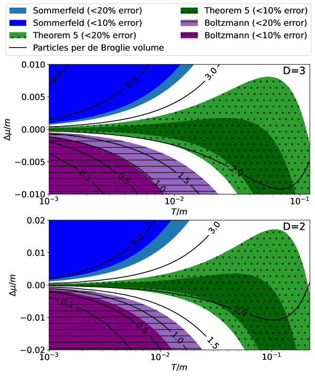
Figure 1: Domains of interest spanned in the $(T/m,\Delta\mu/m\equiv(\mu-m)/m)$-plane, top for three dimensional and bottom frame for two dimensional systems: Sommerfeld expansion (blue); Boltzmann approximation (lined purple), and the new Theorem 5 domain (dotted green). Solid black contours show the number of particles per de Broglie volume Eq. (1). See text for a more detailed discussion.

Our novel contributions include consideration of:

1. Nonrelativistic degenerate Fermi gas region (Theorem 2): Application of the traditional Sommerfeld expansion in this regime requires care, as the coefficients in the expansion can become singular when $\mu\to m$. In Section 2.3 we derive a formula that resolves those singularities so as to avoid such numerical difficulties and obtain an expansion up to a specified order. In this derivation we utilize a novel decomposition of the FD distribution into finite and zero temperature components, see Section 2.1, which we find convenient for guiding this and other derivations.

2. Degenerate relativistic Fermi gas Sommerfeld expansion (Theorem 3): We prove that the traditional Sommerfeld expansion, which applies to the regime $T\ll m$ with $\Delta\mu$ not small, also applies to the high-temperature regime $\mu\gg T\gg m$ under appropriate assumptions.

3. Dilute quantum region (DQR) (Theorem 5): We demonstrate that the Sommerfeld expansion can fail completely when $|\mu-m|\ll T\ll m$; see the example in Figure 5 below. Accurate results in this regime require the use of the new expansion that we derive in Section 3. In Figure 1 we preview the new expansion stated in Theorem 5, comparing its domain of validity to that of the Sommerfeld expansion in dimensions $D=2,3$. In particular, note that the new expansion derived here covers a distinct new region in the $(T/m,\Delta\mu/m)$-plane where just a few particles are present in a de Broglie volume.

2 Sommerfeld-Type Asymptotic Characterization of Thermal Properties

2.1 A new FD distribution decomposition

In this section we will explore the Sommerfeld-type asymptotic expansions of thermal averages in various physics-relevant chemical potential and temperature regimes. As a convenient tool, we will employ the following novel way to write FD distribution in the zero temperature limit $T\to 0$.

At $T=0$ the FD distribution reduces to a step function where a state $E_{i}$ is either filled or empty. For given chemical potential $\mu(T)$, we have

$$f_{\mathrm{FD}}[E_{i},\mu(T),T]=\frac{1}{\displaystyle e^{\left(\frac{E_{i}-\mu}{T}\right)}+1}\,,\qquad\lim_{T\to 0}f_{\mathrm{FD}}=\left\{\begin{array}[]{c}1,\quad\mathrm{for}\quad{E_{i}}<{E_{F}}\\ 0,\quad\mathrm{for}\quad{E_{i}}>{E_{F}}\end{array}\right.\,.$$ (5)

At $T=0$ the energy of the last filled state is the Fermi energy ${E_{\mathrm{F}}=\mu(T\to 0)}$, while at finite temperature one speaks of chemical potential instead.

For the calculations in this section we find it useful to employ a novel reformulation which allows exact separation of the finite temperature behavior from the singular zero temperature limit, replacing the smooth FD distribution by the sum of three singular functions,

$$\frac{1}{e^{x}+1}=\Theta(-x)+\frac{1}{2}e^{-|x|}\left[\operatorname{sgn}(x)+\tanh(x/2)\right]\,,$$ (6)

the first term (Heaviside function) being the $T=0$ limit and the other two describing the finite temperature residual.

In this form the zero temperature part is explicitly separated from the finite temperature contributions.

Lemma 1.

The Fermi-Dirac distribution can be decomposed into three components:

$$f_{\mathrm{FD}}(x)=\Theta(-x)+f_{\mathrm{T\neq 0}}(x)+\widetilde{f}_{\mathrm{T\neq 0}}(x)$$ (7)

where the temperature functions are defined as

$$f_{\mathrm{T\neq 0}}=\frac{1}{2}e^{-|x|}\mathrm{sgn}\left(x\right),\qquad\widetilde{f}_{\mathrm{T\neq 0}}=\frac{1}{2}e^{-|x|}\tanh\left(\frac{x}{2}\right),\qquad x=\frac{E-\mu}{T}$$ (8)

and

$$\Theta(x)=\left\{\begin{array}[]{r}1,\quad\mathrm{for}\quad{x}>0\\ 0,\quad\mathrm{for}\quad{x}<0\end{array}\right.\,,\qquad\operatorname{sgn}(x)=\left\{\begin{array}[]{r}+1,\quad\mathrm{for}\quad{x}>0\\ -1,\quad\mathrm{for}\quad{x}<0\\ \end{array}\right.\,,$$ (13)

where $\Theta(x)$ is the Heaviside step function and $\operatorname{sgn}(x)$ is the sign function and the equality is in the sense of distributions. In particular the values at $x=0$ are convention-dependent and do not affect our results.

Remark 1.

To show the equivalency between the two distinct forms of the FD, we look at the three relevant regions of $x>0$, the origin $x=0$, and $x<0$. For $x>0$, Eq. (7) evaluates as

$$f_{\mathrm{FD}}(x>0)=0+\frac{1}{2}e^{-x}[1+\tanh(x/2)]=(e^{x}+1)^{-1}\,.$$ (14)

This can be seen by using the hyperbolic formula $\tanh(x/2)=(e^{x}-1)/(e^{x}+1)$. In a similar manner, the $x<0$ region evaluates as

$$f_{\mathrm{FD}}(x<0)=1+\frac{1}{2}e^{x}[-1+\tanh(x/2)]=(e^{x}+1)^{-1}\,.$$ (15)

As we are considering the expressions in the sense of distributions, this completes the proof. The values at $x=0$ are convention-dependent and irrelevant for our purposes, as the point $x=0$ is a set of measure zero with respect to integration.

In Figure 2 the solid line shows the FD distribution as a function of energy for chemical potential $\mu=0.461\text{ MeV}$, and electron mass $m=0.511\text{ MeV}$, in the top frame for temperature $T=0.02\text{ MeV}$, and in bottom frame for $T=0.2$ MeV. Purple dashed line is the corresponding $T=0$ limit. As the temperature increases, the distribution becomes broader as a wide range of states become thermally populated. As $T$ decreases the $f_{\mathrm{T\neq 0}}$ (blue dotted) and $\widetilde{f}_{\mathrm{T\neq 0}}$ (red dash-dotted) components, see Eq. (8), which characterize finite $T$ contributions become progressively more singular.

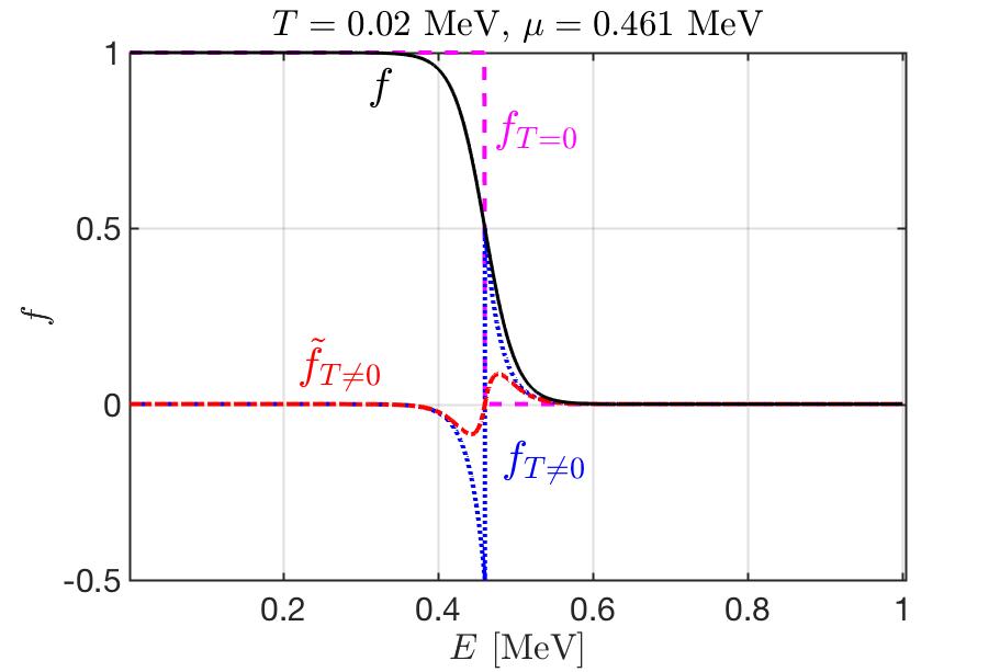
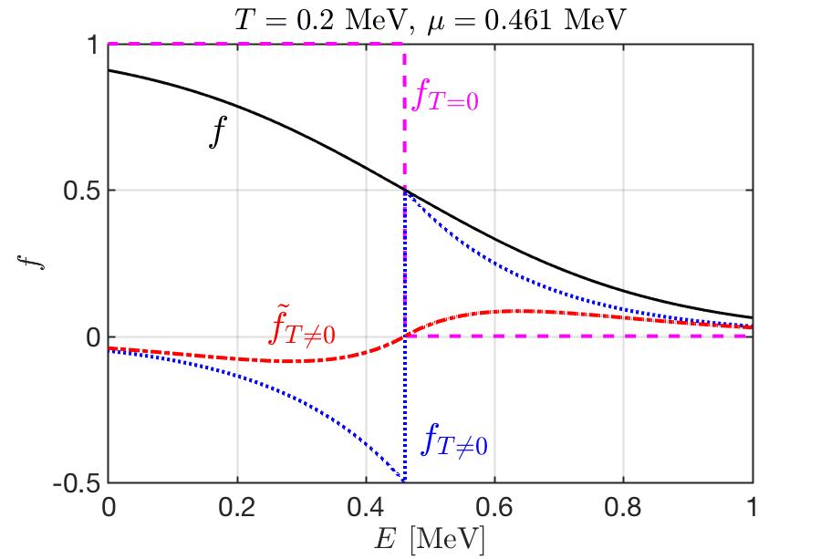
Figure 2: FD distribution (black solid line) as a function of single particle energy for chemical potential $\mu=0.461\text{ MeV}$ on top at a temperature $T=0.02\text{ MeV}$ and on bottom at $T=0.2\text{ MeV}$. The purple dashed line represents the zero temperature component $f_{\mathrm{T}=0}$; blue (dotted) and red (dash-dotted) lines represent the finite temperature components $f_{\mathrm{T\neq 0}}$ and $\widetilde{f}_{\mathrm{T\neq 0}}$ respectively, see Eq. (8).

To illustrate how this novel form of distribution can be used to address the integrals common in statistical physics especially when temperature $T\to 0$, we examine the thermal average of any given function $G(p)$ with smoothness and polynomial growth bounds as $p\to\infty$. The thermal average physical quantity, denoted as $\langle G\rangle_{T}$, is determined by integrating over the D-dimensional phase space

$$\langle G\rangle_{T} \equiv\int^{\infty}_{0}\!\!\frac{d^{D}p}{(2\pi)^{D}}\,G(p)\,f_{FD}(p)=\frac{1}{(2\pi)^{D}}\frac{2\pi^{D/2}}{\Gamma(D/2)}\int^{\infty}_{0}\!\!dp\,p^{D-1}\,G(p)\,f_{FD}(p).$$ (16)

By substituting our novel form of FD distribution, the physical quantity $\langle G\rangle_{T}$ can be expressed as the sum of two distinct components:

$$\langle G\rangle_{T}=\langle G\rangle_{\Theta}+\langle G\rangle_{\Delta T}$$ (17)

where the $\langle G\rangle_{\Theta}$ corresponds to the zero temperature limit and $\langle G\rangle_{\Delta T}$ represents the finite temperature contribution. We have

$$\langle G\rangle_{\Theta}=\frac{1}{(2\pi)^{D}}\frac{2\pi^{D/2}}{\Gamma(D/2)}\int^{\infty}_{0}\!\!dp\,p^{D-1}G(p)\Theta\left(\frac{-E+\mu}{T}\right),\qquad E=\sqrt{p^{2}+m^{2}},$$ (18)

$$\langle G\rangle_{\Delta T}=\frac{1}{(2\pi)^{D}}\frac{2\pi^{D/2}}{\Gamma(D/2)}\int^{\infty}_{0}\!\!dp\,p^{D-1}\,G(p)\,\left[f_{\mathrm{T\neq 0}}(p)+\widetilde{f}_{\mathrm{T\neq 0}}(p)\right].$$ (19)

By employing our FD decomposition, in the following sections we obtain asymptotic expansions of the finite temperature contribution $\langle G\rangle_{\Delta T}$ in different physical regimes of interest. Our novel decomposition guides the asymptotic analysis of $\langle G\rangle_{\Delta T}$ by naturally reorganizing the integrand into a difference of integrals with exponentially decaying integrands. This allows us to utilize asymptotic analysis techniques to extract leading and subleading order behavior as $T\to 0$ and to analytically account for the exact cancellation of certain terms, which otherwise cause problems in numerical computations.

2.2 Traditional Sommerfeld Regime

We now show that the decomposition Eq. (7) naturally motivates certain steps in the derivation of the traditional Sommerfeld expansion, see, e.g., Eq. (58.1) on page 170 of [24], an asymptotic expansion for the difference between a $D$-dimensional thermal average at finite and zero temperature as $T\to 0$ in the regime where $\mu>m$. In this derivation we will be particularly attentive to the location of singularities as well as precisely bounding error terms in the asymptotic expansion. While these details do not play a critical role in obtaining the correct form of the traditional Sommerfeld expansion, they will be important in our new results later in this work and so we wish to review these methods in a more familiar setting first.

Here we will assume that $\mu>m$, $k>1$ is odd, and the density of states $H(E)$ is polynomially bounded on $[m,\infty)$ and is $C^{k}$ on a neighborhood of $\mu$. We will obtain an asymptotic expansion of

$$I\equiv\int_{m}^{\infty}dE\,H(E)f_{FD}(E)$$ (20)

as $T\to 0$. First we note that, starting from $G(p)$ in Eq. (19), the corresponding $H(E)$ is given by

$$H(E)=\frac{1}{(2\pi)^{D}}\frac{2\pi^{D/2}}{\Gamma(D/2)}E(E^{2}-m^{2})^{(D-2)/2}G(\sqrt{E^{2}-m^{2}})$$ (21)

and this $H$ has the required properties if $D\geq 2$ and $G$ is polynomially bounded on $[0,\infty)$ and is $C^{k}$ on a neighborhood of $\sqrt{\mu^{2}-m^{2}}$ (recall that we are assuming $\mu>m$, which allows us to avoid the singularity at $E=m$).

We start by using the decomposition Eq. (7) to break the integral into zero and nonzero temperature contributions

$$I=\int_{m}^{\mu}dE\,H(E)+\int_{m}^{\infty}dE\,H(E)\left[f_{T\neq 0}(E)+\widetilde{f}_{T\neq 0}(E)\right]\,.$$ (22)

Focusing on the non-zero temperature contribution in Eq. (22), we break the second integral into two terms as motivated by the discontinuity of Eq. (8) at $E=\mu$ and then simplify the integrands using Eq. (14) and Eq. (15) as follows:

$$\int_{m}^{\infty}dE\,H(E)\left[f_{T\neq 0}(E)+\widetilde{f}_{T\neq 0}(E)\right]$$ (23)

$$= \int_{\mu}^{\infty}dE\,H(E)\left[f_{T\neq 0}(E)+\widetilde{f}_{T\neq 0}(E)\right]+\int_{m}^{\mu}dE\,H(E)\left[f_{T\neq 0}(E)+\widetilde{f}_{T\neq 0}(E)\right]$$

$$= \int_{\mu}^{\infty}dE\,H(E)\frac{1}{1+e^{(E-\mu)/T}}-\int_{m}^{\mu}dE\,H(E)\frac{1}{1+e^{-(E-\mu)/T}}\,.$$ (24)

The exponentially decaying factors in the above integrands imply that reducing the domains of integration to the intervals $[\mu,\mu+\delta]$ and $[\mu-\delta,\mu]$ respectively for any choice of $\delta>0$ incurs an $\mathcal{O}(e^{-c/T})$ error term for some $c>0$; the assumptions on $H$ imply we can choose $\delta$ so that $H$ is $C^{k}$ on $[\mu-\delta,\mu+\delta]$. To see that the error does in fact have the claimed behavior, use the polynomial boundedness $|H(E)|\leq CE^{q}$ for some $C,q>0$ and change variables to $z=(E-\mu)/T$ to compute

$$\begin{split}&\left|\int_{\mu+\delta}^{\infty}dE\,H(E)\frac{1}{1+e^{(E-\mu)/T}}\right|\\ &\leq C\int_{\mu+\delta}^{\infty}dE\,E^{q}e^{-(E-\mu)/T}=CT\int_{\delta/T}^{\infty}dz\,(Tz+\mu)^{q}e^{-z}\\ &\leq 2^{q}CT\left(T^{q}\int_{\delta/T}^{\infty}dz\,z^{q}e^{-z}+\mu^{q}\int_{\delta/T}^{\infty}dz\,e^{-z}\right)=\mathcal{O}\left(e^{-c/T}\right)\end{split}$$ (25)

for some $c>0$. The second integral in Eq. (24) is handled similarly. The $\mathcal{O}(e^{-c/T})$ error is dominated by $\mathcal{O}(T^{r})$ for any $r$ and so the exact value of $c$ will be seen to be irrelevant for our purposes.

The previous analysis then implies

$$Eq.\,(\ref{eq:traditional_sommerfeld_2_integral})= \int_{\mu}^{\mu+\delta}\!dE\,H(E)\frac{1}{1+e^{(E-\mu)/T}}-\int_{\mu-\delta}^{\mu}\!dE\,H(E)\frac{1}{1+e^{-(E-\mu)/T}}+\mathcal{O}\left(e^{-c/T}\right)\,,$$

$$= T\int_{0}^{\delta/T}dz\,\left[H(\mu+Tz)-H(\mu-Tz)\right]\frac{1}{1+e^{z}}+\mathcal{O}\left(e^{-c/T}\right)\,,$$ (26)

where to obtain the last line we changed variables to $z=(E-\mu)/T$ in the first integral and $z=-(E-\mu)/T$ in the second. The domain of integration is now such that $H$ is $C^{k}$ at $\mu\pm Tz$ for all $z\in[0,\delta/T]$ and therefore we can compute a Taylor expansion up to order $k$ with remainder,

$$H(\mu+Tz)-H(\mu-Tz)=\sum_{n=1,n\text{ odd}}^{k-2}2H^{(n)}(\mu)\frac{(Tz)^{n}}{n!}+R_{k}(z)\,,$$ (27)

$$R_{k}(z)\equiv(Tz)^{k}\int_{0}^{1}ds\,\frac{(1-s)^{k-1}}{(k-1)!}\left[H^{(k)}(\mu+sTz)+H^{(k)}(\mu-sTz)\right]\,,$$ (28)

and $|H^{(k)}(\mu\pm sTz)|\leq C_{k}\equiv\sup_{y\in[\mu-\delta,\mu+\delta]}|H^{(k)}(y)|<\infty$ for all $z\in[0,\delta/T]$, $s\in[0,1]$ (it is finite due to continuity of $H^{(k)}$ on the the compact interval $[\mu-\delta,\mu+\delta]$). Therefore the integral of the remainder term can be bounded as follows

$$\left|T\int_{0}^{\delta/T}R_{k}(z)\frac{1}{1+e^{z}}\right|\leq \frac{2C_{k}}{k!}T^{k+1}\int_{0}^{\delta/T}dz\,z^{k}e^{-z}=\mathcal{O}\left(T^{k+1}\right)\,.$$ (29)

Combining this with Eq. (26) we obtain

$$Eq.\,(\ref{eq:traditional_sommerfeld_2_integral})= \sum_{n=1,n\text{ odd}}^{k-2}2\frac{T^{n+1}}{n!}H^{(n)}(\mu)\int_{0}^{\delta/T}dz\,\frac{z^{n}}{1+e^{z}}+\mathcal{O}\left(T^{k+1}\right)+\mathcal{O}\left(e^{-c/T}\right)\,.$$ (30)

Similarly to the case Eq. (25), the exponential decay factor in the integrand implies that we can change the domains of integration to $[0,\infty)$ at the cost of an $\mathcal{O}(e^{-c/T})$ error term. Using this and then the integral formula

$$\int_{0}^{\infty}\frac{x^{\nu-1}}{e^{x}+1}dx=\begin{cases}\ln(2)\,,&\quad\mathrm{for}\quad\nu=1\\ (1-2^{1-\nu})\Gamma(\nu)\zeta(\nu)\,,&\quad\mathrm{for}\quad\nu>1\end{cases}$$ (31)

(see 3.411.3 on page 353 of [27]) we obtain

$$Eq.\,(\ref{eq:traditional_sommerfeld_2_integral})= \sum_{n=1,n\text{ odd}}^{k-2}2(1-2^{-n})\zeta(n+1)T^{n+1}H^{(n)}(\mu)+\mathcal{O}\left(T^{k+1}\right)\,.$$ (32)

Substituting this into Eq. (20) we obtain the traditional Sommerfeld expansion

$$\int_{m}^{\infty}dE\,H(E)f_{FD}(E)$$

$$= \int_{m}^{\mu}dE\,H(E)+\sum_{n=1,n\text{ odd}}^{k-2}2(1-2^{-n})\zeta(n+1)T^{n+1}H^{(n)}(\mu)+\mathcal{O}(T^{k+1})\,.$$ (33)

We emphasize that the expansion Eq. (33) considers $\mu$ to be fixed and so the implied constant in the $\mathcal{O}(T^{k+1})$ error term has nontrivial $\mu$-dependence. This fact causes the failure of the traditional Sommerfeld expansion in certain cases where one is considering simultaneous $\mu$ and $T$ limits. This is not simply a mathematical consideration, as simultaneous limits are required to maintain appropriate physical parameters as $T\to 0$, e.g., the moderate density regime shown in Figure 1. In the remainder of this work we derive several novel asymptotic expansions of FD integrals by precisely considering different $\mu$, $T$ limits. The expansions in Sections 2.3 and 2.4 can still be considered to be of Sommerfeld type, while the regime considered in Section 3 leads to a wholly novel expansion.

2.3 Sommerfeld Expansion in the Nonrelativistic Degenerate Fermi Gas Regime $T\ll\mu-m\ll m$

In this section we use the decomposition Eq. (7) to further investigate the Sommerfeld expansion in the limit where $T\ll\mu-m\ll m$. While in essence the traditional Sommerfeld expansion applies to this regime, a naive use of Eq. (33) often results in one encountering numerical difficulties due to singular behavior of various coefficients in the limit $\mu\to m$. In this section we derive a formula that precisely accounts for these singularities; this formula makes it straightforward to compute the coefficients in the expansion up to any desired order via a computer algebra system.

More specifically, in this section we will assume $D\geq 2$ and

$$\mu=m+\Delta\mu\,,\,\Delta\mu>0\,\,\text{ and }\,\,\widetilde{T}=d\Delta\widetilde{\mu}^{1+\gamma}\,,\,\,d,\gamma>0\,,$$ (34)

where $\widetilde{T}\equiv T/m$ and $\Delta\widetilde{\mu}\equiv\Delta\mu/m$; these scalings imply that $T\ll\mu-m\ll m$ as $\Delta\widetilde{\mu}\to 0$, matching the stated goal here. We let $G(p)$, $p\in[0,\infty)$, be a $C^{k}$ function whose zeroth through $k$’th derivatives are polynomially bounded and will study $\langle G\rangle_{\Delta T}$ in the limit $\Delta\widetilde{\mu}\to 0^{+}$. The final result is found in Theorem 2 below. To proceed with the derivation, first change variables in Eq. (19) to $E=\sqrt{p^{2}+m^{2}}$ and then use Eq. (14) and Eq. (15):

$$\int_{0}^{\infty}dp\,p^{D-1}G(p)(f_{T\neq 0}+\widetilde{f}_{T\neq 0})$$

$$= \int_{m}^{\infty}dE\,E(E^{2}-m^{2})^{(D-2)/2}G\left(\sqrt{E^{2}-m^{2}}\right)(f_{T\neq 0}+\widetilde{f}_{T\neq 0})$$

$$= \int_{\mu}^{\infty}dE\,E(E^{2}-m^{2})^{(D-2)/2}G\left(\sqrt{E^{2}-m^{2}}\right)\frac{1}{1+e^{(E-\mu)/T}}$$ (35)

$$-\int_{m}^{\mu}dE\,E(E^{2}-m^{2})^{(D-2)/2}G\left(\sqrt{E^{2}-m^{2}}\right)\frac{1}{1+e^{(\mu-E)/T}}\,.$$

Next consider the first integral in Eq. (35). In general, its integrand will have a singularity at $E=m$. As the lower limit of integration approaches $m$ in the regime under consideration, it is necessary to carefully resolve that singularity. We have chosen to begin with the integral expressed in terms of $p$ because it simplifies this analysis, due to $E=\sqrt{p^{2}+m^{2}}$ being is a smooth function of $p$ but not vice versa. Thus if one begins with a smooth density of states $H(E)$, the corresponding $G(p)$ will also be smooth but the reverse is not true. We note that if one is interested in $G(p)$ that is not smooth at $p=0$ then the following derivation can be easily modified to account for a power-law singularity of $G$ at $0$.

To derive an expansion that correctly handles the singular behavior of the integrands in Eq. (35) at $E=m$, we first change variables to $z=(E-m)/m$ to obtain

$$\int_{\mu}^{\infty}dE\,E(E^{2}-m^{2})^{(D-2)/2}G\left(\sqrt{E^{2}-m^{2}}\right)\frac{1}{1+e^{(E-\mu)/T}}$$

$$= m^{D}\int_{\Delta\widetilde{\mu}}^{\infty}dz\,(z+1)[(z+1)^{2}-1]^{(D-2)/2}G\left(m\sqrt{(z+1)^{2}-1}\right)\frac{1}{1+e^{(z-\Delta\widetilde{\mu})/\widetilde{T}}}$$

$$= m^{D}\int_{\Delta\widetilde{\mu}}^{\infty}dz\,(z+1)(z+2)^{(D-2)/2}G\left(m\sqrt{z}\sqrt{z+2}\right)\frac{z^{(D-2)/2}}{1+e^{(z-\Delta\widetilde{\mu})/\widetilde{T}}}\,.$$ (36)

We have separated out the (possible) singularity coming from $z^{(D-2)/2}$ but there still remains a potential singularity at $z=0$ coming from the argument of $G$. The term involving $G$ does not always have a Taylor expansion, but it does have a more general asymptotic expansion which we can obtain as follows. Define

$$F(y,m)\equiv(y^{2}+1)(y^{2}+2)^{(D-2)/2}G\left(my\sqrt{y^{2}+2}\right)\,.$$ (37)

We have assumed that $G$ is $C^{k}$ on $[0,\infty)$ with polynomially bounded zeroth through $k$’th derivatives and therefore $y\mapsto F(y,m)$ also has these properties. Hence we can use Taylor’s theorem with remainder to write

$$F(y,m)= \sum_{n=0}^{k-1}a_{n}(m)y^{n}+R_{k}(y,m)\,,\,\,\,a_{n}(m)=\frac{1}{n!}\partial_{y}^{n}F(0,m)\,,$$ (38)

where the remainder term is given by

$$R_{k}(y,m)=y^{k}\int_{0}^{1}\frac{(1-s)^{k-1}}{(k-1)!}\partial_{y}^{k}F(sy,m)ds$$ (39)

and can be bounded via

$$|R_{k}(y,m)|\leq y^{k}[\alpha_{k}(m)+\beta_{k}(m)y^{q_{k}}]$$ (40)

for some coefficients $\alpha_{k},\beta_{k}\geq 0$ and power $q_{k}\geq 0$ due to the polynomial boundedness of $\partial_{y}^{k}F$.

With this we have

$$Eq.\,(\ref{eq:T_faster_int_1_change_vars})= m^{D}\!\int_{\Delta\widetilde{\mu}}^{\infty}\!dz\,F(\sqrt{z},m)\frac{z^{(D-2)/2}}{1+e^{(z-\Delta\widetilde{\mu})/\widetilde{T}}}$$ (41)

$$= \sum_{n=0}^{k-1}a_{n}(m)m^{D}\!\!\int_{\Delta\widetilde{\mu}}^{\infty}\!dz\,\frac{z^{(n+D-2)/2}}{1+e^{(z-\Delta\widetilde{\mu})/\widetilde{T}}}+m^{D}\!\!\int_{\Delta\widetilde{\mu}}^{\infty}\!dz\,R_{k}(\sqrt{z},m)\frac{z^{(D-2)/2}}{1+e^{(z-\Delta\widetilde{\mu})/\widetilde{T}}}\,.$$

The integral of the remainder term can be bounded by using Eq. (40) as follows

$$\left|m^{D}\int_{\Delta\widetilde{\mu}}^{\infty}dz\,R_{k}(\sqrt{z},m)\frac{z^{(D-2)/2}}{1+e^{(z-\Delta\widetilde{\mu})/\widetilde{T}}}\right|$$ (42)

$$\leq m^{D}\int_{\Delta\widetilde{\mu}}^{\infty}dz\,z^{k/2}[\alpha_{k}(m)+\beta_{k}(m)z^{q_{k}/2}]z^{(D-2)/2}e^{-(z-\Delta\widetilde{\mu})/\widetilde{T}}$$

$$= d\alpha_{k}(m)m^{D}\Delta\widetilde{\mu}^{(k+D)/2+\gamma}\int_{0}^{\infty}dx\,(1+d\Delta\widetilde{\mu}^{\gamma}x)^{(k+D-2)/2}e^{-x}$$

$$+d\beta_{k}(m)m^{D}\Delta\widetilde{\mu}^{(k+q_{k}+D)/2+\gamma}\int_{0}^{\infty}dx\,(1+d\Delta\widetilde{\mu}^{\gamma}x)^{(k+q_{k}+D-2)/2}e^{-x}$$

$$= \mathcal{O}\left(\Delta\widetilde{\mu}^{(k+D)/2+\gamma}\right)\quad\text{as}\quad\Delta\widetilde{\mu}\to 0^{+}\,,$$ (43)

where we changed variables to $x=(z-\Delta\widetilde{\mu})/\widetilde{T}$ and used Eq. (34). Making this same change of variables in the remaining terms, we therefore obtain

$$Eq.\,(\ref{eq:T_faster_int_1_change_vars})= \sum_{n=0}^{k-1}da_{n}(m)m^{D}\Delta\widetilde{\mu}^{(n+D)/2+\gamma}\!\int_{0}^{\infty}\!dx\,\frac{(1+d\Delta\widetilde{\mu}^{\gamma}x)^{(n+D-2)/2}}{1+e^{x}}$$ (44)

$$+\mathcal{O}\left(\Delta\widetilde{\mu}^{(k+D)/2+\gamma}\right)\,.$$

These remaining integrals are smooth as functions of $d\Delta\widetilde{\mu}^{\gamma}$ and can be Taylor expanded to order $k-1$ by differentiating under the integral, with remainder $\mathcal{R}_{k}(C,x)$:

$$\int_{0}^{\infty}dx\,\frac{(1+Cx)^{\nu}}{1+e^{x}}=\int_{0}^{\infty}dx\left(\sum_{j=0}^{k-1}\frac{1}{j!}\left.\frac{\partial^{j}}{\partial C^{j}}\right|_{C=0}\!\!\!\frac{(1+Cx)^{\nu}}{1+e^{x}}C^{j}+\mathcal{R}_{k}(C,x)\right)$$ (45)

$$= \sum_{j=0}^{k-1}\frac{1}{j!}\left(\prod_{\ell=0}^{j-1}(\nu-\ell)\right)C^{j}\int_{0}^{\infty}dx\frac{x^{j}}{1+e^{x}}$$

$$+C^{k}\int_{0}^{\infty}dx\frac{x^{k}}{1+e^{x}}\int_{0}^{1}ds\frac{(1-s)^{k-1}}{(k-1)!}\left(\prod_{\ell=0}^{k-1}(\nu-\ell)\right)(1+sCx)^{\nu-k}$$

$$= \ln(2)+\sum_{j=1}^{k-1}\frac{1}{j!}\left(\prod_{\ell=0}^{j-1}(\nu-\ell)\right)C^{j}(1-2^{-j})\Gamma(j+1)\zeta(j+1)+\mathcal{O}(C^{k})\,,$$

where we used the integral formula Eq. (31). Now we apply this to the terms in Eq. (44) with $C=d\Delta\widetilde{\mu}^{\gamma}$ and $\nu=(n+D-2)/2$; note that for each $n$ we must expand Eq. (45) up to order $k_{n}\equiv\lceil(k-n)/(2\gamma)\rceil$ so that the the remainder term in Eq. (45) is of the same or higher order than the remainder in Eq. (43) for each $n$. Doing this yields

$$Eq.\,(\ref{eq:T_faster_int_1_change_vars})= \sum_{n=0}^{k-1}da_{n}(m)m^{D}\Delta\widetilde{\mu}^{(n+D)/2+\gamma}\bigg{[}\ln(2)$$ (46)

$$+\sum_{j=1}^{k_{n}-1}d^{j}\Delta\widetilde{\mu}^{j\gamma}\left(\prod_{\ell=0}^{j-1}[(n+D-2)/2-\ell]\right)(1-2^{-j})\zeta(j+1)\bigg{]}$$

$$+\mathcal{O}\left(\Delta\widetilde{\mu}^{(k+D)/2+\gamma}\right)\,.$$

This completes the asymptotic expansion of the first integral in Eq. (35).

Now consider the second integral in Eq. (35). Again we change variables to $z=(E-m)/m$ and make use of Eq. (37) and Eq. (38):

$$\int_{m}^{\mu}dE\,E(E^{2}-m^{2})^{(D-2)/2}G\left(\sqrt{E^{2}-m^{2}}\right)\frac{1}{1+e^{(\mu-E)/T}}$$ (47)

$$= m^{D}\int_{0}^{\Delta\widetilde{\mu}}dz\,F(\sqrt{z},m)\frac{z^{(D-2)/2}}{1+e^{(\Delta\widetilde{\mu}-z)/\widetilde{T}}}$$

$$= \sum_{n=0}^{k-1}a_{n}(m)m^{D}\int_{0}^{\Delta\widetilde{\mu}}dz\,\frac{z^{(n+D-2)/2}}{1+e^{(\Delta\widetilde{\mu}-z)/\widetilde{T}}}+m^{D}\int_{0}^{\Delta\widetilde{\mu}}dz\,R_{k}(\sqrt{z},m)\frac{z^{(D-2)/2}}{1+e^{(\Delta\widetilde{\mu}-z)/\widetilde{T}}}\,.$$

We bound the integral of the remainder by again using Eq. (40)

$$\left|m^{D}\int_{0}^{\Delta\widetilde{\mu}}dz\,R_{k}(\sqrt{z},m)\frac{z^{(D-2)/2}}{1+e^{(\Delta\widetilde{\mu}-z)/\widetilde{T}}}\right|$$ (48)

$$\leq m^{D}\int_{0}^{\Delta\widetilde{\mu}}dz\,\left[\alpha_{k}(m)+\beta_{k}(m)z^{q_{k}/2}\right]z^{(k+D-2)/2}e^{-(\Delta\widetilde{\mu}-z)/\widetilde{T}}$$

$$\leq m^{D}\widetilde{T}\left[\alpha_{k}(m)\Delta\widetilde{\mu}^{(k+D-2)/2}+\beta_{k}(m)\Delta\widetilde{\mu}^{(k+q_{k}+D-2)/2}\right]$$

$$= \mathcal{O}\left(\Delta\widetilde{\mu}^{(k+D)/2+\gamma}\right)\,.$$

Therefore

$$Eq.\,(\ref{eq:T_faster_int_2_change_vars})= \sum_{n=0}^{k-1}da_{n}(m)m^{D}\Delta\widetilde{\mu}^{(n+D)/2+\gamma}\int^{\Delta\widetilde{\mu}/\widetilde{T}}_{0}du\,\frac{(1-\widetilde{T}u/\Delta\widetilde{\mu})^{(n+D-2)/2}}{1+e^{u}}$$ (49)

$$+\mathcal{O}(\Delta\widetilde{\mu}^{(k+D)/2+\gamma})\,,$$

where we changed variables to $u=(\Delta\widetilde{\mu}-z)/\widetilde{T}$. The remaining integrals can be expanded using the following computation for $C>0$:

$$\int_{0}^{1/C}du\,\frac{(1-Cu)^{\nu}}{1+e^{u}}=\int_{0}^{1/C}du\left(\sum_{j=0}^{k-1}\frac{1}{j!}\left.\frac{\partial^{j}}{\partial C^{j}}\right|_{C=0}!\!\!\frac{(1-Cu)^{\nu}}{1+e^{u}}C^{j}+\mathcal{R}_{k}(C,u)\right)$$ (50)

$$= \sum_{j=0}^{k-1}\frac{C^{j}}{j!}(-1)^{j}\left(\prod_{\ell=0}^{j-1}(\nu-\ell)\right)\int_{0}^{1/C}du\,\frac{u^{j}}{1+e^{u}}$$

$$+C^{k}(-1)^{k}\left(\prod_{\ell=0}^{k-1}(\nu-\ell)\right)\int_{0}^{1/C}du\frac{1}{1+e^{u}}u^{k}\int_{0}^{1}ds\,\frac{(1-s)^{k-1}}{(k-1)!}(1-Csu)^{\nu-k}\,.$$

When $\nu\geq k$ we have $(1-Csu)^{\nu-k}\leq 1$ and so it is straightforward to see that the integral of the remainder $\mathcal{R}_{k}(C,u)$ is $\mathcal{O}(C^{k})$ as $C\to 0$. When $\nu<k$ we have $(1-Csu)^{\nu-k}\leq(1-s)^{\nu-k}$ and so the remainder can be bounded as follows

$$\left|C^{k}(-1)^{k}\left(\prod_{\ell=0}^{k-1}(\nu-\ell)\right)\int_{0}^{1/C}du\frac{1}{1+e^{u}}u^{k}\int_{0}^{1}ds\,\frac{(1-s)^{k-1}}{(k-1)!}(1-Csu)^{\nu-k}\right|$$

$$\leq C^{k}\left|\left(\prod_{\ell=0}^{k-1}(\nu-\ell)\right)\right|\int_{0}^{1/C}du\frac{1}{1+e^{u}}u^{k}\int_{0}^{1}ds\,\frac{(1-s)^{\nu-1}}{(k-1)!}=\mathcal{O}(C^{k})$$ (51)

for all $\nu>0$. Therefore we have shown

$$\int_{0}^{1/C}du\,\frac{(1-Cu)^{\nu}}{1+e^{u}}=\sum_{j=0}^{k-1}\frac{C^{j}}{j!}(-1)^{j}\left(\prod_{\ell=0}^{j-1}(\nu-\ell)\right)\int_{0}^{1/C}du\,\frac{u^{j}}{1+e^{u}}+\mathcal{O}(C^{k})$$ (52)

(note that this trivially holds for $\nu=0$ as well). Also note that the exponential decay of the integrand implies

$$\int_{1/C}^{\infty}du\,\frac{u^{j}}{1+e^{u}}=\mathcal{O}(C^{k})$$ (53)

for any $k$ and hence we are free to change the upper limits of integration to $\infty$ without changing the order of the error, thereby yielding:

$$\int_{0}^{1/C}du\,\frac{(1-Cu)^{\nu}}{1+e^{u}}=\sum_{j=0}^{k-1}\frac{C^{j}}{j!}(-1)^{j}\left(\prod_{\ell=0}^{j-1}(\nu-\ell)\right)\int_{0}^{\infty}du\,\frac{u^{j}}{1+e^{u}}+\mathcal{O}(C^{k})\,.$$ (54)

For each $n$ we use this expansion up to order $k_{n}=\lceil(k-n)/(2\gamma)\rceil$ with $C\equiv\widetilde{T}/\Delta\widetilde{\mu}=d\Delta\widetilde{\mu}^{\gamma}$ and $\nu=(n+D-2)/2$ with $n\geq 0$, $D\geq 2$, along with the integral formulas Eq. (31). Substituting these into Eq. (49) gives

$$Eq.\,(\ref{eq:T_faster_int_2_change_vars})= \sum_{n=0}^{k-1}da_{n}(m)m^{D}\Delta\widetilde{\mu}^{(n+D)/2+\gamma}\bigg{[}\ln(2)$$ (55)

$$+\sum_{j=1}^{k_{n}-1}(-1)^{j}d^{j}\Delta\widetilde{\mu}^{j\gamma}\left(\prod_{\ell=0}^{j-1}[(n+D-2)/2-\ell]\right)(1-2^{-j})\zeta(j+1)\bigg{]}$$

$$+\mathcal{O}\left(\Delta\widetilde{\mu}^{(k+D)/2+\gamma}\right)\,,$$

This completes the asymptotic expansion of the second integral in Eq. (35).

Finally, subtracting Eq. (55) from Eq. (46) and canceling the shared terms (in particular, they cancel at leading order) we obtain the following asymptotic expansion.

Theorem 2.

Let $D\geq 2$, $\mu=m+\Delta\mu$, $\Delta\mu>0$ and $\widetilde{T}=d\Delta\widetilde{\mu}^{1+\gamma}$$d,\gamma>0$. Let $k\in\mathbb{Z}^{+}$ and suppose $G(p)$ is a $C^{k}$ function on $p\in[0,\infty)$ whose zeroth through $k$’th derivatives are polynomially bounded. Then

$$\int_{0}^{\infty}dp\,p^{D-1}G(p)(f_{T\neq 0}+\widetilde{f}_{T\neq 0})$$ (56)

$$= \sum_{n=0}^{k-1}da_{n}(m)m^{D}\Delta\widetilde{\mu}^{(n+D)/2+\gamma}$$ (57)

$$\times\sum_{j=1,\mathrm{odd}}^{\lceil(k-n)/(2\gamma)\rceil-1}2d^{j}\Delta\widetilde{\mu}^{j\gamma}\left(\prod_{\ell=0}^{j-1}[(n+D-2)/2-\ell]\right)(1-2^{-j})\zeta(j+1)$$

$$+\mathcal{O}\left(\Delta\widetilde{\mu}^{(k+D)/2+\gamma}\right)$$

as $\Delta\widetilde{\mu}\to 0^{+}$, where $\Delta\widetilde{\mu}=(\mu-m)/m$, $\widetilde{T}=T/m$, and

$$a_{n}(m)=\frac{1}{n!}\partial_{y}^{n}|_{y=0}\left[(y^{2}+1)(y^{2}+2)^{(D-2)/2}G\left(my\sqrt{y^{2}+2}\right)\right]\,.$$ (58)

We provide explicit formulas for the first few $a_{n}$’s below:

$$a_{0}(m)=2^{(D-2)/2}G(0)\,,$$ (59)

$$a_{1}(m)=2^{(D-1)/2}mG^{\prime}(0)\,,$$

$$a_{2}(m)=2^{(D-6)/2}\left[(D+2)G(0)+4m^{2}G^{\prime\prime}(0)\right]\,,$$

$$a_{3}(m)=2^{(D-5)/2}\left((D+3)mG^{\prime}(0)+\frac{4}{3}m^{3}G^{\prime\prime\prime}(0)\right)\,,$$

where the primes denote derivatives of $G(p)$ with respect to $p$. In dimension $D=3$ the leading order term in Eq. (57) will be determined by the first $n$ for which $a_{n}(m)\neq 0$, which results in a term that scales with $\Delta\widetilde{\mu}^{(n+3)/2+2\gamma}$. In Figure 3 we show a comparison between the expansion Eq. (57) and numerical integration of Eq. (56), demonstrating the effectiveness of the expansion as well as error scaling that matches the result Eq. (57).

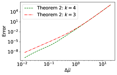
Figure 3: Comparison of the computation of $\langle G\rangle_{\Delta T}$ (left) using the expansion Eq. (57) for $\gamma=1/2$, $d=1$, and $G(p)=E$, with the result obtained via numerical integration of Eq. (56). The right plot shows the difference between the numerical result and the expansion Eq. (57) corresponding to $k=3$ and $k=4$. The right plot shows the difference between the numerical result and the two expansions. On a log-log plot the slopes of the error can be measured to be approximately $4$ (for $k=4$) and $7/2$ (for $k=3$), correctly matching the order of the expansion error in $\Delta\widetilde{\mu}$ as stated in Eq. (57).

2.4 Sommerfeld Expansion in the Relativistic, Dense Regime $\mu\gg T\gg m$

Interestingly, there is also a high temperature regime ($\mu\gg T\gg m$) where the traditional Sommerfeld expansion provides a good approximation to thermal averages.

Theorem 3 (High-Temperature Sommerfeld Expansion).

Let $k\in\mathbb{Z}^{+}$ be odd and suppose that $H(E)$ is continuous on $[m,\infty)$, is smooth on a neighborhood of $\infty$, and

$$H^{(k)}(E)=a_{k}E^{q_{k}}+\mathcal{O}(E^{q_{k}-1})$$ (60)

as $E\to\infty$ for some $a_{k}\neq 0$, $q_{k}\in\mathbb{R}$. Let $\mu=m[1+B(T/m)^{1+\gamma}]$, $\gamma,B>0$. Then

$$\int_{m}^{\infty}dE\,H(E)f_{FD}(E)$$

$$= \int_{m}^{\mu}dE\,H(E)+\sum_{n=1,n\text{ odd}}^{k-2}2(1-2^{-n})\zeta(n+1)T^{n+1}H^{(n)}(\mu)+\mathcal{O}(\mu^{q_{k}}T^{k+1})$$ (61)

as $T\to\infty$.

To prove Eq. (61), parameterize $\mu$ as a function of $T$ as follows

$$\mu=m[1+B(T/m)^{1+\gamma}]\,,\,\,\gamma,B>0\,.$$ (62)

and assume that the density of states $H(E)$ has the properties stated in Theorem 3. By integrating Eq. (60) and combining it with the assumption that $H$ is continuous we can conclude that $H$ is also polynomially bounded on $[m,\infty)$. We note that, by definition, the asymptotic behavior Eq. (60) implies that there exists $E_{0}$ and $C$ such that $H$ is smooth on $[E_{0},\infty)$ and $|H^{(k)}(E)-a_{k}E^{q_{k}}|\leq CE^{q_{k}-1}$ for all $E\in[E_{0},\infty)$. For the remainder of this derivation we assume that $T$ is large enough to ensure $\mu\geq E_{0}$.

Now consider the nonzero temperature component of the decomposition Eq. (7) and use Eq. (14) and Eq. (15) to write

$$\int_{m}^{\infty}dE\,H(E)(f_{T\neq 0}+\widetilde{f}_{T\neq 0})$$

$$= \int_{\mu}^{\infty}dE\,H(E)\frac{1}{1+e^{(E-\mu)/T}}-\int_{m}^{\mu}dE\,H(E)\frac{1}{1+e^{(\mu-E)/T}}$$

$$= T\int_{0}^{\infty}dz\,H(\mu+Tz)\frac{1}{1+e^{z}}-T\int^{(\mu-m)/T}_{0}dz\,H(\mu-Tz)\frac{1}{1+e^{z}}\,,$$ (63)

where we changed variables to $z=(E-\mu)/T$ in the first integral and $z=(\mu-E)/T$ in the second. Due to the exponentially decaying factors in the integrands in Eq. (63) along with polynomial boundedness of $H$, we can shrink the upper limits of integration to $(\mu-E_{0})/T$, thereby ensuring that $\mu-Tz\geq E_{0}$ on the domain of integration, with the error incurred by this change being $\mathcal{O}(T^{-r})$ as $T\to\infty$ for any choice of $r>0$. A similar bound was derived in the traditional Sommerfeld case, see Section 2.2 for details, though here this error term also accounts for the dependence on $\mu$ in accordance with Eq. (62). As we will see, the $\mathcal{O}(T^{-r})$ error term will be negligible compared to the other asymptotic approximations made below. In light of this we can write

$$\int_{m}^{\infty}dE\,H(E)(f_{T\neq 0}+\widetilde{f}_{T\neq 0})$$

$$= T\int_{0}^{\frac{\mu-E_{0}}{T}}dz\,\frac{H(\mu+Tz)-H(\mu-Tz)}{1+e^{z}}+\mathcal{O}(T^{-r})\,.$$ (64)

As $\mu\pm Tz\geq E_{0}$ for all $z$ in the domain of integration, we can compute a Taylor expansion with remainder up to order $k$ on this domain as follows:

$$H(\mu+Tz)-H(\mu-Tz)=\sum_{n=1,n\text{ odd}}^{k-2}2H^{(n)}(\mu)\frac{(Tz)^{n}}{n!}$$ (65)

$$\qquad\qquad\qquad+(Tz)^{k}\int_{0}^{1}ds\,\frac{(1-s)^{k-1}}{(k-1)!}\left[H^{(k)}(\mu+sTz)+H^{(k)}(\mu-sTz)\right]\,.$$

We emphasize that the reason for restricting the domain of integration in Eq. (64) (with the difference being accounted for in the error term) is that we are only assuming $H$ is $C^{k}$ on a neighborhood of $\infty$, and so the Taylor expansion argument is only valid on the restricted domain.

Substituting Eq. (65) this into Eq. (64) we can compute

$$\int_{m}^{\infty}dE\,H(E)(f_{T\neq 0}+\widetilde{f}_{T\neq 0})$$

$$= \sum_{n=1,n\text{ odd}}^{k-2}\frac{2T^{n+1}}{n!}H^{(n)}(\mu)\int_{0}^{\frac{\mu-E_{0}}{T}}dz\,\frac{z^{n}}{1+e^{z}}+R_{k}+\mathcal{O}(T^{-r})$$

$$= \sum_{n=1,n\text{ odd}}^{k-2}2(1-2^{-n})\zeta(n+1)T^{n+1}H^{(n)}(\mu)+R_{k}+\mathcal{O}(T^{-r})\,,$$ (66)

where to obtain the last line we again made use of the freedom to change the limits of integration while only incurring $\mathcal{O}(T^{-r})$ error and then used the integral formula Eq. (31). The integrated remainder term is given by

$$R_{k}\equiv T^{k+1}\int_{0}^{\frac{\mu-E_{0}}{T}}dz\,\frac{z^{k}}{1+e^{z}}\int_{0}^{1}ds\,\frac{(1-s)^{k-1}}{(k-1)!}\left[H^{(k)}(\mu+sTz)+H^{(k)}(\mu-sTz)\right]\,.$$ (67)

Eq. (60) implies that $|H^{(k)}(E)|\leq CE^{q_{k}}$ on $[E_{0},\infty)$ for some $C>0$. Using this we can bound the integral of the remainder as follows:

$$|R_{k}|\leq CT^{k+1}\int_{0}^{\frac{\mu-E_{0}}{T}}dz\,\frac{z^{k}}{1+e^{z}}\int_{0}^{1}ds\,\frac{(1-s)^{k-1}}{(k-1)!}\left(|\mu+sTz|^{q_{z}}+|\mu-sTz|^{q_{k}}\right)$$

$$\leq 2^{q_{k}+1}CT^{k+1}\int_{0}^{\infty}dz\,\frac{z^{k}}{1+e^{z}}\int_{0}^{1}ds\,\frac{(1-s)^{k-1}}{(k-1)!}\left[\mu^{q_{k}}+(sTz)^{q_{k}}\right]$$

$$= \mathcal{O}(\mu^{q_{k}}T^{k+1})$$ (68)

as $T\to\infty$. Note that due to the relation Eq. (62) between $\mu$ and $T$ we can equivalently write the error term as $\mathcal{O}(T^{(1+\gamma)q_{k}+k+1})$ and so the $\mathcal{O}(T^{-r})$ error term is negligible in comparison. Combining the bound Eq. (68) with Eq. (66) we obtain

$$\int_{m}^{\infty}dE\,H(E)f_{FD}(E)$$

$$= \int_{m}^{\mu}dE\,H(E)+\sum_{n=1,n\text{ odd}}^{k-2}2(1-2^{-n})\zeta(n+1)T^{n+1}H^{(n)}(\mu)+\mathcal{O}(\mu^{q_{k}}T^{k+1})$$ (69)

as $T\to\infty$. This completes the proof of Theorem 3.

Unless $q_{k}$ is sufficiently negative, the absolute error in Eq. (61) grows as $T\to\infty$, however the relative error decays as we now show. First assume $q_{k}>0$ and integrate Eq. (60) twice at the Fermi energy $E=\mu$ to get

$$H^{(k-2)}(\mu)=\frac{a_{k}}{(q_{k}+1)(q_{k}+2)}\mu^{q_{k}+2}+\mathcal{O}(\mu^{q_{k}+1})$$ (70)

as $\mu\to\infty$. Therefore, the ratio of the error to the last included term in the expansion behaves as

$$\frac{\mathcal{O}(\mu^{q_{k}}T^{k+1})}{T^{k-1}H^{(k-2)}(\mu)}=\frac{T^{2}}{\mu^{2}}\frac{\mathcal{O}(1)}{\frac{a_{k}}{(q_{k}+1)(q_{k}+2)}+\mathcal{O}(\mu^{-1})}=\mathcal{O}(T^{-2\gamma})\,,$$ (71)

which approaches $0$ as $T\to\infty$. To obtain Eq. (71) we used Eq. (62) and also that $a_{k}\neq 0$. Continuing to integrate Eq. (70), one sees that earlier terms in the sum dominate the error term to a greater degree. Therefore the expansion Eq. (69) properly captures leading and sub-leading behavior, with a subdominant error term and a decaying relative error when $q_{k}>0$. When $q_{k}\leq 0$, integrating Eq. (60) becomes more subtle due to the need to handle potential logarithm and constant terms that arise. However, if instead we make the additional assumptions

$$H^{(k-j)}(E)=a_{k-j}E^{q_{k}+j}+\mathcal{O}(E^{q_{k}+j-1})$$ (72)

for $j=2,...,k-1$ with $a_{k-j}\neq 0$ then a similar computation to Eq. (71) shows

$$\frac{\mathcal{O}(\mu^{q_{k}}T^{k+1})}{T^{n+1}H^{(n)}(\mu)}=\mathcal{O}(T^{-(k-n)\gamma})$$ (73)

for all $n=1,...,k-2$ and therefore the error term in Eq. (69) is again seen to be dominated by all other terms in the summation as $T\to\infty$.

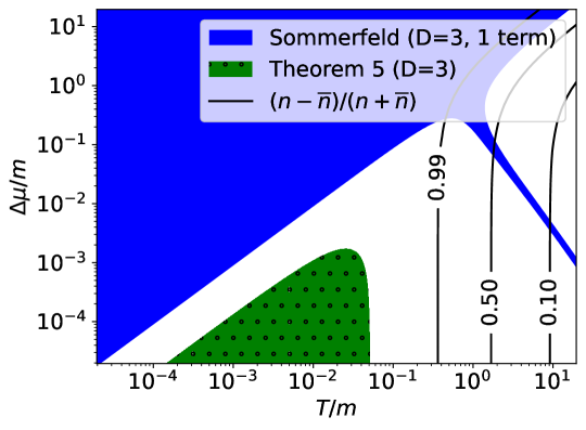
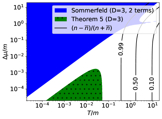
Figure 4: Comparison of domains of validity for $D=3$ in $(T/m,\Delta\mu/m)$-space ($\Delta\mu\equiv\mu-m$), including relativistic parameter range, considering in top frame one asymptotic and in bottom frame two asymptotic terms; we show the Sommerfeld expansion (solid blue), and the expansion from Theorem 5 (dotted green). Validity is defined as the computation of $\langle G\rangle_{T}$ having relative error less that $10\%$ for the choice $G(p)=1$. See text for further details.

In Figure 4 we demonstrate numerically that the Sommerfeld expansion from Theorem 3 applies to the high-temperature region, in addition to the well-known low temperature regime. In contrast, our new expansion, see below Theorem 5, applies when $|\Delta\mu|\ll T\ll m$, a regime not covered by either the Sommerfeld expansion or Boltzmann approximation; for a comparison with the latter see Figure 1. The domians of validity of both expansions predominantly lie in the particle dominated region where $n\gg\overline{n}$ ($n$ and $\overline{n}$ denote number of particles and antiparticles respectively); see the solid black contours. The pair dominated region ($\overline{n}\approx n$) on the right side of the domain requires other methods. We note that the domain of validity when using 2 terms (bottom frame Figure 4) of the Sommerfeld expansion is reduced in many areas, as compared to the region for 1 term (top frame). This is typical of results such as Theorem 3 that give asymptotic, but not convergent, expansions; adding additional terms does not necessarily increase the accuracy at fixed values of the parameters $\mu$ and $T$. The leg structure of the blue domain arises since the approximate and exact results cross, thus this reflects only an accidental exact agreement between the numerical and one-term asymptotic results.

3 Non-Sommerfeld Few Particle Regime

3.1 Asymptotic Expansion in the Regime $T\to 0$ with $\mu-m\ll T$

In this section we study thermal averages when $\mu-m\ll T\ll m$, a regime where we demonstrate a complete failure of the Sommerfeld formula. The techniques we use to study this regime are similar to those employed in Section 2.3, but this time they lead to a wholly distinct and novel asymptotic expansion. In Figure 5 we preview this new result, which is stated in Theorem 5 below. In this figure we have parameterized $\mu-m=\mathcal{O}(T^{3/2})$ and so $\mu-m$ approaches zero faster than $T$. Note that here the Sommerfeld expansion Eq. (33) (red dot-dashed lines) fails at low temperature while our Theorem 5 (green dashed lines) provides an accurate approximation. One can see from the figure that the traditional Sommerfeld expansion is in fact a high temperature approximation under this relation between $\mu$ and $T$; this corresponds to the behavior proven in Theorem 3 above.

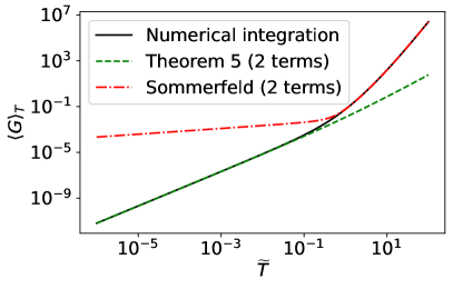
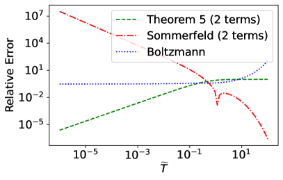
Figure 5: Left: Comparison of asymptotic expansions of $\langle G\rangle_{T}$, $G(p)=1$, via the Sommerfeld expansion Eq. (33) (red dot-dashed line) and the new expansion Eq. (89) (green dashed line) where $\mu=m(1+\widetilde{T}^{3/2})$. Under this relationship between $\mu$ and $T$, Theorem 3 and Theorem 5 respectively prove that Eq. (61) is valid at high temperature and Eq. (89) is valid at low temperature; we see this reflected in the figure. Right: The relative error of these asymptotic expansions, also compared with that of the Boltzmann approximation.

We now proceed with a detailed derivation of the new expansion. To make our assumptions explicit, here we consider a $D$-dimensional thermal average ($D\geq 2$) of a function $G(p)$, $p\in[0,\infty)$ that is $C^{k}$ and whose zeroth through $k$’th derivatives are polynomially bounded, and will assume that $\mu=m+bT$, $b\in\mathbb{R}$. To begin the derivation, first change variables in Eq. (16) to $z=(E-m)/m$ so that $p=m\sqrt{z}\sqrt{z+2}$:

$$\int_{0}^{\infty}dp\,p^{D-1}G(p)f_{FD}(p)$$

$$= m^{D}\int_{0}^{\infty}dz\,(1+z)z^{(D-2)/2}(z+2)^{(D-2)/2}G\left(m\sqrt{z}\sqrt{z+2}\right)\frac{1}{1+e^{z/\widetilde{T}-b}}\,,$$ (74)

where $\widetilde{T}\equiv T/m$. Note that the integrand can have a square root singularity at $z=0$ and so we cannot simply Taylor expand in $z$; this is a key difference from the derivation of the traditional Sommerfeld expansion. However we can employ a more general asymptotic expansion by again making use of the function $F(y,m)$, defined in Eq. (37), and its expansion Eq. (38), to rewrite the integral as follows:

$$Eq.\,(\ref{eq:fd_int_var_z})= m^{D}\int_{0}^{\infty}dz\,F(\sqrt{z},m)\frac{z^{(D-2)/2}}{1+e^{z/\widetilde{T}-b}}$$ (75)

$$= \sum_{n=0}^{k-1}a_{n}(m)m^{D}\int_{0}^{\infty}dz\,\frac{z^{(n+D-2)/2}}{1+e^{z/\widetilde{T}-b}}+m^{D}\int_{0}^{\infty}dz\,R_{k}(\sqrt{z},m)\frac{z^{(D-2)/2}}{1+e^{z/\widetilde{T}-b}}\,.$$

When $b\geq 0$ the integral of the remainder term can be bounded as follows

$$\left|m^{D}\int_{0}^{\infty}dz\,R_{k}(\sqrt{z},m)\frac{z^{(D-2)/2}}{1+e^{z/\widetilde{T}-b}}\right|$$ (76)

$$\leq m^{D}\int_{0}^{\infty}dz\,[\alpha_{k}(m)+\beta_{k}(m)z^{q_{k}/2}]\frac{z^{(k+D-2)/2}}{1+e^{z/\widetilde{T}-b}}$$

$$\leq m^{D}\int_{b\widetilde{T}}^{\infty}dz\,[\alpha_{k}(m)+\beta_{k}(m)z^{q_{k}/2}]z^{(k+D-2)/2}e^{-z/\widetilde{T}+b}$$

$$+m^{D}\int_{0}^{{b\widetilde{T}}}dz\,[\alpha_{k}(m)+\beta_{k}(m)z^{q_{k}/2}]z^{(k+D-2)/2}$$

$$= m^{D}\alpha_{k}(m)\widetilde{T}^{(k+D)/2}\int_{0}^{\infty}du\,(u+b)^{(k+D-2)/2}e^{-u}$$

$$+m^{D}\beta_{k}(m)\widetilde{T}^{(k+D+q_{k})/2}\int_{0}^{\infty}du\,(u+b)^{(k+D-2+q_{k})/2}e^{-u}$$

$$+\alpha_{k}(m)m^{D}\frac{2}{k+D}(b\widetilde{T})^{(k+D)/2}+\beta_{k}(m)m^{D}\frac{2}{k+D+q_{k}}(b\widetilde{T})^{(k+D+q_{k})/2}$$

$$= \mathcal{O}(\widetilde{T}^{(k+D)/2})$$ (77)

as $\widetilde{T}\to 0$. When $b<0$ the integral of the remainder can be bounded more simply as follows

$$\left|m^{D}\int_{0}^{\infty}dz\,R_{k}(\sqrt{z},m)\frac{z^{(D-2)/2}}{1+e^{z/\widetilde{T}-b}}\right|$$ (78)

$$\leq m^{D}\int_{0}^{\infty}dz\,(\alpha_{k}(m)+\beta_{k}(m)z^{q_{k}/2})z^{(k+D-2)/2}e^{-z/\widetilde{T}+b}$$

$$\leq \alpha_{k}(m)m^{D}e^{b}\widetilde{T}^{(k+D)/2}\int_{0}^{\infty}du\,u^{(k+D-2)/2}e^{-u}$$

$$+\beta_{k}(m)m^{D}e^{b}\widetilde{T}^{(q_{k}+k+D)/2}\int_{0}^{\infty}du\,u^{(q_{k}+k+D-2)/2}e^{-u}=\mathcal{O}(\widetilde{T}^{(k+D)/2})$$ (79)

as $\widetilde{T}\to 0$.

Remark 2.

We emphasize that the implied constant in the bounds Eq. (77) and Eq. (79) depends on $m$ and $b$, though if one restricts $b$ to a set that is bounded above then the constants can be chosen independent of $b$.

Changing variables to $x=z/\widetilde{T}$, recalling the integral formula for the polylogarithm function $\mathrm{Li}_{s}(y)$, see 3.411.3 in [27],

$$\int_{0}^{\infty}dx\,\frac{x^{n/2}}{1+e^{x-b}}=-\Gamma(1+n/2)\mathrm{Li}_{1+n/2}(-e^{b})\,,$$ (80)

and using the remainder bounds Eq. (77) and Eq. (79) we obtain the following:

Theorem 4.

Let $D\geq 2$, $k\in\mathbb{Z}^{+}$, and $G(p)$ be a $C^{k}$ function on $[0,\infty)$ whose zeroth through $k$’th derivatives are polynomially bounded. Let $\mu=m+bT$ for $b\in\mathbb{R}$. Then

$$\int_{0}^{\infty}dp\,p^{D-1}G(p)f_{FD}(p)$$

$$=- \sum_{n=0}^{k-1}a_{n}(m)m^{D}\widetilde{T}^{(n+D)/2}\Gamma[(n+D)/2]\mathrm{Li}_{(n+D)/2}(-e^{b})+\mathcal{O}\left(\widetilde{T}^{(k+D)/2}\right)\,,$$ (81)

as $\widetilde{T}\to 0$, where $\widetilde{T}=T/m$, $a_{n}$ is defined in Eq. (58) (explicit formulas for the first few $a_{n}$’s can be found in Eq. (59)), and the implied constant in the error term depends on $m$ but is uniform in $b$ when restricted to a fixed set that is bounded above.

3.2 Asymptotic Expansion in the Regime $T\ll m$, $\mu=m$

When $b=0$ (i.e., $\mu=m$) one can use the integral formula Eq. (31) to further simplify the expansion Eq. (4). In dimension $D>2$ we obtain

$$\int_{0}^{\infty}dp\,p^{D-1}G(p)f_{FD}(p)$$ (82)

$$= \sum_{n=0}^{k-1}a_{n}(m)m^{D}\widetilde{T}^{(n+D)/2}\left(1-2^{-(n+D-2)/2}\right)\Gamma[(n+D)/2]\zeta[(n+D)/2]$$

$$+\mathcal{O}\left(\widetilde{T}^{(k+D)/2}\right)$$

as $\widetilde{T}\to 0$, while for $D=2$ we have

$$\int_{0}^{\infty}dp\,pG(p)f_{FD}(p)$$ (83)

$$= a_{0}(m)m^{2}\ln(2)\widetilde{T}+\sum_{n=1}^{k-1}a_{n}(m)m^{2}\widetilde{T}^{(n+2)/2}\left(1-2^{-n/2}\right)\Gamma[(n+2)/2]\zeta[(n+D)/2]$$

$$+\mathcal{O}\left(\widetilde{T}^{(k+2)/2}\right)$$

as $\widetilde{T}\to 0$. In particular, note that when $D=3$ and $G(0)\neq 0$ the leading order term scales with $\widetilde{T}^{3/2}$. This is in contrast to the Sommerfeld expansion Eq. (33), which applies to the case where $\mu-m$ is bounded away from zero and whose leading order term scales with $\widetilde{T}^{2}$.

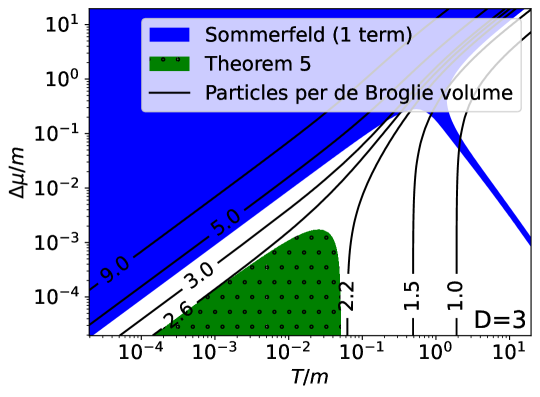
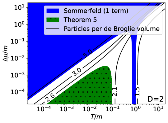
Figure 6: Comparison of two and three dimensional cases of domains of validity in $(T/m,\Delta\mu/m)$-surface ($\Delta\mu\equiv\mu-m$), including relativistic parameter range, of the Sommerfeld expansion (solid blue) and the expansion from Theorem 5 (dotted green), where validity is defined as the computation of $\langle G\rangle_{T}$ having relative error less that $10\%$ for the choice $G(p)=1$.

3.3 Asymptotic Expansion in the Regime $|\mu-m|\ll T\ll m$

One can also use the expansion Eq. (4) to study the regime where $\mu$ approaches $m$ faster than $T$ approaches zero. Mathematically we parameterize this as

$$\mu=m(1+B\widetilde{T}^{1+\gamma})\,,\,\,\,B\in\mathbb{R}\,,\,\,\gamma>0\,.$$ (84)

To proceed, first Taylor expand Eq. (80) to first order in $b$ by differentiating under the integral to obtain

$$-\Gamma(1+n/2)\mathrm{Li}_{1+n/2}(-e^{b})=\int_{0}^{\infty}du\,\frac{u^{n/2}}{1+e^{u-b}}$$ (85)

$$= \int_{0}^{\infty}du\,\frac{u^{n/2}}{e^{u}+1}+b\int_{0}^{\infty}du\,\frac{u^{n/2}}{(e^{u/2}+e^{-u/2})^{2}}+\mathcal{O}(b^{2})$$

$$= (1-2^{-n/2})\Gamma(1+n/2)\zeta(1+n/2)+b\int_{0}^{\infty}du\,\frac{u^{n/2}}{(e^{u/2}+e^{-u/2})^{2}}+\mathcal{O}(b^{2})\,.$$ (86)

See [5] and [7] for in-depth discussion of the computation of Eq. (85). For $n=0$ the leading order term in Eq. (86) has the indeterminate form $0\cdot\infty$ (this case will only be relevant to us when $D=2)$; there one should instead use

$$\int_{0}^{\infty}du\frac{1}{1+e^{u-b}}=\ln(1+e^{b})=\ln(2)+\frac{b}{2}+\mathcal{O}(b^{2})\,.$$ (87)

Now substitute Eq. (85) into Eq. (4) and let $b=B\widetilde{T}^{\gamma}$. We note that the remainder term in Eq. (4) is still $\mathcal{O}(\widetilde{T}^{1+(k+D-2)/2})$ in this case because $b$ remains bounded above (in fact, it remains bounded) as $\widetilde{T}\to 0$; see Remark 2. The expansion Eq. (4) with $k=2$ then simplifies to give the following result.

Theorem 5.

Let $G(p)$ be a $C^{2}$ function on $[0,\infty)$ whose zeroth through $2$nd derivatives are polynomially bounded. Let $\mu=m(1+B\widetilde{T}^{1+\gamma})$ where $B\in\mathbb{R}$, $\gamma>0$, $\widetilde{T}=T/m$.

1. For $D=3$ and with $a_{n}$ is defined by Eq. (58) we have

   $$\int_{0}^{\infty}dp\,p^{2}G(p)f_{FD}(p)$$ (88)

   $$= a_{0}(m)m^{3}(1-2^{-1/2})\frac{\pi^{1/2}}{2}\zeta(3/2)\widetilde{T}^{3/2}-a_{0}(m)m^{3}({2}^{1/2}-1)\frac{\pi^{1/2}}{2}\zeta(1/2)B\widetilde{T}^{3/2+\gamma}$$

   $$+a_{1}(m)m^{3}\frac{\pi^{2}}{12}\widetilde{T}^{2}+\mathcal{O}(\widetilde{T}^{3/2+2\gamma})+\mathcal{O}\left(\widetilde{T}^{5/2}\right)\,\,\,\,\text{as}\,\,\,\widetilde{T}\to 0\,.$$ (89)

2. For $D=2$ and with $a_{n}$ is defined by Eq. (58) we have

   $$\int_{0}^{\infty}dp\,pG(p)f_{FD}(p)$$ (90)

   $$= a_{0}(m)m^{2}\ln(2)\widetilde{T}+\frac{1}{2}a_{0}(m)m^{2}B\widetilde{T}^{1+\gamma}+a_{1}(m)m^{2}(1-2^{-1/2})\frac{\pi^{1/2}}{2}\zeta(3/2)\widetilde{T}^{3/2}$$

   $$+\mathcal{O}\left(\widetilde{T}^{1+2\gamma}\right)+\mathcal{O}\left(\widetilde{T}^{2}\right)\,\,\,\,\text{as}\,\,\,\widetilde{T}\to 0\,.$$ (91)

Remark 3.

When referring to the number of terms in the expansions in Theorem 5 and related results, e.g., in Figure 5, we mean the index $k$ that was used in Eq. (4) to obtain the expansion.

The dominant error term in Eq. (89) and Eq. (91) depends on whether $\gamma<1/2$ or $\gamma\geq 1/2$. To obtain higher order terms in these expansions one simply needs to continue the expansion Eq. (85) to the appropriate higher order before substituting it into Eq. (4); however, we again emphasize that these results are asymptotic expansions and so going to higher order does not necessarily increase the accuracy at a given $T$. When applying Theorem 5 to given values of $\mu$ and $T$, i.e., without reference to any parameterization of the form Eq. (84), we fix $B=1$ if $\mu>m$ and $B=-1$ if $\mu<m$ and then choose the unique $\gamma$ that makes the equality Eq. (84) hold (the case $\mu=m$ was already considered in Section 3.2).

See Figure 5 above for a comparison between the expansion Eq. (89) (green dashed line) and numerical integration of Eq. (88) (solid black line). We also compare with the Sommerfeld expansion Eq. (33) (red dot-dashed line). Note that the Sommerfeld expansion completely fails in the low temperature regime when $\mu$ and $T$ are related by Eq. (84) with $0<\mu-m\ll T$. Under the parameterization Eq. (84), the traditional Sommerfeld expansion is actually seen to be valid at high temperature; we proved this to be the case in Theorem 3 above.

In Figure 6 we again present a comparison between the domain of applicability of the Sommerfeld expansion and Theorem 5. Here we show the number of particles per de Broglie volume in the solid black contours, from which we can see that our new expansion applies in a moderate density regime where quantum effects are non-negligible but that is distinct from the high-density regime where the Sommerfeld expansion applies. The region of validity of Theorem 5 is a bit larger in dimension $D=2$ (bottom frame) than in $D=3$ (top frame).

4 Discussion of Results

We resolved a century long oversight, the understanding of the dilute Fermi-Dirac (FD) quantum domain in which the traditional Sommerfeld expansion fails. We recognize the particle number per de Broglie volume as a critical physical quantity which separates the different FD regimes, i.e., the regions in the $(T/m,(\mu-m)/m)$-plane where different asymptotic expansions apply. We obtain a novel asymptotic expansion that is valid when the particle number per de Broglie volume is moderate (2 to 3 particles), as compared to the low density semiclassical Boltzmann limit (1 particle or less) and the traditional highly degenerate Sommerfeld limit (5 or more particles); see Figure 1. This intermediate density regime was unrecognized in the literature, where often one finds a mere acknowledgement that “the Sommerfeld expansion fails”. In addition, we add to the understanding of the Sommerfeld expansion in the high temperature regime and when $\mu$ is close to $m$.

Our main results in regard to different regimes are as follows, with detailed assumptions found in the referenced theorems, and figure illustrations offered for the nonrelativistic regime in Figure 1, and extension to relativistic regime along with comparisons in Figure 4 and Figure 6:

1. Nonrelativistic degenerate Fermi gas: Regime $T\ll\mu-m\ll m$ considered for dimension $D\geq 2$, with $\Delta\widetilde{\mu}=(\mu-m)/m\to 0^{+}$, while $T$ is constrained by $T=d\Delta\widetilde{\mu}^{1+\gamma}m$, $d,\gamma>0$ (Theorem 2),

   $$\int_{0}^{\infty}dp\,p^{D-1}G(p)(f_{T\neq 0}+\widetilde{f}_{T\neq 0})=\sum_{n=0}^{k-1}da_{n}(m)m^{D}\Delta\widetilde{\mu}^{(n+D)/2+\gamma}$$ (92)

   $$\times\sum_{j=1,\mathrm{odd}}^{\lceil(k-n)/(2\gamma)\rceil-1}2d^{j}\Delta\widetilde{\mu}^{j\gamma}\left(\prod_{\ell=0}^{j-1}[(n+D-2)/2-\ell]\right)(1-2^{-j})\zeta(j+1)$$

   $$+\mathcal{O}\left(\Delta\widetilde{\mu}^{(k+D)/2+\gamma}\right)\;,$$

   $$a_{n}(m)=\frac{1}{n!}\partial_{y}^{n}|_{y=0}\left[(y^{2}+1)(y^{2}+2)^{(D-2)/2}G\left(my\sqrt{y^{2}+2}\right)\right]\,.$$ (93)

   Here $f_{T\neq 0}+\widetilde{f}_{T\neq 0}$ denotes the finite temperature component of the FD distribution as defined in Eq. (7).

2. Relativistic, dense Fermi gas: Regime $\mu\gg T\gg m$ with $T\to\infty$, while $\mu$ is constrained by $\mu=m[1+B(T/m)^{1+\gamma}]$, $\gamma,B>0$ (Theorem 3),

   $$\int_{m}^{\infty}dE\,H(E)f_{FD}(E)=\int_{m}^{\mu}dE\,H(E)$$ (94)

   $$+\sum_{n=1,n\text{ odd}}^{k-2}2(1-2^{-n})\zeta(n+1)T^{n+1}H^{(n)}(\mu)+\mathcal{O}(\mu^{q_{k}}T^{k+1})\;.$$

3. Dilute quantum Fermi gas $D=3$: Regime $|\mu-m|\ll T\ll m$ with $\widetilde{T}=T/m\to 0$, while $\mu$ is constrained by $\mu=m[1+B\widetilde{T}^{1+\gamma}]$, $B\in\mathbb{R}$, $\gamma>0$ (Theorem 5, $D=3$),

   $$\int_{0}^{\infty}dp\,p^{2}G(p)f_{FD}(p)=m^{3}G(0)(1-2^{-1/2})\left(\frac{\pi}{2}\right)^{1/2}\!\!\zeta(3/2)\widetilde{T}^{3/2}$$ (95)

   $$-m^{3}G(0)({2}^{1/2}-1)\left(\frac{\pi}{2}\right)^{1/2}\!\!\zeta(1/2)B\widetilde{T}^{3/2+\gamma}+2m^{4}G^{\prime}(0)\frac{\pi^{2}}{12}\widetilde{T}^{2}$$

   $$+\mathcal{O}(\widetilde{T}^{3/2+2\gamma})+\mathcal{O}\left(\widetilde{T}^{5/2}\right)\;.$$

4. Dilute quantum Fermi gas $D=2$: Regime $|\mu-m|\ll T\ll m$ with $\widetilde{T}=T/m\to 0$, while $\mu$ is constrained by $\mu=m[1+B\widetilde{T}^{1+\gamma}]$, $B\in\mathbb{R}$, $\gamma>0$ (Theorem 5, $D=2$),

   $$\int_{0}^{\infty}dp\,pG(p)f_{FD}(p)=m^{2}G(0)\ln(2)\widetilde{T}$$ (96)

   $$+\frac{1}{2}m^{2}G(0)B\widetilde{T}^{1+\gamma}+m^{3}G^{\prime}(0)(1-2^{-1/2})\left(\frac{\pi}{2}\right)^{1/2}\zeta(3/2)\widetilde{T}^{3/2}$$

   $$+\mathcal{O}\left(\widetilde{T}^{1+2\gamma}\right)+\mathcal{O}\left(\widetilde{T}^{2}\right)\;.$$

Further terms in Eq. (95) and Eq. (96) can be obtained by using the more general result in Theorem 4.

We have also introduced as a supplemental tool a novel form of the FD distribution Eq. (7) that separates the Fermi gas into zero and finite temperature components, see Figure 2. We find this decomposition convenient when deriving asymptotic expansions of finite $T$ effects, as seen in Section 2.

We note that the analysis presented here does not incorporate a number of features that are important in specific physics applications, such as magnetism, spin, particle-antiparticle effects, and cosmological free-streaming distributions. We intend to consider these natural refinements of the methods presented here in future application-oriented work.

Acknowledgments We thank Gordon Baym and John W. Clark for their encouragement to pursue research into the novel form of the Fermi distribution which ultimately lead to this work.

References

- \bibcommenthead
- Bludman and Van Riper [1977] Bludman, S.A., Van Riper, K.A.: Equation of state of an ideal Fermi gas. Astrophysical Journal 212, 859–872 (1977)
- Elze et al. [1980] Elze, H.T., Greiner, W., Rafelski, J.: The relativistic Fermi gas revisited. J. Phys. G 6, 149–153 (1980) https://doi.org/10.1088/0305-4616/6/9/003
- Ferrer and Hackebill [2019] Ferrer, E.J., Hackebill, A.: Thermodynamics of Neutrons in a Magnetic Field and its Implications for Neutron Stars. Phys. Rev. C 99(6), 065803 (2019) https://doi.org/10.1103/PhysRevC.99.065803 arXiv:1903.08224 [nucl-th]
- Kübler [2021] Kübler, J.: Theory of Itinerant Electron Magnetism. Oxford University Press, Oxford, UK (2021). https://doi.org/%****␣novel-fermi-function.bbl␣Line␣100␣****10.1093/oso/9780192895639.001.0001 . 2nd Edition
- Dingle [1957] Dingle, R.: The Fermi-Dirac integrals. Applied Scientific Research, Section B 6(1), 225–239 (1957) https://doi.org/10.1007/BF02920379
- Dingle [1973] Dingle, R.B.: Asymptotic Expansions: Their Derivation and Interpretation. Academic Press, London and New York (1973). https://doi.org/10.1007/978-1-4612-0827-3
- Garoni et al. [2001] Garoni, T.M., Frankel, N.E., Glasser, M.L.: Complete asymptotic expansions of the Fermi–Dirac integrals . Journal of Mathematical Physics 42(4), 1860–1868 (2001) https://doi.org/10.1063/1.1350634 https://pubs.aip.org/aip/jmp/article-pdf/42/4/1860/19314445/1860_1_online.pdf
- Lourenco et al. [2007] Lourenco, O., Dutra, M., Delfino, A., Sa Martins, J.S.: Relativistic Sommerfeld low temperature expansion. Int. J. Mod. Phys. D 16, 285–289 (2007) https://doi.org/10.1142/S021827180701002X
- Wasserman et al. [1970] Wasserman, A., Buckholtz, T.J., DeWitt, H.E.: Evaluation of Some Fermi‐Dirac Integrals. Journal of Mathematical Physics 11(2), 477–482 (1970) https://doi.org/%****␣novel-fermi-function.bbl␣Line␣175␣****10.1063/1.1665160 https://pubs.aip.org/aip/jmp/article-pdf/11/2/477/19230647/477_1_online.pdf
- Fukushima [2014] Fukushima, T.: Analytical computation of generalized Fermi–Dirac integrals by truncated Sommerfeld expansions. Applied Mathematics and Computation 234, 417–433 (2014) https://doi.org/10.1016/j.amc.2014.02.053
- Gil et al. [2022] Gil, A., Segura, J., Temme, N.M.: Complete asymptotic expansions for the relativistic Fermi-Dirac integral. Applied Mathematics and Computation 412, 126618 (2022) https://doi.org/10.1016/j.amc.2021.126618
- Gil et al. [2023] Gil, A., Odrzywołek, A., Segura, J., Temme, N.M.: Evaluation of the generalized Fermi-Dirac integral and its derivatives for moderate/large values of the parameters. Computer Physics Communications 283, 108563 (2023) https://doi.org/10.1016/j.cpc.2022.108563
- Kim et al. [2008] Kim, R., Wang, X., Lundstrom, M.: Notes on Fermi-Dirac integrals. arXiv preprint arXiv:0811.0116 (2008)
- Buterakos et al. [2021] Buterakos, D., Vu, D., Yu, J., Das Sarma, S.: Presence versus absence of two-dimensional Fermi surface anomalies. Phys. Rev. B 103, 205154 (2021) https://doi.org/10.1103/PhysRevB.103.205154
- Kaspi and Beloborodov [2017] Kaspi, V.M., Beloborodov, A.: Magnetars. Ann. Rev. Astron. Astrophys. 55, 261–301 (2017) https://doi.org/10.1146/annurev-astro-081915-023329 arXiv:1703.00068 [astro-ph.HE]
- Ferrer and Hackebill [2023] Ferrer, E.J., Hackebill, A.: The Importance of the Pressure Anisotropy Induced by Strong Magnetic Fields on Neutron Star Physics. J. Phys. Conf. Ser. 2536(1), 012007 (2023) https://doi.org/10.1088/1742-6596/2536/1/012007
- Rafelski and Yang [2021] Rafelski, J., Yang, C.T.: The muon abundance in the primordial Universe. Acta Phys. Polon. B 52, 277 (2021) https://doi.org/10.5506/APhysPolB.52.277 arXiv:2103.07812 [hep-ph]
- Rafelski et al. [2023] Rafelski, J., Birrell, J., Steinmetz, A., Yang, C.T.: A Short Survey of Matter-Antimatter Evolution in the Primordial Universe. Universe 9(7), 309 (2023) https://doi.org/10.3390/universe9070309 arXiv:2305.09055 [hep-th]
- Grayson et al. [2023] Grayson, C., Yang, C.T., Formanek, M., Rafelski, J.: Electron–positron plasma in BBN: Damped-dynamic screening. Annals Phys. 458, 169453 (2023) https://doi.org/10.1016/j.aop.2023.169453 arXiv:2307.11264 [astro-ph.CO]
- Steinmetz et al. [2023] Steinmetz, A., Yang, C.T., Rafelski, J.: Matter-antimatter origin of cosmic magnetism. Phys. Rev. D 108(12), 123522 (2023) https://doi.org/10.1103/PhysRevD.108.123522 arXiv:2308.14818 [hep-ph]
- Letessier and Rafelski [2023] Letessier, J., Rafelski, J.: Hadrons and Quark–Gluon Plasma. Cambridge Monographs on Particle Physics, Nuclear Physics and Cosmology. Cambridge University Press, Cambridge (2023). https://doi.org/10.1017/9781009290753 . Open access. [orig. pub. 2002]
- Rafelski and Yang [2022] Rafelski, J., Yang, C.T.: Reactions Governing Strangeness Abundance in Primordial Universe. EPJ Web Conf. 259, 13001 (2022) https://doi.org/10.1051/epjconf/202225913001 arXiv:2009.05661 [hep-ph]
- Yang and Rafelski [2022] Yang, C.T., Rafelski, J.: Cosmological strangeness abundance. Phys. Lett. B 827, 136944 (2022) https://doi.org/%****␣novel-fermi-function.bbl␣Line␣400␣****10.1016/j.physletb.2022.136944 arXiv:2108.01752 [hep-ph]
- Landau and Lifshitz [1980] Landau, L.D., Lifshitz, E.M.: Course of Theoretical Physics, Volume 5, Statistical Physics, Part 1, 3rd Edition. Pergamon Press, Elmsford, NY (1980)
- Birrell et al. [2013] Birrell, J., Yang, C.-T., Chen, P., Rafelski, J.: Fugacity and Reheating of Primordial Neutrinos. Mod. Phys. Lett. A 28, 1350188 (2013) https://doi.org/10.1142/S0217732313501885 arXiv:1303.2583 [astro-ph.CO]
- Birrell et al. [2014] Birrell, J., Yang, C.-T., Chen, P., Rafelski, J.: Relic neutrinos: Physically consistent treatment of effective number of neutrinos and neutrino mass. Phys. Rev. D 89, 023008 (2014) https://doi.org/10.1103/PhysRevD.89.023008 arXiv:1212.6943 [astro-ph.CO]
- Gradshteyn and Ryzhik [2007] Gradshteyn, I.S., Ryzhik, I.M.: Table of Integrals, Series, and Products, 7th Edition. Academic Press, Burlington, MA (2007)