Financial Table Extraction in Image Documents

Abstract.

Table extraction has long been a pervasive problem in financial services. This is more challenging in the image domain, where content is locked behind cumbersome pixel format. Luckily, advances in deep learning for image segmentation, OCR, and sequence modeling provides the necessary heavy lifting to achieve impressive results. This paper presents an end-to-end pipeline for identifying, extracting and transcribing tabular content in image documents, while retaining the original spatial relations with high fidelity.

1. Introduction

	September 30,	March 31,
	2019	2019
Current liabilities	US$’000	US$’000
Trade payables	7,857,686	6,429,835
Notes payable	1,253,503	1,272,840
Derivative financial liabilities	37,345	74,426
Other payables and accruals	10,428,998	8,942,336
Provisions	715,332	738,688
Deferred revenue	770,229	780,951
Income tax payable	328,442	298,224
Borrowings	2,648,151	1,953,043
	24,039,686	20,490,343

Figure 1. The three steps of tabular extraction from image docs. Top: table identification. Middle: content recovery. Bottom: alignment into tabular format.

Table extraction has long been a persistent problem in automating data collection in the financial service sector. Documents vary in style and content, each being derived from a unique source. This paper concerns itself with the image domain, where the only machine-readable data is pixelated. These financial documents do not have a consistent format and often exhibit high variance in layouts across pages and files. Therefore, financial image documents pose several unique challenges:

1. How can we find a table?

2. How can we recover the content of a table?

3. How can we align the content into a tabular format?

Our proposed pipeline effectively segments the problem into these three sub-tasks. Luckily, deep learning offers several techniques to tackle these sub-problems, and when built in conjunction with classical data structures and algorithms, can be shown to create an effective pipeline for table extraction. But one must ask, why do we need a system like this? First, images are pixelated, a cumbersome format for text extraction and processing. For these formats, there is no way to copy and paste the content. Techniques such as optical character recognition (OCR) or human transcription are required to digitize content into a friendlier format, to ascribe meaning to a set of colored pixels. Hence, this paper proposes an image based pipeline to transcribe tabular information locked in image format into a variety of structured outputs (CSV, Dataframes, or LaTeX).

2. Relevant Background

Table detection is not a new problem. There is an extensive body of prior literature that have used various approaches in detecting tables in images. Kieninger et al. (Dengel and Kieninger, 1998; Kieninger and Dengel, 2001) used a system called T-Recs to take word boundaries and cluster them into a segmentation graph to detect tables. However, it failed in the presence of multi-column layouts. Wang et al. (Yalin Wangt et al., 2001) used the distance between consecutive words as a heuristic in determining table entity candidates, but was tied to a specific layout template. Hu et al. (Hu et al., 1999) proposed an approach involving single columned images. Shafait et al. (Shafait and Smith, 2010) looked at heterogeneous documents, and their system was eventually integrated into Tesseract. Tupaj et al. (Tupaj et al., 1996) searches the image for sequences of table-like lines based on header keywords. Harit et al. (Harit and Bansal, 2012) used unique table start and trailer patterns, but fails when the patterns are unique. Gatos et al. (Gatos et al., 2005) uses the area of intersection between horizontal and vertical lines to reconstruct the intersectional pairs. However, this system relies on the visual cues provided by strict, defining table borders. Hidden Markov Models were proposed by Costa e Silva (e. Silva, 2009), and Kasar (Kasar et al., 2013) locates tables through column and row separators with Support Vector Machines. Other methods were explored by Jahan et al. (Jahan and Ragel, 2014) with word spacing and line height thresholds for table localization. Hybrid approaches attempt to discover table candidate regions, as in Anh et al. (Anh et al., 2015). Finally, deep learning methods were presented in Hao et al. (Hao et al., 2016) regional proposal network using CNNs, and Gilani et al. (Gilani et al., 2017) adapted the Faster R-CNN architecture to segment table regions in a given image. We propose a pipeline for financial image documents that identifies table boundaries, extracts text content, and aligns table cells using spatial, textual, and sequential features.

3. Table Detection

Table detection converts PDF files into images and detects table boundaries for each page as a list of coordinates $(x1,x2,y1,y2)$. Even though this is a detection task, we adopt a semantic segmentation approach for two reasons. First, object detection models are designed to detect multiple categories of objects in the same image, as the case for benchmark detection tasks such as COCO (Lin et al., 2014). But here we only care about one type of object, tables. Semantic segmentation solves the problem of classifying each pixel into categories, i.e. segmenting the image into different regions. Therefore our problem can be framed as a segmentation task with two categories, the table region and other. Second, object detection models (especially two-stage ones like Faster R-CNN (Ren et al., 2015) and Cascade R-CNN (Cai and Vasconcelos, 2017)) are much heavier than the semantic segmentation model U-Net (Ronneberger et al., 2015), in terms of both training and inference time. Since a segmentation model’s output masks can be of any shape, post-processing is performed to convert them into proper bounding boxes.

3.1. Models

The first step is to convert arbitrary length PDFs into single page images. We used ImageMagick’s convert tool at 300 dpi grayscale with no compression loss (PNG). We chose 300 dpi in order to ensure that images during the OCR phase (§4) remain at an acceptable quality for text extraction.

3.1.1. Classification Model

In financial documents, not all pages have tables. Depending on the corpus, the proportion of empty pages (i.e., no tables) is about half. Although segmentation models can deal with empty pages by predicting zero tables after post-processing, a classification model works better for the task of identifying empty pages. Therefore we use a binary table classification model to filter pages without tables before feeding the remaining pages into the segmentation model. Annotating pages as a binary task is much cheaper than annotating table locations for segmentation, so we can easily create a large training set covering a variety of non-table pages, such as those with different types of pictures and graphs. Inference is twice as fast with the classification model over the segmentation model. Our model uses the Inception-ResNet v2 (Szegedy et al., 2016) convolution base with input size $384\times 288\times 1$ plus a dense layer of dimension 256. Light augmentation was applied in training: random zoom within $\pm 10\%$ and random horizontal/vertical shift within $\pm 5\%$ to imitate poor quality scans.

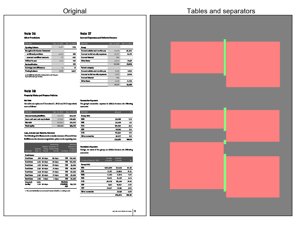
Figure 2. The separator trick: when tables are close to each other, generate a third class, separator (light green), from annotated table boxes (red).

3.1.2. Segmentation Model

Our pipeline adopts U-Net (Ronneberger et al., 2015), which was originally developed for biomedical image segmentation and widely used in various domain tasks such as autonomous driving (Siam et al., 2018) and satellite imagery segmentation (Demir et al., 2018; Iglovikov et al., 2017). In particular, we used a U-Net architecture with DenseNet-169 (Huang et al., 2017) backbone and softmax activation, similar to the winning solution of 2018 Data Science Bowl (Caicedo et al., 2019). The input size is $384\times 288\times 3$. The loss function is a combination of categorical cross entropy (60%) and dice coefficient loss (20% each for the table and separator channels) (Sudre et al., 2017). For augmentation, we applied 2° random rotation and 0.01 shear intensity to imitate low-quality scans. A limitation of applying semantic segmentation to solve object detection problems is that the model does not differentiate instances of the same object type—semantically, they are the same object. Therefore, the model would struggle when multiple objects of the same type are close together, or even touching. A common trick used in nucleus segmentation for biomedical microscopy image analysis is to add a boundary class, resulting in a 3-class semantic segmentation task: background, nucleus boundary, and inside nucleus (Cui et al., 2019; Caicedo et al., 2019). Inspired by this, we add separators between closely located tables, making our problem 3-class: table, separator, and other. We do not do full table boundaries as in nucleus segmentation because in a typical nucleus microscopy image, there are dozens of nuclei squeezed together taking up most of the area, making the full boundary necessary. But in our case, all tables are rectangular and most are not in close proximity to others. Therefore we only need to add separators when necessary, as in Figure 2. After annotation, we used scikit-image’s (van der Walt et al., 2014) dilation and watershed functions to automatically generate the separators. Separators appeared in 13.4% of our annotated set.

3.1.3. Post-processing

Thresholding. The raw output of U-Net is the probability of each pixel belonging to a table. A threshold can convert these into a binary mask: the smaller the threshold the larger the mask and vice versa. We tuned the threshold on our validation set such that output masks have maximal intersection over union (IOU) with ground truth bounding boxes. The optimal threshold is 0.7 at 0.84 IOU.

Separating tables. We use scikit-image to separate the raw masks into different connected regions. Each connected mask is a table candidate. We remove masks that are smaller than 1% of total image area. This is based on the observation that such masks are generally noise as all tables are larger than 1% of the whole page.

Rectanglization. Most individual raw masks are near rectangular. We need to convert them into proper bounding boxes. We do this by taking the minimal enclosing rectangle for each raw mask. The resulting bounding box is always larger than the raw mask. But since we used tight bounding boxes when annotating tables, the results turned out to be good for most cases (see §3.3).

3.2. Dataset and Labeling

We sampled 10,000 pages from a collection of 9,985 financial documents, including annual reports, prospectus documents and shareholder meeting notes published by international companies in various sectors such as commodities, banking, and technology. The dataset was curated for its diversity of content and reporting style. Pages were labeled as either having tables (4,593) or no tables (5,407). 8,000 are used as the training set and 2,000 for validation. Separately, for segmentation, we labeled the bounding boxes for all tables on 909 random pages with tables using the annotation tool LabelMe (Wada, 2016). There were 1,660 tables in total, or 1.8 tables per page. The max number of tables on a page was 10. The U-Net model is trained on a smaller set comprised of 749 pages with 160 for validation, for two reasons. First, for classification, each annotated page only provides 1 bit of information (has a table or not), but a U-Net model can learn more information from a fully annotated segmentation page—each pixel is 1 bit of information (this pixel belongs to a table or not). Second, annotating bounding boxes is more time-consuming than annotating whether a page contains tables. After development, we selected another 1,000 random pages to test the robustness of the pipeline. We did not annotate bounding boxes because IOU is not sufficient to tell whether the detection is satisfactory on a given page, e.g. predicting extra blank surrounding area is more tolerable than missing the table header. Instead, we plotted the predicted bounding boxes on each page (figures 3—10) and judged if the detection was fully correct, partially correct, or incorrect.

Figure 3. Full Success: Border Lines

Figure 4. Full Success: No Border Lines

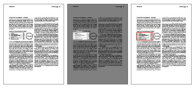
Figure 5. Full Success: Inline Table

Figure 6. Full Success: Stacked Tables

Figure 7. Partial Success: Multiple Tables

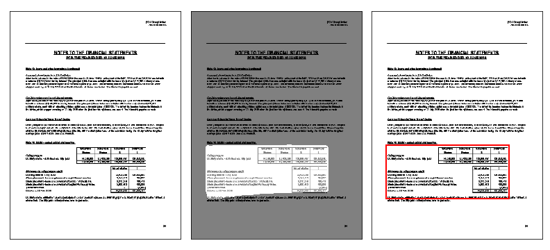
Figure 8. Partial Success: Multiple Tables

Figure 9. Partial Success: Nearby Non-Tabular Text

Figure 10. Partial Success: Incomplete Table

3.3. Results

For the classification model, recall is more important than precision: false positives are acceptable since the downstream U-Net model, with post-processing, has the ability to predict no tables on a page; but false negatives mean a page with tables is thrown away before going further in the pipeline. We tuned the threshold on the validation set such that recall is 0.995 and precision is 0.871.

We examined the pipeline’s output on 1,000 test pages. On the test set, recall is 0.993 and precision is 0.910. Note that recall and precision are table level metrics. On the page-level, 83% were completely correct, followed by 9.5% covering multiple tables, 5.9% covering nearby text, and 1.6% representing other errors. Note that the latter three cases are still considered partially correct.

Figures 3—6 show some correct cases. Figure 3 is the easiest: tables with borders on all sides, resulting in near rectangular masks. Tables in figure 4 either have few or no borders, resulting in non-rectangular masks. Nonetheless, the masks cover all the table’s content and post-processing recovers the correct area. Figure 5 is an inline table, and the segmentation has some holes in the output mask, which post-processing handles easily. Figure 6 are the cases where two tables are located next to each other with minimal space in between. The separator trick is crucial for such cases—the results were much worse before. Here, the segmentation model successfully separated the tables’ masks even though the shapes are not perfect.

Figures 7—10 shows partially correct cases. The most common error is the accidental merger of multiple tables. In figure 7, there are two tables with no space or text between them. Neither table has borders. The segmentation model predicted a merged blob which was post-processed into a single bounding box. In figure 8, there are two inline tables next to each other, and the model predicted a single bounding box covering both tables, plus additional text on the left. Another issue is when the predicted bounding box covers nearby text, as shown in figure 9. The top bounding box includes a line of text below and the top-right page header. Figure 10 is an example of a less common case, where for very wide but short tables, the segmentation model missed some columns if spacing between columns is large. We want to emphasize that none of the partially correct examples are a complete failure. Most examples can be handled by downstream steps to different degrees, but we were conservative in evaluation and did not count them as completely correct, to give a fair assessment of the detection models.

4. Table Extraction

4.1. Tesseract OCR

Given the coordinates of a segmented table, we can extract textual information alongside positional metadata from images with Tesseract OCR. It is a vital component that bridges the gap between table detection and alignment. Tesseract utilizes an LSTM-based engine to predict the character for a given segment of pixels, built alongside line and word finding algorithms (Smith, 2007). In addition, Tesseract provides practical tools for script, language, and orientation detection, allowing us to extract content in other languages, or content that is rotated (Smith, 2007; Unnikrishnan and Smith, 2009). In addition, Tesseract provides useful layout information for lines, blocks, and word boundaries, which is convenient in organizing text into tabular format (Smith, 2009).

4.2. Preprocessing Pipeline

Given the boundaries of a segmented table, our preprocessing pipeline to enhance the image before OCR consists of three major components: Otsu Thresholding (Otsu, 1979), Automatic Orientation Correction, and Morphological Kernel Filtering. Prior to these steps, we also crop and pad the region of interest to avoid boundary issues. Our implementation is built from well-known computer vision recipes using OpenCV (Bradski, 2000).

Table 1. Additional Table Pipeline Examples

	Original	Segmentation Mask	OCR Input	Final Alignment
A				3 months ended 6 months ended 3 months ended 6 months ended September 30, September 30, September 30, 2019 2019 2018 2018 (unaudited) (unaudited) (unaudited) (unaudited) Note US$’000 US$’000 Revenue 2 13,521,989 26,034,142 13,379,809 25,292,534 Cost of sales (11,339,441) (21,803,203) (11,585,705) (21,866,758) Gross profit 2,182,548 4,230,939 1,794,104 3,425,776 Selling and distribution expenses (777,804) (1,541,133) (654,739) (1,308,943) Administrative expenses (584,534) (1,195,250) (514,955) (1,000,134) Research and development expenses (318,028) (647,343) (312,341) (622,236) Other operating expenses - net (60,438) (62,818) (22,522) (24,543) Operating profit 3 441,744 784,395 289,547 469,920 Finance income 4(a) 10,602 24,474 6,176 11,474 Finance costs 4(b) (136,218) (251,240) (81,732) (153,580) Share of losses of associates and joint ventures (6,072) (7,448) (694) (1,721) Profit before taxation 310,056 550,181 213,297 326,093 Taxation 5 (66,417) (114,600) (39,815) (67,291) Profit for the period 243,639 435,581 173,482 258,802 Profit/(loss) attributable to: Equity holders of the Company 202,194 364,421 168,403 245,447 Perpetual securities holders 13,440 26,880 13,440 26,880 Other non-controlling interests 28,005 44,280 (8,361) (13,525) 243,639 435,581 173,482 258,802 Earnings per share attributable to equity holders of the Company Basic 6(a) US 1.69 cents US 3.06 cents US 1.41 cents US 2.06 cents Diluted 6(b) US 1.62 cents US 2.94 cents US 1.40 cents US 2.06 cents Dividend 7 96,640 92,071
B				(d) Analysis of revenue by geography 6 months 6 months ended ended September 30, September 30, 2019 2018 US$’000 US$’ 000 China 5,507,563 6,268,642 AP 6,013,844 4,726,400 EMEA 5,890,192 6,074,567 AG 8,622,543 8,222,925 26,034,142 25,292,534 (e) Analysis of revenue by timing of revenue recog… 6 months 6 months ended ended September 30, September 30, 2019 2018 US$’000 US$’ 000 Point in time 25,433,884 24,826,983 Over time 600,258 465,551 26,034,142 25,292,534 (f) Other segment information IDG DCG Total 2019 2018 2019 2018 2019 2018 US$’000 US$”000 US$’000 US$’000 US$’000 US$’000 For the six months ended September 30 Depreciation and amortization 258,842 228,961 116,345 102,790 375,187 331,751 Finance income 10,296 10,093 1,238 96 11,534 10,189 Finance costs 95,280 83,871 7,876 8,917 103,156 92,788 Additions to non-current assets (Note) 344,076 484,027 171,656 48,488 515,732 532,515 Note: Excluding other non-current assets and i…
C				{a) DVtails of otner payables and accruals are as… September 30, March 31, 2019 2019 US$’000 US$’ 000 Accruals 1,962,647 1,969,914 Allowance for billing adjustments Ci) 1,769,566 1,650,226 Contingent consideration (Note 12(a)) 117,204 - Other payables (ii) 6,579,581 5,322,196 10,428,998 8,942,336 Environmental Warranty restoration Restructuring Total Us$’000 Us$’000 US$’000 Year ended March 31, 2019 At the beginning of the year 1,081,218 8,919 54,053 1,144,190 Exchange adjustment (37,163) (274) (1,991) (39,428) Provisions made 807,636 14,545 - 822,181 Amounts utilized (875,413) (14,403) (36,576) (926,392) Acquisition of subsidiaries - 24,510 - 24,510 976,278 33,297 15,486 1,025,061 Long-term portion classified as non-current liabilities (254,601) (31,772) - (286,373) At the end of the year 721,677 1,525 15,486 738,688 Period ended September 30, 2019 At the beginning of the period 976,278 33,297 15,486 1,025,061 Exchange adjustment (16,863) 831 (91) (16,123) Provisions made 398,897 9,910 - 408,807 Amounts utilized (390,848) (8,621) (15,395) (414,864) 967,464 35,417 - 1,002,881 Long-term portion classified as non-current liabilities (254,769) (32,780) - (287,549) At the end of the period 712,695 2,637 - 715,332

4.2.1. Automatic Orientation Correction

We use Tesseract’s automatic orientation detection algorithm (Unnikrishnan and Smith, 2009) to determine the angle of the text in the image. This is necessary because some tables are in landscape mode, but are not properly rotated in the document itself. Therefore, some images are rotated at $90$ or $270$ degree angles. We do not rotate if the detection returns $0$ or $180$, as it has been our observation that $180$ is given in error and assume that no table is completely flipped. It is important to note that we also preserve the dimensions and scope of the rotated table by adjusting the rotation matrix with a translation term.

4.2.2. Morphological Kernel Filtering

OCR systems are sensitive to noise, and in particular table borders that can accidentally register as a character or word. To mitigate this problem, we use a filtering algorithm based on structuring elements and morphological operators to remove lines from a table. A structuring element, or kernel, is a preset pattern represented by a binary grid. For our experiments, the kernel size was set to $50\times i$ for the horizontal direction, and to $i\times 50$ for the vertical direction, with $i\in\{1,2\}$. We set the main dimension to $50$ in order to capture long continuous streaks and ignore smaller character strokes, for both the vertical and horizontal directions. The basic operators for morphological transforms are erosion and dilation. For erosion, a binary image thins out, as the pixel will remain a $1$ if and only if the window at said pixel exactly matches the kernel. Dilation, in contrast, will expand the object if any pixel in the window matches an element in the kernel. Opening is erosion followed by dilation. The process of extracting lines in a single direction (horizontal or vertical) is independent from the other. The algorithm simply applies the summed result of an opening operator. Hence, a mask for each direction is created. These masks are added together, dilated to increase the line coverage, and slightly blurred using a small $3\times 3$ filter. Finally, we remove the lines through a bitwise AND operation on the original image and mask, removing vertical and horizontal strokes from the table.

4.3. Extracted Metadata

Tesseract provides crucial metadata to manipulate the OCR results into a structured table: the word itself, the bounding box (left, top, width, height), the confidence score, and finally, sequential layout data (paragraph, line, and word identifiers). We have found that the paragraph and line fields roughly correspond to horizontally aligned text fields, and the word position is useful for a rough ordering of a line’s text. However, the key data is the bounding box and text information. We drop low confidence OCR results to remove excess noise from the alignment stage. This significantly reduces false triggers and catastrophic misalignments.

5. Table Alignment

5.1. Alignment Data Structure & Algorithm

We approach the concept of alignment as creating a pool of disjoint sets, where each set can correspond to a column. This idea of unifying individual text segments into a set is inspired by Knight’s work on unification (Knight, 1989). Luckily, the disjoint-set or union-find structure marries sub nodes into co-relating trees that represent a set efficiently (Cormen et al., 2009; Galler and Fisher, 1964). With path compression and union by rank, we ensure the height of these trees are shallow, and has been proven to provide a search and merge time complexity of $O\left(\alpha\left(n\right)\right)$, where $\alpha\left(n\right)$ is the inverse Ackermann function  (Fredman and Saks, 1989; Hopcroft and Ullman, 1973; Tarjan, 1975, 1979; Tarjan and van Leeuwen, 1984). Since the inverse Ackermann function is bounded to be less than $4$ for practical sizes of $n$, this implies the structure performs operations approximately in constant time (Cormen et al., 2009).

The algorithm uses the Intersection Over Union to trigger the merging of two trees based on the width overlap of their member cells. This avoids merging two non-aligned cells and its children. When we merge 2 cells, all other previously merged cells are now co-related without any additional work. Using this lookup structure, we can sort our sets and assemble them into a grid by iterating through the rows and placing each column cell in its most plausible alignment. This is trivial since we now have the rough dimensions of the grid we are making from unique sets created by the union-find structure. The result is a structured dataframe that can be exported into various outputs such as CSV, Excel, or LaTeX for further downstream applications or direct embedding.

We use our labels to develop a upper bound on the number of true columns and cells for a given table. We calculate the symmetric mean absolute percentage error (SMAPE) per table to obtain error distributions for each model (Meade and Armstrong, 1986; Flores, 1986). SMAPE is bounded between $0$ and $200\%$, and under-forecasting is penalized more than over-forecasting. Effectively, this means that we prefer errors that will overestimate cells since underestimating leads to catastrophic mergers that are harder to correct. We report the relevant quantiles and maximum error rates, alongside the percentage of perfect alignments, i.e. zero error.

5.2. Column Segmentation

Table alignment relies on intelligently organizing disjoint segments of words into a collection of rows and columns. Rows are already organized by unique line identifiers from Tesseract. For columns, we explored different model schemes to provide rough segments that can be merged into larger cells to help in the alignment process.

We sampled 3,640 suspected tables from the detection pipeline, drawn from a collection of unstructured financial documents that included financial statements, compliance certificates, management presentations, and more. We hand labeled cell boundaries on tables with the lines removed (§4.2.2). Interestingly, 3,038 (83.5%) tables would be considered valid by human labelers. The invalid cases were graphs, pictures, or bullet lists misidentified as a table. Filtering our dataset on these tables, we ran the OCR pipeline to receive word metadata. Together, these tables have 99,000 unique tokens, and 510,000 individual segments to align. To make training tractable, we employ a 2 step fallback tokenization scheme. First, we include a token if it has a cumulative frequency over 75. Secondly, if the token fails to meet this threshold, we instead use its combined POS tag generated from spaCy. A combined POS tag is all the individual POS tags concatenated together, i.e. (45%) becomes PUNCT-NUM-SYM-PUNCT (POS length 4). If a POS tag does not have a frequency over 20, or the combined length is over 7, we treat it as an unknown token. This method yielded 881 unique token tags. For spatial information, we define 4 main features: distance to next token, distance to previous token, start of a row, and end of a row. Only 2 can be active at a time, since a token at the start of a row does not have a distance to a previous token, and vice versa. Distances are normalized to the maximum line length between the left and right most text segments.

5.2.1. Task Formulation

It is useful to think of a table as a sequence of sequences. In other words, each table $t$ consists of a sequence of $n$ rows, $r_{0},\ldots,r_{i},\ldots,r_{n}$, with each row consisting of a sequence of text and spatial features, $r_{i}=\left[r_{i0}\ldots r_{ij}\ldots r_{im}\right]$. Each row can be of varying length. We can predict column segmentations as a binary output for a single segment as follows: 1 if its the end of a segment, 0 otherwise. Hence, the task is reduced to a simple binary classification problem.

(1) $$\centering\small\begin{array}[]{cccccc}Less&imputed&interest&{}\hfil&(174,862.64)&{}\hfil\\ 0&0&\textbf{1}&{}\hfil&\textbf{1}&{}\hfil\\ Less&imputed&interest&\mathbf{\langle}\mathbf{SEG}\mathbf{\rangle}&(174,862.64)&\mathbf{\langle}\mathbf{SEG}\mathbf{\rangle}\\ \end{array}\@add@centering$$

5.3. Model Arsenal

5.3.1. Method 0: Unsupervised

Our baseline comparison will be no model, and forcing our alignment algorithm to find disjoint columns purely on word segments in an unsupervised setting.

5.3.2. Method 1: Feedforward

To test if a recurrent model is necessary, we experimented with a five layer deep feedforward model that makes predictions on a given feature set. We tested the effectiveness of token tag embeddings versus spatial features. For combining the two, we use a linear layer to project the 4 spatial features to an intermediary embedding of size 16, concatenated to the token tag embedding, and feed the joint representation into the downstream feedforward model. Each layer has a hidden size of 32, with a ReLU activation.

Table 2. Performance metrics per model. Considering each table as an instance, error is measured as number of detected cells versus actual number of cells. The percentiles indicate the SMAPE for this measure. MCC indicates the correlation between no. of identified and actual cells. % Perfect indicates the percentage of tables that were perfectly rendered (no errors).

Model	No. Params	10%	25%	50%	75%	90%	Max	% Perfect	MCC	Section
Unsupervised	0	66.67	91.00	116.65	137.50	155.56	196.74	0.46	-	§ 5.3.1
Feedforward: Spatial	2,769	8.00	31.58	66.67	90.91	116.67	196.14	6.88	0.906	§ 5.3.2
Feedforward: Token	16,801	8.00	27.79	50.00	80.00	110.41	196.61	6.48	0.623	§ 5.3.2
Feedforward: Token + Spatial	17,393	3.77	22.81	47.97	75.86	109.05	195.83	8.85	0.947	§ 5.3.2
LSTM: Row-wise	27,025	0.77	20.98	43.48	70.27	100.00	194.24	10.01	0.953	§ 5.3.3
LSTM: Local Table	27,025	0.00	19.29	41.28	69.29	100.00	195.05	10.50	0.951	§ 5.3.4
LSTM: Swapped Local Table	27,025	0.00	20.41	42.52	70.27	100.00	193.90	10.17	0.954	§ 5.3.5
LSTM: Global Table	27,025	0.00	20.00	42.90	69.65	100.00	193.53	10.30	0.953	§ 5.3.6
Transformer: Row-wise	27,153	0.00	18.18	41.88	69.37	100.00	194.24	10.57	0.950	§ 5.3.7
Transformer: Global Table	27,153	2.35	22.22	46.15	73.68	105.20	195.05	9.71	0.949	§ 5.3.8
Transformer: Recurrent	35,761	0.00	22.22	44.44	71.40	101.66	194.54	10.04	0.951	§ 5.3.9

Figure 11. LSTM: Row-wise

Figure 12. LSTM: Local Table

Figure 13. LSTM: Swapped Hidden State Propagation

Figure 14. LSTM: Global Table

Figure 15. Transformer: Row-wise

Figure 16. Transformer: Recurrent

5.3.3. Method 2: LSTM: Row-wise

A baseline approach is to assume independence amongst the rows. The model is simple: embed the tokens and spatial features, feed the sequence into a 2-layer bidirectional LSTM, and use a linear layer to make segment predictions. With bidirectional layers, we give each token access to neighboring signals to predict whether a new column starts or not.

5.3.4. Method 3: LSTM: Local Table

Tables are sequences of sequences, and to assume independence on individual sequences is hearsay. When segmenting a table, readers do not focus on a single row but makes use of the context surrounding it. Hence, a simple yet effective improvement to induce joint row modeling is to allow for hidden state propagation between the rows, inspired by NMT models (Cho et al., 2014; Sutskever et al., 2014). This deep transition between rows is done by passing the bidirectional hidden states onto the next sequence, using it as the initial hidden vector (Pascanu et al., 2013). Hence, the next row will be able to process the context not only within itself, but build upon what has already been previously seen above it, but be able to attend locally.

5.3.5. Method 4: LSTM: Swapped Hidden State Propagation

Another experimental model can be developed by swapping the forward and reverse hidden states between rows. The assumption behind this model is that recurrent networks are biased towards the most recently seen input. Hence, during the forward computation in the next row, our hidden states encode the context from the end of the previous row. By swapping the hidden states, we ensure that the forward LSTM will receive the context from the beginning of the previous row, which matches the same column pattern.

5.3.6. Method 5: LSTM: Global Table

Unlike the previous cases, where we only operate a bidirectional on the row before propagating the hidden state information to the next, the global model processes the entire table as a singular sequence. So, for a segment in the first row, it incorporates information from the tokens before it in the same row, and all further table tokens downstream in the reverse direction. Hence, it has a global scope over the previous localized models.

5.3.7. Method 6: Transformer: Row-Wise

In recent years, Vaswani et al. (Vaswani et al., 2017) introduced a completely new paradigm for sequence modeling, the transformer. Instead of iterative computation and propagating hidden states, a transformer uses a self-attention mechanism for a key, value, and query. For our purposes, we incorporate the encoder architecture that can operate on a single row and produce independent column alignments, for a direct comparison to the row-wise LSTM model.

5.3.8. Method 7: Transformer: Global Table

We also feed the entire table as a singular sequence. Hence, the multi-head attention can look throughout different rows and jointly make predictions for probable column segmentations. This is considered the global approach to joint table modeling.

5.3.9. Method 8: Transformer: Recurrent

However, we again encounter the same issue of a global over local approach to joint modeling. Hence, we experiment with a version of the transformer decoder that can be both recurrent and attend locally for each row. In the original decoder, a target embedding sequence would mix with the output of the encoder for a given source sentence. However, using the traditional encoder-decoder architecture would only provide pairwise row training. To achieve a joint model, we refeed the decoder’s output in place of the original encoder’s input. Hence, the decoder can first attend locally to the row in the first multi-head attention layer, then use the memory of the previous step as the key and value. To initialize the memory state, we allow for a globally learned vector that can be expanded to the correct sequence length.

5.3.10. Experiment Details

We used a 50/50 train-validation split, resulting in two equal sets of 1,519 tables. Models were trained using the logistic loss on the segments directly. We used the Adam optimizer (Kingma and Ba, 2014) with $\alpha=0.01$ and trained for 640 parameter updates, saving the model with the best validation matthews correlation coefficient (MCC) (Matthews, 1975). This metric is a balanced measure given our class imbalance was 44% positive, 56% negative. Interestingly, both sets achieved similar MCC scores indicating that our training set accurately represents the average use case.

5.3.11. Pipeline Incorporation

In order to integrate our model into the alignment pipeline, we first convert the text from the Tesseract metadata into the 881 valid tokens. Next, we calculate the spatial information for each segment. We query our trained model with these features, and receive a prediction per segment. Using these, we concatenate segments that are predicted to be merged together.

5.4. Alignment Evaluation & Discussion

Several trends are apparent from the results presented in Table 2. First, sequential modeling out performs both feedforward models and the unsupervised approach. Second, LSTM’s benefit from seeing the full table, unlike transformers that do better in a local scope. Transformer-based models may provide too much access to each segment during the MHA, unlike LSTM’s that bias towards a segments local neighborhood. Finally, local joint table modeling outperforms global modeling, as our models can attend to the content that is most relevant, without additional noise from a larger scope. Therefore, the best model for column segmentation, in conjunction with out alignment algorithm, is the LSTM: Local Table.

6. Conclusion

This paper has outlined an end-to-end pipeline to discover, extract, and format tabular content from image documents, with high fidelity. Leveraging advanced deep learning techniques across several sub-fields has enabled us to effectively solve each sub-task, culminating in a strong pipeline that provides a valuable transcription service for tabular data. We foresee this pipeline as integral to many downstream applications. For instance, table values can now be indexed by aligning the row field and column header to a particular value. Rendered excel sheets can be quickly corrected by users, and directly embedded to financial projections and equations.

References

- (1)
- Anh et al. (2015) T. T. Anh, N. In-Seop, and K. Soo-Hyung. 2015. A hybrid method for table detection from document image. In 2015 3rd IAPR Asian Conference on Pattern Recognition (ACPR). 131–135. https://doi.org/10.1109/ACPR.2015.7486480
- Bradski (2000) G. Bradski. 2000. The OpenCV Library. Dr. Dobb’s Journal of Software Tools (2000).
- Cai and Vasconcelos (2017) Zhaowei Cai and Nuno Vasconcelos. 2017. Cascade R-CNN: Delving into High Quality Object Detection. arXiv:cs.CV/1712.00726
- Caicedo et al. (2019) Juan C Caicedo, Allen Goodman, Kyle W Karhohs, Beth A Cimini, Jeanelle Ackerman, Marzieh Haghighi, CherKeng Heng, Tim Becker, Minh Doan, Claire McQuin, et al. 2019. Nucleus segmentation across imaging experiments: the 2018 Data Science Bowl. Nature methods 16, 12 (2019), 1247–1253.
- Cho et al. (2014) Kyunghyun Cho, Bart van Merrienboer, Caglar Gulcehre, Dzmitry Bahdanau, Fethi Bougares, Holger Schwenk, and Yoshua Bengio. 2014. Learning Phrase Representations using RNN Encoder-Decoder for Statistical Machine Translation. arXiv:cs.CL/1406.1078
- Cormen et al. (2009) Thomas H. Cormen, Charles E. Leiserson, Ronald L. Rivest, and Clifford Stein. 2009. Introduction to Algorithms, Third Edition (3rd ed.). The MIT Press.
- Cui et al. (2019) Yuxin Cui, Guiying Zhang, Zhonghao Liu, Zheng Xiong, and Jianjun Hu. 2019. A deep learning algorithm for one-step contour aware nuclei segmentation of histopathology images. Medical & biological engineering & computing 57, 9 (2019), 2027–2043.
- Demir et al. (2018) Ilke Demir, Krzysztof Koperski, David Lindenbaum, Guan Pang, Jing Huang, Saikat Basu, Forest Hughes, Devis Tuia, and Ramesh Raska. 2018. Deepglobe 2018: A challenge to parse the earth through satellite images. In 2018 IEEE/CVF Conference on Computer Vision and Pattern Recognition Workshops (CVPRW). IEEE, 172–17209.
- Dengel and Kieninger (1998) Andreas Dengel and Thomas Kieninger. 1998. A Paper-to-HTML Table Converting System.
- e. Silva (2009) A. C. e. Silva. 2009. Learning Rich Hidden Markov Models in Document Analysis: Table Location. In 2009 10th International Conference on Document Analysis and Recognition. 843–847. https://doi.org/10.1109/ICDAR.2009.185
- Flores (1986) Benito E Flores. 1986. A pragmatic view of accuracy measurement in forecasting. Omega 14, 2 (1986), 93 – 98. https://doi.org/10.1016/0305-0483(86)90013-7
- Fredman and Saks (1989) M. Fredman and M. Saks. 1989. The Cell Probe Complexity of Dynamic Data Structures. In Proceedings of the Twenty-First Annual ACM Symposium on Theory of Computing (Seattle, Washington, USA) (STOC ’89). Association for Computing Machinery, New York, NY, USA, 345–354. https://doi.org/10.1145/73007.73040
- Galler and Fisher (1964) Bernard A. Galler and Michael J. Fisher. 1964. An Improved Equivalence Algorithm. Commun. ACM 7, 5 (May 1964), 301–303.
- Gatos et al. (2005) Basilios Gatos, Dimitrios Danatsas, Ioannis Pratikakis, and Stavros J. Perantonis. 2005. Automatic Table Detection in Document Images. In Proceedings of the Third International Conference on Advances in Pattern Recognition - Volume Part I (Bath, UK) (ICAPR’05). Springer-Verlag, Berlin, Heidelberg, 609–618. https://doi.org/10.1007/11551188_67
- Gilani et al. (2017) Azka Gilani, Shah Rukh Qasim, Imran Malik, and Faisal Shafait. 2017. Table Detection Using Deep Learning. https://doi.org/10.1109/ICDAR.2017.131
- Hao et al. (2016) L. Hao, L. Gao, X. Yi, and Z. Tang. 2016. A Table Detection Method for PDF Documents Based on Convolutional Neural Networks. In 2016 12th IAPR Workshop on Document Analysis Systems (DAS). 287–292.
- Harit and Bansal (2012) Gaurav Harit and Anukriti Bansal. 2012. Table Detection in Document Images Using Header and Trailer Patterns. In Proceedings of the Eighth Indian Conference on Computer Vision, Graphics and Image Processing (Mumbai, India) (ICVGIP ’12). Association for Computing Machinery, New York, NY, USA, Article 62, 8 pages. https://doi.org/10.1145/2425333.2425395
- Hopcroft and Ullman (1973) J. E. Hopcroft and J. D. Ullman. 1973. Set Merging Algorithms. SIAM J. Comput. 2, 4 (1973), 294–303. https://doi.org/10.1137/0202024 arXiv:https://doi.org/10.1137/0202024
- Hu et al. (1999) Jianying Hu, Ramanujan S. Kashi, Daniel P. Lopresti, and Gordon Wilfong. 1999. Medium-independent table detection. In Document Recognition and Retrieval VII, Daniel P. Lopresti and Jiangying Zhou (Eds.), Vol. 3967. International Society for Optics and Photonics, SPIE, 291 – 302. https://doi.org/10.1117/12.373506
- Huang et al. (2017) Gao Huang, Zhuang Liu, Laurens Van Der Maaten, and Kilian Q Weinberger. 2017. Densely connected convolutional networks. In Proceedings of the IEEE conference on computer vision and pattern recognition. 4700–4708.
- Iglovikov et al. (2017) Vladimir Iglovikov, Sergey Mushinskiy, and Vladimir Osin. 2017. Satellite Imagery Feature Detection using Deep Convolutional Neural Network: A Kaggle Competition. arXiv:cs.CV/1706.06169
- Jahan and Ragel (2014) M. A. C. A. Jahan and R. G. Ragel. 2014. Locating tables in scanned documents for reconstructing and republishing. In 7th International Conference on Information and Automation for Sustainability. 1–6. https://doi.org/10.1109/ICIAFS.2014.7069552
- Kasar et al. (2013) T. Kasar, P. Barlas, S. Adam, C. Chatelain, and T. Paquet. 2013. Learning to Detect Tables in Scanned Document Images Using Line Information. In 2013 12th International Conference on Document Analysis and Recognition. 1185–1189. https://doi.org/10.1109/ICDAR.2013.240
- Kieninger and Dengel (2001) T. Kieninger and A. Dengel. 2001. Applying the T-Recs table recognition system to the business letter domain. In Proceedings of Sixth International Conference on Document Analysis and Recognition. 518–522. https://doi.org/10.1109/ICDAR.2001.953843
- Kingma and Ba (2014) Diederik P. Kingma and Jimmy Ba. 2014. Adam: A Method for Stochastic Optimization. arXiv:cs.LG/1412.6980
- Knight (1989) Kevin Knight. 1989. Unification: A Multidisciplinary Survey. ACM Comput. Surv. 21, 1 (March 1989), 93–124. https://doi.org/10.1145/62029.62030
- Lin et al. (2014) Tsung-Yi Lin, Michael Maire, Serge Belongie, Lubomir Bourdev, Ross Girshick, James Hays, Pietro Perona, Deva Ramanan, C. Lawrence Zitnick, and Piotr Dollár. 2014. Microsoft COCO: Common Objects in Context. arXiv:cs.CV/1405.0312
- Matthews (1975) B.W. Matthews. 1975. Comparison of the predicted and observed secondary structure of T4 phage lysozyme. Biochimica et Biophysica Acta (BBA) - Protein Structure 405, 2 (1975), 442 – 451. https://doi.org/10.1016/0005-2795(75)90109-9
- Meade and Armstrong (1986) Nigel Meade and J. Armstrong. 1986. Long Range Forecasting: From Crystal Ball to Computer (2nd Edition). The Journal of the Operational Research Society 37 (05 1986), 533. https://doi.org/10.2307/2582679
- Otsu (1979) N. Otsu. 1979. A Threshold Selection Method from Gray-Level Histograms. IEEE Transactions on Systems, Man, and Cybernetics 9, 1 (Jan 1979), 62–66. https://doi.org/10.1109/TSMC.1979.4310076
- Pascanu et al. (2013) Razvan Pascanu, Caglar Gulcehre, Kyunghyun Cho, and Yoshua Bengio. 2013. How to Construct Deep Recurrent Neural Networks. arXiv:cs.NE/1312.6026
- Ren et al. (2015) Shaoqing Ren, Kaiming He, Ross Girshick, and Jian Sun. 2015. Faster R-CNN: Towards Real-Time Object Detection with Region Proposal Networks. arXiv:cs.CV/1506.01497
- Ronneberger et al. (2015) Olaf Ronneberger, Philipp Fischer, and Thomas Brox. 2015. U-Net: Convolutional Networks for Biomedical Image Segmentation. arXiv:cs.CV/1505.04597
- Shafait and Smith (2010) Faisal Shafait and Ray Smith. 2010. Table detection in heterogeneous documents. ACM International Conference Proceeding Series, 65–72. https://doi.org/10.1145/1815330.1815339
- Siam et al. (2018) Mennatullah Siam, Mostafa Gamal, Moemen Abdel-Razek, Senthil Yogamani, Martin Jagersand, and Hong Zhang. 2018. A comparative study of real-time semantic segmentation for autonomous driving. In Proceedings of the IEEE conference on computer vision and pattern recognition workshops. 587–597.
- Smith (2007) Ray Smith. 2007. An Overview of the Tesseract OCR Engine. In Proc. Ninth Int. Conference on Document Analysis and Recognition (ICDAR). 629–633.
- Smith (2009) Ray Smith. 2009. Hybrid Page Layout Analysis via Tab-Stop Detection. In Proceedings of the 10th international conference on document analysis and recognition. http://www.cvc.uab.es/icdar2009/papers/3725a241.pdf
- Sudre et al. (2017) Carole H Sudre, Wenqi Li, Tom Vercauteren, Sebastien Ourselin, and M Jorge Cardoso. 2017. Generalised dice overlap as a deep learning loss function for highly unbalanced segmentations. In Deep learning in medical image analysis and multimodal learning for clinical decision support. Springer, 240–248.
- Sutskever et al. (2014) Ilya Sutskever, Oriol Vinyals, and Quoc V. Le. 2014. Sequence to Sequence Learning with Neural Networks. arXiv:cs.CL/1409.3215
- Szegedy et al. (2016) Christian Szegedy, Sergey Ioffe, Vincent Vanhoucke, and Alex Alemi. 2016. Inception-v4, Inception-ResNet and the Impact of Residual Connections on Learning. arXiv:cs.CV/1602.07261
- Tarjan (1975) Robert Endre Tarjan. 1975. Efficiency of a Good But Not Linear Set Union Algorithm. J. ACM 22, 2 (April 1975), 215–225. https://doi.org/10.1145/321879.321884
- Tarjan (1979) Robert Endre Tarjan. 1979. A class of algorithms which require nonlinear time to maintain disjoint sets. J. Comput. System Sci. 18, 2 (1979), 110 – 127. https://doi.org/10.1016/0022-0000(79)90042-4
- Tarjan and van Leeuwen (1984) Robert E. Tarjan and Jan van Leeuwen. 1984. Worst-Case Analysis of Set Union Algorithms. J. ACM 31, 2 (March 1984), 245–281. https://doi.org/10.1145/62.2160
- Tupaj et al. (1996) Scott Tupaj, Zhongwen Shi, C. Hwa Chang, and Dr. C. Hwa Chang. 1996. Extracting Tabular Information From Text Files. In EECS Department, Tufts University.
- Unnikrishnan and Smith (2009) Ranjith Unnikrishnan and Ray Smith. 2009. Combined Orientation and Script Detection using the Tesseract OCR Engine. In Workshop on Multilingual OCR (MOCR), Proc. 10th Intl. Conf. on Document Analysis and Recognition (ICDAR),.
- van der Walt et al. (2014) Stéfan van der Walt, Johannes L. Schönberger, Juan Nunez-Iglesias, François Boulogne, Joshua D. Warner, Neil Yager, Emmanuelle Gouillart, Tony Yu, and the scikit-image contributors. 2014. scikit-image: image processing in Python. PeerJ 2 (6 2014), e453. https://doi.org/10.7717/peerj.453
- Vaswani et al. (2017) Ashish Vaswani, Noam Shazeer, Niki Parmar, Jakob Uszkoreit, Llion Jones, Aidan N. Gomez, Lukasz Kaiser, and Illia Polosukhin. 2017. Attention Is All You Need. arXiv:cs.CL/1706.03762
- Wada (2016) Kentaro Wada. 2016. labelme: Image Polygonal Annotation with Python. https://github.com/wkentaro/labelme.
- Yalin Wangt et al. (2001) Yalin Wangt, I. T. Phillipst, and R. Haralick. 2001. Automatic table ground truth generation and a background-analysis-based table structure extraction method. In Proceedings of Sixth International Conference on Document Analysis and Recognition. 528–532. https://doi.org/10.1109/ICDAR.2001.953845