Radiative corrections to the dynamics of a tracer particle coupled to a Bose scalar field

Abstract.

We consider a tracer particle coupled to a Bose scalar field and study the regime where the field’s propagation speed approaches infinity. For initial states devoid of field excitations, we introduce an effective approximation of the time-evolved wave function and prove its validity in Hilbert space norm. In this approximation, the field remains in the vacuum state while the tracer particle propagates with a modified dispersion relation. Physically, the new dispersion relation can be understood as the effect of radiative corrections due to interactions with virtual bosons. Mathematically, it is defined as the solution of a self-consistent equation, whose form depends on the relevant time scale.

1. Introduction

The study of particles interacting with quantum fields represents a universal challenge across various physics disciplines, ranging from condensed matter systems to fundamental theories like QED. Understanding the behavior of such systems is often approached through the lens of effective properties of independent particles, including effective dispersion relations, mediated interactions and finite lifetimes.

Such emergent properties can be categorized into two classes based on their association with real or virtual excitations of the field. Real excitations, exemplified by phenomena like the polaron effect, involve the tangible presence of field excitations surrounding the particle. In the case of the polaron, the particle carries a cloud of real excitations, such as phonons in a crystal lattice, resulting in a reduction of its mobility. Conversely, virtual excitations, as observed in phenomena like the Lamb shift within QED, involve transient fluctuations in the field without the presence of physical excitations. In the Lamb shift, the creation and absorption of virtual photons induces subtle but measurable shifts in the energy levels of an atom. In the physics literature, effects related to virtual excitations are often referred to as radiative corrections.

In this work, we consider a Nelson type quantum field theory in three dimensions, where a tracer particle (impurity, electron, etc.) is coupled to a Bose scalar field with large propagation speed. The purpose of our analysis is to understand the impact of radiative corrections on the propagation of the particle. To this end, we study the dynamics of initial states with zero field excitations and employ an effective approximation where the particle evolves independently but with a modified dispersion relation. The precise form of this effective dispersion relation depends on the relevant time scale of interest. Our main result provides a rigorous norm estimate for the difference between the original dynamics and the effective evolution. We note that our approximation maintains unitarity, thereby precluding any observed decay effects within the considered time scale.

Let us now turn to the the mathematical model that we consider. The Hilbert space of the system consists of the tensor product

$$\textstyle\mathscr{H}:=L_{X}^{2}\otimes\mathscr{F}\qquad\textnormal{with}\qquad\mathscr{F}:=\mathbb{C}\oplus\bigoplus\limits_{n=1}^{\infty}\bigotimes\limits_{\rm sym}^{n}L^{2}(\mathbb{R}^{3})\ .$$ (1.1)

Here, $L_{X}^{2}\equiv L^{2}(\mathbb{R}^{3},dX)$ is the state space for the tracer particle, and $\mathscr{F}$ denotes the bosonic Fock space. As usual, we equip $\mathscr{F}$ with standard creation and annihilation operators that satisfy the Canonical Commutation Relations (CCR) in momentum space

$$[b_{k},b_{\ell}^{*}]=\delta(k-\ell)\qquad\textnormal{and}\qquad[b_{k},b_{\ell}]=[b_{k}^{*},b_{\ell}^{*}]=0$$ (1.2)

for any $k,\ell\in\mathbb{R}^{3}$, and we denote by $\Omega=(1,{\bf 0})\in\mathscr{F}$ the vacuum vector. On the Hilbert space $\mathscr{H}$ we consider the dynamics that is generated by the following Hamiltonian

$$H\ :=\ \,-\Delta_{X}\,+\,\mu\,\int_{\mathbb{R}^{3}}\omega(k)b_{k}^{*}b_{k}\mathrm{d}k\ +\ \mu^{1/2}\,\int_{\mathbb{R}^{3}}V(k)\big{(}e^{ik\cdot X}\,b_{k}+e^{-ik\cdot X}\,b_{k}^{*}\big{)}\mathrm{d}k$$ (1.3)

and its dependence with the large parameter

$$\mu\gg 1.$$ (1.4)

Here, the first two terms correspond to the kinetic energy of the tracer particle and the field energy, respectively, and the third term corresponds to their interaction. We refer to $\omega(k)$ as the dispersion relation of the field, and $V(k)$ as the interaction potential, also called the form factor. Both are real-valued and rotationally symmetric.

Let us note that the described model is translation invariant, which will be important for our analysis. Throughout this article, we use the following notation to denote the operators of momentum

$$p:=-i\nabla_{X}\qquad\textnormal{and}\qquad P:=\int_{\mathbb{R}^{3}}k\,b_{k}^{*}b_{k}\mathrm{d}k\ \ .$$ (1.5)

In particular, translation invariance implies that the total momentum is a conserved quantity, i.e. $[H,p+P]=0$. Unless confusion arises, we also use the letter $p\in\mathbb{R}^{3}$ to denote the Fourier variable in momentum representation $\hat{\varphi}(p)\equiv(2\pi)^{-3/2}\int_{\mathbb{R}^{3}}e^{-ip\cdot X}\varphi(X)\mathrm{d}X$. Finally, we denote by $\mathcal{N}:=\int_{\mathbb{R}^{3}}b_{k}^{*}b_{k}\mathrm{d}k$ the number operator associated to the boson field.

We study the dynamics of the wave function $\Psi(t)=e^{-itH}\Psi_{0}$ for initial states of the form $\Psi_{0}=\varphi\otimes\Omega$, where $\varphi\in L_{X}^{2}$ is suitably localized in momentum space. For concreteness, we assume that the dispersion is given by

$$\omega(k)=\sqrt{k^{2}+m^{2}}\ ,$$ (1.6)

where $m\geqslant 0$ represents a possible mass term. We say that the field is massless if $m=0$, and say it is massive otherwise. As for the interaction, the main example of physical interest that we keep in mind corresponds to the Nelson model with ultraviolet cut-off. More precisely,

$$V(k)=\frac{\mathds{1}(|k|\leqslant\Lambda)}{\sqrt{\omega(k)}}$$ (1.7)

for some positive parameter $\Lambda$.

To our knowledge, the described scaling for $H$ with $\mu\gg 1$ was introduced by Davies [3], who interprets $\mu^{-1}H$ as a model for a heavy tracer particle weakly coupled to the Bose field. Hence, this choice of scaling is also referred to as the weak-coupling limit. In [4, 5], Hiroshima studies the same scaling for the Nelson model, but with the cutoff $\Lambda(\mu)\to\infty$ removed as $\mu\to\infty$. For a comparison of these works with our results, see Section 2.3. In [19, Section 6.3], Teufel explains that $H$ represents the canonical quantization of a classical system for a particle coupled to a scalar field, where the propagation speed of the field tends towards infinity. Thus, we think of the boson field as the fast subsystem relative to the tracer particle. We are interested in understanding the effective dynamics that such system may generate.

1.1. Description of main results

Let us informally describe our main results. These are classified according to the absence or existence of a mass term. In order to keep the following exposition simple, we assume here that the form factor is given by the Nelson model (1.7).

Massless fields. In the present case, we prove in Theorem 2.2 that there is an effective $\mu$-dependent Hamiltonian $\textnormal{h}_{g}(p)$ on $L_{X}^{2}$ such that

$$\Psi(t)\,\approx\,e^{-it\textnormal{h}_{g}(p)}\varphi\otimes\Omega\qquad\textnormal{as}\qquad\mu\rightarrow\infty$$ (1.8)

for all times $|t|\ll\mu^{1/2}(\log\mu)^{-1}$. The approximation holds in the norm of $\mathscr{H}$ with explicit error control. The effective Hamiltonian can be written as a perturbation of the free kinetic energy $\textnormal{h}_{g}(p)=p^{2}-g(p)$, and is defined in terms of a function $g(p)$ that solves the following nonlinear equation

$$g(p)=\int_{\mathbb{R}^{3}}\frac{\mu\,|V(k)|^{2}\,\mathrm{d}k}{\big{(}\mu\,\omega(k)+(p-k)^{2}-p^{2}+g(p)\big{)}}\ .$$ (1.9)

As we will see, $g(p)$ is an $O(1)$ correction, caused by the emission and absorption of virtual bosons.

Massive fields. In this situation, the previous approximation can be extended to longer time scales by introducing higher-order radiative corrections. For concreteness, assume $m\geqslant 1$ for the moment. We prove in Theorem 2.4 that for all $n\in\mathbb{N}$ odd there is an effective Hamiltonian $\textnormal{h}_{g_{n}}(p)$ such that

$$\Psi(t)\,\approx\,e^{-it\textnormal{h}_{g_{n}}(p)}\varphi\otimes\Omega\qquad\textnormal{as}\qquad\mu\rightarrow\infty$$ (1.10)

for all times $|t|\ll\mu^{(n+1)/2}(\log(\mu))^{-(n+2)/2}$. The approximation also holds in the norm of $\mathscr{H}$ with an explicit error. The Hamiltonian is defined analogously $\textnormal{h}_{g_{n}}(p)=p^{2}-g_{n}(p)$, but the nonlinear expression that defines $g_{n}(p)$ is more involved since it contains higher-order corrections. See Definition 2.3.

Let us stress that the addition of higher-order corrections does not reduce the distance between the original and the effective dynamics, which is always at least of order $O(\mu^{-1/2})$. Rather, it has the effect of extending the time scale for which the approximation is valid.

To the best of our knowledge, the consideration of $g(p)$ as an effective dynamics to Nelson type models of the form (1.3) has not been studied before. We include a brief discussion of related results for similar problems in Subsection 2.3.

Organization of the article. In Section 2 we state our main results, Theorems 2.2 and 2.4. In Section 3 we introduce a suitable integration-by-parts formula that allows the comparison of the dynamics. In Section 4 we prove Theorem 2.2 for massless fields, and in Section 5 we analyze the effective generator in the massless case. In Section 6 we prove Theorem 2.4 for massive fields, and in Section 7 we establish some necessary resolvent estimates.

2. Main results

In this section, we give the statements of our main results. These correspond to Theorem 2.2 and 2.4. First, let us give the precise conditions that we consider on the initial datum $\varphi$ and the form factor $V$.

Condition 1.

The initial datum is a tensor product $\Psi_{0}=\varphi\otimes\Omega$ with $\|\varphi\|_{L^{2}}=1$ and $\Omega$ the Fock space vacuum. We assume that there exists $0<\varepsilon<\frac{1}{2}$ such that

$$\varphi=\mathds{1}(|p|\leqslant\varepsilon\mu)\varphi\ .$$ (2.1)

Condition 2.

The form factor $V:\mathbb{R}^{3}\rightarrow\mathbb{R}$ is rotationally symmetric, non-zero, and we assume that both $\|V\|_{L^{2}}$ and $\||k|^{-\frac{1}{2}}V\|_{L^{2}}$ are finite.

Convention. We say $C>0$ is a constant if it is a positive number, depending only on $\varepsilon$, $\|V\|_{L^{2}}$ and $\||k|^{-\frac{1}{2}}V\|_{L^{2}}$. Throughout proofs, its value may change from line to line.

Under these conditions, the Hamiltonian $H$ is self-adjoint in its natural domain. Indeed, let us denote here and in the rest of the article

$$T=\mu\int_{\mathbb{R}^{3}}\omega(k)b_{k}^{*}b_{k}\mathrm{d}k\qquad\textnormal{ and }\qquad\mathbb{V}=\mu^{1/2}\int_{\mathbb{R}^{3}}V(k)\big{(}e^{ik\cdot X}b_{k}+e^{-ik\cdot X}b_{k}^{*}\big{)}\mathrm{d}k\ .$$ (2.2)

Then, it is straightforward to verify that $\mathbb{V}$ is relatively bounded with respect to $T$, with relative bound less than one. Thus, the Kato-Rellich theorem implies that $H$ is self-adjoint on $D(p^{2})\cap D(T)$. Consequently, the original dynamics

$$\Psi(t)=e^{-itH}\Psi_{0}\qquad\textnormal{with}\qquad\Psi_{0}=\varphi\otimes\Omega$$ (2.3)

is well-defined for all $t\in\mathbb{R}$.

On the other hand, given a bounded measurable function $g:\mathbb{R}^{3}\rightarrow\mathbb{R}$ let us define the effective Hamiltonian as

$$\textnormal{h}_{g}(p):=p^{2}-g(p)$$ (2.4)

with $p=-i\nabla_{X}$. We refer to $\textnormal{h}_{g}(p)$ as the effective dispersion relation or the effective generator. Thanks to the boundedness of $g$, the effective generator is again self-adjoint on $D(p^{2})$. Thus, the effective dynamics

$$\Psi_{\textnormal{eff}}(t):=e^{-it\textnormal{h}_{g}(p)}\varphi\otimes\Omega$$ (2.5)

is well-defined for all $t\in\mathbb{R}$. As we have already explained in the introductory section, the function $g(p)$ is determined by a nonlinear self-consistent equation. It depends on the choice of $\omega$ and $V$ and, in particular, also on the time scale that one is interested in. The available time scales depend on the absence or presence of a mass term in the dispersion relation of the field.

Remark 2.1.

Let us explain the heuristics behind Condition 1: For an excitation of momentum $k\in\mathbb{R}^{3}$ to be emitted from an electron with momentum $p\in\mathbb{R}^{3}$, conservation of kinetic energy reads

$$\mu\omega(k)=p^{2}-(p-k)^{2}\ .$$ (2.6)

The collection $(p,k)\in\mathbb{R}^{6}$ that satisfy (2.6) are sometimes referred to as resonant sets. In particular, under Condition 1 these sets are excluded. Thus, we can interpret the assumption $|p|\leqslant\varepsilon\mu$ as an energetic constraint. Namely, that the electron lacks sufficient energy to create real excitations. On the level of the effective dynamics, this is manifest in the fact that $\mathcal{N}\Psi_{\textnormal{eff}}(t)=0$. Our analysis will show that real excitations are in fact suppressed in the original time evolution for large $\mu$, in the sense that $\Psi(t)\approx\Psi_{\textnormal{eff}}(t)$. On the other hand, thanks to the Heisenberg uncertainty principle, energy conservation can be violated by the fluctuations of the field. These are called virtual excitations, and they give rise to non-trivial modifications of the dispersion of the electron. These effects are described by the function $g(p)$.

2.1. Massless fields

Throughout this subsection, we assume that the boson field is massless. Namely, that

$$\omega(k)=|k|$$ (2.7)

for all $k\in\mathbb{R}^{3}$. The main result in the present case is the estimate contained in Theorem 2.2, stated below.

The precise definition of the effective Hamiltonian is as follows.

Definition 2.1.

We define the function $g:\mathbb{R}^{3}\rightarrow(0,\infty)$ as the solution of the equation

$$g(p)=\int_{\mathbb{R}^{3}}\frac{\mu\,|V(k)|^{2}\mathrm{d}k}{\big{(}\mu\,\omega(k)+(p-k)^{2}-p^{2}+g(p)\big{)}}$$ (2.8)

for $|p|<\frac{1}{2}\mu$ and $g\equiv 0$ otherwise.

Let us argue that the solution to (2.8) exists, is unique and of class $C^{1}$ on $\{|p|<\frac{1}{2}\mu\}$.

Sketch of proof.

Fix $0<\varepsilon_{0}<1/2$. Then, for $|p|\leqslant\varepsilon_{0}\mu$ we define the following auxiliary function

$$\textstyle F(p,x):=\mu\int_{\mathbb{R}^{3}}|V(k)|^{2}\big{(}\mu\,\omega(k)-2p\cdot k+k^{2}+x\big{)}^{-1}\mathrm{d}k\ ,\qquad x>0\ .$$ (2.9)

First, observe that $\mu\omega(k)-2p\cdot k+k^{2}+x\geqslant(1-2\varepsilon_{0})\mu|k|$. Hence, $F(p,x)\leqslant C$ for a constant $C>0$ and so $F$ is well-defined. Next, note $F(p,0)>0$, $x\mapsto F(p,x)$ is $C^{1}$, and $\lim_{x\rightarrow\infty}F(p,x)=0$. Thus, the intermediate value theorem implies there exists $x\in(0,\infty)$ such that $x-F(p,x)=0$. Further, note $\partial_{x}F<0$. Thus, $x\mapsto F(p,x)$ is strictly decreasing and the fixed point is unique. We then set $g(p)=x.$ Finally, since $x\mapsto F(p,x)$ is $C^{1}$ on $|p|<\varepsilon_{0}\mu$ the implicit function theorem implies that $p\mapsto g(p)$ is $C^{1}$ on $\{|p|<\varepsilon_{0}\mu\}$. The claim now follows from taking $\varepsilon_{0}$ arbitrarily close to $1/2$. ∎

To state our main results, we need to introduce the following $\mu$-dependent norm

$$|||V|||_{\mu}:=\bigg{\|}\frac{V}{\omega_{\mu}}\bigg{\|}_{L^{2}}\qquad\textnormal{with}\qquad\omega_{\mu}(k):=\omega(k)+\mu^{-1}\ .$$ (2.10)

As we shall see below, the $\mu$-norm (2.10) appears naturally thanks to the presence of the generator $g(p)$ in certain denominators. It can be understood as an infrared regularization of the norm $\|\omega^{-1}V\|_{L^{2}}$. In particular, while for the massless Nelson model (1.7) the latter norm is infinite, the $\mu$-norm is finite and grows logarithmically with $\mu$:

$$|||V|||_{\mu}^{2}=\int_{|k|\leqslant\Lambda}\frac{\mathrm{d}k}{|k|(|k|+\mu^{-1})^{2}}=4\pi\bigg{(}\log\big{(}\mu\Lambda+1\big{)}-\frac{\mu\Lambda}{\mu\Lambda+1}\bigg{)}.$$ (2.11)

We are now ready to state our first main result.

Theorem 2.2.

Let $\omega(k)=|k|$ and assume that $\Psi_{0}$ and $V$ satisfy Condition 1 and 2, respectively. Then, there exists a constant $C>0$ such that

$$\|\Psi(t)-\Psi_{\textnormal{eff}}(t)\|_{\mathscr{H}} \leqslant C\bigg{(}\frac{|||V|||_{\mu}}{\mu^{1/2}}+|t|\,\frac{|||V|||_{\mu}^{2}}{\mu^{1/2}}\bigg{)}$$ (2.12)

for all $t\in\mathbb{R}$ and all $\mu>0$ large enough.

Remark 2.2.

A few remarks are in order.

1. The relevant parameters in (2.12) are $\mu$ and $t$. Since $\Psi(t)$ and $\Psi_{\textnormal{eff}}(t)$ are both normalized, we are interested in the parameter regime, for which the upper bound is small compared to one.

2. For the the massless Nelson model, the logarithmic growth (2.11) and Theorem 2.2 imply that we have an approximation for $\mu\gg 1$ and

   $$|t|\ll\frac{\mu^{1/2}}{\log\mu}\ .$$

   We show in Appendix A how to extend this time scale by a factor $(\log\mu)^{\frac{1}{2}}$.

3. It is possible to introduce a scale of less singular of form factors: $V_{a}(k)=|k|^{-a}\mathds{1}(|k|\leqslant\Lambda)$ where $a\in[0,1/2)$. For these models, the norm $|||V_{a}|||_{\mu}$ is uniformly bounded in $\mu>0$, hence Theorem 2.2 provides an approximation for $|t|\ll\mu^{1/2}$. In Appendix A we show how to extend this approximation to times $|t|\ll\mu^{1-a}$.

2.1.1. Polynomial generators

In Section 5 we analyze the generator $g(p)$ in more detail. As a first step, we show that for all $0\leqslant\varepsilon<1/2$ there are constants $C_{1}$ and $C_{2}$ such that

$$C_{1}\leqslant g(p)\leqslant C_{2}\qquad\forall|p|\leqslant\varepsilon\mu\ .$$ (2.13)

We then refine the analysis, and show that $g(p)$ can be approximately solved in terms of $|p|$ and the value $g_{0}:=g(0)$. Namely, we consider the function

$$g_{\textnormal{eff}}(p):=\frac{\mu}{2|p|}\int_{\mathbb{R}^{3}}\frac{|V(k)|^{2}}{|k|}\tanh^{-1}\bigg{(}\frac{2|p||k|}{\mu|k|+k^{2}+g_{0}}\bigg{)}\ \mathrm{d}k$$ (2.14)

and prove in Proposition 5.1 that for every $0\leqslant\varepsilon<\frac{1}{2}$ there is a constant $C>0$ such that

$$|g(p)-g_{\textnormal{eff}}(p)|\,\leqslant\,\frac{C|||V|||_{\mu}^{2}}{\mu}\qquad\forall|p|\leqslant\varepsilon\mu\ .$$ (2.15)

Thus, we can replace $g(p)$ with $g_{\textnormal{eff}}(p)$ in Theorem 2.2 and keep the same error estimate. See Corollary 2.1 below.

While $g_{\textnormal{eff}}(p)$ is explicit, it can still be regarded a complicated function of $p$. To obtain a simpler form for the effective dispersion, we use the series expansion of the hyperbolic tangent function. This motivates the definition of the following polynomial generators of degree $N\in 2\mathbb{N}_{0}$

$$\textnormal{h}_{g}^{(N)}:=p^{2}-\sum_{j\in 2\mathbb{N}_{0}:j\leqslant N}\alpha_{j}(\mu)|p|^{j}$$ (2.16)

where $\alpha_{j}(\mu)$ are positive coefficients, defined explicitly in (5.9). For completeness, we also set $\textnormal{h}_{g}^{(\infty)}:=p^{2}-g_{\textnormal{eff}}(p)$. For example, the generator $\textnormal{h}_{g}^{(2)}=(1-\alpha_{2})p^{2}-\alpha_{0}$, describes a free particle with enhanced mass. For $N\geqslant 4$, the generators encompass non-trivial corrections to the parabolic shape of the free dispersion relation.

The next corollary shows that for suitable initial conditions, the effective generators $\textnormal{h}_{g}^{(N)}(p)$ can still be used to approximate the wave function $\Psi(t)=e^{-itH}\varphi\otimes\Omega$.

Corollary 2.1.

Assume Conditions 1 and 2 and additionally $\varphi\in\mathds{1}(|p|\leqslant P_{0})L_{X}^{2}$. Then there is a constant $C>0$ such that

$$\|\Psi(t)-e^{-it\textnormal{h}_{g}^{(N)}}\varphi\otimes\Omega\|_{\mathscr{H}}\leqslant C\bigg{(}\frac{|||V|||_{\mu}}{\mu^{1/2}}+|t|\frac{|||V|||_{\mu}^{2}}{\mu^{1/2}}+|t|\bigg{(}\frac{P_{0}}{\mu}\bigg{)}^{N+2}\,\bigg{)} \textnormal{ for }N\in 2\mathbb{N}_{0}\ ,$$ (2.17)

$$\|\Psi(t)-e^{-it\textnormal{h}_{g}^{(\infty)}}\varphi\otimes\Omega\|_{\mathscr{H}}\leqslant C\bigg{(}\frac{|||V|||_{\mu}}{\mu^{1/2}}+|t|\frac{|||V|||_{\mu}^{2}}{\mu^{1/2}}\bigg{)} \textnormal{ for }N=\infty\$$ (2.18)

for all $t\in\mathbb{R}$, $P_{0}>0$ and all $\mu>0$ large enough.

Remark 2.3.

Using the truncated version of the effective dynamics leads to the additional error term $|t|(P_{0}/\mu)^{N+2}$. We now discuss its consequences for the Nelson model (1.7).

1. Clearly, the new error term imposes additional constraints on the validity of the approximation, when compared to Theorem 2.2 or (2.18). Indeed, while the original error is uniform in the momentum scale $P_{0}$, the new error is not. Observe for instance that at scales $P_{0}\sim\mu$ the right hand side of (2.17) is small only for $|t|\ll 1$, as opposed to $|t|\ll\mu^{1/2}(\log\mu)^{-1}$.

2. In Section 5.3 we compare in detail the quality of the different approximations, and argue that the new error in (2.17) is in fact optimal. For illustration, let $N=2$ and consider initial data satisfying

   $$\textstyle\varphi\in\mathds{1}(\tfrac{1}{2}P_{0}\leqslant|p|\leqslant P_{0})L_{X}^{2}\quad\textnormal{with}\quad P_{0}=\mu^{23/24}\ .$$ (2.19)

   Then, the additional error is small only for $|t|\ll\mu^{1/6}$. In Theorem 5.1 we strengthen this observation by showing that one cannot consider longer time scales and still expect the approximation to be valid. Namely, we prove that there is a constant $\tau>0$ such that convergence fails for $t=\tau\mu^{1/6}$:

   $$\liminf_{\mu\to\infty}\|\Psi(t)-e^{-it\textnormal{h}_{g}^{(2)}(p)}\varphi\otimes\Omega\|_{\mathscr{H}}>0\ .$$ (2.20)

   On the other hand, Corollary 2.1 implies that the approximation remains effective on this time scale for $N\geqslant 4$. This highlights the relevance of the higher-order corrections in $\textnormal{h}_{g}^{(N)}(p)$.

2.2. Massive fields

Let us now state our main result regarding massive boson fields with dispersion relation

$$\omega(k)=\sqrt{k^{2}+m^{2}}$$ (2.21)

for some mass $m>0$. In contrast to the massless case, here one is able to systematically extend the time scale of validity of the effective approximation. However, one needs to modify the generator $g(p)$ to include higher-order terms.

For the precise definition, we need the following notation for a collection of sequences $\sigma$ of length $j\in\mathbb{N}$:

$$\Sigma_{0}(j) :=\textstyle\{\sigma\in\{+1,-1\}^{j}\ :\ \sum_{i=1}^{\ell}\sigma(i)\geqslant 1\ \forall\ell\leqslant j-1\ \ \textnormal{and}\ \ \sum_{i=1}^{j}\sigma(i)=0\}\ .$$ (2.22)

See Figure 1 for a visual representation of an element $\sigma\in\Sigma_{0}(8)$. We will also denote $b_{k}^{\#_{+1}}\equiv b_{k}^{*}$ and $b_{k}^{\#_{-1}}\equiv b_{k}$.

Definition 2.3.

Let $n\in\mathbb{N}$. Then, we define the function $g_{n}:\mathbb{R}^{3}\rightarrow(0,\infty)$ as the solution of the equation

$$g_{n}(p)=\sum_{\begin{subarray}{c}j=2\\ j\textnormal{ even }\end{subarray}}^{n+1}\sum_{\sigma\in\Sigma_{0}(j)} \mu^{j/2}\int_{\mathbb{R}^{3j}}\mathrm{d}k_{1}\cdots\mathrm{d}k_{j}V(k_{1})\cdots V(k_{j})\,\langle\Omega,b_{k_{j}}^{\#_{\sigma(j)}}\ldots b_{k_{1}}^{\#_{\sigma(1)}}\Omega\rangle$$

$$\times\prod_{\ell=1}^{j-1}\bigg{(}\mu\sum_{i=1}^{\ell}\sigma(i)\omega(k_{i})+\Big{(}p-\sum_{i=1}^{\ell}\sigma(i)k_{i}\Big{)}^{2}-p^{2}+g_{n}(p)\bigg{)}^{-1}\$$ (2.23)

for $|p|<\tfrac{1}{2}\mu$ and $g_{n}\equiv 0$ otherwise.

Remark 2.4.

The generator $g_{n}(p)$ can be regarded as the solution of the fixed point equation

$$g_{n}(p)=F_{n}(p,g_{n}(p))\ ,\qquad|p|<\frac{1}{2}\mu$$ (2.24)

where $F_{n}(p,x)$ is determined from the right hand side of (2.3) (see e.g. (6.7)). In particular, for each $\sigma\in\Sigma_{0}(j)$, the bosonic expectation values can be evaluated in terms of $\delta$-distributions via Wick’s theorem. After carrying out the contractions, the summability condition of $\Sigma_{0}(j)$ implies that every denominator in (2.3) is manifestly positive and decreases with $x$. Thus, the proof we sketched for the $n=1$ case can be adapted to $n\geqslant 2$ to show that the solution to (2.24) exists, is unique and of class $C^{1}$. We leave the details to the reader.

Figure 1. The partial sums of $\sigma=(1,1,1,-1,-1,1,-1,-1)\in\Sigma_{0}(8)$

We now consider the effective dynamics

$$\Psi_{\textnormal{eff}}^{(n)}(t):=e^{-it\textnormal{h}_{g_{n}}(p)}\varphi\otimes\Omega$$ (2.25)

for all $t\in\mathbb{R}$ with $\textnormal{h}_{g_{n}}(p)=p^{2}-g_{n}(p)$.

In the next result, we keep track of the role of the mass term $m>0$ in the approximation. We are interested in the case $m\gg\mu^{-1}$ since the threshold $m=\mu^{-1}$ turns out to be critical in an appropriate sense. Recall (2.10) for the definition of $|||V|||_{\mu}$.

Theorem 2.4.

Let $\omega(k)=\sqrt{k^{2}+m^{2}}$ and assume that $\Psi_{0}$ and $V$ satisfy Condition 1 and 2, respectively. Then, there exists a constant $C>0$ such that for every $n\in\mathbb{N}$ odd

$$\|\Psi(t)-\Psi^{(n)}_{\textnormal{eff}}(t)\|_{\mathscr{H}} \leqslant\,C^{n}\sqrt{n!}\,\bigg{(}\frac{|||V|||_{\mu}}{\mu^{\frac{1}{2}}}+\frac{|||V|||_{\mu}^{n}}{\mu^{\frac{1}{2}}(\mu m)^{\frac{n-1}{2}}}+\frac{|t|}{\mu^{\frac{1}{2}}}\frac{|||V|||_{\mu}^{n+1}}{(\mu m)^{\frac{n-1}{2}}}\min\bigg{\{}1,\frac{|||V|||_{\mu}}{\mu^{\frac{1}{2}}m}\bigg{\}}\bigg{)}$$

for all $t\in\mathbb{R}$, $m\geqslant\mu^{-1}$ and all $\mu>0$ large enough.

Remark 2.5 (Mass criticality).

In Theorem 2.4 the mass value $m=\mu^{-1}$ is critical. Namely, the dependence of our estimates with $\mu>0$ does not improve when invoking higher iterations, relative to the massless case. That is, the $n=1$ iteration from Theorem 2.2.

Remark 2.6.

Additional remarks are in order. For concreteness, we assume that $V$ is given by (1.7) so that $|||V|||_{\mu}^{2}=O(\log(\mu))$.

1. Consider $n=1$. Then, for $\mu^{-1}\leqslant m\leqslant(\log\mu)^{1/2}\mu^{-1/2}$ the statement coincides with the massless case treated in Theorem 2.2. For $m\gg(\log\mu)^{1/2}\mu^{-1/2}$, the bound improves compared to Theorem 2.2, as the approximation now holds for all

   $$|t|\ll\frac{m\mu}{(\log\mu)^{3/2}}\ .$$

2. For $n\geqslant 3$ and above the critical mass threshold, the approximation extends to substantially longer times. For instance, if $m\geqslant 1$, convergence holds for all

   $$|t|\ll\frac{\mu^{\frac{n+1}{2}}}{(\log\mu)^{\frac{n+2}{2}}}\ .$$

3. The reason for considering only $n\in\mathbb{N}$ odd is that $g_{n}=g_{n-1}$ for all $n\geqslant 2$ even. This follows from the simple fact that $\langle\Omega,b_{k_{j}}^{\#}\ldots b_{k_{1}}^{\#}\Omega\rangle=0$ for all $j\in\mathbb{N}$ odd.

4. Similarly as in the massless case, it is in principle possible to introduce polynomial generators $\textnormal{h}_{g_{n}}^{(N)}$ that result from the truncation of an appropriate power series. The latter is obtained via expanding the denominators in (2.3) around $\sum_{j}\mu\omega(k_{j})$. Thanks to the mass term, this expansion is in fact less singular that in the massless situation. Since this procedure is relatively straightforward, we omit the details.

2.3. Comparison with previous results

Let us compare our analysis with some related results from the literature.

(1) Davies [3] considers heavy tracer particles weakly coupled to a scalar boson field. He utilizes the Hamiltonian $H^{(a)}=\sum_{i=1}^{a}(-\Delta_{X_{i}})+T+\sum_{i=1}^{a}\mathbb{V}_{X_{i}}$ on the Hilbert space $\otimes^{a}L^{2}(\mathbb{R}^{3})\otimes\mathscr{F}$, with $T$ and $\mathbb{V}_{X_{i}}$ as defined in (2.2). For $a=1$, this Hamiltonian coincides with our choice of $H$. He establishes [3, Theorem 2.2] that for $t\in\mathbb{R}$ and all $\varphi^{(a)}\in\otimes^{a}L^{2}(\mathbb{R}^{3})$,

$$\textstyle\lim\limits_{\mu\to\infty}e^{-itH^{(a)}}\varphi^{(a)}\otimes\Omega=e^{-it\mathfrak{h}^{(a)}}\varphi^{(a)}\otimes\Omega,$$ (2.26)

where $\mathfrak{h}^{(a)}=\sum_{i=1}^{a}(-\Delta_{X_{i}})+K^{(a)}$ is an operator on $\otimes^{a}L^{2}(\mathbb{R}^{3})$, and $K^{(a)}$ describes an effective pair potential between the tracer particles, given by

$$K^{(a)}=\sum_{1\leqslant i,j\leqslant a}\int\cos(k(X_{i}-X_{j}))\frac{|V(k)|^{2}}{\omega(k)}\mathrm{d}k.$$ (2.27)

For a single tracer particle, Davies’ result is reproduced with an explicit rate of convergence by Corollary 2.1, when applied for $n=0$. To see this, note that $\lim_{\mu\to\infty}\alpha_{0}(\mu)\to K^{(1)}$.

Our analysis can be readily extended to reproduce Davies’ result for $a\geqslant 2$ as well. However, our primary focus lies in extending the approximation to longer time scales, particularly those requiring non-trivial modifications of the dispersion relation. For clarity and transparency, we limit our investigation to the case where $a=1$, postponing the analysis of more than one tracer particle for future study. In such cases, we would expect momentum-dependent corrections to the effective pair potential $K^{(a)}$.

(2) In [4, 5] Hiroshima studies the same model as Davies, but with a $\mu$-dependent UV cutoff in (1.7). He establishes (2.26) in the simultaneous limit $\Lambda(\mu)\to\infty$ as $\mu\to\infty$, which requires the subtraction of a diverging energy. In this limit, the operator $K^{(a)}$ in (2.27) describes a Coulomb $(m=0)$ resp. Yukawa ($m>0$) pair potential.

In the present work, we opt to maintain a fixed UV cutoff in (1.7). However, we expect that our results can be extrapolated to this coupled limit as well. In particular, one can verify that $H-g(0)$, $g(p)-g(0)$, and consequently $(e^{-itH}-e^{-it\textnormal{h}_{g}})\Psi_{0}$, have appropriate limits as $\Lambda\to\infty$. Nevertheless, as our error bounds depend on $\|V\|_{L^{2}}\sim\Lambda$ and $\||k|^{-1/2}V\|\sim\Lambda^{1/2}$, this observation alone is not sufficient for a direct extrapolation. We expect that refinement error bounds could be attained through the use of Gross’ unitary dressing transformation. However, to keep the focus on the conceptual ideas, we refrain from introducing additional technical details. Finally, it is worth noting that we are unaware of any work that establishes (2.26) for the renormalized Nelson model.

(3) The works by Davies and Hiroshima have been revisited and extended to other particle-field models as well as different scalings. See for instance [1, 15, 16, 17, 6, 7].

(4) Teufel [19, 20] and Tenuta and Teufel [18] consider the Neslon model in a slightly different scaling, namely they study the dynamics for large $\mu$ generated by

$$H\ =\ \,\frac{-\Delta_{X}}{\mu}\,+\,\int_{\mathbb{R}^{3}}\omega(k)b_{k}^{*}b_{k}\mathrm{d}k\ +\,\int_{\mathbb{R}^{3}}V(k)\big{(}e^{ik\cdot X}\,b_{k}+e^{-ik\cdot X}\,b_{k}^{*}\big{)}\mathrm{d}k\ ;$$ (2.28)

see e.g. [18, Eq. (10)] for $\varepsilon=\mu^{-1/2}$. As opposed to our model, the operator $\mu H$ has an additional factor $\mu^{1/2}$ in front of the third term, which makes the interaction comparable to the field energy $T$. For a heuristic comparison of the two scalings, see [19, Section 6.3]. Conceptually, the scaling in (2.28) is similar to the one observed in the Born–Oppenheimer theory for electrons coupled to heavy nuclei. In fact, both can be understood through the general framework of adiabatic perturbation theory, and we refer to the book of Teufel [19] for an in-depth exposition of the subject. In this framework, Teufel [20] and Tenuta and Teufel [18] obtained a norm approximation for the dynamics generated by (2.28); see e.g. [19, Theorem 6.10]. More concretely, the authors consider small electron velocity, and the wave function approximation consists of wave packets $\int^{\oplus}_{\mathbb{R}^{3}}\varphi(t,X)\Omega(X)\mathrm{d}X$, where $\Omega(X)$ is the ground state of the $X$-dependent Fock space operator $H(X)=\int\omega(k)b_{k}^{*}b_{k}\mathrm{d}k+a(e^{ikX}V)+a^{*}(e^{ikX}V)$, and $\varphi(t,X)$ is driven by an effective Hamiltonian. Depending on the time scale, the effective Hamiltonian contains an effective pair interaction (including (2.27), but also the momentum-dependent Darwin term) and corrections to the mass of the particle(s). Contrary to our results, the effective states are not vacuous, but rather represent dressed electron states.

(5) The emergence of an effective dispersion relation for a tracer particle coupled to a quantum field has also been explored in other contexts. Specifically, in [2], Bach, Chen, Faupin, Fröhlich and Sigal, and previously in [14], Spohn and Teufel investigated the dynamics of an electron in a slowly varying external potential within the framework of non-relativistic QED. Their results show that the dynamics of such systems can be described in terms of dressed electron states whose evolution is governed by an effective dispersion relation $E(p)$. This dispersion is characterized, as usual for translation invariant particle-field models, as the infimum of the energy at fixed total momentum $p\in\mathbb{R}^{3}$. Notably, while $E(p)$ plays a similar role as our $\textnormal{h}_{g}(p)$, our description of the generator is more explicit. In particular, we describe the effective dispersion as an explicit function of $|p|$ (up to small errors; see e.g. (2.14)) and do not refer to the fiber decomposition of the Hamiltonian.

3. The integration-by-parts formula

The main goal of this section is to introduce an integration-by-parts formula that will be the heart of our analysis. The formula provides an expansion scheme for the difference between the original and the effective dynamics, and will be used in the proofs of Theorem 2.2 and 2.4.

The heuristics guiding our expansion are as follows: Upon invoking Duhamel’s formula (see Eq. (3.2)), the full propagator $e^{isH}$ exhibits rapid oscillations as $\mu\to\infty$, when acting on states in $L^{2}_{X}\otimes(\text{Span}(\Omega))^{\perp}$. This behavior arises from the presence of the large operator $T=\mu\int\mathrm{d}k\omega(k)b_{k}^{*}b_{k}$ and effectively, it suppresses all contributions in this subspace. On the other hand, contributions in the orthogonal complement $L^{2}_{X}\otimes\text{Span}(\Omega)$, do not manifest these rapid oscillations. Later, we will demonstrate how these terms add up to the effective generator $g(p)$.

Throughout this section, we denote $\Psi_{\textnormal{eff}}(t)=e^{-itH_{\textnormal{eff}}}\Psi_{0}$ where $\Psi_{0}=\varphi\otimes\Omega\in\mathscr{H}$ with $\varphi\in D(p^{2})$. The effective Hamiltonian is

$$H_{\textnormal{eff}}=\textnormal{h}_{g}(p)\otimes\mathds{1}$$ (3.1)

where the generator $g(p)$ is not fixed but arbitrary, and for notational convenience we drop the subscript, i.e. we write $\textnormal{h}\equiv\textnormal{h}_{g}=p^{2}-g(p)$.

Let us start with the following calculation for the difference between the original and the effective dynamics. Namely

$$\Psi(t)-\Psi_{\textnormal{eff}}(t) =e^{-itH}\Big{(}\mathds{1}-e^{itH}e^{-itH_{\textnormal{eff}}}\Big{)}\Psi_{0}$$

$$=e^{-itH}\frac{1}{i}\int_{0}^{t}e^{isH}\Big{(}H-H_{\textnormal{eff}}\Big{)}e^{-isH_{\textnormal{eff}}}\Psi_{0}\mathrm{d}s$$

$$=e^{-itH}\frac{1}{i}\int_{0}^{t}e^{isH}\Big{(}\mathbb{V}+g(p)\Big{)}e^{-isH_{\textnormal{eff}}}\Psi_{0}\mathrm{d}s\$$ (3.2)

where we used $T\Omega=0$. Let us now note that thanks to $P\Omega=0$ we have $H_{\textnormal{eff}}\Psi_{0}=\textnormal{h}(p+P)\Psi_{0}$. Hence, since $[\mathbb{V},p+P]=[g(p),p+P]=0$, we obtain the identity

$$\Psi(t)-\Psi_{\textnormal{eff}}(t)=e^{-itH}\frac{1}{i}\int_{0}^{t}e^{isH}e^{-is\textnormal{h}(p+P)}\mathrm{d}s\ \Big{(}\mathbb{V}+g(p)\Big{)}\Psi_{0}\ .$$ (3.3)

The last expression motivates the following definition.

Definition 3.1.

For all $t\in\mathbb{R}$ we define the operator

$$\mathcal{I}(t):=\frac{1}{i}\int_{0}^{t}e^{isH}e^{-is\textnormal{h}(p+P)}\mathrm{d}s\ .$$ (3.4)

Remark 3.1 (Dynamics difference).

Clearly, for all $t\in\mathbb{R}$, we can now write

$$\Psi(t)-\Psi_{\textnormal{eff}}(t)=e^{-itH}\mathcal{I}(t)\Big{(}\mathbb{V}+g(p)\Big{)}\Psi_{0}\ .$$ (3.5)

Note that the first term $\mathbb{V}\Psi_{0}$ is a state that contains one boson. We are now interested in studying the action of the operator $\mathcal{I}(t)$ on states that are orthogonal to the vacuum, as they lead to rapidly oscillating phases. To this end, we introduce

$${\bf P}_{\Omega}=\mathds{1}\otimes\ket{\Omega}\bra{\Omega}\qquad\textnormal{and}\qquad{\bf Q}_{\Omega}=\mathds{1}-{\bf P}_{\Omega}\ .$$ (3.6)

It will be convenient to define the following two auxiliary operators. The first one we call the resolvent. The second one we call the boundary term.

Definition 3.2 (Auxiliary operators).

We define as operators on $\mathscr{H}=L_{X}^{2}\otimes\mathscr{F}$

1. The resolvent

   $$\mathbb{R}:={\bf Q}_{\Omega}\Big{(}\textnormal{h}(p+P)-p^{2}-T\Big{)}^{-1}{\bf Q}_{\Omega}$$ (3.7)

2. The boundary term, for all $t\in\mathbb{R}$

   $$\mathbb{B}(t):=\Big{(}e^{itH}e^{-it\textnormal{h}(p+P)}-\mathds{1}\Big{)}\ .$$ (3.8)

Remark 3.2 (Domain of $\mathbb{R}$).

The resolvent operator $\mathbb{R}$ is an unbounded operator on $\mathscr{H}$. Here, we define its domain as $D(\mathbb{R}):=\{\Psi\in\mathscr{H}:\textnormal{s--}\lim_{\epsilon\downarrow 0}\mathbb{R}(\epsilon)\Psi\textnormal{ exists in }\mathscr{H}\}$, where

$$\mathbb{R}(\epsilon):={\bf Q}_{\Omega}\Big{(}\textnormal{h}(p+P)-p^{2}-T-i\epsilon\Big{)}^{-1}{\bf Q}_{\Omega}\ ,\quad\epsilon>0.$$ (3.9)

We then define the strong limit $\mathbb{R}\Psi:=\lim_{\varepsilon\downarrow 0}\mathbb{R}(\epsilon)\Psi$. In practice, we shall always apply $\mathbb{R}$ to states $\Psi\in\mathscr{H}$ that are evidently in the domain $D(\mathbb{R})$–see the estimates contained in Sections 4 and 7, respectively. In order to keep the exposition simple, we do not refer anymore to the unbounded nature of $\mathbb{R}$ outside of this section.

Let us now relate $\mathcal{I}(t)$, $\mathbb{R}$ and $\mathbb{B}(t)$. The following proposition contains the core idea of our proof.

Proposition 3.1 (Integration-by-parts formula).

For all $\Psi\in D(\mathbb{R})\cap D(\mathbb{V}\mathbb{R})$, we have

$$\mathcal{I}(t){{\bf Q}_{\Omega}}\Psi=\Big{(}\mathbb{B}(t)\mathbb{R}+\mathcal{I}(t)\mathbb{V}\,\mathbb{R}\Big{)}\Psi\ .$$ (3.10)

Remark 3.3.

Let us comment on the above proposition.

1. In practice, we only apply the integration-by-parts formula to states $\Psi\in{\bf Q}_{\Omega}\mathscr{H}$. Thus, unless confusion arises, we will often omit the projection ${\bf Q}_{\Omega}$.

2. Let us note that Proposition 3.1 is partially inspired by previous works [9, 10, 13, 12, 11], where similar integration-by-parts formulas were used in different contexts. The common feature of the considered models is that a slow system is coupled to a fast system, and that the evolution of the slow system is governed by an effective generator. However, we want to emphasize that our expansion is novel in that it yields an effective generator that solves a nonlinear equation; see e.g. (2.8).

Proof.

In what follows, we understand the operator identities to hold on ${\bf Q}_{\Omega}\mathscr{H}$. The main idea is to integrate by parts in a convenient way. To this end, we first compare with the free kinetic energy

$$\mathcal{I}(t) =\frac{1}{i}\int_{0}^{t}e^{isH}e^{-is\textnormal{h}(p+P)}\mathrm{d}s$$ (3.11)

$$=\frac{1}{i}\int_{0}^{t}e^{isH}e^{-is(p^{2}+T)}e^{is(p^{2}+T)}e^{-is\textnormal{h}(p+P)}\mathrm{d}s\ .$$ (3.12)

Note that $[\textnormal{h}(p+P),p^{2}+T]=0$. Therefore, we can write

$$\mathcal{I}(t) =\frac{1}{i}\int_{0}^{t}e^{isH}e^{-is(p^{2}+T)}e^{-is\big{(}\textnormal{h}(p+P)-p^{2}-T\big{)}}\mathrm{d}s\ .$$ (3.13)

Next, we use

$$e^{-is\big{(}\textnormal{h}(p+P)-p^{2}-T\big{)}}=\frac{\mathrm{d}}{\mathrm{d}s}e^{-is\big{(}\textnormal{h}(p+P)-p^{2}-T\big{)}}i\mathbb{R}\ .$$ (3.14)

and integrate by parts

$$\mathcal{I}(t) =\frac{1}{i}e^{isH}e^{-is(p^{2}+T)}e^{-is\big{(}\textnormal{h}(p+P)-p^{2}-T\big{)}}i\mathbb{R}\bigg{|}_{s=0}^{t}$$

$$\quad-\frac{1}{i}\int_{0}^{t}e^{isH}\frac{1}{i}\Big{(}p^{2}+T-H\Big{)}e^{-is(p^{2}+T)}e^{-is\big{(}\textnormal{h}(p+P)-p^{2}-T\big{)}}i\mathbb{R}\mathrm{d}s\ .$$ (3.15)

The first term in (3.15) corresponds to the boundary term $\mathbb{B}(t)$. Namely, using again $[\textnormal{h}(p+P),p^{2}+T]=0$

$$\frac{1}{i}e^{isH}e^{-is(p^{2}+T)}e^{-is\big{(}\textnormal{h}(p+P)-p^{2}-T\big{)}}i\mathbb{R}\bigg{|}_{s=0}^{t}=\mathbb{B}(t)\mathbb{R}\ .$$ (3.16)

For the second term in (3.15) we observe that $p^{2}+T-H=-\mathbb{V}$. Using again $[\textnormal{h}(p+P),p^{2}+T]=0$ and $[\mathbb{V},p+P]=0$ we find

$$-\frac{1}{i}\int_{0}^{t}e^{isH}\frac{1}{i}\Big{(}p^{2}+T-H\Big{)}e^{-is(p^{2}+T)} e^{-is\big{(}\textnormal{h}(p+P)-p^{2}-T\big{)}}i\mathbb{R}\mathrm{d}s$$

$$=\frac{1}{i}\int_{0}^{t}e^{isH}\frac{1}{i}\mathbb{V}e^{-is(p^{2}+T)}e^{-is\big{(}\textnormal{h}(p+P)-p^{2}-T\big{)}}i\mathbb{R}\mathrm{d}s$$

$$=\frac{1}{i}\int_{0}^{t}e^{isH}\mathbb{V}e^{-is\textnormal{h}(p+P)}\mathbb{R}\mathrm{d}s$$

$$=\frac{1}{i}\int_{0}^{t}e^{isH}e^{-is\textnormal{h}(p+P)}\mathrm{d}s\mathbb{V}\mathbb{R}=\mathcal{I}(t)\mathbb{V}\mathbb{R}\ .$$ (3.17)

This finishes the proof of the proposition. ∎

4. Effective dynamics for massless fields

In this section, we apply the integration-by-parts formula

$$\mathcal{I}(t)=\mathbb{B}(t)\mathbb{R}+\mathcal{I}(t)\mathbb{V}\,\mathbb{R}$$ (4.1)

provided by Proposition 3.1, in order to prove Theorem 2.2. In what follows, we always assume that $\Psi_{0}$ satisfies Condition 1 relative to some fixed $\varepsilon$, and that $V$ satisfies Condition 2. The field is either massless or massive, but the results in this section are mostly relevant to the massless case.

We choose the function $g(p)$ according to Definition 2.1 and unless confusion arises we drop the following subscript $\textnormal{h}=\textnormal{h}_{g}$. In addition, we use the decomposition $\mathbb{V}=\mathbb{V}^{+}+\mathbb{V}^{-}$

$$\mathbb{V}^{+}\equiv\mu^{1/2}\int_{\mathbb{R}^{3}}V(k)e^{-ik\cdot X}b_{k}^{*}\mathrm{d}k\qquad\textnormal{and}\qquad\mathbb{V}^{-}\equiv\mu^{1/2}\int_{\mathbb{R}^{3}}V(k)e^{ik\cdot X}b_{k}\mathrm{d}k$$ (4.2)

in terms of creation and annihilation operators.

Let us recall that the difference $\Psi_{\textnormal{eff}}(t)-\Psi(t)$ was written in terms of $\mathbb{V}$ and $g(p)$ in Remark 3.1. In what follows, we integrate-by-parts the $\mathbb{V}$ term using (4.1) and $\mathbb{V}\Psi_{0}\in{\bf Q}_{\Omega}\mathscr{H}$, where ${\bf P}_{\Omega}$ and ${\bf Q}_{\Omega}=\mathds{1}-{\bf P}_{\Omega}$ were the projections introduced in (3.6). We find that

$$e^{itH}\Big{(}\Psi(t)-\Psi_{\textnormal{eff}}(t)\Big{)} =\mathcal{I}(t)\Big{(}\mathbb{V}+g(p)\Big{)}\Psi_{0}$$

$$=\mathcal{I}(t)\Big{(}\mathbb{V}\mathbb{R}\mathbb{V}+g(p)\Big{)}\Psi_{0}+\mathbb{B}(t)\mathbb{R}\mathbb{V}\Psi_{0}$$

$$=\mathcal{I}(t)\Big{(}{\bf P}_{\Omega}\mathbb{V}\mathbb{R}\mathbb{V}+g(p)\Big{)}\Psi_{0}+\mathcal{I}(t){\bf Q}_{\Omega}\mathbb{V}\mathbb{R}\mathbb{V}\Psi_{0}+\mathbb{B}(t)\mathbb{R}\mathbb{V}\Psi_{0}\ .$$ (4.3)

The next step is to realize that our choice of $g(p)$ forces the first term on the right side to vanish. The other two terms then need to be estimated. Let us now calculate the projection onto the vacuum.

Lemma 4.1.

The following identity holds

$${\bf P}_{\Omega}\mathbb{V}\mathbb{R}\mathbb{V}\Psi_{0}\,=\,-\mu\int|V(k)|^{2}\Big{(}\mu\,\omega(k)+(p-k)^{2}-\textnormal{h}(p)\Big{)}^{-1}\mathrm{d}k\otimes\mathds{1}\ \Psi_{0}\ .$$ (4.4)

An immediate consequence of Lemma 4.1 is that thanks to the choice of $g(p)$ given by Def. 2.1, it follows from (4.3) that

$$\|\Psi(t)-\Psi_{\textnormal{eff}}(t)\|_{\mathscr{H}}\leqslant\|\mathbb{B}(t)\mathbb{R}\mathbb{V}\Psi_{0}\|+\|\mathcal{I}(t){\bf Q}_{\Omega}\mathbb{V}\mathbb{R}\mathbb{V}\Psi_{0}\|\ .$$ (4.5)

We dedicate the rest of this section to the proof of Lemma 4.1 and to provide estimates on the remainder terms given by the right hand side of (4.5). These estimates are given in Proposition 4.1 and 4.2. We informally refer to these two terms as the boundary term, and the projection term, respectively.

Proof of Lemma 4.1.

We decompose $\mathbb{V}$ and consider only the combination of creation and annihilation operators that give a non-zero contribution. Namely

$${\bf P}_{\Omega}\mathbb{V}\mathbb{R}\mathbb{V}\Psi_{0}={\bf P}_{\Omega}\int\mu V(k_{1})V(k_{2})\Big{(}e^{ik_{2}X}b_{k_{2}}\mathbb{R}e^{-ik_{1}X}b_{k_{1}}^{*}\big{)}\Psi_{0}\,\mathrm{d}k_{1}\mathrm{d}k_{2}\ .$$ (4.6)

Next, we compute using standard commutation relations that

$$\mathbb{R}e^{-ikX}b_{k}^{*} =e^{-ikX}b_{k}^{*}\Big{(}\textnormal{h}(p+P)-(p-k)^{2}-T-\mu\,\omega(k)\Big{)}^{-1}\ .$$ (4.7)

In particular, if we evaluate the above operator on $\Psi_{0}=\varphi\otimes\Omega$ we find

$$\mathbb{R}e^{-ikX}b_{k}^{*}\Psi_{0}=e^{-ikX}b_{k}^{*}\Big{(}\textnormal{h}(p)-(p-k)^{2}-\mu\,\omega(k)\Big{)}^{-1}\Psi_{0}\ ,$$ (4.8)

in view of $T\Omega=P\Omega=0$. The CCR now imply that for all $k_{1},k_{2}\in\mathbb{R}^{3}$

$${\bf P}_{\Omega}b_{k_{2}}b_{k_{1}}^{*}=\delta(k_{1}+k_{2}){\bf P}_{\Omega}$$ (4.9)

since ${\bf P}_{\Omega}b_{k}^{*}=0$. The proof is finished once we put together (4.6), (4.8) and (4.9). ∎

Before we turn to the analysis of the remainder estimates, let us record here the proof of Theorem 2.2.

Proof of Theorem 2.2.

Starting from the estimate (4.5) we use the results from Proposition 4.1 to estimate the boundary term, and the result from Proposition 4.2 to estimate the projection term. ∎

4.1. Error analysis

Recall that the initial datum $\Psi_{0}=\varphi\otimes\Omega$ satisfies Condition 1 with respect to $\varepsilon\in(0,1/2)$, and that $\omega(k)\geqslant|k|$. We also remind the reader of the notation $\omega_{\mu}(k)=\omega(k)+\mu^{-1}$.

Proposition 4.1 (Boundary term).

There exists a constant $C>0$ such that

$$\|\mathbb{B}(t)\mathbb{R}\mathbb{V}\Psi_{0}\|_{\mathscr{H}}\leqslant\frac{C}{\mu^{1/2}}\|\omega_{\mu}^{-1}V\|_{L^{2}}$$ (4.10)

for all $t\in\mathbb{R}$ and $\mu>0$ large enough.

Remark 4.1.

We record here the usual estimates for creation- and annihilation operators, extended to $\mathscr{H}=L_{X}^{2}\otimes\mathscr{F}$. The following is enough for our purposes: for $n\in\mathbb{N}$ and $f\in L^{2}(\mathbb{R}^{3n};L^{2}_{X})$ we have that

$$\bigg{\|}\int_{\mathbb{R}^{3n}}f(k_{1},\cdots,k_{n})\otimes b_{k_{n}}^{*}\cdots b_{k_{1}}^{*}\Omega\ \mathrm{d}k_{1}\cdots\mathrm{d}k_{n}\,\bigg{\|}_{\mathscr{H}}\leqslant\sqrt{n!}\|f\|_{L^{2}(L^{2}_{X})}\ .$$ (4.11)

Remark 4.2.

In Section 5 we describe in more detail the generator $g(p)$. In the present section, we will only need the following bounds, valid for $\mu$ large enough:

$$g(p)>0\qquad\textnormal{and}\qquad C_{1}\leqslant|g(p)|\leqslant C_{2}$$ (4.12)

for $|p|\leqslant\varepsilon\mu$ and for some constants $C_{1}$ and $C_{2}$. See Lemma 5.1 for more details.

Proof of Proposition 4.1.

First, we note that $\|\mathbb{B}(t)\mathbb{R}\mathbb{V}\Psi_{0}\|\leqslant 2\|\mathbb{R}\mathbb{V}^{+}\Psi_{0}\|$. Further, we use the decomposition (4.2) to write $\mathbb{V}\Psi_{0}=\mathbb{V}^{+}\Psi_{0}$. Then, thanks to (4.8) we find

$$\mathbb{R}\mathbb{V}^{+}\Psi_{0}=\mu^{1/2}\int_{\mathbb{R}^{3}}V(k)e^{-ikX}\Big{(}\textnormal{h}(p)-(p-k)^{2}-\mu\omega(k)\Big{)}^{-1}\varphi\otimes b_{k}^{*}\Omega\ \mathrm{d}k\ .$$ (4.13)

Next, the number estimates (4.11) imply that in the momentum representation

$$\|\mathbb{R}\mathbb{V}^{+}\Psi_{0}\|_{\mathscr{H}}^{2} \leqslant\int_{\mathbb{R}^{6}}\frac{\mu\,|V(k)|^{2}\,|\hat{\varphi}(p)|^{2}\,\mathrm{d}p\mathrm{d}k}{|\textnormal{h}(p)-(p-k)^{2}-\mu\omega(k)|^{2}}\ .$$ (4.14)

The next step is to find an appropriate lower bound of the denominator in the above integrand. To this end, we use the lower bound $|g(p)|\geqslant C_{1}$ from Remark 4.2, the fact that $|p|\leqslant\varepsilon\mu$ and $\omega(k)\geqslant\mu|k|$ to find that

$$|\textnormal{h}(p)-(p-k)^{2}-\mu\omega(k)| \ \geqslant\ \mu\omega(k)+2p\cdot k+k^{2}+g(p)$$

$$\ \geqslant\ (1-2\varepsilon)\mu\omega(k)+C_{1}$$

$$\ \geqslant\ C\mu\big{(}\omega(k)+\mu^{-1}\big{)}$$ (4.15)

where $C=\min(1-2\varepsilon,C_{1})$. The proof is finished once we combine (4.14) and (4.15). ∎

Next, we turn to the following proposition, in which we estimate the projection term.

Proposition 4.2 (Projection term).

There exists a constant $C>0$ such that

$$\|\mathcal{I}(t){\bf Q}_{\Omega}\mathbb{V}\mathbb{R}\mathbb{V}\Psi_{0}\|_{\mathscr{H}}\leqslant\frac{C}{\mu}\big{(}1+\mu^{1/2}|t|\big{)}\|\omega_{\mu}^{-1}V\|^{2}_{L^{2}}$$ (4.16)

for all $t\in\mathbb{R}$ and $\mu>0$ large enough.

Remark 4.3.

Before we turn to the proof, we make the following observation. Let $n\geqslant 1$ and let $\Phi\in\mathscr{H}$ be an $n$-particle state, i.e. $\mathcal{N}\Phi=n\Phi$. Then

$$\|\mathcal{I}(t)\Phi\|_{\mathscr{H}}\leqslant\big{(}\,2\,+\,|t|\,\mu^{1/2}\,\|V\|_{L^{2}}\,(n+1)^{\frac{1}{2}}\,\big{)}\|\mathbb{R}\Phi\|_{\mathscr{H}}\ .$$ (4.17)

Indeed, starting from (4.1) one uses that $\|\mathbb{B}(t)\|\leqslant 2$ as well as $\|\mathcal{I}(t)\|\leqslant|t|$ in operator norm. Recall that $[\mathbb{R},N]=0$. Thus, $\|\mathbb{V}\mathbb{R}\Phi\|\leqslant\|\mathbb{V}(\mathcal{N}+1)^{-1/2}(n+1)^{1/2}\mathbb{R}\Phi\|$. Then, it suffices to use the standard estimate $\|\mathbb{V}(\mathcal{N}+1)^{-1/2}\|\leqslant\mu^{1/2}\|V\|_{L^{2}}$

Proof of Proposition 4.2.

We use the observation (4.17) as well as the decomposition (4.2) of the interaction term to find that for some constant $C>0$

$$\|\mathcal{I}(t){\bf Q}_{\Omega}\mathbb{V}\mathbb{R}\mathbb{V}\Psi_{0}\|_{\mathscr{H}}\ \leqslant\ C\big{(}1+\mu^{1/2}|t|\big{)}\|\mathbb{R}\mathbb{V}^{+}\mathbb{R}\mathbb{V}^{+}\Psi_{0}\|_{\mathscr{H}}\ .$$ (4.18)

It suffices now to estimate the norm on the right hand side. To this end, we do a two-fold application of the commutation relation (4.7) to find that in analogy with (4.13)

$$\mathbb{R}\mathbb{V}^{+}\mathbb{R}\mathbb{V}^{+}\Psi_{0}=\mu\int_{\mathbb{R}^{6}}V(k_{1})V(k_{2})e^{-i(k_{1}+k_{2})X}R_{p}(k_{1})R_{p}(k_{1},k_{2})\varphi\otimes b_{k_{2}}^{*}b_{k_{1}}^{*}\Omega\mathrm{d}k_{1}\mathrm{d}k_{2}\ .$$ (4.19)

Here, $R_{p}(k_{1})$ is the operator that appears from the commutation of $\mathbb{R}$ and one of the $b_{k}^{*}$ operators. The resolvent $R_{p}(k_{1},k_{2})$ appears due to the commutation of $\mathbb{R}$ and two $b_{k}^{*}$ operators. They are defined via spectral calculus for $p=-i\nabla_{X}$ on the subspace $\mathds{1}(|p|\leqslant\varepsilon\mu)L_{X}^{2}$ via the formulae:

$$R_{p}(k_{1}) :=\Big{(}\textnormal{h}_{g}(p)-(p-k_{1})^{2}-\mu\omega(k_{1})\Big{)}^{-1}\ ,$$ (4.20)

$$\textstyle R_{p}(k_{1},k_{2}) :=\Big{(}\textnormal{h}_{g}(p)-(p-k_{1}-k_{2})^{2}-\mu\omega(k_{1})-\mu\omega(k_{2})\Big{)}^{-1}\ ,$$ (4.21)

and extended by zero to $L_{X}^{2}$. In particular, for $|p|\leqslant\varepsilon\mu$ we may replicate the lower bounds (4.15) for the denominators to find that the following operator norm estimates hold, for a constant $C>0$

$$\|R_{p}(k_{1},k_{2})\|\leqslant\frac{C}{\mu\,\omega_{\mu}(k_{2})}\qquad\textnormal{and}\qquad\|R_{p}(k_{1})\|\leqslant\frac{C}{\mu\,\omega_{\mu}(k_{1})}\ .$$ (4.22)

Finally, we proceed analogously as we did in the proof of Proposition 4.1. That is, we combine the number estimate (4.11) and the resolvent bounds (4.22) to find that

$$\|\mathbb{R}\mathbb{V}^{+}\mathbb{R}\mathbb{V}^{+}\Psi_{0}\|_{\mathscr{H}}^{2} \ \leqslant\ 2\mu^{2}\int_{\mathbb{R}^{6}}|V(k_{1})|^{2}\,|V(k_{2})|^{2}\,\|R_{p}(k_{1})R_{p}(k_{1},k_{2})\varphi\|^{2}_{L_{X}^{2}}\,\mathrm{d}k_{1}\mathrm{d}k_{2}\$$

$$\ \leqslant\ \frac{C}{\mu^{2}}\|\omega_{\mu}^{-1}V\|^{4}_{L^{2}}\ .$$ (4.23)

This finishes the proof. ∎

5. Analysis of the generator

In this section we analyze the effective generator $g(p)$ for massless boson fields, with dispersion $\omega(k)=|k|$. That is, the function on $B_{\mu/2}\equiv\{|p|<\frac{1}{2}\mu\}$ satisfying

$$\textstyle g(p)=\mu\int_{\mathbb{R}^{3}}|V(k)|^{2}\big{(}\mu|k|+(p-k)^{2}-p^{2}+g(p)\big{)}^{-1}\mathrm{d}k$$ (5.1)

and first introduced in Definition 2.1. We remind the reader that in Theorem 2.2 we proved the validity of the approximation with the effective Hamiltonian $\textnormal{h}_{g}=p^{2}-g(p)$.

Our analysis contains two parts. First, we prove that $g(p)$ can be approximately solved in terms of an explicit analytic function of $p\in B_{\mu/2}$. The error in the approximation is uniform over compact sets of $B_{\mu/2}$. Secondly, based on this analytic approximation, we introduce a sequence of polynomial generators, corresponding to the truncations of the associated power series. These polynomials then induce a sequence of effective Hamiltonians $\textnormal{h}_{g}^{(N)}$. Combined with Theorem 2.2, we can study their validity as an approximation of the original dynamics. This will lead to a proof of Corollary 2.1. We then analyze the optimality of our approach in Theorem 5.1.

Throughout this section, we assume that $V$ satisfies Condition 2.

5.1. Solving for the generator

The first step towards solving for $g(p)$ is the following result that was already used in the last section.

Lemma 5.1.

Fix $\varepsilon\in[0,\frac{1}{2})$. Then, for all $|p|\leqslant\varepsilon\mu$

$$\bigg{(}\frac{1+\delta_{\varepsilon,V}(\mu)}{1+2\varepsilon}\bigg{)}\int_{\mathbb{R}^{3}}\frac{|V(k)|^{2}}{|k|}\mathrm{d}k\,\leqslant\,g(p)\,\leqslant\,\bigg{(}\frac{1}{1-2\varepsilon}\bigg{)}\int_{\mathbb{R}^{3}}\frac{|V(k)|^{2}}{|k|}\mathrm{d}k\ ,$$ (5.2)

where $\delta_{\varepsilon,V}(\mu)\rightarrow 0$ as $\mu\rightarrow\infty$.

Proof.

First, we prove the upper bound. Recall that $g(p)>0$ and therefore we can estimate the denominator $|\textnormal{h}_{g}(p)-(p-k)^{2}-\mu\omega(k)|\geqslant(1-2\varepsilon)\mu|k|$. It suffices to plug this bound back in (5.1) and use the triangle inequality. We write $C_{2}\equiv(1-2\varepsilon)^{-1}\int\mathrm{d}k|k|^{-1}|V(k)|^{2}$.

Now, we prove the lower bound. To this end, let $\theta\in(0,1)$. Then, we find

$$g(p) =\mu\int_{\mathbb{R}^{3}}\frac{|V(k)|^{2}\mathrm{d}k}{\big{(}\mu\omega(k)-2p\cdot k+k^{2}+g(p)\big{)}}$$

$$\geqslant\mu\int_{\mathbb{R}^{3}}\frac{|V(k)|^{2}\mathrm{d}k}{\big{(}(1+2\varepsilon)\mu|k|+k^{2}+C_{2}\big{)}}$$

$$\geqslant\mu\int_{\{\theta^{-1}\mu^{-1}\leqslant|k|\leqslant\theta\mu\}}\frac{|V(k)|^{2}\mathrm{d}k}{\big{(}(1+2\varepsilon)\mu|k|+k^{2}+C_{2}\big{)}}$$

$$\geqslant\frac{\int_{\{\theta^{-1}\mu^{-1}\leqslant|k|\leqslant\theta\mu\}}|k|^{-1}|V(k)|^{2}\mathrm{d}k}{\big{(}1+2\varepsilon+\theta(1+C_{2})\big{)}}\ .$$ (5.3)

where in the last line we used $k^{2}\leqslant\theta\mu|k|$ and $1\leqslant\theta\mu|k|$. It suffices now to take $\theta=\mu^{-1/2}$, apply the monotone convergence theorem, and perform elementary manipulations. ∎

In our next result, we describe the generator $g(p)$ in terms of an explicit function of $p\in B_{\mu/2}$, plus a small error term. To this end, we denote $g_{0}:=g(0)>0$. We also introduce the notation for the denominator

$$D(k):=\mu|k|+k^{2}+g_{0}\ ,\qquad k\in\mathbb{R}^{3}\ ,$$ (5.4)

which we use extensively in the rest of this section.

Proposition 5.1.

Fix $\varepsilon\in[0,\frac{1}{2})$. Then, there is a constant $C>0$ such that for all $|p|\leqslant\varepsilon\mu$

$$\bigg{|}g(p)-\frac{\mu}{2|p|}\int_{\mathbb{R}^{3}}\frac{|V(k)|^{2}}{|k|}\tanh^{-1}\bigg{(}\frac{2|p||k|}{D(k)}\bigg{)}\ \mathrm{d}k\bigg{|}\leqslant\frac{C}{\mu}|||V|||_{\mu}^{2}\ ,$$ (5.5)

for all $\mu>0$ large enough.

Proof.

Let us denote $D(p,k)\equiv\mu|k|+k^{2}-2p\cdot k+g(p)$ so that $g(p)=\mu\int\mathrm{d}k|V(k)|^{2}/D(p,k)$. In particular, Lemma 5.1 implies that $C_{1}\leqslant g(p)\leqslant C_{2}$ for a pair of constants $C_{1}$ and $C_{2}$. Thus, we find the following lower bounds for the denominators

$$D(p,k)\,\geqslant\,C_{3}\,(\mu|k|+1)\qquad\textnormal{and}\qquad D(k)\pm 2p\cdot k\,\geqslant\,C_{3}\,(\mu|k|+1)$$ (5.6)

for an appropriate constant $C_{3}>0$.

The first step towards (5.5) is to compare $g(p)$ and its denominator $D(p,k)$ with the simpler one $D(k)-2p\cdot k$. We find

$$\frac{g(p)}{\mu}=\int_{\mathbb{R}^{3}}\frac{|V(k)|^{2}\mathrm{d}k}{D(p,k)}=\int_{\mathbb{R}^{3}}\frac{|V(k)|^{2}\mathrm{d}k}{D(k)-2p\cdot k}+\big{(}g(p)-g_{0}\big{)}\int_{\mathbb{R}^{3}}\frac{|V(k)|^{2}\mathrm{d}k}{D(p,k)\big{(}D(k)-2p\cdot k\big{)}}.$$ (5.7)

Thus, (5.7) and (5.6) imply

$$\bigg{|}\frac{g(p)}{\mu}-\int_{\mathbb{R}^{3}}\frac{|V(k)|^{2}\mathrm{d}k}{D(k)-2p\cdot k}\bigg{|}\leqslant\frac{2C_{2}}{C_{3}^{2}}\int_{\mathbb{R}^{3}}\frac{|V(k)|^{2}\,\mathrm{d}k}{\big{(}\mu|k|+1\big{)}^{2}}=\frac{C}{\mu^{2}}|||V|||_{\mu}^{2}\ ,$$

where $C\equiv 2C_{2}/C_{3}^{2}$ and we remind the reader that $|||V|||_{\mu}$ is given by (2.10). This gives the estimate (5.5) in the statement of the proposition.

The second step is to analyze the integral on the left hand side of (5.5). To this end, we use that $V(k)$ and $D(k)$ are rotational symmetric, and thus we compute

$$\int_{\mathbb{R}^{3}}\frac{|V(k)|^{2}\mathrm{d}k}{D(k)-2p\cdot k}=\int_{\mathbb{R}^{3}}\frac{|V(k)|^{2}D(k)\mathrm{d}k}{(D(k)-2p\cdot k)(D(k)+2p\cdot k)}=\int_{\mathbb{R}^{3}}\frac{|V(k)|^{2}\mathrm{d}k}{D(k)\big{(}1-|\frac{2p\cdot k}{D(k)}|^{2}\big{)}}\ .$$ (5.8)

In the last integral we can compute the angular integration. Let us denote $\rho=|k|\in(0,\infty)$ and $\omega=k/|k|\in\mathbb{S}^{2}$. Without loss of generality, we may assume inside the integral that $p\cdot k=|p|k_{3}$ and, therefore, in spherical coordinates we compute

$$\int_{\mathbb{R}^{3}}\frac{|V(k)|^{2}}{D(k)}\bigg{(}\frac{1}{1-|\frac{2p\cdot k}{D(k)}|^{2}}\bigg{)}\mathrm{d}k =\int_{0}^{\infty}\mathrm{d}\rho\,\rho^{2}\frac{|V(\rho)|^{2}}{D(\rho)}\int_{0}^{2\pi}\mathrm{d}\varphi\int_{0}^{\pi}\frac{\sin\theta\mathrm{d}\theta}{\big{(}1-|\frac{|p|\rho\cos\theta}{D(\rho)}|^{2}\big{)}}$$

$$=4\pi\int_{0}^{\infty}\mathrm{d}\rho\,\rho^{2}\frac{|V(\rho)|^{2}}{D(\rho)}\frac{D(\rho)}{2|p|\rho}\int_{0}^{\frac{2|p|\rho}{D(\rho)}}\frac{\mathrm{d}x}{1-x^{2}}$$

$$=\frac{2\pi}{|p|}\int_{0}^{\infty}\mathrm{d}\rho\,\rho|V(\rho)|^{2}\tanh^{-1}\Big{(}\frac{2|p|\rho}{D(\rho)}\Big{)}.$$

This finishes the proof. ∎

5.2. Polynomial approximations

From Proposition 5.1 we conclude that $g(p)$ is approximately determined by an explicit function of $|p|$.

Let us now argue that the explicit function gives rise to an analytic approximation. To see this, recall that the inverse hyperbolic tangent function is analytic in $(-1,1)$ and its power series expansion is $\tanh^{-1}(x)=\sum_{\begin{subarray}{c}n\in 2\mathbb{N}-1\end{subarray}}\frac{x^{n}}{n}$. Thus, the generator $g(p)$ is approximately given by a power series: Fixing $0\leqslant\varepsilon<1/2$, we have

$$g(p)=\sum_{j\in 2\mathbb{N}_{0}}\alpha_{j}(\mu)|p|^{j}+O\bigg{(}\frac{|||V|||_{\mu}^{2}}{\mu}\bigg{)}\ ,\quad\alpha_{j}(\mu):=\frac{2^{j}\mu}{(j+1)}\int_{\mathbb{R}^{3}}\frac{|V(k)|^{2}}{D(k)}\bigg{(}\frac{|k|}{D(k)}\bigg{)}^{j}\mathrm{d}k\$$ (5.9)

with the error being uniform over $|p|\leqslant\varepsilon\mu$. Note that the coefficients are positive $\alpha_{j}(\mu)>0$ and satisfy $\alpha_{j}(\mu)\sim\mu^{-j}$. More precisely

$$\lim_{\mu\rightarrow\infty}\mu^{j}\alpha_{j}(\mu)=\frac{2^{j}}{(j+1)}\int_{\mathbb{R}^{3}}\frac{|V(k)|^{2}}{|k|}\mathrm{d}k\ .$$ (5.10)

By combining the results from Theorem 2.2 and (5.9) we can now verify Corollary 2.1 about the approximation of the original dynamics with the polynomial generators

$$\textnormal{h}_{g}^{(N)}(p)=p^{2}-\sum_{j\in 2\mathbb{N}_{0}:j\leqslant N}\alpha_{j}(\mu)|p|^{j}\qquad N\in 2\mathbb{N}_{0}\ .$$ (5.11)

Proof of Corollary 2.1.

Let $N\in 2\mathbb{N}_{0}$ and $\varepsilon\in[0,\tfrac{1}{2})$ and note that due to Condition 1, we can assume that $P_{0}\leqslant\varepsilon\mu$. First note that the coefficients $\alpha_{j}(\mu)$ in (5.9) satisfy the upper bound

$$\alpha_{j}(\mu)\leqslant\frac{(2/\mu)^{j}}{(j+1)}\int_{\mathbb{R}^{3}}\frac{|V(k)|^{2}}{|k|}\mathrm{d}k$$ (5.12)

for all $j\in 2\mathbb{N}_{0}$ and $\mu>0$. Thus, an elementary estimate using the geometric series shows that (5.12) implies that for any $J\geqslant 2$

$$\sum_{j=J;j\textnormal{ even }}^{\infty}\mathcal{\alpha}_{j}(\mu)P_{0}^{j}\,\leqslant\,\frac{\||k|^{-1/2}V\|^{2}}{(1-2P_{0}/\mu)}\bigg{(}\frac{2P_{0}}{\mu}\bigg{)}^{J}\,\equiv\,C_{0}\bigg{(}\frac{2P_{0}}{\mu}\bigg{)}^{J}$$ (5.13)

Note that $C_{0}$ is independent of $J$. Next, we use the Duhamel formula, the power series expansion (5.9) with $\varepsilon=\frac{P_{0}}{\mu}$, and the bound (5.13) with $J=N+2$ to find that for some constant $C>0$

$$\|e^{-it\textnormal{h}_{g}}\varphi-e^{-it\textnormal{h}_{g}^{(N)}}\varphi\| \,\leqslant\,|t|\,\|(\textnormal{h}_{g}-\textnormal{h}_{g}^{(N)})\varphi\|$$

$$\,\leqslant\,|t|\,\bigg{(}\sum_{j=N+2}^{\infty}\alpha_{j}(\mu)\|\,|p|^{j}\varphi\|+C\mu^{-1}|||V|||_{\mu}^{2}\bigg{)}$$

$$\,\leqslant\,C\,|t|\,\bigg{(}\big{(}2P_{0}\mu^{-1}\big{)}^{N+2}+\mu^{-1}|||V|||_{\mu}^{2}\bigg{)}\ .$$ (5.14)

This finishes the proof for $N<\infty$, after we invoke Theorem 2.2 and use the triangle inequality. Using Proposition 5.1, the proof for $N=\infty$ follows directly from Theorem 2.2 and the triangle inequality. ∎

5.3. Range of validity

In the remainder of this section, we provide a detailed comparison of the range of validity of the sequence of polynomial approximations, as stated in Corollary 2.1. The following discussion can be viewed as an elaboration on Remark 2.3.

In order to extend the discussion further, we parametrize momentum and time scales through two non-negative numbers $(a,b)$ as follows

$$\varphi\in\mathds{1}(\tfrac{1}{2}\mu^{a}\leqslant|p|\leqslant\mu^{a})L^{2}_{X}\quad\text{and}\quad t\sim\mu^{b},$$ (5.15)

where $\varphi\in L^{2}_{X}$ is the initial datum. In this context, our strongest result in the massless case is Theorem 2.2, which proves $\lim_{\mu\to\infty}(e^{-it\textnormal{h}_{g}}\varphi\otimes\Omega-\Psi(t))=0$ for all $(a,b)\in I:=[0,1)\times[0,1/2)$.

Certainly, employing the polynomial generators $\textnormal{h}_{g}^{(N)}(p)$ as an effective dynamics has the advantage of being explicit in comparison to $\textnormal{h}_{g}(p)$. However, the truncation of the series introduces an additional error term in Corollary 2.1, relative to Theorem 2.2. Thus, convergence is only guaranteed for parameters $(a,b)\in I_{N}$ belonging to the smaller regions

$$I_{N}:=\bigcup_{a\in[0,1)}\big{[}0,a\big{]}\times\big{[}0,\min(1/2,(N+2)(1-a))\big{)}.$$ (5.16)

Note that as $n\rightarrow\infty$, the sets $I_{N}$ start to cover the full window $I$. For illustration purposes, some of these regions are sketched in Figure 2.

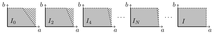
Figure 2. The $(a,b)$-regions $I_{N}$

The next theorem demonstrates that these smaller $(a,b)$-regions are in fact optimal. More concretely, we show that the approximation using $\textnormal{h}_{g}^{(N)}(p)$ fails on the diagonal boundary of $I_{N}$. That is, for $b(a)=(N+2)(1-a)$ with $a\in(1-\frac{1}{2(N+2)},1)$.

Here for simplicity we consider the massless Nelson model (1.7), so that $|||V|||_{\mu}^{2}=O(\log\mu)$.

Theorem 5.1.

Let $N\in 2\mathbb{N}_{0}$ be an even integer, and assume that

$$\varphi=\mathds{1}(\tfrac{1}{2}\mu^{a}\leqslant|p|\leqslant\mu^{a})\varphi\qquad\textnormal{ with }\qquad a\in\bigg{(}1-\frac{1}{2(N+1)}\,,\,1\bigg{)}\ .$$ (5.17)

Then, there exists a constant $\tau=\tau(N)>0$ such that for $t=\tau\mu^{b}$ with $b=(N+2)(1-a)$

$$\liminf_{\mu\to\infty}\Big{\|}\Big{(}e^{-itH}-e^{-it\textnormal{h}_{g}^{(N)}(p)}\Big{)}\varphi\otimes\Omega\Big{\|}>0.$$ (5.18)

Remark 5.1.

To continue the example from Remark 2.3, consider an initial state $\varphi$ satisfying (5.17) with $a=23/24$. Remember that Corollary 2.1 proves

$$\lim_{\mu\to\infty}(\Psi(t)-e^{-it\textnormal{h}_{g}^{(N)}(t)}\varphi\otimes\Omega)=0\quad\text{for all}\quad|t|\ll\min\big{\{}\mu^{1/2}\log(\mu)^{-1},\mu^{(N+2)/24}\big{\}}.$$ (5.19)

By Theorem 5.1, on the other hand, we know that convergence towards $e^{-it\textnormal{h}_{g}^{(N)}(p)}\Psi_{0}$ fails for $t\sim\mu^{(N+2)/24}$. Thus, we can conclude that (5.19) is in fact optimal. Note that in the considered case, we hit the threshold at $N=10$, for which the time scale does not extend further by considering larger values of $N$. The discussion is easily generalized to other choices of $P_{0}=\mu^{a}$.

Proof of Theorem 5.1.

Let $N\in 2\mathbb{N}_{0}$. Throughout this proof we consider the remainder term

$$\mathcal{R}_{N}(p)=\sum_{j\geqslant N+2:j\textnormal{ even }}\alpha_{j}(\mu)|p|^{j}\ \quad\textnormal{on}\quad\tfrac{1}{2}\mu^{a}\leqslant|p|\leqslant\mu^{a}$$ (5.20)

corresponding to the truncation of the series in (5.9) of order $n$. In view of (5.13) we have the following upper bound for $|p|\leqslant\mu^{a}$ with $a<1$ and $\mu>0$ large enough

$$\mathcal{R}_{N}(p)\leqslant C_{1}\mu^{(N+2)(a-1)}\ ,$$ (5.21)

for a constant $C_{1}=C_{1}(N)$. On the other hand, under the assumption $|p|\geqslant\frac{1}{2}\mu^{a}$, it follows from (5.10) that the following lower bounds holds for $\mu>0$ large enough

$$\mathcal{R}_{N}(p)\geqslant\alpha_{N+2}(\mu)|p|^{N+2}\geqslant C_{2}\mu^{(N+2)(a-1)}$$ (5.22)

for a constant $C_{2}\geqslant C(N)\int|k|^{-1}|V(k)|^{2}\mathrm{d}k>0$.

Next, we use these bounds to derive a lower bound for $(e^{-it\textnormal{h}_{g}(p)}-e^{-i\textnormal{h}_{g}^{(N)}(p)})\varphi$. To this end, we invoke Duhamel’s formula twice, that is

$$i\Big{(}1-e^{it\textnormal{h}_{g}(p)}e^{-it\textnormal{h}_{g}^{(N)}(p)}\Big{)}\varphi =\int_{0}^{t}\mathrm{d}te^{is\textnormal{h}_{g}(p)}e^{-is\textnormal{h}_{g}^{(N)}(p)}\Big{(}\textnormal{h}_{g}(p)-\textnormal{h}_{g}^{(N)}(p)\Big{)}\varphi$$

$$=t\Big{(}\textnormal{h}_{g}(p)-\textnormal{h}_{g}^{(N)}(p)\Big{)}\varphi$$

$$\quad-\int_{0}^{t}\mathrm{d}s\int_{0}^{s}\mathrm{d}r\,e^{i(r-s)\textnormal{h}_{g}(p)}e^{-ir\textnormal{h}_{g}^{(N)}(p)}\Big{(}\textnormal{h}_{g}(p)-\textnormal{h}_{g}^{(N)}(p)\Big{)}^{2}\varphi.$$ (5.23)

In view of Proposition 5.1 and 5.9, we have (the ratio $\varepsilon=\mu^{a}/\mu\ll 1$ can be disregarded)

$$\textnormal{h}_{g}(p)-\textnormal{h}^{(N)}_{g}(p)=\mathcal{R}_{N}(p)+O(\mu^{-1}\log(\mu))$$ (5.24)

and thus, using (5.21), (5.22) and $\mu^{-1}\log(\mu)=o(\mu^{(N+2)(1-a)})$ as $\mu\to\infty$, we can estimate

$$\Big{\|}\Big{(}\textnormal{h}_{g}(p)-\textnormal{h}_{g}^{(N)}(p)\Big{)}^{2}\varphi\Big{\|} \leqslant D_{V}\big{(}\mu^{(N+2)(a-1)}\big{)}^{2}$$ (5.25)

$$\Big{\|}\Big{(}\textnormal{h}_{g}(p)-\textnormal{h}_{g}^{(N)}(p)\Big{)}\varphi\Big{\|} \geqslant C_{V}\mu^{(N+2)(a-1)}$$ (5.26)

for suitable constants $D_{V},C_{V}>0$. Choosing $t=\tau\mu^{b}$ with $b=(N+2)(1-a)$ and $\tau^{2}=C_{V}/D_{V}>0$, we arrive at

$$\Big{\|}\Big{(}1-e^{it\textnormal{h}_{g}(p)}e^{-it\textnormal{h}_{g}^{(N)}(p)}\Big{)}\varphi\Big{\|} \geqslant|t|\Big{\|}\Big{(}\textnormal{h}_{g}(p)-\textnormal{h}_{g}^{(N)}(p)\Big{)}\varphi\Big{\|}-\frac{t^{2}}{2}\Big{\|}\Big{(}\textnormal{h}_{g}(p)-\textnormal{h}_{g}^{(N)}(p)\Big{)}^{2}\varphi\Big{\|}$$

$$\geqslant C_{V}\tau-\frac{D_{V}}{2}\tau^{2}=\frac{C_{V}}{2}>0\ .$$ (5.27)

Together with $\limsup_{\mu\to\infty}\|(e^{-itH}-e^{-it\textnormal{h}_{g}(p)})\varphi\otimes\Omega\|=0$ by Theorem 2.2, this proves the claimed statement. ∎

6. Effective dynamics for massive fields

The main goal of this section is to prove Theorem 2.4. To this end, we consider a massive dispersion relation

$$\omega(k)=\sqrt{k^{2}+m^{2}}\$$ (6.1)

with mass term $m\geqslant\mu^{-1}$. In what follows, $\Psi_{0}$ denotes the initial datum satisfying Condition 1 relative to $0<\varepsilon<1/2$, and $V$ is the form factor satisfying Condition 2. We let $\Psi_{\textnormal{eff}}(t)=e^{-it\textnormal{h}_{g}}\varphi\otimes\Omega$ be the effective dynamics, with Hamiltonian $\textnormal{h}_{g}=p^{2}-g(p)$. The generator $g:\mathbb{R}^{3}\rightarrow\mathbb{R}$ is assumed to be bounded and measurable, and shall be chosen below.

The first step is to recall from Section 3 that the following identity holds for all $t\in\mathbb{R}$

$$e^{itH}\Big{(}\Psi(t)-\Psi_{\textnormal{eff}}(t)\Big{)}=\mathcal{I}(t)\Big{(}\mathbb{V}+g(p)\Big{)}\Psi_{0}\ .$$ (6.2)

Recalling our notation ${\bf P}_{\Omega}$ and ${\bf Q}_{\Omega}$ from (3.6), an application of the integration by parts identity yields

$$\mathcal{I}(t){\bf Q}_{\Omega}\mathbb{V} =\mathbb{B}(t)\mathbb{R}\mathbb{V}+\mathcal{I}(t)\mathbb{V}\mathbb{R}\mathbb{V}$$

$$=\mathbb{B}(t)\mathbb{R}\mathbb{V}+\mathcal{I}(t){\bf P}_{\Omega}\mathbb{V}\mathbb{R}\mathbb{V}+\mathcal{I}(t){\bf Q}_{\Omega}\mathbb{V}\mathbb{R}\mathbb{V}\ .$$ (6.3)

Therefore, we combine (6.2) and (6) to find that

$$e^{itH}\Big{(}\Psi(t)-\Psi_{\textnormal{eff}}(t)\Big{)}=\mathbb{B}(t)\mathbb{R}\mathbb{V}\Psi_{0}+\mathcal{I}(t)\Big{(}{\bf P}_{\Omega}\mathbb{V}\mathbb{R}\mathbb{V}\Psi_{0}+g(p)\Psi_{0}\Big{)}+\mathcal{I}(t){\bf Q}_{\Omega}\mathbb{V}\mathbb{R}\mathbb{V}\Psi_{0}\ .$$ (6.4)

The next step is note that the expansion process can be continued, if we now apply the identity (6) to the last term in (6.4) and expand $\mathcal{I}(t){\bf Q}_{\Omega}\mathbb{R}\mathbb{V}\mathbb{R}$ again. This process can be repeated arbitrarily many times. In particular, for $n\in\mathbb{N}$ we find

$$e^{itH}\Big{(} \Psi(t)-\Psi_{\textnormal{eff}}(t)\Big{)}$$ (6.5)

$$=\sum_{1\leqslant j\leqslant n}\mathbb{B}(t)(\mathbb{R}\mathbb{V})^{j}\Psi_{0}+\mathcal{I}(t)\bigg{(}\sum_{\begin{subarray}{c}1\leqslant j\leqslant n\\ j\textnormal{ odd}\end{subarray}}{\bf P}_{\Omega}\mathbb{V}(\mathbb{R}\mathbb{V})^{j}\Psi_{0}+g(p)\Psi_{0}\bigg{)}+\mathcal{I}(t){\bf Q}_{\Omega}\mathbb{V}(\mathbb{R}\mathbb{V})^{n}\Psi_{0}\ ,$$

where we have used the fact that for any even $j\in\mathbb{N}:$ ${\bf P}_{\Omega}\mathbb{V}(\mathbb{R}\mathbb{V})^{j}{\bf P}_{\Omega}=0$.

In the remainder of the section, we show that one can choose a generator $g(p)=g_{n}(p)$ such that the middle term in (6.5) vanishes. Every other term can be regarded as an error term, with precise estimates derived in Section 7. In Section 6.3, the results are combined to prove Theorem 2.4.

6.1. Choosing the generator

Our present goal is to prove that by choosing $g=g_{n}$ as in Definition 2.3, the middle term of (6.5) cancels exactly. This is the content of Lemma 6.1 stated below.

To this end, let us recall the following notation for a special class of collection of sequences $\sigma$ of length $j\in\mathbb{N}$.

$$\Sigma_{0}(j) =\textstyle\{\sigma\in\{+1,-1\}^{j}\ :\ \sum_{i=1}^{\ell}\sigma(i)\geqslant 1\ \forall\ell\leqslant j-1\ \ \textnormal{and}\ \ \sum_{i=1}^{j}\sigma(i)=0\}\ .$$ (6.6)

Next, we introduce auxiliary functions that will help us navigate the proof of the upcoming Lemma. More precisely, let $n\in\mathbb{N}$ and $|p|<\frac{1}{2}\mu$. We define $F_{n}(p,\cdot):(0,\infty)\rightarrow(0,\infty)$ as

$$F_{n}(p,x) :=\sum_{\begin{subarray}{c}j=2\\ j\textnormal{ even }\end{subarray}}^{n+1}\sum_{\sigma\in\Sigma_{0}(j)}F_{j}^{\sigma}(p,x)$$ (6.7)

$$F^{\sigma}_{j}(p,x) :=\mu^{j/2}\int_{\mathbb{R}^{3j}}\mathrm{d}k_{1}\cdots\mathrm{d}k_{j}V(k_{1})\cdots V(k_{j})\,\langle\Omega,b_{k_{j}}^{\#_{\sigma(j)}}\ldots b_{k_{1}}^{\#_{\sigma(1)}}\Omega\rangle$$

$$\qquad\times\prod_{\ell=1}^{j-1}\bigg{(}\mu\sum_{i=1}^{\ell}\sigma(i)\omega(k_{i})+\Big{(}p-\sum_{i=1}^{\ell}\sigma(i)k_{i}\Big{)}^{2}-p^{2}+x\bigg{)}^{-1}\ .$$ (6.8)

In particular, we may re-phrase the definition of $g_{n}(p)$ given in Definition 2.3 in terms as solutions of the fixed point equation

$$g_{n}(p)=F_{n}(p,g_{n}(p))$$ (6.9)

for all $|p|<\frac{1}{2}\mu$.

Lemma 6.1.

Let $n\in\mathbb{N}$ and let $g=g_{n}$ be as in Definition 2.3. Then, it holds that

$$\sum_{\begin{subarray}{c}1\leqslant j\leqslant n\\ j\textnormal{ odd}\end{subarray}}{\bf P}_{\Omega}\mathbb{V}(\mathbb{R}\mathbb{V})^{j}\Psi_{0}=-(g(p)\otimes\mathds{1})\Psi_{0}\ .$$ (6.10)

Proof.

Throughout the proof, we treat $g(p)$ as an arbitrary real-valued, bounded measurable function on $\mathbb{R}^{3}$. The precise choice given by Definition 2.3 will only be made at the end. For transparency, we denote the $g$-dependent resolvent on ${\bf Q}_{\Omega}\mathscr{H}$

$$\mathbb{R}_{g}:=(\textnormal{h}_{g}(p+P)-p^{2}-T)^{-1}$$ (6.11)

We will consider on the Hilbert space $\mathscr{H}=L_{X}^{2}\otimes\mathscr{F}$ the following operator, regarded as a function of $g$:

$$\mathcal{A}_{n}[g]:=\sum_{\begin{subarray}{c}j=2\\ j\textnormal{ even }\end{subarray}}^{n+1}A_{j}[g]\quad\text{with}\quad A_{j}[g]:={\bf P}_{\Omega}\mathbb{V}(\mathbb{R}_{g}{\bf Q}_{\Omega}\mathbb{V})^{j-1}{\bf P}_{\Omega}$$ (6.12)

which coincides with the operator in (6.5) after the change of variables $j\mapsto j-1$.

First, we use the decomposition $\mathbb{V}=\mathbb{V}^{+}+\mathbb{V}^{+}$ into creation and annihilation operators, in each factor of $A_{j}[g]$. The expansion can be represented as a sum over sequences $\sigma\in\Sigma_{0}(j)$ as follows

$$A_{j}[g]=\sum_{\sigma\in\Sigma_{0}(j)}A_{j}^{\sigma}[g],\quad A_{j}^{\sigma}[g]:={\bf P}_{\Omega}\mathbb{V}^{\sigma(j)}\mathbb{R}_{g}\mathbb{V}^{\sigma(j-1)}\cdots\mathbb{R}_{g}\mathbb{V}^{\sigma(1)}{\bf P}_{\Omega}\ .$$ (6.13)

Here, we have dropped the projections ${\bf Q}_{\Omega}$ in (6.12) at the expense of summing over the sequences $\sigma\in\Sigma_{0}(j)$. The summability condition $\sum_{i=1}^{\ell}\sigma(i)\geqslant 1\ \forall\ell\leqslant j-1$ guarantees that $\mathbb{R}_{g}$ acts on states that contain at least one particle.

The next step is to compute the operator $A^{\sigma}_{j}[g]$ using commutation relations between $\mathbb{R}_{g}$ and $e^{-ikX}$ and $b_{k}$ and $b_{k}^{*}$:

$$\mathbb{R}_{g}e^{ik_{i}X}b_{k_{i}} =e^{ik_{i}X}b_{k_{i}}\big{(}\textnormal{h}_{g}(p+P)-(p+k_{i})^{2}-T+\mu\omega(k_{i})\big{)}$$ (6.14)

$$\mathbb{R}_{g}e^{-ik_{i}X}b_{k_{i}}^{*} =e^{-ik_{i}X}b_{k_{i}}^{*}\big{(}\textnormal{h}_{g}(p+P)-(p-k_{i})^{2}-T-\mu\omega(k_{i})\big{)}\ .$$ (6.15)

The idea is to move all the factors $e^{ikX}b_{k}$ and $e^{-ikX}b_{k}^{*}$ to the left of all the resolvents, in the operator (6.13). Once they hit the vacuum projection ${\bf P}_{\Omega}$ on the right, the shifted resolvents are evaluated using $T\Omega=P\Omega=0$. The result is an operator that only acts on the $L_{X}^{2}$ variables, tensored with the monomial $b_{k_{j}}^{\#_{\sigma(j)}}\ldots b_{k_{1}}^{\#_{\sigma(1)}}$. One then takes the vacuum expectation value over such monomial. This calculation yields (here $p=-i\nabla_{X}$ and $\int=\int_{\mathbb{R}^{3j}}\mathrm{d}k_{1}\cdots\mathrm{d}k_{j}$)

$$A_{j}^{\sigma}[g]=\mu^{j/2}\int V(k_{1})\cdots V(k_{j})\prod_{\ell=1}^{j-1}R_{g}^{\sigma(1)\cdots\sigma(\ell)}(p;k_{1},\cdots,k_{\ell})\langle\Omega,b_{k_{j}}^{\#_{\sigma(j)}}\ldots b_{k_{1}}^{\#_{\sigma(1)}}\Omega\rangle\otimes\mathds{1}$$ (6.16)

where we introduce the following operators on $L_{X}^{2}$

$$R_{g}^{\sigma(1)\ldots\sigma(\ell)}(p;k_{1},\ldots,k_{\ell}) =(-1)\textstyle\bigg{(}\mu\sum_{i=1}^{\ell}\sigma(i)\omega(k_{i})+\Big{(}p-\sum_{i=1}^{\ell}\sigma(i)k_{i}\Big{)}^{2}-p^{2}+g(p)\bigg{)}^{-1}$$ (6.17)

Finally, in terms of the auxiliary functions introduced in (6.7) we identify that $A_{j}^{\sigma}[g]\Psi_{0}=(-1)^{j-1}F_{j}^{\sigma}(p,g(p))\otimes\mathds{1}\Psi_{0}$ where the right hand side is evaluated on the operator $p=-i\nabla_{X}$ in the spectral subspace $\mathds{1}(|p|\leqslant\varepsilon\mu)$. We sum over all sequences $\sigma\in\Sigma_{0}(j)$ and all even $2\leqslant j\leqslant n+1$ to obtain

$$\mathcal{A}_{n}[g]\Psi_{0}=\sum_{\begin{subarray}{c}j=2\\ j\textnormal{ even }\end{subarray}}^{n+1}A_{j}^{\sigma}[g]\Psi_{0}=-\sum_{\begin{subarray}{c}j=2\\ j\textnormal{ even }\end{subarray}}^{n+1}F_{j}^{\sigma}(p,g(p))\otimes\mathds{1}\,\Psi_{0}=-F_{n}(p,g(p))\otimes\mathds{1}\,\Psi_{0}\ .$$ (6.18)

Therefore, by choosing $g=g_{n}$ as in Definition 2.3 we see that $\mathcal{A}_{n}[g_{n}]\Psi_{0}=-g_{n}(p)\otimes\mathds{1}\Psi_{0}$. This finishes the proof. ∎

6.2. Estimate for $(\mathbb{R}\mathbb{V})^{n}\Psi_{0}$

In this subsection, we state some estimates that we will need in order to control the expansion (6.5). The main challenge is to estimate terms of the form

$$\underbrace{\mathbb{R}\mathbb{V}^{\#}\cdots\mathbb{R}\mathbb{V}^{\#}}_{n\textnormal{ times }}(\varphi\otimes\Omega)\ .$$ (6.19)

Here, $\mathbb{V}^{\#}$ can be either a creation $\mathbb{V}^{+}$ or annihilation $\mathbb{V}^{-}$ operator (see (4.2) for a definition) and $\mathbb{R}$ is the resolvent operator, introduced in Definition 3.2. It is crucial to observe that the presence of the projections ${\bf Q}_{\Omega}$ in the definition of $\mathbb{R}$ guarantees that the states (6.19) are either zero, or contain at least one particle.

In this regard, our most relevant result is Proposition 6.1 stated below. In order to formulate it, we introduce some some notation that encodes the structure of the states (6.19). Let us consider the set of sequences of length $n$, taking values on $\{+1,-1\}$, and whose all partial sums are bounded below by one. That is,

$$\Sigma(n):=\textstyle\{\sigma\in\{+1,-1\}^{n}\ :\ \sum_{i=1}^{j}\sigma(i)\geqslant 1\ \forall j=1,\ldots,n\}\ ,\qquad n\in\mathbb{N}\ .$$ (6.20)

Contrary to $\Sigma_{0}(n)$, the set of sequences in $\Sigma(n)$ do not drop to zero at the last entry.

The proof of the following proposition is rather involved and will be postponed to Section 7. We remind the reader that we assume $m\geqslant\mu^{-1}$. Here, we employ the notation $\mathbb{V}^{+1}\equiv\mathbb{V}^{+}$ and $\mathbb{V}^{-1}\equiv\mathbb{V}^{-}$, and $n_{\pm}\equiv|\{i:\sigma(i)=\pm 1\}|$ whenever $\sigma$ is known from context.

Proposition 6.1.

Let $n\geqslant 2$. Then, there exists a constant $C>0$ such that for all sequences $\sigma\in\Sigma(n)$

$$\bigg{\|}\prod_{i=1}^{n}(\mathbb{R}\mathbb{V}^{\sigma(i)})(\varphi\otimes\Omega)\bigg{\|}_{\mathscr{H}}\leqslant\frac{C^{n}}{\mu^{n/2}}\sqrt{(n_{+}-n_{-})!}\bigg{(}\frac{1}{m}\bigg{)}^{n_{-}}|||V|||_{\mu}^{n_{+}}\|V\|_{L^{2}}^{n_{-}}\$$ (6.21)

for all $\mu>0$ large enough.

Remark 6.1.

Two comments are in order

1. The summability conditions implies $n_{+}-n_{-}\geqslant 1$. On the other hand, $n=n_{-}+n_{+}$. Consequently, $2n_{-}\leqslant n-1$ or equivalently $n_{-}\leqslant\lfloor\frac{n-1}{2}\rfloor$ represents the worst possible scenario, regarding the growth with respect to $m$. In particular, we obtain the following bound that is uniform over all $\sigma\in\Sigma(n)$

   $$\bigg{\|}\prod_{i=1}^{n}(\mathbb{R}\mathbb{V}^{\sigma(i)})(\varphi\otimes\Omega)\bigg{\|}_{\mathscr{H}}\leqslant\frac{C^{n}\sqrt{n!}}{\mu^{n/2}}\bigg{(}\frac{1}{m}\bigg{)}^{\lfloor\frac{n-1}{2}\rfloor}|||V|||_{\mu}^{n}\ .$$ (6.22)

   where we used $\|V\|_{L^{2}}\leqslant C\|V\|_{\mu}$. This bound, although not optimal with respect to $n\in\mathbb{N}$, will be useful in the proof of the main theorem.

2. Consider a $\mu$-dependent mass term $m=\mu^{-\delta}$ where $\delta\in(0,1)$ and let $n$ be odd. Then, the right hand side of (6.22) is of order $\mu^{-\frac{1}{2}(n(1-\delta)-\delta)}$. In particular, the rate gets better with the order of iteration $n\geqslant 1$, but this growth is modulated by $\delta$, i.e. the size of the mass term. Further, the case is $m=\mu^{-1}$ is critical: our bound on the rate of convergence does not improve with $n\geqslant 1$ but rather stagnates.

6.3. Proof of Theorem 2.4

We now have all the necessary ingredients to prove our main approximation result for massive fields.

Proof of Theorem 2.4.

Let $\Psi_{\textnormal{eff}}^{(n)}(t)=e^{-it\textnormal{h}_{g_{n}}}\varphi\otimes\Omega$ where the generator $g_{n}$ is chosen as in Definition 2.3. It follows immediately from (6.5), Lemma 6.1 and $\|\mathbb{B}(t)\|\leqslant 2$ that

$$\|\Psi^{(n)}_{\textnormal{eff}}(t)-\Psi(t)\|\leqslant 2\sum_{1\leqslant j\leqslant n}\|(\mathbb{R}\mathbb{V})^{j}\Psi_{0}\|+\|\mathcal{I}(t){\bf Q}_{\Omega}\mathbb{V}(\mathbb{R}\mathbb{V})^{n}\Psi_{0}\|\ .$$ (6.23)

Next, let us note that since $n$ is odd, the state $\Psi_{n}:={\bf Q}\mathbb{V}(\mathbb{R}\mathbb{V})^{n}\Psi_{0}$ has a trivial one-particle sector, and a non-trivial two-particle sector. In particular, ${\bf P}_{\Omega}\mathbb{V}\mathbb{R}\Psi_{n}=0$. Thus, integrating by parts one more time (i.e. apply (6)) leads to

$$\mathcal{I}(t)\Psi_{n} =\mathbb{B}(t)\mathbb{R}\Psi_{n}+\mathcal{I}(t)\mathbb{V}\mathbb{R}\Psi_{n}=\mathbb{B}(t)\mathbb{R}\Psi_{n}+\mathcal{I}(t){\bf Q}_{\Omega}\mathbb{V}\mathbb{R}\Psi_{n}$$ (6.24)

Below we will use this identity in the case $\mu^{-1}\leqslant m\leqslant\mu^{-1/2}|||V|||_{\mu}$, which we call the small mass case. Conversely, in the opposite large mass case $m\geqslant\mu^{-1/2}|||V|||_{\mu}$, it is favourable to apply the integration by parts formula one more time, that is

$$\mathcal{I}(t)\Psi_{n} =\mathbb{B}(t)\mathbb{R}\Psi_{n}+\mathbb{B}(t)\mathbb{R}\mathbb{V}\mathbb{R}\Psi_{n}+\mathcal{I}(t)\mathbb{V}\mathbb{R}\mathbb{V}\mathbb{R}\Psi_{n}\ .$$ (6.25)

For the remainder estimates, note that in the first case, the relevant state is $\mathbb{R}\Psi_{n}=(\mathbb{R}\mathbb{V})^{n+1}\Psi_{0}$ which contains at most $n+1$ particles, an even number. In the second case, the relevant state is $\mathbb{R}\mathbb{V}\mathbb{R}\Psi_{n}=(\mathbb{R}\mathbb{V})^{n+2}\Psi_{0}$ which contains at most $n+2$ particles, an odd number. This on its turn implies that the least integer bracket in the estimate (6.22) takes different values and thus makes the dependence on the mass term different.

The small mass case. An application of (6.23), (6.24) and (6.22) yields

$$\|\Psi^{(n)}_{\textnormal{eff}}(t)-\Psi(t)\| \leqslant 2\sum_{j=1}^{n+1}\|(\mathbb{R}\mathbb{V})^{j}\Psi_{0}\|+\,|t|\,\mu^{1/2}\,\|V\|_{L^{2}}(n+2)^{\frac{1}{2}}\|(\mathbb{R}\mathbb{V})^{n+1}\Psi_{0}\|$$ (6.26)

$$\leqslant\sum_{j=1}^{n+1}\frac{C^{j}\sqrt{j!}}{\mu^{j/2}}\bigg{(}\frac{1}{m}\bigg{)}^{\lfloor\frac{j-1}{2}\rfloor}|||V|||_{\mu}^{j}+\,|t|\,\sqrt{(n\!+\!2)!}\,\frac{C^{n+1}}{\mu^{\frac{n}{2}}}\bigg{(}\frac{1}{m}\bigg{)}^{\frac{n-1}{2}}|||V|||_{\mu}^{n+1}$$

where in the last line we have evaluated $\lfloor\frac{n}{2}\rfloor=\frac{n-1}{2}$ for $n$ odd. The above bound records the dependence of the estimates with respect to $n\in\mathbb{N}$. Let us now simplify it. First, without loss of generality we assume $\mu^{-1/2}|||V|||_{\mu}\leqslant 1$ (otherwise the bound in Theorem 2.4 holds trivially). Next, for the $t$-independent error we estimate the summands using $C^{j}\sqrt{j!}\leqslant C^{n+1}\sqrt{(n+1)!}$ as well as the following inequalities (recall $n$ is odd):

$$\sum_{j=1}^{n+1}\frac{|||V|||_{\mu}^{j}}{\mu^{j/2}}\bigg{(}\frac{1}{m}\bigg{)}^{\lfloor\frac{j-1}{2}\rfloor} =\sum_{\begin{subarray}{c}j=1\\ j\,\text{odd}\end{subarray}}^{n}\frac{|||V|||_{\mu}^{j}}{\mu^{j/2}}\bigg{(}\frac{1}{m}\bigg{)}^{\frac{j-1}{2}}+\sum_{\begin{subarray}{c}j=2\\ j\,\text{even }\end{subarray}}^{n+1}\frac{|||V|||_{\mu}^{j}}{\mu^{j/2}}\bigg{(}\frac{1}{m}\bigg{)}^{\frac{j-2}{2}}$$

$$=\sum_{\begin{subarray}{c}j=1\\ j\,\text{odd}\end{subarray}}^{n}\frac{|||V|||_{\mu}^{j}}{\mu^{j/2}}\bigg{(}\frac{1}{m}\bigg{)}^{\frac{j-1}{2}}+\frac{|||V|||_{\mu}}{\mu^{1/2}}\sum_{\begin{subarray}{c}j=1\\ j\,\text{odd }\end{subarray}}^{n}\frac{|||V|||_{\mu}^{j}}{\mu^{j/2}}\bigg{(}\frac{1}{m}\bigg{)}^{\frac{j-1}{2}}$$

$$=\bigg{(}1+\frac{|||V|||_{\mu}}{\mu^{1/2}}\bigg{)}\sqrt{m}\sum_{\begin{subarray}{c}j=1\\ j\,\text{odd}\end{subarray}}^{n}\frac{|||V|||_{\mu}^{j}}{\mu^{j/2}}\bigg{(}\frac{1}{m}\bigg{)}^{\frac{j}{2}}$$

$$\leqslant 2n\bigg{(}\frac{|||V|||_{\mu}}{\mu^{1/2}}+\frac{|||V|||_{\mu}^{n}}{\mu^{n/2}}\bigg{(}\frac{1}{m}\bigg{)}^{\frac{n-1}{2}}\bigg{)}\ .$$ (6.27)

In the first line, we evaluated even and odd terms; in the second line we shifted the second sum $j\to j+1$ and in third line we grouped terms. In the last line we used $\mu^{-1/2}|||V|||_{\mu}\leqslant 1$ and elementary geometric series estimates. This gives (here we absorb $n\leqslant C^{n}$)

$$\|\Psi^{(n)}_{\textnormal{eff}}(t)-\Psi(t)\| \ \leqslant\ C^{n}\,\sqrt{n!}\,\bigg{(}\ \bigg{[}\frac{|||V|||_{\mu}}{\mu^{1/2}}\,+\,\frac{|||V|||_{\mu}^{n}}{\mu^{n/2}}\bigg{(}\frac{1}{m}\bigg{)}^{\frac{n-1}{2}}\bigg{]}\ +\ \frac{|t|}{\mu^{1/2}}\frac{|||V|||_{\mu}^{n+1}}{(\mu m)^{\frac{n-1}{2}}}\ \bigg{)}$$ (6.28)

The large mass case. An application of (6.23), (6.25) and (6.22) yields

$$\|\Psi^{(n)}_{\textnormal{eff}}(t)-\Psi(t)\| \leqslant 2\sum_{1\leqslant j\leqslant n+2}\|(\mathbb{R}\mathbb{V})^{j}\Psi_{0}\|+\,|t|\,\mu^{\frac{1}{2}}\,\|V\|_{L^{2}}(n+3)^{\frac{1}{2}}\|(\mathbb{R}\mathbb{V})^{n+2}\Psi_{0}\|$$ (6.29)

$$\leqslant\sum_{1\leqslant j\leqslant n+2}\frac{C^{j}\sqrt{j!}}{\mu^{j/2}}\bigg{(}\frac{1}{m}\bigg{)}^{\lfloor\frac{j-1}{2}\rfloor}|||V|||_{\mu}^{j}+\,|t|\,\frac{C^{n+2}\sqrt{(n\!+\!3)!}}{\mu^{(n+1)/2}}\bigg{(}\frac{1}{m}\bigg{)}^{\frac{n+1}{2}}|||V|||_{\mu}^{n+2}$$

where in the last line we have evaluated $\lfloor\frac{n+1}{2}\rfloor=\frac{n+1}{2}$ for $n$ odd. In order to simplify the $t$-independent term we use $C^{j}\sqrt{j!}\leqslant C^{n}\sqrt{n!}$ for the summands. Additionally, we use the calculation (6.27) and include an additional term to the sum to find

$$\sum_{j=1}^{n+2}\frac{|||V|||_{\mu}^{j}}{\mu^{j/2}}\bigg{(}\frac{1}{m}\bigg{)}^{\lfloor\frac{j-1}{2}\rfloor}\leqslant 2(n+1)\bigg{(}\frac{|||V|||_{\mu}}{\mu^{1/2}}+\frac{|||V|||_{\mu}^{n+2}}{\mu^{\frac{n+2}{2}}}\bigg{(}\frac{1}{m}\bigg{)}^{\frac{n+1}{2}}\bigg{)}\leqslant Cn\frac{|||V|||_{\mu}}{\mu^{1/2}}$$ (6.30)

where in the last inequality we use that for all $k\in\mathbb{N}$ in the large mass regime:

$$\frac{|||V|||_{\mu}^{k}}{\mu^{\frac{k}{2}}}\bigg{(}\frac{1}{m}\bigg{)}^{\frac{k-1}{2}}\ =\ \bigg{(}\frac{|||V|||_{\mu}}{\mu^{1/2}m}\bigg{)}^{\frac{k-1}{2}}\bigg{(}\frac{|||V|||_{\mu}}{\mu^{1/2}}\bigg{)}^{\frac{k+1}{2}}\ \leqslant\ \frac{|||V|||_{\mu}}{\mu^{1/2}}$$ (6.31)

Thus, we arrive at (again, we absorb powers of $n$ in $C^{n}$):

$$\|\Psi^{(n)}_{\textnormal{eff}}(t)-\Psi(t)\| \ \leqslant\ C^{n}\,\sqrt{n!}\,\bigg{(}\frac{|||V|||_{\mu}}{\mu^{\frac{1}{2}}}+\frac{|t|}{\mu^{1/2}}\frac{|||V|||_{\mu}^{n+1}}{(\mu m)^{\frac{n-1}{2}}}\frac{|||V|||_{\mu}}{\mu^{\frac{1}{2}}m}\bigg{)}\ .$$ (6.32)

The proof of the theorem is finished once we combine (6.32) and (6.28). ∎

7. Resolvent estimates

The main goal of this section is to give a proof of Proposition 6.1, stated in Section 6.2, which allows us to control the norm of states of the form (6.19) in the case of massive fields. Thus, we assume throughout this section that the dispersion relation is given by

$$\omega(k)=\sqrt{k^{2}+m^{2}}$$ (7.1)

with $m\geqslant\mu^{-1}$. The generator is taken as in Definition 2.3, but the results in this Section apply to any non-negative bounded measurable function $g(p)\geqslant 0$.

Throughout this section, the parameter $0\leqslant\varepsilon<1/2$ is fixed, and $V$ is the form factor satisfying Condition 2.

The organization of this section is as follows: In Subsection 7.1 we introduce relevant resolvent functions. In Subsection 7.2 we give an example of an estimate for a state (6.19) consisting of only $\mathbb{V}^{+}$. Finally, in Subsection 7.3 we turn to the proof of Proposition 6.1.

7.1. Resolvents

Let us generalize the resolvents (4.20) and (4.21) that naturally emerged in the proof of Theorem 2.2. To this end, let $n\geqslant 1$ and $k_{1},\cdots,k_{n}\in\mathbb{R}^{3}$. We denote ${\bm{k}}_{n}\equiv(k_{1},\ldots,k_{n})\in\mathbb{R}^{3n}$. For $p\in\mathbb{R}^{3}$, we introduce the following notations

$$\textstyle R_{p}({\bm{k}}_{n}):=(-1)\bigg{(}\mu\sum_{i=1}^{n}\omega(k_{i})+(p-\sum_{i=1}^{n}k_{i})^{2}-p^{2}+g(p)\bigg{)}^{-1}$$ (7.2)

$$\textstyle R_{p}({\bm{k}}_{n}\big{|}k):=(-1)\bigg{(}\mu\sum_{i=1}^{n}\omega(k_{i})-\mu\,\omega(k)+(p-\sum_{i=1}^{n}k_{i}+k)^{2}-p^{2}+g(p)\bigg{)}^{-1}$$ (7.3)

Note that both $R_{p}({\bm{k}}_{n})$ and $R_{p}({\bm{k}}_{n}|k)$ are symmetric with respect to the permutation of the variables $k_{1},\cdots,k_{n}$. We often refer to $R_{p}({\bm{k}}_{n}|k)$ as the contracted resolvent. In particular, we observe that for all $1\leqslant i\leqslant n$ there holds

$$R_{p}({\bm{k}}_{n}|k_{i})=R_{p}({\bm{k}}_{n}^{(i)})$$ (7.4)

where ${\bm{k}}_{n}^{(i)}\equiv(k_{1},\ldots,k_{i-1},k_{i+1},\ldots,k_{n})\in\mathbb{R}^{3(n-1)}$.

The following estimates will be crucial in our analysis. We remind the reader of the notation $\omega_{\mu}(k)=\omega(k)+\mu^{-1}$ and $|||V|||_{\mu}\equiv\|\omega_{\mu}^{-1}V\|_{L^{2}}$.

Lemma 7.1.

Let $n\geqslant 1$. Then, the following is true for all $|p|\leqslant\varepsilon\mu$ and all $1\leqslant i\leqslant n$:

1. There exists a constant $C>0$ such that for all ${\bm{k}}_{n}\in\mathbb{R}^{3n}$

   $$|R_{p}({\bm{k}}_{n})|\leqslant\frac{C}{\mu\omega_{\mu}(k_{i})}$$ (7.5)

2. If $n\geqslant 2$, then also for all ${\bm{k}}_{n}\in\mathbb{R}^{3n}$

   $$|R_{p}({\bm{k}}_{n}|k_{i})|\leqslant\frac{C}{(n-1)m\mu}\ .$$ (7.6)

Proof.

(1) The denominator on the right hand side of (7.2) can be bounded below using $p\cdot k\leqslant\varepsilon\mu|k|$ and $g(p)\geqslant$ . We find that

$$\textstyle\mu\sum_{j=1}^{n}\omega(k_{j})+(p-\sum_{j=1}^{n}k_{j})^{2}-p^{2}+g(p) =\textstyle\sum_{j=1}^{n}\big{(}\mu\,\omega(k_{j})-2p\cdot k_{j}\big{)}+(\sum_{j=1}^{n}k_{j})^{2}+g(p)$$

$$\textstyle\geqslant C\sum_{j=1}^{n}\mu\omega(k_{j})\ .$$ (7.7)

Next, note that we can use the bound $m\geqslant\mu^{-1}$ and obtain that for constants $C_{1}$ and $C_{2}$

$$C_{1}\omega_{\mu}(k)\leqslant\omega(k)\leqslant C_{2}\omega_{\mu}(k)\ .$$ (7.8)

Note also that (7.7) implies $R_{p}({\bm{k}})<0$. This finishes the proof of the first item, after we use the trivial bound $\sum_{j=1}^{n}\omega_{\mu}(k_{j})\geqslant\omega_{\mu}(k_{i})$. The proof of item (2) is analogous. Here we use the contraction identity (7.4), and use the alternative lower bound $\omega(k_{j})\geqslant m$. ∎

Remark 7.1 (Heuristics).

We are interested in the regime for which $\omega_{\mu}^{-1}V\in L^{2}$ grows much slower than $\mu>0$ (for instance, logarithmically as in the Nelson model). Consequently, the generic bound that we use for the resolvent function is of the form (here $n=1$)

$$\mu^{1/2}\|R_{p}(k)V(k)\|_{L^{2}}\leqslant\frac{C}{\mu^{1/2}}|||V|||_{\mu}$$

uniformly in $|p|\leqslant\varepsilon\mu.$ Thus, up to the $|||V|||_{\mu}$ norm, this estimate extracts a full factor $\mu^{-1/2}$. Hence, we refer to resolvent functions as good resolvents.

On the other hand for the contracted resolvents we use the generic bound (here $n=2$) for some function $\psi\in L^{2}(\mathbb{R}^{6})$

$$\mu^{1/2}\|R_{p}(k_{1},k_{2}\big{|}k_{1})V(k_{1})\psi(k_{1},k_{2})\|_{L^{2}}\leqslant\frac{C}{\mu^{1/2}m}\|V\|_{L^{2}}\|\psi\|_{L^{2}}$$

which is only able to extract the possibly larger factor $\mu^{-1/2}m^{-1}$, uniformly in $|p|\leqslant\varepsilon\mu.$ Hence, we refer to these as bad resolvents.

Remark 7.2 (Operator calculus).

The resolvent functions $R_{p}({\bm{k}}_{n})$ define bounded operators on the spectral subspace $\mathds{1}(|p|\leqslant\varepsilon\mu)L_{X}^{2}$ via spectral calculus of $p=-i\nabla_{X}$, which we extend by zero to $L_{X}^{2}$. Unless confusion arises we also denote these operators by $R_{p}({\bm{k}}_{n})$. In particular, the estimates (7.5) are translated into operator norm estimates.

Remark 7.3.

The bounds (7.5) also apply in the massless case $m=0$ provided the generator satisfies the lower bound $g(p)\geqslant C$. This only has the effect of changing the value of the constant in Lemma 7.1, and we will use this observation in Appendix A.

7.2. An example

Before we turn to the estimates of a general product state (6.19), let us warm up with an example that only contains good resolvents. This state arises as the case where only $\mathbb{V}^{+}$ operators are considered, as no contractions are present.

For $n\geqslant 1$ one can calculate the following representation for the $n$-body state using commutation relations

$$(\mathbb{R}\mathbb{V}^{+}\cdots\mathbb{R}\mathbb{V}^{+})(\varphi\otimes\Omega) =\mu^{\frac{n}{2}}\int_{\mathbb{R}^{3k}}e^{-i\sum_{i}k_{i}\cdot X}\prod_{i=1}^{n}V(k_{i})R_{p}({\bm{k}}_{i})\varphi\otimes b_{k_{n}}^{*}\cdots b_{k_{1}}^{*}\Omega\mathrm{d}k_{1}\cdots\mathrm{d}k_{n}\ .$$ (7.9)

In particular, thanks to Lemma 7.1 and the number estimate (4.11) we find that

$$\|(\mathbb{R}\mathbb{V}^{+}\cdots\mathbb{R}\mathbb{V}^{+})(\varphi\otimes\Omega)\|_{\mathscr{H}}^{2} \ \leqslant\ n!\mu^{n}\,\int_{\mathbb{R}^{3(n+1)}}\prod_{i=1}^{n}|V(k_{i})|^{2}\|R_{p}({\bm{k}}_{i})\varphi\|_{L_{X}^{2}}^{2}\mathrm{d}k_{1}\cdots\mathrm{d}k_{n}$$

$$\ \leqslant\ \frac{C^{n}n!}{\mu^{n}}|||V|||_{\mu}^{2n}\ .$$ (7.10)

Here, $C>0$ is a constant independent of $n$.

7.3. The general case

In the previous example, there were only good resolvents because only creation operators $\mathbb{V}^{+}$ were used. When annihilation operators $\mathbb{V}^{-}$ are present, one needs to be more careful because bad resolvents show up: these are of the form $R_{p}({\bm{k}}_{n}\big{|}k)$. For these, we carry on the contractions between creation- and annihilation- operators to estimate them. We now study this process.

In what follows, we denote $\overline{B}_{\varepsilon\mu}\equiv\{p\in\mathbb{R}^{3}:|p|\leqslant\varepsilon\mu\}$. Our first step is to introduce an appropriate class of functions with a relevant norm. Namely, for $n\in\mathbb{N}$ we consider

$$\mathcal{M}\in L^{2}L^{\infty}(\mathbb{R}^{dn}\times\overline{B}_{\varepsilon\mu})\equiv L^{2}\big{(}\mathbb{R}^{3n};L^{\infty}(\overline{B}_{\varepsilon\mu})\big{)}$$ (7.11)

which we equip with the norm

$$\|\mathcal{M}\|_{L^{2}L^{\infty}}:=\bigg{(}\int_{\mathbb{R}^{3}}\Big{(}\sup_{|p|\leqslant\varepsilon\mu}|\mathcal{M}({\bm{k}}_{n},p)|\Big{)}^{2}\mathrm{d}k\bigg{)}^{1/2}\ .$$ (7.12)

Analogously as in Remark 7.2, these functions induce bounded operators $\mathcal{M}({\bm{k}}_{n},p)$ on $L_{X}^{2}$.

Example. Up to irrelevant factors, these functions should be regarded as the coefficients of the product states (6.19). For instance, in the previous example we have

$$(\mathbb{R}\mathbb{V}^{+}\cdots\mathbb{R}\mathbb{V}^{+})(\varphi\otimes\Omega)=\int_{\mathbb{R}^{3k}}e^{-i\sum_{i}k_{i}\cdot X}\mathcal{M}_{n}({\bm{k}}_{n},p)\varphi\otimes b_{k_{n}}^{*}\cdots b_{k_{1}}^{*}\Omega\mathrm{d}k_{1}\cdots\mathrm{d}k_{n}\ .$$ (7.13)

with $\mathcal{M}_{n}({\bm{k}}_{n},p):=\mu^{\frac{n}{2}}\prod_{i=1}^{n}V(k_{i})R_{p}({\bm{k}}_{i})$.

The specific example given above can be readily generalized in the following sense.

Definition 7.1.

Let $n\in\mathbb{N}$. Then, to any $\mathcal{M}\in L^{2}L^{\infty}(\mathbb{R}^{dn}\times\overline{B}_{\varepsilon\mu})$ we associate the $n$-particle state

$$\Phi_{\mathcal{M}}:=\int_{\mathbb{R}^{3k}}e^{-i\sum_{i}k_{i}\cdot X}\mathcal{M}({\bm{k}}_{n},p)\varphi\otimes b_{k_{n}}^{*}\cdots b_{k_{1}}^{*}\Omega\mathrm{d}k_{1}\cdots\mathrm{d}k_{n}\ .$$ (7.14)

Remark 7.4.

For any $\mathcal{M}\in L^{2}L^{\infty}(\mathbb{R}^{dn}\times\overline{B}_{\varepsilon\mu})$ the number estimate (4.11) shows that

$$\|\Phi_{\mathcal{M}}\|_{\mathscr{H}}\leqslant\sqrt{n!}\,\|\mathcal{M}\|_{L^{2}L^{\infty}}\ .$$ (7.15)

The bound (7.15) motivates the introduction of the space $L^{2}L^{\infty}(\mathbb{R}^{dn}\times\overline{B}_{\varepsilon\mu})$. Let us also mention here that we have included the pre-factor $(-1)^{n}e^{-i\sum k_{i}\cdot X}$ only for convenience.

Our next goal is to study the action of $\mathbb{R}\mathbb{V}^{+}$ and $\mathbb{R}\mathbb{V}^{-}$ on states $\Phi_{\mathcal{M}}$. This calculation is recorded in the following lemma, which is a straightforward consequence of the definitions of $\mathbb{V}^{+}$, $\mathbb{V}^{-}$, $\mathbb{R}$ and the commutation relations.

Lemma 7.2.

Let $\mathcal{M}\in L^{2}L^{\infty}(\mathbb{R}^{dn}\times\overline{B}_{\varepsilon\mu})$ and $\Phi_{\mathcal{M}}$ be as in Definition 7.1. Then,

1. For all $n\geqslant 1$ it holds that $\mathbb{R}\mathbb{V}^{+}\Phi_{\mathcal{M}}=\Phi_{\mathcal{M}^{+}}$ where

   $$\mathcal{M}_{+}({\bm{k}}_{n+1},p):=\mu^{1/2}V(k_{n+1})R_{p}({\bm{k}}_{n+1})\mathcal{M}({\bm{k}}_{n},p)\ .$$ (7.16)

2. For all $n\geqslant 2$ it holds that $\mathbb{R}\mathbb{V}^{-}\Phi_{\mathcal{M}}=\Phi_{\mathcal{M}^{-}}$ where

   $$\mathcal{M}_{-}({\bm{k}}_{n-1},p):=\mu^{1/2}\sum_{i=1}^{n}\int_{\mathbb{R}^{3}}V(k_{n})R_{p}({\bm{k}}_{n-1})\mathcal{M}(\pi_{i}{\bm{k}}_{n},p)\mathrm{d}k_{n}\ ,$$ (7.17)

   where we denote ${\bm{k}}_{n}\equiv({\bm{k}}_{n-1},k_{n})\in\mathbb{R}^{dn}$ and $\pi_{i}\in S_{n}$ is the transposition that changes $k_{i}$ and $k_{n}$, i.e. $\pi_{i}{\bm{k}}_{n}=(k_{1}\cdots k_{n}\cdots k_{i})$.

Remark 7.5.

Using the notation of Lemma 7.2, we find that thanks to the resolvent estimates of Lemma 7.1 the following upper bounds hold: for $n\geqslant 1$

$$\|\mathcal{M}_{+}\|_{L^{2}L^{\infty}}\leqslant\frac{C}{\mu^{1/2}}|||V|||_{\mu}\|\mathcal{M}\|_{L^{2}L^{\infty}}$$ (7.18)

and for $n\geqslant 2$ (here we use $n/(n-1)\leqslant 2$)

$$\|\mathcal{M}_{-}\|_{L^{2}L^{\infty}}\leqslant\frac{C}{\mu^{1/2}m}\|V\|_{L^{2}}\|\mathcal{M}\|_{L^{2}L^{\infty}}\ ,$$ (7.19)

where for the $\mathcal{M}_{-}$ bound we made use of the Cauchy-Schwarz inequality.

We now have all the ingredients that we need to estimate the general product states (6.19), i.e. we turn to the proof of Proposition 6.1. Let us remind the reader of the notation

$$\Sigma(n)=\textstyle\{\sigma\in\{+1,-1\}^{n}\ :\ \sum_{i=1}^{j}\sigma(i)\geqslant 1\ \forall j=1,\ldots,n\}\ ,\qquad n\in\mathbb{N}\ .$$ (7.20)

as well as $\mathbb{V}^{+1}\equiv\mathbb{V}^{+}$, $\mathbb{V}^{-1}\equiv\mathbb{V}^{-}$ and when $\sigma$ is known from context $n_{\pm}\equiv|\{i:\sigma(i)=\pm 1\}|$.

Proof of Proposition 6.1.

Note that for all $\sigma\in\Sigma(n)$ it holds that $\sigma(1)=\sigma(2)=+1$. Then, let us start the proof by considering the following two-body state (see e.g. Definition 7.1)

$$\mathbb{R}\mathbb{V}^{+}\mathbb{R}\mathbb{V}^{+}(\varphi\otimes\Omega)=\Phi_{\mathcal{M}_{2}}\qquad\textnormal{with}\qquad\mathcal{M}_{2}({\bm{k}}_{2},p)=\mu V(k_{1})V(k_{2})R_{p}(k_{1},k_{2})R_{p}(k_{1}).$$ (7.21)

In particular, $\|\mathcal{M}_{2}\|_{L^{2}L^{\infty}}\leqslant C\mu^{-1}|||V|||_{\mu}^{2}$ thanks to the resolvent estimate (7.5).

Fix now $\sigma\in\Sigma(n)$. We define inductively a sequence $(\mathcal{M}_{\ell})_{\ell=2}^{n}$ as follows. Namely, for $\ell=2$ we set $\mathcal{M}_{2}$ as above. Assume that $\mathcal{M}_{\ell}$ for $\ell\geqslant 2$ has been defined. We now define in terms of the notation of Lemma 7.2

$$\mathcal{M}_{\ell+1}=\begin{cases}(\mathcal{M}_{\ell})_{+}&,\quad\sigma(\ell+1)=+1\\ (\mathcal{M}_{\ell})_{-}&,\quad\sigma(\ell+1)=-1\\ \end{cases}$$ (7.22)

In particular, the construction of the function $\mathcal{M}_{n}$ is so that

$$\prod_{i=1}^{n}(\mathbb{R}\mathbb{V}^{\sigma(i)})(\varphi\otimes\Omega)=\Phi_{\mathcal{M}_{n}}\ .$$ (7.23)

Further, with the kernels defined in this way, we realize thanks to estimates (7.18) and (7.19) that $\|\mathcal{M}_{\ell}\|_{L^{2}L^{\infty}}\leqslant f(\sigma,\ell,\mu)\|\mathcal{M}_{\ell-1}\|_{L^{2}L^{\infty}}$ where we denote

$$f(\sigma,\ell,\mu):=\frac{C}{\mu^{1/2}}\begin{cases}|||V|||_{\mu}\qquad&\textnormal{if}\quad\sigma(\ell)=+1\\ m^{-1}\|V\|_{L^{2}}\qquad&\textnormal{if}\quad\sigma(\ell)=-1\\ \end{cases}$$ (7.24)

for all $\ell\geqslant 2$. Here, $C>0$ is chosen as the maximum constant between the constants that appear in (7.18) and (7.19). This estimate can be iterated from $\ell=n$ to $\ell=3$ and we obtain

$$\|\mathcal{M}_{n}\|_{L^{2}L^{\infty}}\leqslant\prod_{r=3}^{n}f(\sigma,r,\mu)\|\mathcal{M}_{2}\|_{L^{2}L^{\infty}}\ .$$ (7.25)

Finally, we notice that $\Phi_{\mathcal{M}_{n}}$ is a state of $M:=n_{+}-n_{-}$ particles. Thus, it suffices now to use the number estimate $\|\Phi_{\mathcal{M}_{n}}\|\leqslant\sqrt{M!}\|\mathcal{M}_{n}\|_{L^{2}L^{\infty}}$, the initial bound $\|\mathcal{M}_{2}\|_{L^{2}L^{\infty}}\leqslant C\mu^{-1}|||V|||_{\mu}^{2}$, and the formula (7.24). ∎

Appendix A Effective dynamics for massless fields: Revisited

In this section, we consider massless models and iterate the algorithm in the proof of Theorem 2.2 one more time. Our goal is two-fold. First, we show for the Nelson model that it is possible to improve the time scale given by Theorem 2.2 by a logarithmic factor. Secondly, we study massless models whose form factors are less singular than the Nelson model.

The following family of models serves as an archetype for both situations

$$V_{a}(k)=|k|^{-a}\mathds{1}(|k|\leqslant\Lambda)\ ,$$ (A.1)

where $a\in[0,1/2]$. It will be convenient to introduce the following scale of norms, quantifying infrared behaviour

$$|||V|||_{s,\mu}:=\|\omega_{\mu}^{-s}V\|_{L^{2}}\ ,\qquad s>0\ .$$ (A.2)

Note that our old norm fits into this scale as follows $\|V\|_{\mu}=\|V\|_{1,\mu}$. The reader should keep in mind that the following estimates hold for the models (A.1)

$$\|V_{a}\|_{1,\mu}\leqslant C(\log\mu)^{1/2} \|V_{a}\|_{2,\mu}\leqslant C\mu \textnormal{ for }a=1/2$$ and (A.3)

$$\|V_{a}\|_{1,\mu}\leqslant C \|V_{a}\|_{2,\mu}\leqslant C\mu^{\frac{1}{2}+a} \textnormal{ for }a\in[0,1/2)\ .$$ and (A.4)

In our next theorem, we expand the dynamics and obtain an approximation that is valid over longer time scales, in comparison to the results of Theorem 2.2. Here, in order to keep the next statement to a reasonable length, we have chosen to consider only the relevant form factors given by (A.1), although our results apply to general interactions if one wishes to keep track of the norms $\|V\|_{s,\mu}$.

Theorem A.1.

Let $\omega(k)=|k|$ and $V=V_{a}$ as in (A.1) with $a\in[0,1/2]$. Let $\Psi_{0}$ satisfy Condition 1. Then, there exists a constant $C>0$ such that for all $t\in\mathbb{R}$ and $\mu>0$ large enough

$$\|\Psi(t)-\Psi_{\textnormal{eff}}(t)\|_{\mathscr{H}}\leqslant C\bigg{(}\frac{\log\mu}{\mu}\bigg{)}^{1/2}(1+|t|) \textnormal{ for }a=1/2\ ,$$ (A.5)

$$\|\Psi(t)-\Psi_{\textnormal{eff}}(t)\|_{\mathscr{H}}\leqslant\frac{C}{\mu^{1-a}}(1+|t|) \textnormal{ for }a\in[0,1/2)\ .$$ (A.6)

Remark A.1.

Let us now comment on the consequences that Theorem A.1 has for the observed time scales.

1. For $a=\frac{1}{2}$ (the massless Nelson model) we have an effective approximation for time scales

   $$\,|t|\,\ll\Big{(}\frac{\mu}{\log\mu}\Big{)}^{1/2}$$

   which improves the result of Theorem 2.2 by a factor $(\log\mu)^{\frac{1}{2}}$.

2. For $0\leqslant a<\frac{1}{2}$ we have an effective approximation for time scales

   $$\,|t|\,\ll\mu^{1-a}\$$

   which improves the result of Theorem 2.2 by a factor $\mu^{1/2-a}.$

3. The reader may wonder if it possible to extend the massless approximation to even longer time scales. Currently, our methods do not allow for such an extension unless one introduces a suitable infrared cut-off on the interaction potential $V$. In particular, we cannot prove a result similarly to Theorem 2.4 for the massless case.

Proof.

Similarly as in the proof of Theorem 2.2, we consider

$$\|\Psi(t)-\Psi_{\textnormal{eff}}(t)\|\leqslant\|\mathbb{B}(t)\mathbb{R}\mathbb{V}\Psi_{0}\|+\|\mathcal{I}(t){\bf Q}_{\Omega}\mathbb{V}\mathbb{R}\mathbb{V}\Psi_{0}\|\leqslant\frac{C|||V|||_{\mu}}{\mu^{1/2}}+\|\mathcal{I}(t){\bf Q}_{\Omega}\mathbb{V}\mathbb{R}\mathbb{V}\Psi_{0}\|,$$ (A.7)

where we have employed Proposition 4.1 to estimate the first boundary term. Our next goal is to give a more precise estimate of the error term

$$\mathbb{E}(t)\equiv\mathcal{I}(t){\bf Q}_{\Omega}\mathbb{V}\mathbb{R}\mathbb{V}\Psi_{0}=\mathcal{I}(t)\mathbb{V}^{+}\mathbb{R}\mathbb{V}^{+}\Psi_{0}\ ,$$ (A.8)

where in the second line we have kept only the non-zero contributions. Making use of the integration by parts formula (4.1) we find

$$\mathbb{E}(t) =\mathcal{I}(t)\mathbb{V}^{+}\mathbb{R}\mathbb{V}^{+}\Psi_{0}$$

$$=\Big{(}\mathbb{B}(t)\mathbb{R}+\mathcal{I}(t)\mathbb{V}\mathbb{R}\Big{)}\mathbb{V}^{+}\mathbb{R}\mathbb{V}^{+}\Psi_{0}$$

$$=\mathbb{B}(t)\mathbb{R}\mathbb{V}^{+}\mathbb{R}\mathbb{V}^{+}\Psi_{0}+\mathcal{I}(t)\mathbb{V}\mathbb{R}\mathbb{V}^{+}\mathbb{R}\mathbb{V}^{+}\Psi_{0}$$

$$=\mathbb{B}(t)\mathbb{R}\mathbb{V}^{+}\mathbb{R}\mathbb{V}^{+}\Psi_{0}+\mathcal{I}(t)\mathbb{V}^{+}\mathbb{R}\mathbb{V}^{+}\mathbb{R}\mathbb{V}^{+}\Psi_{0}+\mathcal{I}(t)\mathbb{V}^{-}\mathbb{R}\mathbb{V}^{+}\mathbb{R}\mathbb{V}^{+}\Psi_{0}\ .$$ (A.9)

Observe that the last term of the right hand side of (A.9) contains an operator $\mathbb{V}^{-}$. This has the effect of introducing contractions between creation and annihilation operator, which lead to worse infrared behaviour. However, these are still one-particle states and may be integrated by parts one more time. Namely, we find

$$\mathbb{E}(t) =\mathbb{B}(t)\mathbb{R}\mathbb{V}^{+}\mathbb{R}\mathbb{V}^{+}\Psi_{0}+\mathcal{I}(t)\mathbb{V}^{+}\mathbb{R}\mathbb{V}^{+}\mathbb{R}\mathbb{V}^{+}\Psi_{0}+\mathbb{B}(t)\mathbb{R}\mathbb{V}^{-}\mathbb{R}\mathbb{V}^{+}\mathbb{R}\mathbb{V}^{+}\Psi_{0}$$

$$\quad+\mathcal{I}(t)\mathbb{V}\mathbb{R}\mathbb{V}^{-}\mathbb{R}\mathbb{V}^{+}\mathbb{R}\mathbb{V}^{+}\Psi_{0}$$

$$=\mathbb{B}(t)\mathbb{R}\mathbb{V}^{+}\mathbb{R}\mathbb{V}^{+}\Psi_{0}+\mathcal{I}(t)\mathbb{V}^{+}\mathbb{R}\mathbb{V}^{+}\mathbb{R}\mathbb{V}^{+}\Psi_{0}+\mathbb{B}(t)\mathbb{R}\mathbb{V}^{-}\mathbb{R}\mathbb{V}^{+}\mathbb{R}\mathbb{V}^{+}\Psi_{0}$$

$$\quad+\mathcal{I}(t)\mathbb{V}^{+}\mathbb{R}\mathbb{V}^{-}\mathbb{R}\mathbb{V}^{+}\mathbb{R}\mathbb{V}^{+}\Psi_{0}+\mathcal{I}(t)\mathbb{V}^{-}\mathbb{R}\mathbb{V}^{-}\mathbb{R}\mathbb{V}^{+}\mathbb{R}\mathbb{V}^{+}\Psi_{0}$$ (A.10)

where in the last line we decomposed $\mathbb{V}=\mathbb{V}^{+}+\mathbb{V}^{-}$ . Next, we make use of the observation form Remark 4.3, as well as the bounds $\|\mathbb{B}(t)\|\leqslant 2$ and $\|\mathcal{I}(t)\|\leqslant|t|$ to find that

$$\|\mathbb{E}(t)\| \leqslant C\|\mathbb{R}\mathbb{V}^{+}\mathbb{R}\mathbb{V}^{+}\Psi_{0}\|+C(1+\,\mu^{1/2}|t|)\|\mathbb{R}\mathbb{V}^{+}\mathbb{R}\mathbb{V}^{+}\mathbb{R}\mathbb{V}^{+}\Psi_{0}\|+C\|\mathbb{R}\mathbb{V}^{-}\mathbb{R}\mathbb{V}^{+}\mathbb{R}\mathbb{V}^{+}\Psi_{0}\|$$

$$+C(1+\,\mu^{1/2}|t|)\|\mathbb{R}\mathbb{V}^{+}\mathbb{R}\mathbb{V}^{-}\mathbb{R}\mathbb{V}^{+}\mathbb{R}\mathbb{V}^{+}\Psi_{0}\|+C\,|t|\,\|\mathbb{V}^{-}\mathbb{R}\mathbb{V}^{-}\mathbb{R}\mathbb{V}^{+}\mathbb{R}\mathbb{V}^{+}\Psi_{0}\|$$ (A.11)

for some constant $C>0$. All the terms in the expansion for $\mathbb{E}(t)$ are separately estimated in Proposition A.1. The proof of the theorem is finished once we gather these estimates back in (A.7) and use (A.3) to collect the leading order terms in the two different regimes for $a\in[0,1/2]$. ∎

Proposition A.1.

There is a constant $C>0$ such that the following five estimates hold.

1. $\|\mathbb{R}\mathbb{V}^{+}\mathbb{R}\mathbb{V}^{+}\Psi_{0}\|_{\mathscr{H}}\leqslant C\mu^{-1}|||V|||^{2}_{1,\mu}$

2. $\|\mathbb{R}\mathbb{V}^{+}\mathbb{R}\mathbb{V}^{+}\mathbb{R}\mathbb{V}^{+}\Psi_{0}\|_{\mathscr{H}}\leqslant C\mu^{-3/2}|||V|||_{1,\mu}^{3}$

3. $\|\mathbb{R}\mathbb{V}^{-}\mathbb{R}\mathbb{V}^{+}\mathbb{R}\mathbb{V}^{+}\Psi_{0}\|_{\mathscr{H}}\leqslant C\mu^{-3/2}|||V|||_{2,\mu}|||V|||_{1/2,\mu}^{2}$

4. $\|\mathbb{R}\mathbb{V}^{+}\mathbb{R}\mathbb{V}^{-}\mathbb{R}\mathbb{V}^{+}\mathbb{R}\mathbb{V}^{+}\Psi_{0}\|_{\mathscr{H}}\leqslant C\mu^{-2}|||V|||_{1,\mu}|||V|||_{2,\mu}|||V|||_{1/2,\mu}^{2}$

5. $\|\mathbb{V}^{-}\mathbb{R}\mathbb{V}^{-}\mathbb{R}\mathbb{V}^{+}\mathbb{R}\mathbb{V}^{+}\Psi_{0}\|_{\mathscr{H}}\leqslant C\mu^{-1}|||V|||_{1,\mu}^{2}|||V|||_{1/2,\mu}^{2}\ .$

In the following proof we will make use of the estimates in Section 7 that were developed for massive fields, but apply here as well as long as no mass terms appear. See Remark 7.3. We also use the notation for resolvents $R_{p}(k)$, $R_{p}(k_{1},k_{2})$, $R_{p}(k_{1},k_{2}|k_{3})$ etc. that was introduced in Section 7.1.

Proof of Proposition A.1.

(i) Apply (7.2) with $n=2$.

(ii) Apply (7.2) with $n=3$.

(iii) The state can be calculated explicitly using the commutation relations. We find

$$\mathbb{R}\mathbb{V}^{-} \mathbb{R}\mathbb{V}^{+}\mathbb{R}\mathbb{V}^{+}\Psi_{0}$$ (A.12)

$$=\mu^{3/2}\int V(k_{1})V(k_{2})V(k_{3})e^{-i(k_{1}+k_{2}-k_{3})X}R_{p}(k_{1})R_{p}(k_{1},k_{2})R_{p}(k_{1},k_{2}|k_{3})\varphi\otimes b_{k_{3}}b_{k_{2}}^{*}b_{k_{1}}^{*}\Omega$$

where we employ the same notation as in Section 7. We now contract the field operators $b_{k_{3}}b_{k_{2}}^{*}b_{k_{1}}^{*}\Omega=\delta(k_{3}-k_{2})b_{k_{1}}^{*}\Omega+\delta(k_{3}-k_{1})b_{k_{2}}^{*}\Omega$ to find that (here $\int=\int_{\mathbb{R}^{2d}}\mathrm{d}k_{1}\mathrm{d}k_{2}$)

$$\mathbb{R}\mathbb{V}^{-}\mathbb{R}\mathbb{V}^{+}\mathbb{R}\mathbb{V}^{+}\Psi_{0} \,=\,\mu^{3/2}\int V(k_{1})|V(k_{2})|^{2}e^{-ik_{1}X}R_{p}(k_{1})^{2}R_{p}(k_{1},k_{2})\varphi\otimes b_{k_{1}}^{*}\Omega$$ (A.13)

$$+\mu^{3/2}\int|V(k_{1})|^{2}V(k_{2})e^{-ik_{2}X}R_{p}(k_{1})R_{p}(k_{2})R_{p}(k_{1},k_{2})\varphi\otimes b_{k_{2}}^{*}\Omega\,=:\,\Phi_{\mathcal{M}_{1}}$$

where we used $R_{p}(k_{1},k_{2}|k_{2})=R_{p}(k_{1})$ and $R_{p}(k_{1},k_{2}|k_{1})=R_{p}(k_{2})$. Here we have written the one-particle state $\mathbb{R}\mathbb{V}^{-}\mathbb{R}\mathbb{V}^{+}\mathbb{R}\mathbb{V}^{+}\Psi_{0}$ in terms of $\Phi_{\mathcal{M}_{1}}$ (see Definition 7.1) with coefficients

$$\mathcal{M}_{1}(k_{1},p)\ :=\ \mu^{3/2}V(k_{1})R_{p}(k_{1})^{2}\int|V(k_{2})|^{2}R_{p}(k_{1},k_{2})\mathrm{d}k_{2}$$

$$+\mu^{3/2}V(k_{1})R_{p}(k_{1})\int|V(k_{2})|^{2}R_{p}(k_{2})R_{p}(k_{1},k_{2})\mathrm{d}k_{2}\ .$$ (A.14)

Finally, we borrow estimates from Section 7. An application of (7.15) and (7.5) imply that

$$\|\mathbb{R}\mathbb{V}^{-}\mathbb{R}\mathbb{V}^{+}\mathbb{R}\mathbb{V}^{+}\Psi_{0}\|\leqslant\|\mathcal{M}_{1}\|_{L^{2}L^{\infty}}\leqslant C\mu^{-3/2}\|\omega_{\mu}^{-2}V\|_{L^{2}}\|\omega_{\mu}^{-\frac{1}{2}}V\|_{L^{2}}^{2}\ .$$ (A.15)

(iv) In the notation of (iii) and Lemma 7.2 we note that $\mathbb{R}\mathbb{V}^{+}\mathbb{R}\mathbb{V}^{-}\mathbb{R}\mathbb{V}^{+}\mathbb{R}\mathbb{V}^{+}\Psi_{0}=\mathbb{R}\mathbb{V}^{+}\Phi_{\mathcal{M}_{1}}=\Phi_{\mathcal{M}_{1}^{+}}$. Consequently,

$$\|\mathbb{R}\mathbb{V}^{+}\mathbb{R}\mathbb{V}^{-}\mathbb{R}\mathbb{V}^{+}\mathbb{R}\mathbb{V}^{+}\Psi_{0}\|=\|\Phi_{\mathcal{M}_{1}^{+}}\|\leqslant\|\mathcal{M}_{1}^{+}\|_{L^{2}L^{\infty}}\leqslant C\mu^{-1/2}|||V|||_{1,\mu}\|{\mathcal{M}_{1}}\|_{L^{2}L^{\infty}}\ .$$ (A.16)

It suffices to combine the previous estimate with (A.15) to finish the proof.

(v) We use the representation (A.13) and act on it with $\mathbb{V}^{-}=\int V(k)e^{ikX}b_{k}\mathrm{d}k$ to find

$$\mathbb{V}^{-}\mathbb{R}\mathbb{V}^{-}\mathbb{R}\mathbb{V}^{+}\mathbb{R}\mathbb{V}^{+}\Psi_{0}=\mu^{\frac{1}{2}}\bigg{(}\int_{\mathbb{R}^{3}}V(k)\mathcal{M}_{1}(k,p)\mathrm{d}k\bigg{)}\varphi\otimes\Omega\ .$$ (A.17)

Next, we note that for all $|p|\leqslant\varepsilon\mu$ we may estimate thanks to the explicit expression (A.14) and the resolvent estimates (7.5):

$$\bigg{\|}\int_{\mathbb{R}^{3}}\mu^{1/2}V(k)\mathcal{M}_{1}(k,p)\mathrm{d}k\bigg{\|}\leqslant\frac{C}{\mu}|||V|||_{1,\mu}^{2}|||V|||_{1/2,\mu}^{2}\ .$$ (A.18)

The proof is then finished once we combine the last two displayed estimates. ∎

Acknowledgments. E.C. is deeply grateful to Robert Seiringer for his hospitality at ISTA, without which this project would not have been possible. E.C. is thankful to Thomas Chen for valuable comments and for pointing out useful references. E.C gratefully acknowledges support from the Provost’s Graduate Excellence Fellowship at The University of Texas at Austin and from the NSF grant DMS- 2009549, and the NSF grant DMS-2009800 through T. Chen.

References

• [1] A. Arai. An asymptotic analysis and its application to the nonrelativistic limit of the Pauli-Fierz and a spin-boson model. J. Math. Phys. 31, 2653–2663, (1990).
• [2] V. Bach, T. Chen, F. Jérémy, J. Fröhlich and I.M. Sigal. Effective Dynamics of an Electron Coupled to an External Potential in Non-relativistic QED. Ann. Henri Poincaré 14, 1573–1597 (2013).
• [3] E. B. Davies. Particle–boson interactions and the weak coupling limit. J. Math. Phys., 1, 20 (3): 345–351, (1979).
• [4] F. Hiroshima. Weak coupling limit with a removal of an ultraviolet cutoff for a Hamiltonian of particles interacting with a massive scalar field. Infinite Dimensional Analysis, Quantum Probability and Related Topics, 1(03), 407-423 (1998).
• [5] F. Hiroshima. Weak coupling limit and removing an ultraviolet cutoff for a Hamiltonian of particles interacting with a quantized scalar field. J. Math. Phys., 40(3), 1215-1236 (1999).
• [6] F. Hiroshima. Observable effects and parametrized scaling limits of a model in non-relativistic quantum electrodynamics. J. Math. Phys. 43, 1755–1795 (2002).
• [7] F. Hiroshima and I. Sasaki. Enhanced binding of an N-particle system interacting with a scalar bose field I. Mathematische Zeitschrift, 259, 657–680, (2008).
• [8] F. Hiroshima and I. Sasaki. Enhanced binding of an N-particle system interacting with a scalar field II. Relativistic version. Publ. Res. Inst. Math. Sci., 51 (2015), 655–690, (2015).
• [9] M. Jeblick, D. Mitrouskas, S. Petrat and P. Pickl. Free time evolution of a tracer particle coupled to a Fermi gas in the high-density limit. Commun. Math. Phys., 356, 143–187, (2017).
• [10] M. Jeblick, D. Mitrouskas and P. Pickl. Effective dynamics of two tracer particles coupled to a Fermi gas in the high-density limit. In Macroscopic limits of quantum systems, Springer Proceedings in Mathematics & Statistics, (2018).
• [11] N. Leopold, D. Mitrouskas, S. Rademacher, B. Schlein and R. Seiringer. Landau–Pekar equations and quantum fluctuations for the dynamics of a strongly coupled polaron. Pure Appl. Anal., 3, 4, 653–676, (2021).
• [12] D. Mitrouskas. A note on the Fröhlich dynamics in the strong coupling limit. Letters in Mathematical Physics, 45, 111, (2021).
• [13] D. Mitrouskas and P. Pickl. Effective pair interaction between impurity particles induced by a dense Fermi gas. Preprint, https://arxiv.org/abs/2105.02841, (2021).
• [14] H. Spohn and S. Teufel. Semiclassical motion of dressed electrons. Rev. Math. Phys. 4, 1–28 (2002).
• [15] T. Takaesu. Scaling limit of quantum electrodynamics with spatial cutoffs. J. Math. Phys., 52(2) (2011).
• [16] T. Takaesu. Scaling limits for the system of semi-relativistic particles coupled to a scalar bose field. Letters in Mathematical Physics, 97, 213-225 (2011).
• [17] T. Takaesu. Scaling limits with a removal of ultraviolet cutoffs for semi-relativistic particles system coupled to a scalar Bose field. Journal of Mathematical Analysis and Applications, 477(1), 657-669 (2019).
• [18] L. Tenuta and S. Teufel. Effective Dynamics for Particles Coupled to a Quantized Scalar Field. Commun. Math. Phys. 280, 751–805 (2008).
• [19] S. Teufel. Adiabatic perturbation theory in quantum dynamics. Springer Science & Business Media, 2003.
• [20] S. Teufel. Effective N-body dynamics for the massless Nelson model and adiabatic decoupling without spectral gap. Annales Henri Poincaré 3, 939–965 (2002).