Fast Exact/Conservative Monte Carlo Confidence Intervals

Abstract

Monte Carlo tests about parameters can be “inverted” to form confidence sets: the confidence set comprises all hypothesized values of the parameter that are not rejected at level $\alpha$. When the tests are exact or conservative—as some families of such tests are—so are the confidence sets. Because the validity of confidence sets depends only on the significance level of the test of the true null, every null can be tested using the same Monte Carlo sample, substantially reducing the computational burden of constructing confidence sets: the computation count is $O(n)$, where $n$ is the number of data. The Monte Carlo sample can be arbitrarily small, although the highest nontrivial attainable confidence level generally increases as the number of Monte Carlo replicates increases. When the parameter is real-valued and the $P$-value is quasiconcave in that parameter, it is straightforward to find the endpoints of the confidence interval using bisection in a conservative way. For some test statistics, values for different simulations and parameter values have a simple relationship that make more savings possible. An open-source Python implementation of the approach for the one-sample and two-sample problems is available.

1 Introduction

While it is widely thought that tests based on Monte Carlo methods are approximate, it has been known for almost 90 years that Monte Carlo methods can be used to construct exact or conservative tests. In particular, $P$-values can be defined in a conservative way for:

• simulation tests, which sample from the (known) null distribution or from a ‘proposal distribution’ with a known relationship to the null distribution [2, 4, 5, 7, 11, 15]

• random permutation tests, which sample from the orbit of the observed data under the action of a group of transformations, a group under which the null distribution is invariant [7, 9, 18, 19, 29, 30]

• randomization tests, which sample re-randomizations of the observed data. [19, 22, 30, 40]

Simulation tests require the null distribution to be known. Random permutation tests require that the null satisfy a group invariance; they sample from the null conditional on the orbit of the observed data under that group. Randomization tests also condition on the set of observed values and require that the data arise from (or be modeled as arising from) randomizing units into ‘treatments’ following a known design. Some tests can be thought of as either random permutation tests or randomization tests.

It has also been noted—but is not widely recognized—that to construct confidence sets by inverting tests, the same Monte Carlo simulations can be used to to test every null [15]. Putting these two ideas together gives a computationally efficient, easily understood procedure for constructing exact or conservative confidence sets. When the simulation $P$-value is quasiconcave in the hypothesized value of a real-valued parameter, exact or conservative confidence intervals for the parameter can be found efficiently using modified bisection searches.

Surprisingly (at least to us), many texts that focus on permutation tests do not mention that there are exact random permutation tests. Instead they treat random permutation $P$-values as an approximation to the non-randomized “full group” $P$-value corresponding to the entire orbit of the observed data under the group [14, 20, 32]. That point of view has led to methods for inverting permutation tests that are both computationally inefficient and approximate [1, 12, 13, 28, 38] even though there are more efficient, exact or conservative methods, as described below.

Consider the two-sample shift problem [23], in which a fixed set of units are randomly allocated to control or treatment by simple random sampling. Under the null hypothesis that $\eta=\theta\in\Re$, if a unit is assigned to treatment, its response differs by $\eta$ from the response it would have if assigned to control. Suppose we use the mean response of the treatment group minus the mean response of the control group as the test statistic for hypotheses about the shift $\theta$. Many published numerical methods for finding confidence sets for $\theta$ from random permutation tests incorrectly assume that the $P$-value is a continuous function of the shift and crosses $\alpha$ at exactly one value of the shift (for one-sided intervals) or two values (for two-sided intervals) [1, 12, 13, 28, 38]. In fact, when the test is the difference in sample means, the $P$-value is a step function of the hypothesized shift, as illustrated in Figure 1.

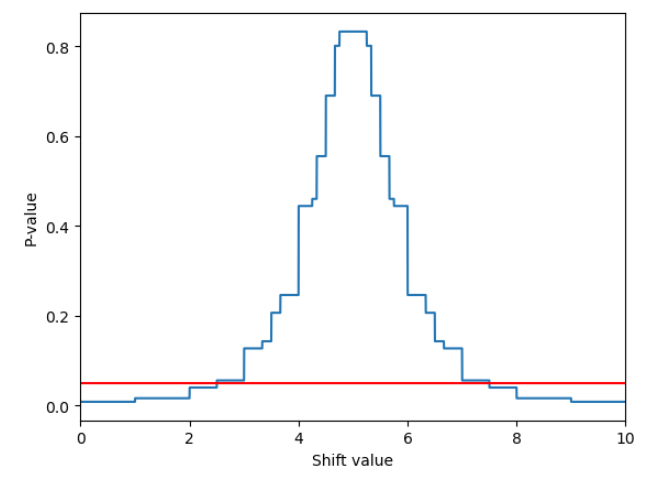
Figure 1: Exemplar (full-group) permutation $P$-value for the two-sided, two-sample shift problem as a function of the hypothesized shift, using the difference in sample means as the test statistic. The two samples are $\{5,6,7,8,9\}$ and $\{0,1,2,3,4\}$. The $P$-value is piecewise constant, discontinuous, and quasiconcave. Many algorithms for inverting permutation tests to form confidence sets incorrectly assume that the $P$-value is continuous in the parameter $\eta$ and equal to $\alpha$ at exactly two values of $\eta$. In the general case, the two-sided $P$-value for the two-sample shift problem using the difference in sample means (i) is equal to $\alpha$ on two intervals, (ii) is equal to $\alpha$ on one interval and jumps through $\alpha$ at a discontinuity, or (iii) jumps through $\alpha$ at two discontinuities. The red horizontal line intersects the plot of the $P$-value as a function of the shift at values where the $P$-value equals 0.05. In this example, the $P$-value jumps through 0.05 at two discontinuities.

The quasiconcavity makes it straightforward to find the endpoints of a conservative confidence interval for the shift to any desired precision, for instance, by using bisection in a conservative way; see Section 5.

The values of some test statistics for different permutations of the data and for different hypothesized values of the parameter have a simple relationship that makes even more computational savings possible, obviating the need to compute the test statistic from scratch for each Monte Carlo iteration for each hypothesized value of the parameter.

This paper is organized as follows. Section 2 gives an overview of randomized tests, $P$-values, and the duality between tests and confidence sets, highlighting the fact that a confidence set derived by inverting hypothesis tests is conservative or exact if and only if the test of the true null is conservative or exact. Section 3 reviews some Monte Carlo tests that are exact or conservative despite relying on simulation. The general approach to computing confidence sets developed below can be used with any of them. Section 4 describes how to construct confidence intervals for real-valued parameters when the $P$-value is quasiconcave in the hypothesized value of the parameter, using the bisection method with a slight modification. Section 5 improves that result for two problems with additional structure: finding a confidence interval for the shift in one-sample and two-sample problems with real-valued data. Section 6 compares the run time and confidence bounds for the new approach with those of some other methods. Section 7 discusses extensions and provides additional context.

2 Randomized tests

Suppose we have a family of probability distributions $\{\mathbb{P}_{\eta}:\eta\in\Theta\}$ on the measurable space $\mathcal{X}$, indexed by the abstract parameter $\eta\in\Theta$. We will observe data $X\sim{\mathbb{P}}_{\theta}$ for some $\theta\in\Theta$. We want to make tests and confidence sets for $\theta$ using $X$, possibly relying in addition on an independent, auxiliary random variable $U$.

We treat the auxiliary randomness $U$ abstractly: it is not necessarily a uniformly distributed real-valued random variable, as is common in the Neyman-Pearson framework. In the examples below, $U$ comprises randomness arising from Monte Carlo sampling.

For each $\eta\in\Theta$, let $\phi_{\eta}(x,u):(\mathcal{X},\mathcal{U})\rightarrow\{0,1\}$ be the rejection function for a level $\alpha$ test of the hypothesis $\theta=\eta$: reject the hypothesis $\theta=\eta$ for data $X=x$ and auxiliary randomness $U=u$ iff $\phi_{\eta}(x,u)=1$. The test defined by $\phi_{\eta}$ has significance level $\alpha$ for the hypothesis $\theta=\eta$ iff

$$\mathbb{E}_{\eta}\phi_{\eta}(X,U)\leq\alpha,$$ (1)

where the expectation is with respect to the joint distribution of $X$ and $U$ computed on the assumption that $\theta=\eta$. The test is exact if equality holds in inequality 1; otherwise, it is conservative.

The duality between tests and confidence sets establishes that the set of all $\eta\in\Theta$ for which the hypothesis $X\sim\mathbb{P}_{\eta}$ would not be rejected at level $\alpha$ is a $1-\alpha$ confidence set for $\theta$:

Theorem 1 (see, e.g., Lehmann et al. [23], § 3.5).

For each $\phi\in\Theta$, let $\phi_{\eta}(x,u):(\mathcal{X},\mathcal{U})\rightarrow\{0,1\}$ be the rejection function for a test of the hypothesis $\theta=\eta$ at significance level $\alpha$. Define $S(X,U):=\{\eta\in\Theta:\phi_{\eta}(X,U)=0\}$. Then if the observed data $X=x$ and the auxiliary randomness $U=u$, $S(x,u)$ is a (possibly randomized) $1-\alpha$ confidence set for $\theta$.

Proof.

$${\mathbb{P}}_{\theta}\{S(X,U)\ni\theta\}={\mathbb{P}}_{\theta}\{\phi_{\theta}(X,U)<1\}\geq 1-\alpha,$$ (2)

where the probability is with respect to the joint distribution of $X\sim{\mathbb{P}}_{\theta}$ and $U$. ∎

Remark 1

The proof of Theorem 1 shows that the coverage probability of the confidence set rides entirely on the fact that the (single) test of the true null $\eta=\theta$ has level $\alpha$. The tests involving other values of $\eta\in\Theta$ play no role whatsoever. In particular, the tests of different nulls do not need to be valid simultaneously; dependence among them does not matter; and a single $U$ can be used for every test. Hence, if the Monte Carlo test of the true null $\theta=\eta$ is exact or conservative, a single set of simulations (i.e., a single realization of $U$) can be used to test every $\eta\in\Theta$.

Section 3.2 gives examples of exact and conservative Monte Carlo tests. Many of the tests we consider are derived from $P$-values, random variables with distributions that are stochastically dominated by the uniform distribution on $[0,1]$ when the null hypothesis is true: $P_{\eta}=P_{\eta}(X,U)$ is a $P$-value for the hypothesis $\theta=\eta$ iff

$${\mathbb{P}}_{\eta}\{P_{\eta}(X,U)\leq p\}\leq p,\;\;\;\forall p\in[0,1],$$ (3)

where the probability is with respect to the joint distribution $X$ and $U$. If equality holds in inequality 3 for every $p$, the $P$-value is exact; otherwise, it is conservative. If $P_{\eta}$ is a $P$-value, then (in the previous notation)

$$\phi_{\eta}(x,u):=\mathbf{1}_{P_{\eta}(x,u)\leq\alpha}$$

defines a test with significance level $\alpha$.

In turn, many of the $P$-values we consider arise from a test statistic $T:\mathcal{X}\rightarrow\Re$. Monte Carlo simulation can be used to calibrate $T$ to produce conservative or exact $P$-values, as discussed in the next section.

3 Exact and Conservative Monte Carlo Tests

We list exact or conservative versions of the three types of Monte Carlo tests listed above: simulation tests, random permutation tests, and randomization tests. All will depend on a test statistic $T:\mathcal{X}\rightarrow\Re$, and we consider larger values of $T$ to be stronger evidence against the null, i.e., the $P$-value decreases monotonically with $T$. Most of the development does not require additional assumptions about $T$, but in section 5 we show that when $T$ has special structure, additional savings are possible.

All three types of test use Monte Carlo to simulate new data sets and use the test statistic applied to each of those sets to find a $P$-value in various ways. In simulation tests, those sets are simulated directly from the null (possibly using importance sampling). In permutation tests, those sets are generated by applying randomly selected elements of a group to the original data. In randomization tests, those sets are generated by randomly re-allocating the data using the randomization design that was used to collect the original data.

We use $Y_{j}$ to denote the $j$th simulated data set and $n$ to denote the number of simulated data sets. The tests thus involve $X$, $T$, and $\{Y_{j}\}_{j=1}^{n}$.

3.1 Simulation tests

Consider the null hypothesis that $X\sim\mathbb{P}$, where $\mathbb{P}$ is a known distribution. Let $\{Y_{j}\}_{j=1}^{n}$ be IID $\mathbb{P}$. Then the following is a valid $P$-value [2, 4, 5, 11]:

$$P:=\frac{1+\sum_{j}1\{T(Y_{j})\geq T(X)\}}{1+n}.$$ (4)

The proof relies only on the fact that, if the null hypothesis is true, all rank orders of $\{T(X),T(Y_{1}),\ldots,T(Y_{n})\}$ are equally likely. This result can be extended to sampling $\{Y_{j}\}$ from a known “proposal distribution” $\mathbb{Q}$ instead of sampling from the null distribution $\mathbb{P}$. Suppose that $\mathbb{P}$ and $\mathbb{Q}$ are absolutely continuous with respect to a dominating measure $\mathbb{F}$ and that $d\mathbb{P}/d\mathbb{F}(x)=0$ whenever $d\mathbb{Q}/d\mathbb{F}(x)=0$ (i.e., any set with strictly positive probability under $\mathbb{P}$ has strictly positive probability under $\mathbb{Q}$). Let $\{Y_{j}\}_{j=1}^{n}$ be an IID sample from $\mathbb{Q}$. Define the importance weight

$$w(x):=\frac{d\mathbb{P}/d\mathbb{F}}{d\mathbb{Q}/d\mathbb{F}}(x),$$

with the convention $0/0:=0$. Then the following are valid $P$-values [15]:

$$P:=\frac{w(X)+\sum_{j=1}^{n}w(Y_{j})1\{T(Y_{j})\geq T(X)\}}{1+n}$$ (5)

$$P:=\frac{w(X)+\sum_{j=1}^{n}w(Y_{j})1\{T(Y_{j})\geq T(X)\}}{w(X)+\sum_{j=1}^{n}w(Y_{j})}.$$ (6)

In the special case $\mathbb{Q}=\mathbb{P}$, $w\equiv 1$, and both of these reduce to equation 4.

3.2 Random permutation tests

Consider the null hypothesis that the probability distribution $\mathbb{P}$ of the data $X\in\mathcal{X}$ is invariant under some group $\mathcal{G}$ of transformations on $\mathcal{X}$, so that $X\sim g(X)$ for all $g\in\mathcal{G}$.

Random permutation tests involve selecting elements of $\mathcal{G}$ at random. The sample can be selected in a number of ways: with or without replacement, with or without weights, from all of $\mathcal{G}$ or from a subgroup of $\mathcal{G}$; or a randomly selected element of $\mathcal{G}$ can be applied to a fixed subset of $\mathcal{G}$. Below are some valid $P$-values for those sampling approaches.

1. $\{\hat{g}_{i}\}_{j=1}^{n}$ is a uniform random sample (with or without replacement) of size $n$ from $\mathcal{G}$ or a subgroup of $\mathcal{G}$. Let $Y_{j}:=\hat{g}_{j}(X)$. Then

   $$P:=\frac{1+\sum_{j=1}^{n}1\{T(Y_{j})\geq T(X)\}}{1+n}$$ (7)

   is a valid $P$-value [9, 7, 30].

2. $\{g_{j}\}_{j=1}^{n}$ is a fixed subset of $n$ elements of $\mathcal{G}$, not necessarily a subgroup; $\hat{g}$ is drawn uniformly at random from $\mathcal{G}$; and $Y_{j}:=g_{j}\hat{g}^{-1}(X)$.

   $$P:=\frac{\sum_{j=1}^{n}1\{T(Y_{j}))\geq T(X)\}}{n}$$ (8)

   is a valid $P$-value [30].

3. $\mathcal{G}$ is a finite group; $\hat{g}$ is selected at random from $\mathcal{G}$ with probability $p(g)$ of selecting $g\in\mathcal{G}$; and $Y_{j}:=g_{j}\hat{g}^{-1}(X)$.

   $$P:=\sum_{j=1}^{|\mathcal{G}|}p(g_{j})\cdot 1\{T(Y_{j})\geq T(X)\}$$ (9)

   is a valid $P$-value [30].

Note that 7 has the same form as equation 4, but 7 in general involves sampling from the conditional distribution given the orbit of the observed data, while equations 4, 5, and 6 involve sampling from the unconditional distribution. The $P$-values in 8 and 9 involve drawing only one random permutation $\hat{g}$, then applying it to other elements of $\cal{G}$ to create $\{Y_{j}\}_{j=1}^{n}$.

3.3 Randomization tests

Unlike (random) permutation tests, which rely on the invariance of the distribution of $X$ under $\mathcal{G}$ if the null is true, randomization tests rely on the fact that generating the data involved randomizing units to treatments (in reality or hypothetically).

Suppose there are $N$ units, each of which is assigned to one of $K$ possible treatments, $t=1,\ldots K$. A treatment assignment $r$ assigns a treatment to each unit: it is a mapping from $\{1,\ldots,N\}$ to $\{1,\ldots,K\}^{N}$. The assignment might use simple random sampling, Bernoulli sampling, blocking, or stratification; the assignment probabilities might depend on covariates. Let $\mathcal{R}$ be the set of treatment assignments the original randomization design might have produced, and let $p(r)$ be the probability that the original randomization made the assignment $r$, for $r\in\mathcal{R}$. Let $r_{0}$ denote the actual treatment assignment.

The test statistic $T$ depends on the data $X^{\prime}$ and the (observed) treatment assignment $r_{0}$; we combine the two into a single random variable $X=(X^{\prime},r_{0})$ and write $T(X)$. Suppose we draw a weighted random sample of $n$ treatment assignments $R_{j}\in\mathcal{R}$, $j=1,\ldots,n$, with or without replacement, with probability $p(r)$ of selecting $r\in\mathcal{R}$ in the first draw (adjusting the selection probabilities appropriately in subsequent draws if the sample is without replacement). Let $Y_{j}:=(X^{\prime},R_{j})$, $j=0,\ldots,n$. Then

$$P:=\frac{\sum_{j=0}^{n}p(R_{j})\cdot 1\{T(Y_{j})\geq T(X)\}}{\sum_{j=0}^{n}p(R_{j})}$$ (10)

is a valid $P$-value. Note that 10 has the same form as 6, and when all $r\in\mathcal{R}$ are equally likely, 10 has the same form as 4 and 7.

Another valid $P$-value has the same form as 9 and involves a weighted sum over all possible assignments, just as 9 involves a weighted sum over all group elements. Let $Y_{j}:=(X^{\prime},r_{j})$, $r_{j}\in\mathcal{R}$. Then

$$P:=\sum_{j=1}^{|\mathcal{R}|}p(r_{j})\cdot 1\{T(Y_{j})\geq T(X)\}$$ (11)

is a valid $P$-value [19, 22, 40, 30].

3.4 Tests about parameters

The tests above do not explicitly involve parameters. They can be extended to a family of tests, one for each possible parameter value $\eta\in\Theta$, in various ways.

For example, suppose there is a bijection $f_{\eta}:\mathcal{X}\rightarrow\mathcal{X}$ such that for any $\mathbb{P}_{0}$-measurable set $A$, $f_{\eta}(A)$ is $\mathbb{P}_{\eta}$-measurable and $\mathbb{P}_{\eta}(f_{\eta}(A))=\mathbb{P}_{0}(A)$, and for any $\mathbb{P}_{\eta}$-measurable set $A$, $f_{\eta}^{-1}(A)$ is $\mathbb{P}_{0}$-measurable and $\mathbb{P}_{\eta}(A)=\mathbb{P}_{0}(f_{\eta}^{-1}(A))$. Then a $P$-value for the hypothesis $\theta=\eta$ can be calculated by using $T(f_{\eta}^{-1}(X))$ and $\{T(f_{\eta}^{-1}(Y_{j}))\}$ in place of of $T(X)$ and $\{T(Y_{j})\}$ in 4, 7, or 8.

One common example is a location family with location parameter $\theta\in\Theta\subset\Re^{m}=\mathcal{X}$. For any $\mathbb{P}_{\mathbf{0}}$-measurable set $A\in\mathcal{X}$, $\mathbb{P}_{\eta}(A):=\mathbb{P}_{\mathbf{0}}(A-\eta)$. In other words, $f_{\eta}(x)=x+\eta$ and $f_{\eta}^{-1}(x)=x-\eta$. A test of the hypothesis $\theta=\mathbf{0}$ can be used to test the hypothesis $\theta=\eta$ by applying the test to the transformed data $X-\eta$ and the transformed values $\{Y_{j}-\eta\}$.

For simulation test $P$-values using importance sampling (definitions 5 and 6) we can test the hypothesis $\theta=\eta$ by using the weights $w_{\eta}(x):=d\mathbb{P}_{\eta}/d\mathbb{Q}$; nothing else needs to be changed. In particular, the same sample can be used.

4 Confidence sets for scalar parameters

Remark 1, above, notes that it suffices to use a single set of Monte Carlo simulations to test the hypothesis $\theta=\eta$ for all $\eta\in\Theta$. As mentioned in section 3.4, how the simulations can be re-used depends on how the test depends on the parameter $\eta$. We use $P(\eta)$ to denote the $P$-value of the hypothesis $\theta=\eta$, $\eta\in\Theta$ for the family of tests under consideration. We now explore a simple case in more detail: confidence intervals for scalar parameters.

4.1 Confidence intervals when the $P$-value is quasiconcave

Suppose that the parameter $\theta$ is a scalar and that $T$ is defined in such a way that $P(\eta)$ is quasiconcave in $\eta$, i.e., if $\eta_{1}$, $\eta_{2}\in\Theta$ with $\eta_{1}\leq\eta_{2}$, then for all $\eta\in[\eta_{1},\eta_{2}]$,

$$P(\eta)\geq\min\{P(\eta_{1}),P(\eta_{2})\}.$$ (12)

(The two-sample test using the difference in sample means as the test statistic has this property.) Then the confidence set—all $\eta\in\Theta$ for which the hypothesis $\theta=\eta$ is not rejected at level $\alpha$—is a connected interval $[\ell,u]$. The lower endpoint $\ell$ is the largest $\eta$ such that $P(\zeta)\leq\alpha$ for all $\eta\in(-\infty,\eta]$; the upper endpoint $u$ is the smallest $\eta$ such that $P(\zeta)\leq\alpha$ for all $\eta\in[\eta,\infty)$.

Quasiconcavity makes it straightforward to find $\ell$ and $u$ (or to approximate them conservatively to any desired precision) using the bisection method with a slight modification to account for the fact that $P(\eta)$ is not continuous in general (see, e.g., 1). Algorithm 1 returns a value in $[u,u+e]$ for any specified tolerance $e>0$. An analogous algorithm returns a value in $[\ell-e,\ell]$.

Algorithm 1 Bisection algorithm for the upper endpoint $u$ of a confidence interval when the $P$-value is quasiconcave in the parameter

1:Set $\alpha\in(0,1)$ and $e>0$, the acceptable amount by which the returned upper endpoint exceeds the true upper endpoint. Let $P(\eta)$ be a valid $P$-value for the hypothesis $\theta=\eta$.

2:Find an interval $[L,U]$ that contains $u$: $P(L)\geq\alpha\geq P(U)$.

3:While $|U-L|>e$:

4:a: Set $m\leftarrow(L+U)/2$.

5:b: If $P(m)>\alpha$, set $L\leftarrow m$, otherwise set $U\leftarrow m$.

6:Return $U$.

5 Additional efficiency in the one-sample and two-sample shift problems

For the most common test statistics, the computational cost of finding each $P$-value can be reduced further in the one-sample and two-sample problems by saving the treatment assignments (or in some cases, just a one-number summary of each assignment: see equation 14) and the value of the test statistic for each treatment assignment [25, 29]. This section explains how.

The one-sample problem.

The one-sample problem is to find a confidence interval for the center of symmetry of a distribution that is symmetric about an unknown point $\theta$ from an IID sample $X=\{X_{j}\}_{j=1}^{n}$ from that distribution.

For any two $N$-vectors $\mathbf{x}$, $\mathbf{y}$, define the componentwise product $\mathbf{x}\odot\mathbf{y}:=(x_{1}y_{1},\ldots,x_{N}y_{N})$. If $\theta=\eta$, the distribution of $X_{j}-\eta$ is symmetric around 0, i.e., conditional on $|X_{j}-\eta|$, $X_{j}-\eta$ is equally likely to be $\pm(X_{j}-\eta)$.

A common test statistic for the hypothesis $\theta=\eta$ is the sum of the signed differences from $\eta$:

$$T_{\eta}(\bm{x}):=\sum_{j=1}^{N}(x_{j}-\eta).$$ (13)

Random permutation tests for the one-sample problem involve the distribution of the test statistic when the signs of $\{X_{j}-\eta\}$ are randomized independently. Let $\bm{\sigma}\in\{-1,1\}^{N}$ be IID uniform random signs. Then we can test the hypothesis $\theta=\eta$ by comparing the value of $T_{\eta}(\mathbf{X})$ to the values of $T_{\eta}(\bm{\sigma}\odot\mathbf{X})$ for $n$ randomly generated vectors $\bm{\sigma}$. As noted above in section 4, we can re-use the values of $\bm{\sigma}$ when testing $\theta=\eta$ for different values of $\eta$. But we can save even more computation by relating the value of $T_{\eta}(\bm{\sigma}\odot\mathbf{X})$ to the value of $T_{0}(\bm{\sigma}\odot\mathbf{X})$:

$$T_{\eta}(\bm{\sigma}\odot\mathbf{x}) = \sum_{j=1}^{N}\sigma_{j}(x_{j}-\eta)$$ (14)

$$= \sum_{j=1}^{N}\sigma_{j}x_{j}-\sum_{j}\sigma_{j}\eta$$

$$= T_{0}(\bm{\sigma}\odot\mathbf{X})-\eta\sum_{j}\sigma_{j}.$$

Thus, for each configuration of signs $\bm{\sigma}$, we need only keep track of $T_{0}(\bm{\sigma}\odot\mathbf{X})$ and $\sum_{j}\sigma_{j}$ to determine the value of the test statistic for any other hypothesized value of $\eta$.

The two-sample problem.

The two-sample problem involves a set of $n$ units and two “conditions,” treatment and control. Each unit will be assigned either to treatment or to control. If unit $j$ is assigned to control, its response will be $y_{j}(0)$; if it is assigned to treatment, its response will be $y_{j}(1)$. The two-sample problem assumes that there is some $\theta\in\Re$ such that for all $j$, $y_{j}(1)-y_{j}(0)=\theta$. Units are assigned to treatment or control by randomly allocating $m$ units into treatment and the remaining $n-m$ to control by simple random sampling, with $n$ and $m$ fixed in advance. We seek a confidence interval for $\theta$ from the resulting data. Let $\{X_{1},\ldots,X_{m}\}$ denote the responses of the units assigned to treatment and let $\{X_{m+1},\ldots,X_{n}\}$ denote the responses of the units assigned to control.

A common test statistic is the difference between the mean response of the treatment group and the mean response of the control group, $\frac{1}{m}\sum_{j=1}^{m}X_{j}-\frac{1}{m-n}\sum_{j=m+1}^{n}X_{j}$, or its Studentized version [39]. Randomization tests for the two-sample problem involve the distribution of the test statistic when units are randomly allocated into treatment and control using the same randomization design the original experiment used.

If an allocation assigns $n_{tc}$ of the units originally assigned to treatment to the control group (and vice-versa), then the difference between the test statistic when the shift is zero and the test statistic when the shift is $\eta$ is

$$T_{\eta}(\mathbf{x})-T_{0}(\mathbf{x})=\eta\cdot n_{tc}\left(\frac{1}{n}+\frac{1}{m}\right).$$ (15)

This result is implicit in Pitman [29]; it is straightforward to show. Suppose that for a particular allocation, the responses of the treatment group are $\{x_{i}\}_{i=1}^{n}$ and the responses of the control group are $\{y_{i}\}_{i=1}^{m}$. Then, the difference in means can be written

$$\frac{m\sum x_{i}-n\sum y_{i}}{nm}.$$

For each of the $n_{tc}$ units that switch from treatment to control (and vice-versa) the change in the test statistic is $\frac{m\eta-n(-\eta)}{nm}=\eta(\frac{1}{n}+\frac{1}{m})$. If $n_{tc}$ units change their treatment assignment, the total change in the test statistic is given by equation 15.

Thus, as we saw for the one-sample problem, for each allocation we only need to keep track of the test statistic for $\eta=0$ and the number of units that moved from treatment to control to find the value of the test statistic for that allocation for any other value of $\eta$. Section 6 gives numerical examples.

6 Comparison to previous methods

6.1 Examples of extant methods

Many proposed methods for finding confidence bounds using random permutation or randomization tests implicitly or explicitly work with the full-group (or all-possible-allocations) $P$-value $P(\eta)$ and assume it is continuous and crosses $\alpha$ at two points. But in practice, $P(\eta)$—whether defined using the full group (or full set of allocations) or only a subset of them—is typically a step function (see Figure 1).

Instead of using random permutations, Tritchler [38] calculates the full-group $P$-value by taking advantage of the fact that the probability distribution of a sum is the convolution of the probability distributions, which becomes a product in the Fourier domain. The proof that their algorithm works relies on Theorem 1 of Hartigan [16] regarding “typical values,” which in turn assumes that the data have a continuous distribution. Despite the fact that the method computes the distribution of the sum efficiently, it evaluates that distribution at such a large number of points that in practice it is limited to small problems.

In contrast, Garthwaite [12] uses random permutations, applying the Robbins-Monro stochastic optimization algorithm [31] to find the endpoints of the confidence interval. It is not guaranteed to give conservative or exact confidence intervals. The Robbins-Monro algorithm is a stochastic iterative method for approximating a root of a function of the expectation of a random variable by using realizations of the random variable. It assumes that the function is strictly monotone at the root, which is assumed to be unique.

The algorithm is sensitive to the starting point. Garthwaite and Jones [13] propose averaging the results of the last $n^{*}$ iterations of the Garthwaite [12] algorithm to increase efficiency. The step size in the Garthwaite [12] algorithm is a function of the significance level $\alpha$, a constant $c>0$, and the step number $i$: either $-c\alpha/i$ or $c(1-\alpha)/i$. This choice of step size can cause the algorithm to get stuck far from any root. O’Gorman [26] show that the Garthwaite [12] and Garthwaite and Jones [13] algorithms can produce very different confidence bounds, even with the same starting point; they recommend averaging eight different runs with the same starting point. This increases the computational burden but still provides no guarantee that the algorithm finds the correct confidence bounds.

Bardelli [1] use random permutations. They propose using the bisection algorithm to find the endpoints, but each step involves a new set of Monte Carlo simulations. That both increases the computational burden and makes the bisection potentially unstable, because sampling variability can make the simulation $P$-value non-monotonic in the shift. Indeed, re-evaluating the $P$-value at the same value of $\eta$ with a different Monte Carlo sample will generally give a different result. Moreover, as mentioned previously, the usual bisection method relies on continuity, but the $P$-value is not typically continuous in the shift.

6.2 Numerical comparisons

The new method has time complexity $O(n)$ for the one-sample and two-sample problems. Our implementation uses the cryptorandom Python library, which provides a cryptographic quality PRNG based on the SHA256 cryptographic hash function (see section 7). That PRNG requires substantially more computation than the Mersenne Twister (MT), the default in R, Python, MATLAB, and many other languages and packages. For instance, generating $10^{7}$ pseudo-random integers between 1 and $10^{7}$ using cryptorandom takes 16s on our machine, in contrast to 0.17s for the numpy implementation of MT: a factor of about 100. We nonetheless advocate using the higher-quality PRNG, especially for large problems, for the reasons given in [36].

Comparison to Tritchler [38]

We first compare results for the one-sample problem in Tritchler [38] using Darwin’s data on the differences in heights of 15 matched pairs of cross-fertilized and self-fertilized plants. Table 1 reports full-group confidence intervals generated by enumeration, the confidence intervals reported by Tritchler [38], and the confidence intervals generated by our method using $n=10^{4}$ and $e=10^{-8}$. It took 0.5s of CPU time to generate the confidence intervals on an Apple MacBook Pro running macOS 12.3, with an M1 Max chip and 64GB of unified memory. Open-source python code that generated the intervals in column 4 is available at https://github.com/akglazer/monte-carlo-ci.

confidence level	full-group	Tritchler	new method
90%	[3.75, 38.14]	[3.75, 38.14]	[3.857, 38.250]
95%	[-.167, 41.0]	[-.167, 41.0]	[-0.167, 41.0]
99%	[-9.5, 47.0]	[-9.5, 47.0]	[-8.80, 47.20]

Table 1: One-sample confidence intervals at 90%, 95%, and 99% computed using the full group of $2^{15}$ reflections, the intervals reported by Tritchler [38], and the intervals computed using our proposed method with $n=10^{4}$ and $e=10^{-8}$, for data on 15 matched pairs of plants:
$49,-67,8,6,16,23,28,41,14,29,56,24,75,60,-48,49.$

We do not have access to source code for the Tritchler [38] method nor to a CDC 6600, so we are unable to compare run times of our method to those of Tritchler [38]. However, Tritchler [38] notes that execution time increases from 3.2s to 11.2s if ten more observations are included, about a 250% increase. On the other hand, the execution time for the new method (with $n=10^{4}$) increased from 0.5s to 0.67s, about a 31% increase.

Next we consider the two-sample problem example in Tritchler [38], which uses data reported in Snedecor and Cochran [34] on the effect of sleep on the basal metabolism (measured in calories per square meter per hour) of 26 college women. The data are listed in table 2.

7+ hours of sleep	35.3, 35.9, 37.2, 33.0, 31.9, 33.7, 36.0, 35.0, 33.3, 33.6, 37.9, 35.6, 29.0, 33.7, 35.7
0–6 hours of sleep	32.5, 34.0, 34.4, 31.8, 35.0, 34.6, 33.5, 33.6, 31.5, 33.8, 34.6

Table 2: Basal metabolism (measured in calories per square meter per hour) and hours of sleep of 26 college women (source: Tritchler [38]).

Full-group confidence intervals generated by enumeration, the confidence intervals reported by Tritchler [38], and the conservative confidence intervals generated by our method using $n=10^{4}$ and $e=10^{-8}$ are given in table 3. Tritchler [38] note that their FORTRAN implementation took 2.6s of CPU time on a CDC 6600, increasing to 14.5s (a 458% increase) when the number of observations was doubled. The new method took 0.60s to execute on our machine, increasing to 0.82s (a 37% increase) if the number of observations is doubled.

confidence level	full-group	Tritchler	new method
90%	[-2.114, 0.386]	[-2.114, 0.386]	[-2.117, 0.380]
95%	[-2.34, 0.650]	[-2.34, 0.650]	[-2.333, 0.643]
99%	[-2.814, 1.180]	[-2.814, 1.180]	[-2.850, 1.167]

Table 3: Two-sample confidence intervals at 90%, 95%, and 99% computed using the full group of $\binom{26}{11}$ reflections, the intervals reported by Tritchler [38], and the intervals computed using our proposed method with $n=10^{4}$ and $e=10^{-8}$, for the basal metabolism data in table 2. The fourth column is based on a single seed value.

For larger sample sizes, Tritchler [38]’s method quickly becomes infeasible, but the new method still runs relatively quickly. For example, for groups of $1,000$ units each, our new method takes approximately 22s to execute using the cryptorandom PRNG and approximately 5s for the numpy.random.random MT implementation, both using $10^{4}$ samples and $e=10^{-8}$.

Comparison to Garthwaite [12]

Garthwaite [12] gives an example involving the effect of malarial infection on the stamina of the lizard Sceloporis occidentali. The data are listed in table 4.

infected lizards ($X$)	16.4, 29.4, 37.1, 23.0, 24.1, 24.5, 16.4, 29.1, 36.7, 28.7, 30.2, 21.8, 37.1, 20.3, 28.3
uninfected lizards ($Y$)	22.2, 34.8, 42.1, 32.9, 26.4, 30.6, 32.9, 37.5, 18.4, 27.5, 45.5, 34.0, 45.5, 24.5, 28.7

Table 4: Distance in meters run in two minutes by infected and uninfected lizards (source: Samuels et al. [33], as reported by Garthwaite [12]).

Garthwaite [12] reports $[-0.30,10.69]$ as the nominal 95% confidence interval based on 6000 steps of his algorithm; as mentioned above, that interval is approximate, not exact or conservative. Our implementation of the Garthwaite algorithm produced the approximate confidence interval $[-0.29,11.0]$ in 0.72s, using 6000 steps and the initial values of 0 and 10 for the lower and upper endpoints. For $n=6000$ using the $P$-value defined in 7, the new algorithm yields the conservative confidence interval $(-0.20,10.875)$ in 0.38s.

7 Discussion

This paper presents an efficient method for constructing exact or conservative Monte Carlo confidence intervals from exact or conservative Monte Carlo tests. The method uses a single set of Monte Carlo samples. That solves two problems: it reduces the computational burden of testing all possible null values of the parameter, and it ensures that the problem of finding where the $P$-value crosses $\alpha$ is well posed, in the sense that it involves finding where a fixed function crosses a threshold rather than involving different realizations for each function evaluation. For problems with real-valued parameters, if the $P$-value is quasiconcave in the parameter, a minor modification of the bisection algorithm quickly finds conservative confidence bounds to any desired degree of precision. Additional computational savings are possible for common test statistics in the one-sample and two-sample problem by exploiting the relationship between values of the test statistics for different values of the parameter.

How many Monte Carlo samples?

The tests and confidence intervals we consider are exact or conservative regardless of how many or how few Monte Carlo samples $n$ are used, so computation time can be reduced by using fewer samples. However, the highest attainable non-trivial confidence level is $n/(n+1)$. Increasing the number of samples also reduces the variability of results from seed to seed, and tends to approximate more precisely the bounds that would be obtained by examining all possible samples, permutations, or allocations.

The PRNG matters

Many common PRNGs—including the Mersenne Twister, the default PRNG in R, Python, MATLAB, SAS, and STATA (version 14 and later)—have state spaces that are too small for large problems [36]. Depending on the problem size, they cannot even generate all samples or all permutations, much less generate them with equal probability. Linear congruential generators (LCGs) are especially limited; even a 128-bit LCG can generate only about 0.03% of the possible samples of size 25 from a set of 500 items. The Mersenne Twister cannot in principle generate all permutations of set of 2084 items, and can generate less than $2\times 10^{-6}$ of the possible samples of size 1,000 from $10^{8}$ items. The choice of algorithms for generating samples or permutations from the PRNG also matters: a common algorithm for generating a sample—assign a pseudorandom number to each item, sort on that number, and take the first $k$ items to be the sample—requires a much higher-quality PRNG than algorithms that generate the sample more directly [36]. For large problems, a cryptographic quality PRNG may be needed. A Python implementation of a PRNG that uses the SHA256 cryptographic hash function is available at https://github.com/statlab/cryptorandom.

Where is the computational cost?

In our examples for the one-sample and two-sample problems, the bulk of the CPU time is in generating the (single) Monte Carlo sample, especially when using the (expensive) cryptorandom SHA256 PRNG. The bisection stage of the algorithm is extremely fast; increasing $e$ from $10^{-8}$ to $10^{-6}$ has a trivial effect on runtimes.

Confidence sets for percentiles of an effect in the two-sample problem

In the two-sample problem, the null hypothesis $\theta=\eta$ is that the shift for every unit is $\eta$. Caughey et al. [6] show that this hypothesis and the corresponding confidence set can be interpreted as a hypothesis test and confidence set for the maximum and minimum of the shift even when the shift varies from unit to unit, and how to use similar calculations to find confidence bounds for percentiles of the shift.

Nuisance parameters

Sometimes $\theta$ is multidimensional but we are only interested in a functional $f$ of $\theta$, e.g., its weighted mean, a component, a contrast, or some other linear or nonlinear functional. There are three general strategies to obtain conservative confidence bounds for $f(\theta)$ when there are nuisance parameters:

• Define the $P$-value to be the maximum $P$-value over all values of the nuisance parameters that correspond to the hypothesized value of the parameter of interest, in effect decomposing a composite null into a union of simple nulls and rejecting the composite iff every simple null is rejected [8, 24, 27].

• Define the $P$-value for the composite hypothesis to be the maximum $P$-value over a confidence set for the nuisance parameters [3].

• Construct a confidence set for the entire parameter $\theta$, then define the endpoints of the confidence interval for $f(\theta)$ as the supremum and infimum of $f$ over the confidence set. This is sometimes called strict bounds [10, 37].

The general strategy of re-using the Monte Carlo sample to test different hypothesized values of the parameter can be used with any of these.

7.1 Software

We are aware of only a few packages or repositories with code to compute confidence intervals for the one- or two-sample problem. The CIPerm R package constructs intervals for the two-sample problem based on the algorithm in Nguyen [25]. While this implementation uses a single set of permutations, it uses a brute-force search for the endpoints, which Nguyen [25] note is time-consuming. Another R package, Perm.CI, only works for binary outcomes and uses a similarly inefficient brute force method. Other implementations, such as that in Caughey et al. [6] use the function uniroot, an implementation of Brent’s method, which incorrectly assumes the $P$-value is continuous in $\eta$.

Open-source Python software implementing the new methods presented in this paper is available at https://github.com/akglazer/monte-carlo-ci.

Acknowledgments.

This work was supported in part by NSF Grants DGE 2243822 and SaTC 2228884. We are grateful to Benjamin Recht for helpful conversations.

References

- Bardelli [2016] C. Bardelli. Nonparametric Confidence Intervals Based on Permutation Tests. PhD thesis, Politecnico Di Milano, 2016.
- Barnard [1963] G. Barnard. Discussion of the spectral analysis of point processes. Journal of the Royal Statistical Society Series B, 25, 1963.
- Berger and Boos [1994] R. L. Berger and D. D. Boos. P values maximized over a confidence set for the nuisance parameter. Journal of the American Statistical Association, 89(427):1012–1016, 1994.
- Birnbaum [1974] Z. W. Birnbaum. Reliability and Biometry, chapter Computers and unconventional test-statistics, pages 441–458. Philadelphia: SIAM, 1974.
- Bølviken and Skovlund [1996] E. Bølviken and E. Skovlund. Confidence intervals from monte carlo tests. Journal of the American Statistical Association, 91(435):1071–1078, 1996.
- Caughey et al. [2017] D. Caughey, A. Dafoe, and L. Miratrix. Beyond the sharp null: Randomization inference, bounded null hypotheses, and confidence intervals for maximum effects. arXiv preprint arXiv:1709.07339, 2017.
- Davison and Hinkley [1997] A. C. Davison and D. V. Hinkley. Bootstrap methods and their application. Cambridge university press, 1997.
- Dufour [2006] J.-M. Dufour. Monte carlo tests with nuisance parameters: A general approach to finite-sample inference and nonstandard asymptotics. Journal of econometrics, 133(2):443–477, 2006.
- Dwass [1957] M. Dwass. Modified randomization tests for nonparametric hypotheses. The Annals of Mathematical Statistics, 28:181–187, 1957.
- Evans and Stark [2002] S. N. Evans and P. B. Stark. Inverse problems as statistics. Inverse problems, 18(4):R55–R97, 2002.
- Foutz [1980] R. V. Foutz. A method for constructing exact tests from test statistics that have unknown null distributions. Journal of Statistical Computation and Simulation, 10(3-4):187–193, 1980.
- Garthwaite [1996] P. H. Garthwaite. Confidence intervals from randomization tests. Biometrics, 52:1387–1393, 1996.
- Garthwaite and Jones [2009] P. H. Garthwaite and M. C. Jones. A stochastic approximation method and its application to confidence intervals. Journal of Computational and Graphical Statistics, 18:184–200, 2009.
- Good [2006] P. I. Good. Resampling methods. Springer, 2006.
- Harrison [2012] M. T. Harrison. Conservative hypothesis tests and confidence intervals using importance sampling. Biometrika, 99(1):57–69, 2012.
- Hartigan [1969] J. A. Hartigan. Using subsample values as typical values. Journal of the American Statistical Association, 64:1303–1317, 1969.
- Hemerik [2024] J. Hemerik. On the term “randomization test”. The American Statistician, pages 1–8, 2024.
- Hemerik and Goeman [2018] J. Hemerik and J. Goeman. Exact testing with random permutations. TEST, 27:811–825, 2018. doi: 10.1007/s11749-017-0571-1.
- Hemerik and Goeman [2021] J. Hemerik and J. J. Goeman. Another look at the lady tasting tea and differences between permutation tests and randomisation tests. International Statistical Review, 89(2):367–381, 2021.
- Higgins [2004] J. J. Higgins. An introduction to modern nonparametric statistics. Brooks/Cole Pacific Grove, CA, 2004.
- Imbens and Rubin [2015] G. W. Imbens and D. B. Rubin. Causal inference in statistics, social, and biomedical sciences. Cambridge university press, 2015.
- Kempthorne and Doerfler [1969] O. Kempthorne and T. Doerfler. The behaviour of some significance tests under experimental randomization. Biometrika, 56(2):231–248, 1969.
- Lehmann et al. [2005] E. L. Lehmann, J. P. Romano, and G. Casella. Testing statistical hypotheses, volume 3. New York: springer, 2005.
- Neyman and Pearson [1933] J. Neyman and E. S. Pearson. On the problem of the most efficient tests of statistical hypotheses. Philosophical Transactions of the Royal Society of London. Series A, Containing Papers of a Mathematical or Physical Character, 231:289–337, 1933.
- Nguyen [2009] M. Nguyen. Nonparametric Inference Using Randomization and Permutation Reference Distribution and Their MonteCarlo Approximation. PhD thesis, Portland State University, 2009.
- O’Gorman [2014] T. W. O’Gorman. Regaining confidence in confidence intervals for the mean treatment effect. Statistics in medicine, 33:3859–3868, 2014.
- Ottoboni et al. [2018] K. Ottoboni, P. B. Stark, M. Lindeman, and N. McBurnett. Risk-limiting audits by stratified union-intersection tests of elections (suite). In International Joint Conference on Electronic Voting, pages 174–188. Springer, 2018.
- Pagano and Tritchler [1983] M. Pagano and D. Tritchler. On obtaining permutation distributions in polynomial time. Journal of the American Statistical Association, 78(382):435–440, 1983.
- Pitman [1937] E. J. Pitman. Significance tests which may be applied to samples from any populations. Supplement to the Journal of the Royal Statistical Society, 4(1):119–130, 1937.
- Ramdas et al. [2023] A. Ramdas, R. F. Barber, E. J. Candès, and R. J. Tibshirani. Permutation tests using arbitrary permutation distributions. Sankhya A, pages 1–22, 2023.
- Robbins and Monro [1951] H. Robbins and S. Monro. A stochastic approximation method. The Annals of Mathematical Statistics, pages 400–407, 1951.
- Salmaso and Pesarin [2010] L. Salmaso and F. Pesarin. Permutation tests for complex data: theory, applications and software. John Wiley & Sons, 2010.
- Samuels et al. [2003] M. L. Samuels, J. A. Witmer, and A. A. Schaffner. Statistics for the life sciences, volume 4. Prentice Hall Upper Saddle River, NJ, 2003.
- Snedecor and Cochran [1967] G. Snedecor and W. Cochran. Statistical Methods, volume 6. Ames, Iowa: Iowa State University Press, 1967.
- Splawa-Neyman et al. [1990] J. Splawa-Neyman, D. M. Dabrowska, and T. P. Speed. On the application of probability theory to agricultural experiments. essay on principles. section 9. Statistical Science, pages 465–472, 1990.
- Stark and Ottoboni [2018] P. Stark and K. Ottoboni. Random sampling: Practice makes imperfect. arXiv preprint arXiv:1810.10985, 2018.
- Stark [1992] P. B. Stark. Inference in infinite-dimensional inverse problems: discretization and duality. Journal of Geophysical Research: Solid Earth, 97(B10):14055–14082, 1992.
- Tritchler [1984] D. Tritchler. On inverting permutation tests. Journal of the American Statistical Association, 79:200–207, 1984.
- Wu and Ding [2021] J. Wu and P. Ding. Randomization tests for weak null hypotheses in randomized experiments. Journal of the American Statistical Association, 116(536):1898–1913, 2021.
- Zhang and Zhao [2023] Y. Zhang and Q. Zhao. What is a randomization test? Journal of the American Statistical Association, 118(544):2928–2942, 2023.