Conv-Basis: A New Paradigm for Efficient Attention Inference and Gradient Computation in Transformers

Large Language Models (LLMs) have profoundly changed the world. Their self-attention mechanism is the key to the success of transformers in LLMs. However, the quadratic computational cost $O(n^{2})$ to the length $n$ input sequence is the notorious obstacle for further improvement and scalability in the longer context. In this work, we leverage the convolution-like structure of attention matrices to develop an efficient approximation method for attention computation using convolution matrices. We propose a $\mathsf{conv}$ basis system, “similar” to the rank basis, and show that any lower triangular (attention) matrix can always be decomposed as a sum of $k$ structured convolution matrices in this basis system. We then design an algorithm to quickly decompose the attention matrix into $k$ convolution matrices. Thanks to Fast Fourier Transforms (FFT), the attention inference can be computed in $O(knd\log n)$ time, where $d$ is the hidden dimension. In practice, we have $d\ll n$, i.e., $d=3,072$ and $n=1,000,000$ for Gemma. Thus, when $kd=n^{o(1)}$, our algorithm achieve almost linear time, i.e., $n^{1+o(1)}$. Furthermore, the attention training forward and backward gradient can be computed in $n^{1+o(1)}$ as well. Our approach can avoid explicitly computing the $n\times n$ attention matrix, which may largely alleviate the quadratic computational complexity. Furthermore, our algorithm works on any input matrices. This work provides a new paradigm for accelerating attention computation in transformers to enable their application to longer contexts.

1 Introduction

Numerous notable large language models (LLMs) in natural language processing (NLP) have emerged in these two years, such as BERT [23], OPT [118], PaLM [20], Mistral [54], Gemini [102], Gemma [105], Claude3 [5], GPT-3 [10], GPT-4 [1], Llama [104], Llama2 [106], Llama3 [4] and so on. These models have profoundly changed the world and have been widely used in human activities, such as education [58], law [95], finance [69], bio-informatics [107], coding [49], and even creative writing [1] such as top AI conference reviews [61]. The key component of the generative LLMs success is the decoder-only transformer architecture introduced by [108]. The transformer uses the self-attention mechanism, allowing the model to capture long-range dependencies in the input sequence. Self-attention computes a weighted sum of the input tokens, where the weights are determined by the similarity between each pair of tokens. This enables the model to attend to relevant information from different parts of the sequence when generating the output. However, the computational complexity of the self-attention in transformers grows quadratically $O(n^{2})$ with the input length $n$, limiting their applicability to long context, e.g., 128k, 200k, 1000k input tokens for GPT4 [1], Claude3 [5], Gemma [105] respectively.

The bottleneck complexity $O(n^{2})$ comes from computing the similarity between each pair of tokens, which will introduce an $n\times n$ size matrix. More specifically, let $d$ be the hidden dimension and let $Q,K\in\mathbb{R}^{n\times d}$ be the query and key matrices of input. Then, we can see $QK^{\top}\in\mathbb{R}^{n\times n}$. Although $QK^{\top}$ is at most rank-$d$, $\mathsf{softmax}(QK^{\top})\in\mathbb{R}^{n\times n}$ may be full rank in softmax attention.

To overcome the complexity obstacle of $\mathsf{softmax}(QK^{\top})$, many works study more efficient attention computation methods that can scale almost linearly with the sequence length while maintaining the model’s performance. [6] show that if all entry of $QK^{\top}$ is bounded and $d=O(\log n)$, $\mathsf{softmax}(QK^{\top})$ will be “close” to a low-rank matrix. Then, they present an algorithm that can approximate attention computation in almost linear time. Similarly, by uniform softmax column norms assumption and sparse assumption, [47] solve attention computation in almost linear time, where they identify large entries in the attention matrix and only focus on them.

On the other hand, many works [74, 101, 73, 80] find that the attention pattern has $\mathsf{conv}$-like (or “diagonalized”) structure (see Figure 1 (b)), mathematically, $A_{i,j}\approx A_{i^{\prime},j^{\prime}}$ when $i-j=i^{\prime}-j^{\prime}$, where we can see $i-j$ as the position distance between two tokens. It is relevant to the bag-of-words or $n$-gram concept, i.e., $n$ adjacent symbols or words in NLP. Furthermore, the $\mathsf{conv}$-like structure can be connected to convolution recurrent models [9] and structured state space models (SSMs) as Mamba [35]. More specifically, we can use multiple convolution matrices to approximate an attention matrix, whose intuition is similar to the low-rank approximation in the sense of computation acceleration. Note that the matrix product of a convolution matrix and a vector can be computed by Fast Fourier Transform (FFT) with time complexity $O(n\log(n))$, while the naive way takes $O(n^{2})$ time (see details in Figure 1 (a)). Therefore, it is natural to ask:

Can we use the convolution matrix to accelerate the attention computation?

The answer is positive. In this paper, we use multiple convolution matrices to approximately solve the attention computation efficiently. Informally speaking, we have the following results which can apply to any $Q,K\in\mathbb{R}^{n\times d}$.

Theorem 1.1 (Main result (informal Theorem 4.4)).

Let $\epsilon>0$, $k\in[n]$ and $Q,K\in\mathbb{R}^{n\times d}$. If $QK^{\top}$ is $\epsilon$-close ($\ell_{\infty}$ norm) to a matrix with $k$-$\mathsf{conv}$ basis (Definition 4.1), then we can solve the Exact Attention Computation task (Definition 3.3) in $O(knd\log(n))$ time via FFT with error up to $O(\epsilon)$.

When $kd=n^{o(1)}$, we get almost linear time $n^{1+o(1)}$ by our method. Similarly to the low-rank approximation, in our work, we build up a $\mathsf{conv}$ basis system, “similar” to the rank basis, and show that any lower triangular matrix $H\in\mathbb{R}^{n\times n}$ can always be decomposed into $k$-$\mathsf{conv}$ basis for some $k\in[n]$ (Lemma 3.12 and Theorem 4.3). Then, our Algorithm 2 can quickly decompose $QK^{\top}$ into $k$ convolution matrix when $QK^{\top}$ satisfying some non-degenerate properties (see properties in Definition 4.1). Finally, via FFT, we only need time complexity $O(knd\log(n))$ to solve the task (Algorithm 1 and Theorem 4.4), while the naive methods require $O(n^{2}d)$.

Thus, our algorithm can achieve attention inference in $O(knd\log(n))$, without needing any parameter updates e.g., re-train or finetune. Our theorems can also applied to accelerate attention training [7]. In detail, our methods take $O(dkn\log n+nd^{2})$ time for forward computation and $O(d^{2}kn\log n)$ time for backward gradient computation (Theorem 5.6). Furthermore, applying our technique to low-rank approximation of attention matrices [6], we can extend their results to more general settings (Theorem 6.5). In detail, [6] only works on attention approximation without an attention mask, while ours can be applied to different kinds of attention masks including the most popular causal attention mask (Definition 3.2). It shows the broad applicability of our analysis. We summarize our contributions below.

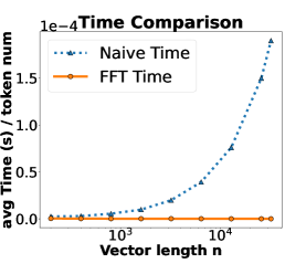
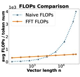
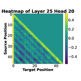
Figure 1: (a) In the left two figures, we compare the complexity of $\mathsf{conv}(a)\cdot w$ between the Naive way and FFT way, where random vector $a,w\in\mathbb{R}^{n}$ and $\mathsf{conv}(a)\in\mathbb{R}^{n\times n}$ (Definition 3.5). The $x$-axis is the input token number $n$. The $y$-axis is the average CPU time/Float Operations (FLOPs) over $n$, in the first/second figure. The number reported is an average of 100 runs with the Numpy implementation. It is clear to see the Naive way takes $O(n^{2})$ while the FFT way takes $O(n\log n)$. (b) In the right figure, we plot one $QK^{\top}\in\mathbb{R}^{n\times n}$ in Llama3 [4], where input is from the SST-2 [111] with $n=47$ tokens. It is clear to see the $\mathsf{conv}$-like structure in the attention matrix.

Detailed comparison with previous works.

Our results are beyond or comparable to the two brilliant previous works in the following sense. (1) To guarantee a small approximation error, for the attention matrix, [6] needs bounded entries assumption and $d=O(\log n)$ assumption, while [47] needs uniform softmax column norms assumption and sparse assumption. However, without all these assumptions, our algorithm can still guarantee a small approximation error (Corollary 4.5), i.e., our algorithm can apply to any $Q,K$ including unbounded matrices, dense matrices, and any hidden dimension $d$. (2) To guarantee a truly subquadratic running time, [6] needs to assume $d=O(\log n)$ to get $n^{1+o(1)}$ time complexity. However, for our algorithm, as long as $d=n^{o(1)}$ and $k=n^{o(1)}$, we achieve running time $n^{1+o(1)}$. This has much less restriction on $d$. Moreover, our time complexity covers from $n^{1+o(1)}$ to $n^{2-\Omega(1)}$ with different $d$, while [6] can only handle $d=O(\log n)$. (3) To guarantee a truly subquadratic running time, [47] needs to assume $dm=n^{2-\Omega(1)}$, as they get $O(dn^{1+o(1)}+dm)$ time complexity where $m$ is the number of large entries in attention matrices. Our work gets $O(knd\log(n))$ time complexity and we need $kd=n^{1-\Omega(1)}$ to get truly subquadratic running time. For the situation $m=n^{1+o(1)},d=n^{o(1)}$ and $k=n^{o(1)}$, both our algorithm and [47] run in $n^{1+o(1)}$ time. For the situation $m=n^{1+\Omega(1)}$, $d=n^{o(1)}$ and $k=n^{o(1)}$, running time in [47] will be truly super-linear $n^{1+\Omega(1)}$ while our algorithm remains almost $n^{1+o(1)}$ linear time.

Our contributions.

• We build up a $\mathsf{conv}$ basis system, and show that any lower triangular matrix $H\in\mathbb{R}^{n\times n}$ can always be decomposed into $k$-$\mathsf{conv}$ basis for some $k\in[n]$ (Lemma 3.12 and Theorem 4.3).

• Our algorithm can quickly decompose any lower triangular matrix into its $k$ convolution basis (Algorithm 2), so, via FFT, we can solve Exact Attention Computation task in $O(knd\log(n))$ (Algorithm 1 and Corollary 4.5). When $kd=n^{o(1)}$, our method takes almost linear time $n^{1+o(1)}$. Our results are beyond or comparable to previous works (see comparison above).

• During attention inference, our algorithm takes $O(knd\log(n))$, without needing any parameter updates e.g., re-train or fine-tune (Theorem 4.4). It may enable further improvement and scalability of LLMs in the longer context.

• During attention training, our methods take $O(dkn\log n+nd^{2})$ time for forward computation and $O(d^{2}kn\log n)$ time for backward gradient computation (Theorem 5.6). It may save time, resources, and energy for nowadays LLMs training.

• Our broad applicable technique can be applied to the low-rank approximation of attention matrices and extend existing results to more general settings (Theorem 6.5).

Roadmap.

In Section 2, we introduce the related work. In Section 3, we present the background for this paper. In Section 4, we present our algorithms and mathematical analysis for the convolution approximation for attention computation. In Section 5, we present the $\mathsf{conv}$ approximation during training forward and backward gradient. In Section 6, we explain how to apply our technique to the low-rank approximation. In Section 7, we discuss two case studies: Longlora and RoPE.

2 Related Work

Attention matrix $\mathsf{conv}$-like structure.

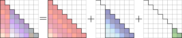
Figure 2: A matrix with $3$-$\mathsf{conv}$ basis. We present an example of the matrix defined in Definition 3.11 when $k=3$. The matrix with $3$-$\mathsf{conv}$ basis is on the left-hand side of the equation in this figure. The red entries in this matrix come from the first matrix on the right-hand side. The purple entries in this matrix are the sum of the red entries from the first matrix on the right-hand side and the blue entries from the second matrix on the right-hand side. The dark green entries are equal to the sum of red, green, and blue entries from the matrices on the right-hand side.

Very recent works study the $\mathsf{conv}$-like attention matrix. [31, 74] find that in-context learning is driven by the formation of “induction heads”–attention heads that copy patterns from earlier in the input sequence. This is reflected in the attention matrix becoming more diagonal, with tokens attending primarily to preceding tokens that match the current token. In [101] Figure 6, they show a similar $\mathsf{conv}$-like attention pattern for other important attention circuits. Figure 3 of [80] shows that in a minimal classification task, the abrupt emergence of in-context learning coincides with the formation of an induction head, characterized by a diagonal attention pattern. [73] proves that for a simplified task, gradient descent causes a transformer to encode the causal graph structure of the task in the attention matrix. This results in tokens attending primarily to their causal parents reflected in a sparse diagonal structure (Figure 2).

Fast attention computation and long context LLM.

The development of efficient attention computation has been an active area of research in recent years. The standard self-attention mechanism, introduced in the transformer architecture [108], has a quadratic complexity with respect to the sequence length, which limits its applicability to long sequences. To address this limitation, various approaches have been proposed to improve the efficiency of attention computation. One line of research focuses on patterns of sparse attention that reduce the number of computations [14, 11, 117, 83, 47]. Another approach is to use low-rank approximations or random features for the attention matrix [81, 62, 110, 18, 119, 6, 2], which reduces the computational complexity to linear in the sequence length. In addition, using linear attention as a proxy of softmax attention is a rich line of work [103, 59, 85, 116, 84, 2, 96, 113, 115, 29]. These developments in efficient attention computation have enabled transformer-based models to process longer sequences and have opened up new possibilities for their application in various domains [21, 82, 76, 30, 72, 114, 3, 8, 51].

Convolution in language model and FFT.

There are many subquadratic-time architectures are proposed to address Transformers’ computational inefficiency on long sequences, gated convolution recurrent models [9, 33, 75, 79], and structured state space models (SSMs) [36, 35]. They can use global or local convolution [57] operations to replace attention while keeping a comparable performance. The convolution operation can be computed by fast Fourier transform (FFT) efficiently [78, 16]. Moreover, the development of efficient convolution algorithms like Winograd [60] and FFT-based convolutions [70] has further optimized the computation, reducing the memory footprint and improving the overall speed. There are many other works studying Fourier transform [77, 71, 17, 88, 67, 19, 91, 39, 92, 22, 99, 53].

3 Preliminary

In Section 3.1, we introduce the basic definitions and mathematical properties. In Section 3.2, we give the formal definition of the sub-convolution matrix and present it basic properties.

Notations.

We use $\circ$ to denote element-wise multiplication. We denote $[n]=\{1,2,\dots,n\}$ and $[0]$ as an empty set. We denote ${\bf 0}_{n}$ and ${\bf 1}_{n}$ as the $n$-dimensional vector whose entries are all $0$ and $1$ respectively. Similarly, ${\bf 0}_{n\times n}$ and ${\bf 1}_{n\times n}$ represent the $n\times n$ matrices whose entries are all 0 and 1 respectively. We denote $\exp(\cdot)$ as the element-wise exponential function. For any arbitrary positive integer $n$, for all $x\in\mathbb{R}^{n}$, we use $x_{i}\in\mathbb{R}$ to denote the $i$-th entry of $x$. We denote $[x_{a},x_{a+1},\dots,x_{b}]^{\top}\in\mathbb{R}^{b-a+1}$ as $x_{a:b}$, where $1\leq a\leq b\leq n$, similarly for matrix. Let $\operatorname{diag}:\mathbb{R}^{n}\to\mathbb{R}^{n\times n}$ be defined as $\operatorname{diag}(x)_{i,i}=x_{i}$ and $\operatorname{diag}(x)_{i,j}=0$, for all $i\neq j$.

For a matrix $A\in\mathbb{R}^{m\times n}$, we define its $\ell_{1}$ norm as $\|A\|_{1}=\sum_{i=1}^{m}\sum_{j=1}^{n}|A_{ij}|$, $\ell_{\infty}$ norm as $\|A\|_{\infty}=\max_{i,j}|A_{ij}|$ (usually we also call it matrix max norm), and Frobenius norm as $\|A\|_{F}:=\sqrt{\sum_{i,j}A_{i,j}^{2}}$, where $A_{ij}$ is an entry of $A$ at the $i$-th row and $j$-th column.

3.1 Basic Definitions and Facts about Attention and $\mathsf{conv}$

Now, we present basic definitions. We start by introducing the input and weight matrix.

Definition 3.1 (Input and weight matrix).

We define the input sequence as $X\in\mathbb{R}^{n\times d}$ and the key, query, and value weight matrix as $W_{K},W_{Q},W_{V}\in\mathbb{R}^{d\times d}$. Then, we define the key, query, and value matrix as $Q:=XW_{Q}$, $K:=XW_{K}$, $V:=XW_{V}$.

It is straightforward to see $QK^{\top}=XW_{Q}W_{K}^{\top}X^{\top}$. In generative LLMs, there is a causal attention mask $M$ to guarantee the later tokens cannot see the previous tokens during generation. It is defined as follows:

Definition 3.2 (Causal attention mask).

We define the causal attention mask as $M\in\{0,1\}^{n\times n}$, where $M_{i,j}=1$ if $i\geq j$ and $M_{i,j}=0$ otherwise. We define $M_{j}$ be the $j$-th column of $M$.

Now, we are ready to introduce the mathematical definition of the exact attention computation with a mask.

Definition 3.3 (Exact attention computation).

Let $Q,K,V\in\mathbb{R}^{n\times d}$ be the query, key, and value matrices respectively defined in Definition 3.1. Let $M\in\{0,1\}^{n\times n}$ be the attention mask defined in Definition 3.2. The goal of the Exact Attention Computation is to find the matrix $\mathrm{Att}(M,Q,K,V)\in\mathbb{R}^{n\times d}$, which is defined as

$$\mathrm{Att}(M,Q,K,V):=D^{-1}AV$$

where $A\in\mathbb{R}^{n\times n}$ is a lower triangular matrix and $D\in\mathbb{R}^{n\times n}$ is a diagonal matrix, i.e.,

$$A:=M\circ\exp(QK^{\top}),\quad\text{and}\quad D:=\mathrm{diag}(A{\bf 1}_{n}).$$

Remark 3.4.

In Definition 3.3, we divide the $\mathsf{softmax}$ operation into an element-wise $\exp$ operation and a diagonal normalization matrix $D$ to obtain a clear formulation.

Efficiently computing the attention needs to exploit structured matrices that enable fast multiplication algorithms. Here, we define the convolution matrix, which is a structured matrix where each row vector is rotated one element to the right relative to the preceding row vector, which is defined as follows:

Definition 3.5 (Convolution matrix).

Let $a\in\mathbb{R}^{n}$ denote a length-$n$ vector. We define $\mathsf{conv}:\mathbb{R}^{n}\rightarrow\mathbb{R}^{n\times n}$ as,

$$\mathsf{conv}(a):=\begin{bmatrix}a_{1}&0&0&\cdots&0\\ a_{2}&a_{1}&0&\cdots&0\\ a_{3}&a_{2}&a_{1}&\cdots&0\\ \vdots&\vdots&\vdots&\ddots&\vdots\\ a_{n}&a_{n-1}&a_{n-2}&\cdots&a_{1}\end{bmatrix}.$$

By the following fact, we know that the rank of a convolution matrix can be an arbitrary number. Thus, our $\mathsf{conv}$-basis is totally different from the rank basis.

Claim 3.6.

We have $\mathsf{conv}(e_{j})\in\mathbb{R}^{n\times n}$ is a $j$-rank matrix, where the $j$-th entry of $e_{j}\in\mathbb{R}^{n}$ is $1$ and all other entries are $0$.

Proof.

The proof is trivial by Definition 3.5. ∎

Efficient computation of the convolution operation is crucial for many applications. The convolution theorem states that the circular convolution of two vectors can be computed efficiently using the Fast Fourier Transform (FFT). This leads to the following claim (see proof in Appendix A.1):

Claim 3.7.

Let $\mathsf{conv}$ be defined in Definition 3.5. For any $a,x\in\mathbb{R}^{n}$, $\mathsf{conv}(a)x$ can be computed in $O(n\log n)$ via FFT.

One property of convolution matrices is that they are additive with respect to the input vectors. In other words, the convolution of the sum of two vectors is equal to the sum of the convolutions of the individual vectors. This is stated formally in the following claim:

Claim 3.8.

$\mathsf{conv}$ is additive, i.e., for any $a,b,x\in\mathbb{R}^{n}$ we have

$$\mathsf{conv}(a)x+\mathsf{conv}(b)x=\mathsf{conv}(a+b)x.$$

Proof.

This is trivial by Definition 3.5 and matrix product operation is additive. ∎

3.2 Sub-convolution Matrix: Definitions and Properties

If we would like to use $\mathsf{conv}$ as a basis system, we need to introduce some new concepts. Recall that, in general, the sum of two rank-1 matrices is a rank-2 two matrix. Due to $\mathsf{conv}$ being additive, the sum of two convolution matrices is another convolution matrix, which does not hold the above property. Thus, we need to introduce sub-convolution matrices to be the basis.

Definition 3.9 (Sub-convolution matrix).

Let $m\in[n]$. For any $a\in\mathbb{R}^{n}$. We define the sub-convolution matrix $\mathsf{conv}(a,m)$ as

$$\mathsf{conv}(a,m)=\begin{bmatrix}{\bf 0}_{(n-m)\times(n-m)}&{\bf 0}_{(n-m)\times m}\\ {\bf 0}_{m\times(n-m)}&\mathsf{conv}(a_{1:m})\end{bmatrix}.$$

Given two vectors $a,x\in\mathbb{R}^{n}$, let $a*_{m}x\in\mathbb{R}^{n}$ denote the sub-convolution operator between $a$ and $x$, i.e., $\mathsf{conv}(a,m)x=a*_{m}x$.

Similarly, sub-convolution can be computed in $O(n\log n)$ time via FFT.

Claim 3.10.

Let $m\in[n]$. For any $a,x\in\mathbb{R}^{n}$, $\mathsf{conv}(a,m)x$, (defined in Definition 3.9) can be computed in $O(n\log n)$ via FFT.

Proof.

This is trivial by considering the calculation between the truncated matrix of $\mathsf{conv}(a,m)$ and the truncated vector of $x$ with Claim 3.7. ∎

Here, we present the definition of the matrix with $k$-$\mathsf{conv}$ basis which is non-reducible.

Definition 3.11 (Matrix with $k$-$\mathsf{conv}$ basis).

Let $k\in[n]$. We say a lower triangular matrix $H\neq{\bf 0}_{n\times n}\in\mathbb{R}^{n\times n}$ has $k$-$\mathsf{conv}$ basis if

• There exists $b_{1},\dots,b_{k}\in\mathbb{R}^{n}$ and $k$ integers $m_{1},m_{2},\dots,m_{k}$ satisfying $n\geq m_{1}>m_{2}>\dots>m_{k}\geq 1$ such that $H=\sum_{i\in[k]}\mathsf{conv}(b_{i},m_{i}),$ (defined in Definition 3.9).

• For any $b_{1},\dots,b_{k-1}\in\mathbb{R}^{n}$ and $k-1$ integers $m_{1},m_{2},\dots,m_{k-1}$ satisfying $n\geq m_{1}>m_{2}>\dots>m_{k-1}\geq 1$ we have $H\neq\sum_{i\in[k-1]}\mathsf{conv}(b_{i},m_{i}).$

The following lemma establishes that any non-zero lower triangular matrix can be represented as a matrix with a $k$-$\mathsf{conv}$ basis for some unique $k$ between $1$ and $n$. The proof is Appendix D.1.

Lemma 3.12.

For any lower triangular matrix $H\neq{\bf 0}_{n\times n}\in\mathbb{R}^{n\times n}$, there exists a unique $k\in[n]$ such that $H$ is a matrix with $k$-$\mathsf{conv}$ basis.

4 $\mathsf{conv}$ Approximation during Inference

In Section 4.1, we introduce the basic definitions to support our algorithmic analysis in this section. In Section 4.2, we present the binary search and recover $k$-$\mathsf{conv}$ algorithms and present their theoretical guarantees. In Section 4.3, we provide the formal version of our main result.

4.1 Key Concepts

Recall that any non-zero lower triangular matrix can be represented as a matrix with a $k$-$\mathsf{conv}$ basis for some unique $k$ between $1$ and $n$ (Lemma 3.12). However, exactly getting $k$ is hard and the definition is too strict for the algorithm design. Thus, for more flexibility, we introduce a more general definition of non-degenerate $k$-$\mathsf{conv}$ basis as below, which is a proxy notion to relax the conditions required in algorithm design.

Definition 4.1 (Non-degenerate $k$-$\mathsf{conv}$ basis).

Let $T\in[n]$, $\delta\geq 0$, and $k\in[n+1-T]$. Let $b_{1},\dots,b_{k}\in\mathbb{R}^{n}$ and $k$ integers $m_{1},m_{2},\dots,m_{k}$ satisfying $n\geq m_{1}>m_{2}>\dots>m_{k}\geq T$. Let $H=\sum_{i\in[k]}\mathsf{conv}(b_{i},m_{i})$. If for each basis $i\in[k]$, for all $j\in[i]$, we have $\|\sum_{l=j}^{i}(b_{l})_{1:T}\|_{1}\geq\delta$, then we define $H\in\mathbb{R}^{n\times n}$ to be a matrix with $(T,\delta)$-non-degenerate $k$-$\mathsf{conv}$ basis.

Here $(T,\delta)$-non-degenerate $k$-$\mathsf{conv}$ basis means that each $\mathsf{conv}$ basis cannot be “covered” by the other basis easily.

Definition 4.2.

We define $G$ as a $\epsilon$-close $(T,\delta)$-non-degenerate $k$-$\mathsf{conv}$ basis matrix when $G=H+R$, where $H$ is a $(T,\delta)$-non-degenerate $k$-$\mathsf{conv}$ basis matrix defined in Definition 4.1 and the noise matrix $R\in\mathbb{R}^{n\times n}$ satisfies $\|R\|_{\infty}\leq\epsilon\leq\frac{\delta}{5T}$.

The following theorem establishes that any non-zero lower triangular matrix can be represented as an $\epsilon$-close $(T,\delta)$-non-degenerate $k$-$\mathsf{conv}$ basis matrix. There may be many different choices of $(k,T,\delta,\epsilon)$, which provide flexibility for our Algorithm 1.

Theorem 4.3.

For any lower triangular matrix $G\neq{\bf 0}_{n\times n}\in\mathbb{R}^{n\times n}$, there exists $k,T\in[n]$ and $\delta,\epsilon\geq 0$ such that $G$ is a $\epsilon$-close $(T,\delta)$-non-degenerate $k$-$\mathsf{conv}$ basis matrix.

Proof.

By Lemma 3.12, we have $G$ is a matrix with $k$-$\mathsf{conv}$ basis for some $k\in[n]$. We finish the proof by setting $T=1$ and $\delta=\epsilon=0$. ∎

4.2 Algorithms and Their Properties

Now, we present our main Algorithm 1. We also present Algorithm 2 and Algorithm 3 being used.

Algorithm 1 Main $k$-$\mathsf{conv}$ forward

1:procedure $\mathsf{conv}$Forward($Q,K,V\in\mathbb{R}^{n\times d},k,T\in[n],\delta,\epsilon\in\mathbb{R}_{\geq 0}$)

2:     $\widetilde{b}_{1},\dots,\widetilde{b}_{k},m_{1},\dots,m_{k}\leftarrow$ Recover($Q,K,k,T,\delta,\epsilon$) $\triangleright$ Algorithm 2

3:     $\widetilde{D}\leftarrow\operatorname{diag}(\sum_{r\in[k]}\mathsf{conv}(\widetilde{b}_{r},m_{r}){\bf 1}_{n})$ by FFT in Claim 3.10

4:     $\widetilde{Y}\leftarrow\widetilde{D}^{-1}\sum_{r\in[k]}\mathsf{conv}(\widetilde{b}_{r},m_{r})V$ by FFT in Claim 3.10

5:     return $\widetilde{Y}$

6:end procedure

Algorithm 2 Recover $k$-$\mathsf{conv}$

1:procedure Recover($Q,K\in\mathbb{R}^{n\times d},k,T\in[n],\delta,\epsilon\in\mathbb{R}_{\geq 0}$)

2:     $v\leftarrow{\bf 0}_{T},u\leftarrow{\bf 0}_{n},s\leftarrow 0,t\leftarrow n-T+1$

3:     for $i=1\to k$ do

4:         $s\leftarrow s+1$

5:         $s\leftarrow$ Search($Q,K,k,T,\delta,\epsilon,v,s,t$) $\triangleright$ Algorithm 3

6:         $m_{i}\leftarrow n-s+1$

7:         $\widetilde{H}_{s}\leftarrow M_{s}\circ(Q(K^{\top})_{s})$

8:         $(b^{\prime}_{i})_{1:m_{i}}\leftarrow\widetilde{H}_{s,s:s+m_{i}-1}-u_{1:m_{i}}$, $(b^{\prime}_{i})_{m_{i}+1:n}\leftarrow{\bf 0}_{n-m_{i}}$

9:         $v\leftarrow v+(b^{\prime}_{i})_{1:T}$

10:         $u\leftarrow u+b^{\prime}_{i}$

11:     end for

12:     Get $\widetilde{b}_{1},\dots,\widetilde{b}_{k}$ by Lemma A.13 from $b^{\prime}_{1},\dots,b^{\prime}_{k}$ and $m_{1},\dots,m_{k}$

13:     return $\widetilde{b}_{1},\dots,\widetilde{b}_{k},m_{1},\dots,m_{k}$

14:end procedure

Algorithm 3 Binary search

1:procedure Search($Q,K\in\mathbb{R}^{n\times d},k,T\in[n],\delta,\epsilon\in\mathbb{R}_{\geq 0},v\in\mathbb{R}^{T},s,t\in[n]$)

2:     if $s\geq t$ then

3:         return $s$

4:     end if

5:     $j\leftarrow\lfloor(s+t)/2\rfloor$

6:     $\widetilde{H}_{j}\leftarrow{M_{j}}\circ{(Q(K^{\top})_{j})}$ $\triangleright$ $j\in[n],M$ is attention mask defined in Definition 3.2

7:     $\alpha\leftarrow\|(\widetilde{H}_{j})_{j:j+T-1}-v\|_{1}$

8:     if $\alpha\geq\delta-2T\epsilon$ then

9:         return Search($Q,K,k,T,\delta,\epsilon,v,s,j$)

10:     else

11:         return Search($Q,K,k,T,\delta,\epsilon,v,j+1,t$)

12:     end if

13:end procedure

4.3 Main Theoretical Result

In this section, we present our main result.

Theorem 4.4 (Main $\mathsf{conv}$ results for inference).

Let $Q,K,V\in\mathbb{R}^{n\times d}$. Recall $A=M\circ\exp(QK^{\top})\in\mathbb{R}^{n\times n}$, $D=\operatorname{diag}(A{\bf 1}_{n})\in\mathbb{R}^{n\times n}$ defined in Definition 3.3. We denote $Y:=D^{-1}AV\in\mathbb{R}^{n\times d}$. Let $M\circ(QK^{\top})$ be a $\epsilon$-close $(T,\delta)$-non-degenerate $k$-$\mathsf{conv}$ basis matrix as defined in Definition 4.2, where $\delta,\epsilon\geq 0$ and $k,T\in[n]$. By Algorithm 1, we can get $\widetilde{Y}$ such that

$$\|Y-\widetilde{Y}\|_{\infty}\leq 2(\exp(2\epsilon)-1)\|V\|_{\infty},$$

whose time complexity is $O(knd\log(n))$ given $M,Q,K,V$.

Proof sketch of Theorem 4.4..

See complete proof in Appendix A.4.

The proof idea is that using binary search to recover all non-degenerate $\mathsf{conv}$ basis (Lemma A.15), which takes $O(nkd\log(n))$ time and has upto $2(\exp(2\epsilon)-1)\|V\|_{\infty}$ error (Lemma A.16). Then, via FFT (Claim 3.10), we finish the proof. ∎

Note that our algorithm can handle any $Q,K\in\mathbb{R}^{d\times d}$. Furthermore, we can exactly recover $Y$ if we do not care about the time complexity. We formally describe the above intuition in the following.

Corollary 4.5 (Exact $\mathsf{conv}$ inference).

Let $Q,K,V\in\mathbb{R}^{n\times d}$. Recall $A=M\circ\exp(QK^{\top})\in\mathbb{R}^{n\times n}$, $D=\operatorname{diag}(A{\bf 1}_{n})\in\mathbb{R}^{n\times n}$ defined in Definition 3.3. We denote $Y:=D^{-1}AV\in\mathbb{R}^{n\times d}$. For any $\epsilon\geq 0$ and any $Q,K,V$, there exists hyper-parameter $k,T\in[n]$ and $\delta\geq 0$ such that Algorithm 1 can output $\widetilde{Y}$ satisfying

$$\|Y-\widetilde{Y}\|_{\infty}\leq 2(\exp(2\epsilon)-1)\|V\|_{\infty},$$

Furthermore, we can exactly get $Y$, i.e., $\epsilon=0$, through Algorithm 1 with time complexity $O(n^{2}d\log(n))$ in the worst case.

Proof.

We set $k=n$, $T=1$, $\delta=0$ and $\epsilon=0$ as the input of Algorithm 1. Then, the proof follows Theorem 4.3 and Theorem 4.4 . ∎

By Theorem 4.4, when $\epsilon=O(1)$, we directly get the attention inference time complexity is $O(knd\log(n))$ with error upto $O(\epsilon)$ as claimed in Section 1. It may enable further improvement and scalability of LLMs in the longer context.

5 $\mathsf{conv}$ Approximation during Training Forward and Backward Gradient

We can apply our algorithm to accelerate attention training including forward and back propagation. We first define the attention training task, which is also used in [7].

Definition 5.1 (Attention optimization).

Given $A_{1},A_{2},A_{3},E\in\mathbb{R}^{n\times d}$ and $Y\in\mathbb{R}^{d\times d}$. we let $M\in\mathbb{R}^{n\times n}$ be a casual attention mask defined in Definition 3.2. We define the attention optimization as

$$\min_{X\in\mathbb{R}^{d\times d}}L(X):=0.5\|D(X)^{-1}M\circ\exp(A_{1}XA_{2}^{\top})A_{3}Y-E\|_{F}^{2}.$$

Here $D(X)\in\mathbb{R}^{n\times n}$ is

$$D(X):=\operatorname{diag}(M\circ\exp(A_{1}XA_{2}^{\top}){\bf 1}_{n}).$$

Remark 5.2.

Our Attention Optimization task in Definition 5.1 covers both the cross-attention and self-attention setting. Let weight matrices $W_{K},W_{Q},W_{V}\in\mathbb{R}^{d\times d}$ be defined in Definition 3.1. For the self-attention setting, we can see $A_{1},A_{2},A_{3}\in\mathbb{R}^{n\times d}$ as $X\in\mathbb{R}^{n\times d}$ in Definition 3.1, see $X\in\mathbb{R}^{d\times d}$ in Definition 5.1 as $W_{Q}W_{K}^{\top}\in\mathbb{R}^{d\times d}$ and see $Y\in\mathbb{R}^{d\times d}$ as $W_{V}\in\mathbb{R}^{d\times d}$. To overcome the quadratic complexity obstacle, we only need to handle the gradient computation of $W_{Q}W_{K}^{\top}$.

Let $x,y\in\mathbb{R}^{d^{2}}$ denote the vectorization of $X,Y\in\mathbb{R}^{d\times d}$. Then, we define some basic notions used.

Definition 5.3.

${\cal T}_{\mathrm{mat}}(n,d,k)$ represents the time of an $n\times d$ matrix times a $d\times k$ matrix.

Definition 5.4 ($\otimes$ Kronecker product).

Given two matrices $A_{1}\in\mathbb{R}^{n_{1}\times d_{1}}$, $A_{2}\in\mathbb{R}^{n_{2}\times d_{2}}$, we define $A:=A_{1}\otimes A_{2}\in\mathbb{R}^{n_{1}n_{2}\times d_{1}d_{2}}$ as follows

$$A_{i_{1}+(i_{2}-1)n_{1},j_{1}+(j_{2}-1)d_{1}}=(A_{1})_{i_{1},j_{1}}\cdot(A_{2})_{i_{2},j_{2}},~{}~{}~{}\forall i_{1}\in[n_{1}],i_{2}\in[n_{2}],j_{1}\in[d_{1}],j_{2}\in[d_{2}].$$

Recall that during inference, we have the $n\times n$ size matrix $QK^{\top}$. Similarly, in gradient calculation, we have an $n\times n$ size matrix, and we denote it as $u(x)$.

Definition 5.5.

Let $M\in\mathbb{R}^{n\times n}$ be a casual attention mask defined in Definition 3.2. Let $A_{1},A_{2}\in\mathbb{R}^{n\times d}$. Suppose that $\operatorname{\mathsf{A}}=A_{1}\otimes A_{2}\in\mathbb{R}^{n^{2}\times d^{2}}$. For all $j_{0}\in[n]$, let $\operatorname{\mathsf{A}}_{j_{0}}\in\mathbb{R}^{n\times d^{2}}$ be the $j_{0}$-th block of $\operatorname{\mathsf{A}}$ and

$$u(x)_{j_{0}}:=\underbrace{M_{j_{0},*}}_{n\times 1}\circ\underbrace{\exp(\operatorname{\mathsf{A}}_{j_{0}}x)}_{n\times 1}.$$

Define $u(x)\in\mathbb{R}^{n\times n}$ as the matrix where the $j_{0}$-th row corresponds to $(u(x)_{j_{0}})^{\top}$.

Then, we are ready to present our main results for attention training.

Theorem 5.6 (Main $\mathsf{conv}$ result for training forward and backward gradient).

If $u(x)$ is a $1/\operatorname{poly}(n)$-close $(T,\delta)$-non-degenerate $k$-$\mathsf{conv}$ basis matrix as defined in Definition 4.2, where $\delta\geq 0$ and $k,T\in[n]$. Then there are algorithms that run to compute training forward in time $O(dkn\log n+{\cal T}_{\mathrm{mat}}(n,d,d))$ and backward gradient in time $O(d^{2}kn\log n)$ of attention loss (Definition 5.1) approximately up to $1/\operatorname{poly}(n)$ error under $\ell_{\infty}$ norm.

Proof sketch of Theorem 5.6..

See complete proof in Appendix B.4.

During backward computation, we can convey the properties of low-rank and convolution at the same time (Lemma B.13 and Lemma B.15). Then, by tensor trick, we can compute the attention gradient based on attention inference (Lemma B.9). We finish the proof by Theorem 4.4. ∎

Remark 5.7.

Note that [7] only needs to convey the low-rank property, while our proof needs to convey the properties of low-rank and convolution simultaneously, which is a more general analysis.

Our Theorem 5.6 shows that our algorithm can accelerate Transformer training as well. It may save time, resources, and energy for nowadays LLMs training.

6 Low Rank Approximation

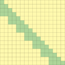
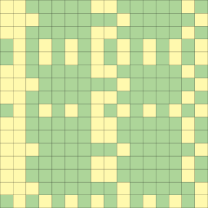
Figure 3: A $16\times 16$ matrix with, left - row change by amortized constant mask (Definition 6.1); middle - continuous row mask (Definition 6.2); right - distinct $3$ rows mask (Definition 6.4). Green means $1$ and yellow means $0$.

We can apply our analysis technique to low-rank approximation setting in [6]. In detail, [6] only works on attention approximation without an attention mask. Equipped with our mask analysis trick, we can generalize their results with different kinds of attention masks including the most popular causal attention mask. We first introduce some practical attention masks.

Definition 6.1.

Let $B_{j}\in\operatorname*{\mathbb{Z}}_{\geq 0}$. We define the row change by amortized constant mask as $W\in\{0,1\}^{n\times n}$, where let $(W^{\top})_{0}={\bf 0}_{n}$ and $\|(W^{\top})_{j}-(W^{\top})_{j-1}\|_{1}\leq B_{j}$ for any $j\in[n]$ and $(W^{\top})_{j}$ is the $j$-th row of $W$.

Definition 6.2.

We define the continuous row mask as $W\in\{0,1\}^{n\times n}$, where for each $i\in[n]$, we are given $s_{i},t_{i}\in[n]$ such that $W_{i,j}=1$ if $s_{i}\leq j\leq t_{i}$ and $W_{i,j}=0$ otherwise.

Definition 6.3.

We define $W\in\{0,1\}^{n\times n}$ as the distinct $r$ columns mask satisfying the following condition. Let $S_{1},\cdots,S_{r}\subseteq[n]$ denote $r$ disjoint subsets and $\cup_{j\in[r]}S_{j}=[n]$. For any two $i,i^{\prime}\in S_{j}$, we have $W_{*,i}=W_{*,i^{\prime}}\in\mathbb{R}^{n}$, where $W_{*,i}\in\mathbb{R}^{n}$ denote the $i$-th column of $W\in\mathbb{R}^{n\times n}$.

Definition 6.4.

We define $W\in\{0,1\}^{n\times n}$ as the distinct $r$ rows mask satisfying the following condition. Let $S_{1},\cdots,S_{r}\subseteq[n]$ denote $r$ disjoint subsets and $\cup_{j\in[r]}S_{j}=[n]$. For any two $i,i^{\prime}\in S_{j}$, we have $W_{i,*}=W_{i^{\prime},*}\in\mathbb{R}^{n}$, where $W_{i,*}\in\mathbb{R}^{n}$ denotes the $i$-th row of $W\in\mathbb{R}^{n\times n}$.

Then, we have the following main results for the low-rank setting. The proof is in Appendix C.2.

Theorem 6.5 (Main low-rank result).

Assume the same condition as Lemma C.2. Let $\epsilon\in(0,0.1)$. Let $Q,K,V\in\mathbb{R}^{n\times d}$. Let $U_{1},U_{2}\in\mathbb{R}^{n\times k}$ be defined in Lemma C.2. Let $W\in\{0,1\}^{n\times n}$ denote a mask matrix. Let $H=\exp(QK^{\top}/d)\in\mathbb{R}^{n\times n}$, $A=W\circ H\in\mathbb{R}^{n\times n}$ and $D=\operatorname{diag}(A{\bf 1}_{n})\in\mathbb{R}^{n\times n}$. We denote $Y:=D^{-1}AV\in\mathbb{R}^{n\times d}$. Let $\widetilde{A}:=W\circ U_{1}U_{2}^{\top}$ and $\widetilde{D}:=\operatorname{diag}(\widetilde{A}{\bf 1}_{n})$. We denote $\widetilde{Y}:=\widetilde{D}^{-1}\widetilde{A}V\in\mathbb{R}^{n\times d}$. Then, we have

$$\|Y-\widetilde{Y}\|_{\infty}\leq 4\epsilon\|V\|_{\infty}.$$

The time complexity to get $\widetilde{Y}$ is

• $O(knd)$ when $W$ is a causal mask defined in Definition 3.2.

• $O(kd\sum_{j=1}^{n}B_{j})$ when $W$ is a row change mask defined in Definition 6.1.

• $O(knd\log(n))$ when $W$ is a continuous row mask defined in Definition 6.2.

• $O(rnd)$ when $W$ is a distinct $r$ columns / rows mask defined in Definition 6.3 / Definition 6.4.

Our Theorem 6.5 has the same error guarantee as [6]. For the normal mask, e.g., casual attention mask (Definition 3.2), Theorem 6.5 shares the same time complexity as theirs.

7 Discussion

In this section, we discuss how to implement our methods in some popular long-context LLMs, e.g., LongLora [21] and the RoPE [82] model family.

LongLora.

Our $\mathsf{conv}$ and low-rank approximation can be applied to LongLora [21], whose mask is shown in the left of Figure 3. They use this kind of sparse mask to extend the context sizes of pre-trained large language models, with limited computation cost, e.g., extending Llama2 70B from 4k context to 32k on a single $8\times$ A100 machine. As the “diagonalized” mask structure, we can directly apply our Algorithm 1 by replacing the causal attention mask (Definition 3.2) with their sparse mask for the $\mathsf{conv}$ approximation with time complexity $O(knd\log(n))$. Similarly, for the low-rank approximation, we directly use the second statement in Theorem 6.5 by considering row change by amortized constant mask defined in Definition 6.1 with time complexity $O(knd)$, where $B_{j}=O(1)$ for any $j\in[n]$.

RoPE.

The Rotary Position Embedding (RoPE) [82] designs a rotation matrix $R^{(m)}\in\mathbb{R}^{d\times d}$, for all $m\in[n]$, which can effectively encode the positional information into embedding $Q,K\in\mathbb{R}^{n\times d}$. In detail, let $q_{i},k_{j}\in\mathbb{R}^{d}$, where $q_{i}^{\top}$ and $k_{j}^{\top}$ be the $i$-th and $j$-th row of $Q,K$ respectively, for any $i,j\in[n]$. By the property of rotation matrix, we have

$$(R^{(i)}q_{i})^{\top}(R^{(j)}k_{j})=q_{i}^{\top}R^{(j-i)}k_{j}$$

We define $Q^{\prime},K^{\prime}\in\mathbb{R}^{n\times d}$, and let $q^{\prime}_{i},k^{\prime}_{j}\in\mathbb{R}^{d}$, where ${q^{\prime}}_{i}^{\top}$ and ${k^{\prime}}_{j}^{\top}$ be the $i$-th and $j$-th row of $Q^{\prime},K^{\prime}$ respectively, for any $i,j\in[n]$. Let $q^{\prime}_{i}=R^{(i)}q_{i}$ and $k^{\prime}_{j}=R^{(j)}k_{j}$. By Equation (34) in [82], we know that we can get $Q^{\prime},K^{\prime}$ in $O(nd)$ time. Thus, we can apply $Q^{\prime},K^{\prime}$ in our Theorem 4.4 and Theorem 6.5 to get the same approximation error guarantee and the same time complexity.

Appendix A Technical Details About $\mathsf{conv}$ Approximation

In Section A.1, we present the background of Toeplitz, circulant, and convolution matrices. In Section A.2, we develop more mathematical tools for studying the $\mathsf{conv}$ approximation. In Section A.3, we give the key lemmas we used. In Section A.4, we use these tools and lemmas to prove our main theorem for the $\mathsf{conv}$ approximation. In Section A.5, we analyze our case study.

A.1 Properties of Toeplitz, Circulant, and Convolution Matrices

Remark A.1.

The integer $i$ may have different ranges. We will specify these ranges in later text, corresponding to different contexts.

The Toeplitz matrix is one such structured matrix that has constant values along its diagonals. We define it as follows:

Definition A.2 (Toeplitz matrix).

Given a length-$(2n-1)$ vector $a\in\mathbb{R}^{2n-1}$ (for convenience, we use $a_{i}\in\mathbb{R}$ to denote the entry of vector where $i\in\{-(n-1),-(n-2),\cdots,0,\cdots,(n-2),(n-1)\}$), we can formulate a function $\mathsf{Toep}:\mathbb{R}^{2n-1}\rightarrow\mathbb{R}^{n\times n}$ as follows

$$\mathsf{Toep}(a)=\begin{bmatrix}a_{0}&a_{-1}&a_{-2}&\cdots&a_{-(n-1)}\\ a_{1}&a_{0}&a_{-1}&\cdots&a_{-(n-2)}\\ a_{2}&a_{1}&a_{0}&\cdots&a_{-(n-3)}\\ \vdots&\vdots&\vdots&\ddots&\vdots\\ a_{n-1}&a_{n-2}&a_{n-3}&\cdots&a_{0}\end{bmatrix}.$$

Furthermore, we define the circulant matrix, which is a structured matrix where each row vector is rotated one element to the right relative to the preceding row vector, which is defined as follows:

Definition A.3 (Circulant matrix).

Let $a\in\mathbb{R}^{n}$ denote a length-$n$ vector. We define $\mathsf{Circ}:\mathbb{R}^{n}\rightarrow\mathbb{R}^{n\times n}$ as,

$$\mathsf{Circ}(a):=\begin{bmatrix}a_{1}&a_{n}&a_{n-1}&\cdots&a_{2}\\ a_{2}&a_{1}&a_{n}&\cdots&a_{3}\\ a_{3}&a_{2}&a_{1}&\cdots&a_{4}\\ \vdots&\vdots&\vdots&\ddots&\vdots\\ a_{n}&a_{n-1}&a_{n-2}&\cdots&a_{1}\end{bmatrix}.$$

Now, we define a binary operation $*$ defined on $\mathbb{R}^{d}$:

Definition A.4.

Let $\mathsf{conv}$ be defined in Definition 3.5. Given two vectors $a$ and $x\in\mathbb{R}^{n}$, let $a*x\in\mathbb{R}^{n}$ denote the convolution operator between $a$ and $x$, i.e., $a*x:=\mathsf{conv}(a)x$.

Finally, we present a basic fact about the Hadamard product.

Fact A.5.

For all $a,b\in\mathbb{R}^{n}$, we have $a\circ b=b\circ a=\mathrm{diag}(a)\cdot b=\mathrm{diag}(b)\cdot a$.

Below, we explore the properties of $\mathsf{conv}$, $\mathsf{Toep}$, $\mathsf{Resi}$, and $\mathsf{Circ}$.

Claim A.6.

Given a length-$(2n-1)$ vector $a^{\prime}\in\mathbb{R}^{2n-1}$ (for convenience, we use $a^{\prime}_{i}\in\mathbb{R}$ to denote the entry of vector where $i\in\{-(n-1),-(n-2),\cdots,0,\cdots,(n-2),(n-1)\}$). Let $a\in\mathbb{R}^{n}$, such that $a=[a^{\prime}_{0},a^{\prime}_{1},\dots,a^{\prime}_{n-1}]^{\top}$. Let $M$ be defined in Definition 3.2, $\mathsf{Toep}$ be defined in Definition A.2, and $\mathsf{conv}$ be defined in Definition 3.5. We have

$$\mathsf{conv}(a)=\mathsf{Toep}(\begin{bmatrix}{\bf 0}_{n-1}\\ a\end{bmatrix})=M\circ\mathsf{Toep}(a^{\prime}).$$

Proof.

The proof directly follows the Definition 3.2, Definition A.2, and Definition 3.5. ∎

Fact A.7 (Folklore).

Let $\mathsf{Toep}$ be defined in Definition A.2, and $\mathsf{Circ}$ be defined in Definition A.3. Given a length-$(2n-1)$ vector $a\in\mathbb{R}^{2n-1}$ (for convenience, we use $a_{i}\in\mathbb{R}$ to denote the entry of vector where $i\in\{-(n-1),-(n-2),\cdots,0,\cdots,(n-2),(n-1)\}$). Let $a^{\prime}\in\mathbb{R}^{2n}$, such that $a^{\prime}=[a_{0},a_{1},\dots,a_{n-1},0,a_{-(n-1)},\dots,a_{-1}]^{\top}$. For any $x\in\mathbb{R}^{n}$, we have

$$\mathsf{Circ}(a^{\prime})\begin{bmatrix}x\\ {\bf 0}_{n}\end{bmatrix}=\begin{bmatrix}\mathsf{Toep}(a)&\mathsf{Resi}(a)\\ \mathsf{Resi}(a)&\mathsf{Toep}(a)\\ \end{bmatrix}\cdot\begin{bmatrix}x\\ {\bf 0}_{n}\end{bmatrix}=\begin{bmatrix}\mathsf{Toep}(a)x\\ \mathsf{Resi}(a)x\\ \end{bmatrix},$$

where the residual matrix is defined as

$$\mathsf{Resi}(a):=\begin{bmatrix}0&a_{n-1}&a_{n-2}&\cdots&a_{2}&a_{1}\\ a_{-(n-1)}&0&a_{n-1}&\cdots&a_{3}&a_{2}\\ a_{-(n-2)}&a_{-(n-1)}&0&\cdots&a_{4}&a_{3}\\ \vdots&\vdots&\vdots&\ddots&\vdots&\vdots\\ a_{-2}&a_{-3}&a_{-4}&\cdots&0&a_{n-1}\\ a_{-1}&a_{-2}&a_{-3}&\cdots&a_{-(n-1)}&0\end{bmatrix}.$$

$\mathsf{Circ}(a)$ can be expressed in the form of $F^{-1}\mathrm{diag}(Fa)F$, which is as follows:

Fact A.8 (Folklore).

Let $a\in\mathbb{R}^{n}$ denote a length-$n$ vector. Let $\mathsf{Circ}$ be defined in Definition A.3. Let $F\in\mathbb{C}^{n\times n}$ denote the discrete Fourier transform matrix. Using the property of discrete Fourier transform, we have

$$\mathsf{Circ}(a)=F^{-1}\mathrm{diag}(Fa)F.$$

Claim A.9 (Restatement of Claim 3.7).

Let $\mathsf{conv}$ be defined in Definition 3.5. For any $a,x\in\mathbb{R}^{n}$, $\mathsf{conv}(a)x$ can be computed in $O(n\log n)$ via FFT.

Proof of Claim 3.7.

For any $a\in\mathbb{R}^{n}$, we denote $a^{\prime}=\begin{bmatrix}{\bf 0}_{n-1}\\ a\\ \end{bmatrix}\in\mathbb{R}^{2n-1}$ and $a^{\prime\prime}=\begin{bmatrix}a\\ {\bf 0}_{n}\\ \end{bmatrix}\in\mathbb{R}^{2n}$. We have

$$\begin{bmatrix}\mathsf{conv}(a)x\\ \mathsf{Resi}(a^{\prime})x\\ \end{bmatrix}= ~{}\begin{bmatrix}\mathsf{Toep}(a^{\prime})x\\ \mathsf{Resi}(a^{\prime})x\\ \end{bmatrix}=\mathsf{Circ}(a^{\prime\prime})\begin{bmatrix}x\\ {\bf 0}_{n}\end{bmatrix}=F^{-1}\mathrm{diag}(Fa^{\prime\prime})F\begin{bmatrix}x\\ {\bf 0}_{n}\end{bmatrix},$$

where the first step follows Claim A.6, i.e., $\mathsf{conv}(a)=\mathsf{Toep}(\begin{bmatrix}{\bf 0}_{n-1}\\ a\end{bmatrix})$, the second step follows Fact A.7 and the last step follows Fact A.8. We finish the proof by $O(n\log n)$ for FFT. ∎

A.2 Mathematical Tools Development for $k$-$\mathsf{conv}$ Basis

Definition A.10.

Let $M\in\mathbb{R}^{n\times n}$ be defined in Definition 3.2 and $Q,K\in\mathbb{R}^{n\times d}$ be defined in Definition 3.1. We define $\widetilde{H}:=M\circ(QK^{\top})\in\mathbb{R}^{n\times n}$.

When a lower triangular matrix $H$ is expressed as the sum of $k$ convolution matrices, it is useful to understand the structure of the entries in $H$. The following claim provides an explicit formula for the entries of $H$ in terms of the basis vectors of the convolution matrices.

Claim A.11.

Given $b_{1},\dots,b_{k}\in\mathbb{R}^{n}$ and $k$ integers $m_{1},m_{2},\dots,m_{k}$ satisfying $n\geq m_{1}>m_{2}>\dots>m_{k}\geq 1$, let $H=\sum_{i\in[k]}\mathsf{conv}(b_{i},m_{i})$. Then, for any $i\geq j\in[n]$, let $\ell$ satisfy $m_{\ell}\geq n-j+1$ and $m_{\ell+1}<n-j+1$, and we have

$$H_{i,j}=\sum_{l\in[\ell]}(b_{l})_{i-j+1}.$$

For any $i<j\in[n]$, we have $H_{i,j}=0$.

Proof.

This is trivial by following $H=\sum_{i\in[k]}\mathsf{conv}(b_{i},m_{i})$, the Definition 3.5 and Definition 3.9. ∎

We present the property of $\widetilde{H}=M\circ(QK^{\top})$ as follows:

Lemma A.12.

Given $M\in\mathbb{R}^{n\times n}$, $Q,K\in\mathbb{R}^{n\times d}$, and $\widetilde{H}=M\circ(QK^{\top})$, we have for any $j\in[n]$, there exists $\widetilde{H}_{j}\in\mathbb{R}^{n}$, i.e., the $j$-th column of $\widetilde{H}$, such that

$$\widetilde{H}_{j}=M_{j}\circ(Q(K^{\top})_{j})$$

with time complexity $O(nd)$, where $(K^{\top})_{j}$ denotes the $j$-th row of $K$.

Proof.

We can check the correctness as follows:

$$(\widetilde{H})_{j}= ~{}(M\circ(QK^{\top}))_{j}$$

$$= ~{}M_{j}\circ(QK^{\top})_{j}$$

$$= ~{}M_{j}\circ(Q(K^{\top})_{j}),$$

where the first step follows from the definition of $\widetilde{H}$ (see Definition A.10), the second step follows from simple algebra, the third step follows from the fact that the $j$-th column of $K^{\top}$ is equal to the $j$-th row of $K$.

Now, we can check the running time.

• As $Q\in\mathbb{R}^{n\times d}$ and $(K^{\top})_{j}\in\mathbb{R}^{d}$, we need $O(nd)$ time to get $Q(K^{\top})_{j}$.

• For any vector $v$, we need $O(n)$ time to get $M_{j}\circ v$.

Thus, in total, the time complexity is $O(nd)$. ∎

The key idea behind our approach is to express the matrix exponential of a matrix with $k$-$\mathsf{conv}$ basis as the sum of $k$ sub-convolution matrices involving the basis vectors. This allows us to efficiently approximate the exponential of the attention matrix. We show how to compute the new basis vectors of the convolution matrices from the original basis vectors below.

Lemma A.13.

Let $M$ be a mask defined in Definition 3.2. Given $b_{1},\dots,b_{k}\in\mathbb{R}^{n}$ and $k$ integers $m_{1},m_{2},\dots,m_{k}$ satisfying $n\geq m_{1}>m_{2}>\dots>m_{k}\geq 1$, we let $H=\sum_{r\in[k]}\mathsf{conv}(b_{r},m_{r})$. We denote $\widetilde{b}_{1}=\exp(b_{1})$. Then, we can get $\widetilde{b}_{2},\widetilde{b}_{3},\dots\widetilde{b}_{k}\in\mathbb{R}^{n}$ such that for any $r\in\{2,3,\cdots,k\}$

$$\widetilde{b}_{r}=\exp(\sum_{l\in[r]}b_{l})-\exp(\sum_{l\in[r-1]}b_{l})$$

and $M\circ\exp(H)=\sum_{r\in[k]}\mathsf{conv}(\widetilde{b}_{r},m_{r})$ with time complexity $O(nk)$.

Proof.

Correctness.

By Claim A.11, for any $i\geq j\in[n]$, let $\ell$ satisfy $m_{\ell}\geq n-j+1$ and $m_{\ell+1}<n-j+1$, and we have

$$H_{i,j}=\sum_{l\in[\ell]}(b_{l})_{i-j+1}.$$ (1)

As $\exp$ is an element-wise function, when $i\geq j$ we have $(M\circ\exp(H))_{i,j}=\exp(H)_{i,j}$ and

$$\exp(H)_{i,j}= ~{}\exp(\sum_{l\in[\ell]}(b_{l})_{i-j+1})$$

$$= ~{}\sum_{r=1}^{\ell}\exp(\sum_{l\in[r]}(b_{l})_{i-j+1})-\exp(\sum_{l\in[r-1]}(b_{l})_{i-j+1})$$

$$= ~{}\sum_{r=1}^{\ell}(\widetilde{b}_{r})_{i-j+1}$$

$$= ~{}\sum_{r=1}^{\ell}\mathsf{conv}(\widetilde{b}_{r},m_{r})_{i,j}$$

$$= ~{}\sum_{r=1}^{k}\mathsf{conv}(\widetilde{b}_{r},m_{r})_{i,j},$$

where the first step follows from Eq. (1), the second step follows from simple algebra, the third step follows from the lemma statement, the fourth step follows from Definition 3.9, and the last step follows from Definition 3.9 (when $k<r\leq\ell$, $\mathsf{conv}(\widetilde{b}_{r},m_{r})_{i,j}=0$).

When $i<j$ we have $(M\circ\exp(H))_{i,j}=0=\sum_{r=1}^{k}\mathsf{conv}(\widetilde{b}_{r},m_{r})_{i,j}$.

Thus, we have $M\circ\exp(H)=\sum_{r\in[k]}\mathsf{conv}(\widetilde{b}_{r},m_{r})$.

Running time.

We need $O(nk)$ time to get $\sum_{l\in[r]}b_{l}$ for any $r\in[k]$. Then, we need $O(1)$ time for element-wise $\exp$ and minus operation for $O(nk)$ terms. Thus, in total, we need $O(nk)$ time complexity. ∎

Lemma A.14.

Let $G\in\mathbb{R}^{n\times n}$. Let $M\in\{0,1\}^{n\times n}$. Let $H=M\circ G$ and $A=M\circ\exp(G)$. Then, we have

$$A=M\circ\exp(H).$$

Proof.

We have

$$A= ~{}M\circ\exp(G)$$

$$= ~{}M\circ\exp(M\circ G)$$

$$= ~{}M\circ\exp(H),$$

where the first step follows the lemma statement, the second step follows the property of Hadamard product and the last step follows the lemma statement. ∎

A.3 Lemma Used in Main Theorem Proof

In this section, we present the formal proof for our $\mathsf{conv}$ approximation main result. In Algorithm 2, we recover the $k$-$\mathsf{conv}$ basis vectors $b^{\prime}_{1},\dots,b^{\prime}_{k}\in\mathbb{R}^{n}$ through an iterative process. We show that after each iteration $i$, the algorithm maintains certain invariants related to the recovered basis vectors $b^{\prime}_{1},\dots,b^{\prime}_{i}\in\mathbb{R}^{n}$, the index $s$, and the error compared to the true basis vectors $b_{1},\dots,b_{i}\in\mathbb{R}^{n}$. These properties allow us to prove the correctness of the overall algorithm. The following lemma formalizes these invariants:

Lemma A.15.

Let $\widetilde{H}$ be a $\epsilon$-close $(T,\delta)$-non-degenerate $k$-$\mathsf{conv}$ basis matrix as defined in Definition 4.2, where $\delta,\epsilon\geq 0$ and $k,T\in[n]$. Let $Q,K,V\in\mathbb{R}^{n\times d}$. In Algorithm 2, we can get $b^{\prime}_{1},\dots,b^{\prime}_{k}\in\mathbb{R}^{n}$. Then, for any $i\in[k]$, after the $i$-th loop, we have

• Part 1: $v=\sum_{r\in[i]}(b^{\prime}_{r})_{1:T}$ and $u=\sum_{r\in[i]}b^{\prime}_{r}$

• Part 2: $s=n-m_{i}+1$

• Part 3: $\|\sum_{r\in[i]}(b^{\prime}_{r})_{1:T}-\sum_{r\in[i]}(b_{r})_{1:T}\|_{1}\leq T\epsilon$

• Part 4: $|\sum_{r\in[i]}(b^{\prime}_{r})_{l}-\sum_{r\in[i]}(b_{r})_{l}|\leq\epsilon$ for any $l\in[n]$.

Proof.

We use the math induction to prove the correctness.

Let $b^{\prime}_{1},\dots,b^{\prime}_{k}\in\mathbb{R}^{n}$ and $v\in\mathbb{R}^{T}$ defined in Algorithm 2. Let $i\in\{0,\dots,k-1\}$ be fixed. Suppose after the $i$-th loop, we have

• Part 1: $v=\sum_{r\in[i]}(b^{\prime}_{r})_{1:T}$ and $u=\sum_{r\in[i]}b^{\prime}_{r}$

• Part 2: $s=n-m_{i}+1$ (Denote $s=0$, after the $0$-th loop.)

• Part 3: $\|\sum_{r\in[i]}(b^{\prime}_{r})_{1:T}-\sum_{r\in[i]}(b_{r})_{1:T}\|_{1}\leq T\epsilon$

• Part 4: $|\sum_{r\in[i]}(b^{\prime}_{r})_{l}-\sum_{r\in[i]}(b_{r})_{l}|\leq\epsilon$ for any $l\in[n]$

Now we consider after the $i+1$-th loop.

Proof of Part 1.

We have $v=\sum_{r\in[i+1]}(b^{\prime}_{r})_{1:T}$ and $u=\sum_{r\in[i+1]}b^{\prime}_{r}$ by the line 9 and line 10 in Algorithm 2.

Proof of Part 2.

We denote the output of Search($Q,K,k,T,\delta,\epsilon,\sum_{r\in[i]}(b^{\prime}_{r})_{1:T},m_{i},n-T+1$) as $y$. Now, we prove $y=n-m_{i+1}+1$.

It is clear that $n-m_{i}+1\leq y\leq n-T+1$. For any $j\in\{n-m_{i}+1,\dots,n-T+1\}$, we have line 7 in Algorithm 3 as

$$\alpha= ~{}\|(\widetilde{H}_{j})_{j:j+T-1}-v\|_{1}$$

$$= ~{}\|(H_{j})_{j:j+T-1}+R_{j,j:j+T-1}-v\|_{1}$$

$$= ~{}\|(H_{j})_{j:j+T-1}+R_{j,j:j+T-1}-\sum_{r\in[i]}(b^{\prime}_{r})_{1:T}\|_{1}$$

$$= ~{}\|(\sum_{r\in[k]}\mathsf{conv}(b_{r},m_{r}))_{j,j:j+T-1}+R_{j,j:j+T-1}-\sum_{r\in[i]}(b^{\prime}_{r})_{1:T}\|_{1},$$ (2)

where the first step follows from Definition A.10 ($\widetilde{H}=H+R$), the second step follows from Part 1, and the last step follows from Definition 4.2 ($H=\sum_{r\in[k]}\mathsf{conv}(b_{r},m_{r})$).

When $j<n-m_{i+1}+1$, we have Eq. (2) as

$$~{}\|(\sum_{r\in[k]}\mathsf{conv}(b_{r},m_{r}))_{j,j:j+T-1}+R_{j,j:j+T-1}-\sum_{r\in[i]}(b^{\prime}_{r})_{1:T}\|_{1}$$

$$\leq ~{}\|(\sum_{r\in[k]}\mathsf{conv}(b_{r},m_{r}))_{j,j:j+T-1}-\sum_{r\in[i]}(b^{\prime}_{r})_{1:T}\|_{1}+\|R_{j,j:j+T-1}\|_{1}$$

$$\leq ~{}\|(\sum_{r\in[k]}\mathsf{conv}(b_{r},m_{r}))_{j,j:j+T-1}-\sum_{r\in[i]}(b^{\prime}_{r})_{1:T}\|_{1}+T\epsilon$$

$$= ~{}\|(\sum_{r\in[i]}\mathsf{conv}(b_{r},m_{r}))_{j,j:j+T-1}-\sum_{r\in[i]}(b^{\prime}_{r})_{1:T}\|_{1}+T\epsilon$$

$$= ~{}\|\sum_{r\in[i]}(b_{r})_{1:T}-\sum_{r\in[i]}(b^{\prime}_{r})_{1:T}\|_{1}+T\epsilon$$

$$\leq ~{}2T\epsilon$$

$$< ~{}\delta-2T\epsilon,$$

where the first step follows from the triangle inequality, the second step follows from Definition 4.2 ($\|R\|_{\infty}\leq\epsilon$), the third step follows from $j<n-m_{i+1}+1$, the fourth step follows from Definition 3.9, the fifth step follows from Part 3, and the last step follows from Definition 4.2 ($\epsilon\leq\frac{\delta}{5T}<\frac{\delta}{4T}$).

Similarly, when $j\geq n-m_{i+1}+1$, we have Eq. (2) as

$$\|(\sum_{r\in[k]}\mathsf{conv}(b_{r},m_{r}))_{j,j:j+T-1}+R_{j,j:j+T-1}-\sum_{r\in[i]}(b^{\prime}_{r})_{1:T}\|_{1}$$

$$\geq ~{}\|(\sum_{r\in[k]}\mathsf{conv}(b_{r},m_{r}))_{j,j:j+T-1}-\sum_{r\in[i]}(b^{\prime}_{r})_{1:T}\|_{1}-\|R_{j,j:j+T-1}\|_{1}$$

$$\geq ~{}\|(\sum_{r\in[k]}\mathsf{conv}(b_{r},m_{r}))_{j,j:j+T-1}-\sum_{r\in[i]}(b^{\prime}_{r})_{1:T}\|_{1}-T\epsilon$$

$$= ~{}\|(\sum_{r\in[k]}\mathsf{conv}(b_{r},m_{r}))_{j,j:j+T-1}-\sum_{r\in[i]}(b_{r})_{1:T}+\sum_{r\in[i]}(b_{r})_{1:T}-\sum_{r\in[i]}(b^{\prime}_{r})_{1:T}\|_{1}-T\epsilon$$

$$\geq ~{}\|(\sum_{r\in[k]}\mathsf{conv}(b_{r},m_{r}))_{j,j:j+T-1}-\sum_{r\in[i]}(b_{r})_{1:T}\|_{1}-\|\sum_{r\in[i]}(b_{r})_{1:T}-\sum_{r\in[i]}(b^{\prime}_{r})_{1:T}\|_{1}-T\epsilon$$

$$\geq ~{}\|(\sum_{r\in[k]}\mathsf{conv}(b_{r},m_{r}))_{j,j:j+T-1}-\sum_{r\in[i]}(b_{r})_{1:T}\|_{1}-2T\epsilon$$

$$\geq ~{}\delta-2T\epsilon$$

where the first step follows from the triangle inequality, the second step follows from Definition 4.2 ($\|R\|_{\infty}\leq\epsilon$), the third step follows from simple algebra, the fourth step follows from the triangle inequality, the fifth step follows from Part 3, and the last step follows from Definition 4.1.

Thus, we can claim, when $\alpha<\delta-2T\epsilon$, we have $j<n-m_{i+1}+1$, and we have $j\geq n-m_{i+1}+1$ otherwise. Therefore, by binary search, we can get $s=y=n-m_{i+1}+1$.

Proof of Part 3.

We have $s=n-m_{i+1}+1$ and $u=\sum_{r\in[i]}b^{\prime}_{r}$ at line 8 in Algorithm 2. Thus, we have

$$~{}\|\sum_{r\in[i+1]}(b^{\prime}_{r})_{1:T}-\sum_{r\in[i+1]}(b_{r})_{1:T}\|_{1}$$

$$= ~{}\|(b^{\prime}_{i+1})_{1:T}+\sum_{r\in[i]}(b^{\prime}_{r})_{1:T}-\sum_{r\in[i+1]}(b_{r})_{1:T}\|_{1}$$

$$= ~{}\|\widetilde{H}_{s,s:s+T-1}-u_{1:T}+\sum_{r\in[i]}(b^{\prime}_{r})_{1:T}-\sum_{r\in[i+1]}(b_{r})_{1:T}\|_{1}$$

$$= ~{}\|\widetilde{H}_{s,s:s+T-1}-\sum_{r\in[i+1]}(b_{r})_{1:T}\|_{1}$$

$$= ~{}\|H_{s,s:s+T-1}+R_{s,s:s+T-1}-\sum_{r\in[i+1]}(b_{r})_{1:T}\|_{1}$$

$$= ~{}\|\sum_{r\in[k]}\mathsf{conv}(b_{r},m_{r})_{s,s:s+T-1}+R_{s,s:s+T-1}-\sum_{r\in[i+1]}(b_{r})_{1:T}\|_{1}$$

$$= ~{}\|\sum_{r\in[i+1]}\mathsf{conv}(b_{r},m_{r})_{s,s:s+T-1}+R_{s,s:s+T-1}-\sum_{r\in[i+1]}(b_{r})_{1:T}\|_{1}$$

$$= ~{}\|\sum_{r\in[i+1]}(b_{r})_{1:T}+R_{s,s:s+T-1}-\sum_{r\in[i+1]}(b_{r})_{1:T}\|_{1}$$

$$= ~{}\|R_{s,s:s+T-1}\|_{1}$$

$$\leq ~{}T\epsilon,$$

where the first step follows from simple algebra, the second step follows from Algorithm 2 (line 8), the third step follows from $u=\sum_{r\in[i]}b^{\prime}_{r}$, the fourth step follows from Definition A.10 ($\widetilde{H}=H+R$), the fifth step follows from Definition 4.2 ($H=\sum_{r\in[k]}\mathsf{conv}(b_{r},m_{r})$), the sixth step follows from $s=n-m_{i+1}+1$, the seventh step follows from Definition 3.9, the eighth step follows from simple algebra, and the last step follows from Definition 4.2 ($\|R\|_{\infty}\leq\epsilon$).

Proof of Part 4.

We can get $|\sum_{r\in[i+1]}(b^{\prime}_{r})_{l}-\sum_{r\in[i]}(b_{r})_{l}|\leq\epsilon$ for any $l\in[n]$ similarly as Proof of Part 3.

We can check the initial conditions hold. Thus, we finish the whole proof by math induction. ∎

Building upon Lemma A.15, we now analyze the overall error of our approach for approximating the attention computation. Recall that our goal is to efficiently approximate the matrix $Y=D^{-1}AV$, where $A=M\circ\exp(QK^{\top})$ and $D=\operatorname{diag}(A{\bf 1}_{n})$. We will show that by using the approximate basis vectors recovered by Algorithm 2, we can construct matrices $\widetilde{A}$ and $\widetilde{D}$ such that the approximation error $\|Y-\widetilde{D}^{-1}\widetilde{A}V\|_{\infty}$ is bounded. The following lemma provides this error analysis:

Lemma A.16 (Error analysis).

Let $\widetilde{H}$ be a $\epsilon$-close $(T,\delta)$-non-degenerate $k$-$\mathsf{conv}$ basis matrix as defined in Definition 4.2, where $\delta,\epsilon\geq 0$ and $k,T\in[n]$. Let $Q,K,V\in\mathbb{R}^{n\times d}$. Recall $A=M\circ\exp(QK^{\top})$ and $D=\operatorname{diag}(A{\bf 1}_{n})$ defined in Definition 3.3. By Algorithm 2, we can get $k$-$\mathsf{conv}$ basis $\widetilde{b}_{1},\dots,\widetilde{b}_{k}\in\mathbb{R}^{n}$ and $k$ integers $m_{1},m_{2},\dots,m_{k}$ satisfying $n\geq m_{1}>m_{2}>\dots>m_{k}\geq T$, such that $\widetilde{A}:=\sum_{r\in[k]}\mathsf{conv}(\widetilde{b}_{r},m_{r})$ and $\widetilde{D}:=\operatorname{diag}(\widetilde{A}{\bf 1}_{n})$ satisfy

$$\|D^{-1}AV-\widetilde{D}^{-1}\widetilde{A}V\|_{\infty}\leq 2(\exp(2\epsilon)-1)\|V\|_{\infty},$$

with time complexity $O(knd\log(n))$.

Proof.

Correctness.

By Lemma A.15 Part 4, we can get $b^{\prime}_{1},\dots,b^{\prime}_{k}\in\mathbb{R}^{n}$, such that, for any $i\in[k]$ and $l\in[n]$, we have

$$|\sum_{r\in[i]}(b^{\prime}_{r})_{l}-\sum_{r\in[i]}(b_{r})_{l}|\leq\epsilon.$$ (3)

Furthermore, we denote

$$H^{\prime}=\sum_{r\in[k]}\mathsf{conv}(b^{\prime}_{r},m_{r})$$

Recall $\widetilde{H}=H+R\in\mathbb{R}^{n\times n}$,

$$H=\sum_{r\in[k]}\mathsf{conv}(b_{r},m_{r}),$$

and $\|R\|_{\infty}\leq\epsilon$.

Thus, we have

$$\|H^{\prime}-\widetilde{H}\|_{\infty}\leq ~{}\|H^{\prime}-H\|_{\infty}+\|H-\widetilde{H}\|_{\infty}$$

$$\leq ~{}\|H^{\prime}-H\|_{\infty}+\|R\|_{\infty}$$

$$\leq ~{}2\epsilon,$$ (4)

where the first step follows from triangle inequality, the second step follows from $\widetilde{H}=H+R$ and the last step follows from $\|R\|_{\infty}\leq\epsilon$ and Eq. (3).

By Lemma A.14, we have

$$A= ~{}M\circ\exp(QK^{\top})$$

$$= ~{}M\circ\exp(M\circ QK^{\top})$$

$$= ~{}M\circ\exp(\widetilde{H}).$$

We also have

$$\widetilde{A}=\sum_{r\in[k]}\mathsf{conv}(\widetilde{b}_{r},m_{r})=M\circ\exp(H^{\prime})$$

by Lemma A.13 and line 12 in Algorithm 2.

Then, by Lemma D.4, we have

$$\|D^{-1}AV-\widetilde{D}^{-1}\widetilde{A}V\|_{\infty}\leq 2(\exp(2\epsilon)-1)\|V\|_{\infty}.$$

Running time.

We have $k$ loops in Algorithm 2.

In each loop, we call $O(\log(n))$ times of binary search function. In each binary search function, we take $O(nd)$ time for line 6 in Algorithm 3 by Lemma A.12. Thus, we take $O(nd\log(n))$ in total for the search (Algorithm 3) in each loop.

In each loop, we take $O(nd)$ time for line 7 in Algorithm 2 by Lemma A.12.

Thus, we take total $O(k(nd+nd\log(n)))=O(knd\log(n))$ for the whole loop.

We take $O(nk)$ time for the line 12 in Algorithm 2 by Lemma A.13.

In total, we take $O(nk+knd\log(n))=O(knd\log(n))$ time. ∎

We are now ready to prove our main result for the $\mathsf{conv}$ approximation approach. Theorem A.17 brings together the key components we have developed: the existence of a $k$-$\mathsf{conv}$ basis for the attention matrix (Definition 4.2), the ability to efficiently recover an approximate $k$-$\mathsf{conv}$ basis (Algorithm 2 and Lemma A.15), and the bounded approximation error when using this approximate basis (Lemma A.16). The theorem statement is a formal version of our main $\mathsf{conv}$ result, Theorem 4.4 and Algorithm 1, which was presented in the main text. It specifies the input properties, the approximation guarantees, and the time complexity of our approach.

A.4 Proof of Main Theorem

Theorem A.17 (Main $\mathsf{conv}$ results for inference (Restatement of Theorem 4.4)).

Let $Q,K,V\in\mathbb{R}^{n\times d}$. Recall $A=M\circ\exp(QK^{\top})\in\mathbb{R}^{n\times n}$, $D=\operatorname{diag}(A{\bf 1}_{n})\in\mathbb{R}^{n\times n}$ defined in Definition 3.3. We denote $Y:=D^{-1}AV\in\mathbb{R}^{n\times d}$. Let $M\circ(QK^{\top})$ be a $\epsilon$-close $(T,\delta)$-non-degenerate $k$-$\mathsf{conv}$ basis matrix as defined in Definition 4.2, where $\delta,\epsilon\geq 0$ and $k,T\in[n]$. By Algorithm 1, we can get $\widetilde{Y}$ such that

$$\|Y-\widetilde{Y}\|_{\infty}\leq 2(\exp(2\epsilon)-1)\|V\|_{\infty},$$

whose time complexity is $O(knd\log(n))$ given $M,Q,K,V$.

Proof of Theorem 4.4.

Correctness.

Correctness follows Lemma A.16.

Running time.

By Lemma A.16, we need time $O(knd\log(n))$ time to get $k$-$\mathsf{conv}$ basis $\widetilde{b}_{1},\dots,\widetilde{b}_{k}\in\mathbb{R}^{n}$ and $k$ integers $m_{1},m_{2},\dots,m_{k}$ satisfying $n\geq m_{1}>m_{2}>\dots>m_{k}\geq T$.

Denote $\widetilde{A}:=\sum_{r\in[k]}\mathsf{conv}(\widetilde{b}_{r},m_{r})$. By Claim 3.10, we take $O(knd\log(n))$ time to get $\widetilde{A}V$ via FFT as $k$-$\mathsf{conv}$ basis and $d$ columns in $V$. Similarly, by Claim 3.10, we take $O(kn\log(n))$ time for $\widetilde{D}=\operatorname{diag}(\widetilde{A}{\bf 1}_{n})$ via FFT as $k$-$\mathsf{conv}$ basis. Finally, we take $O(nd)$ time to get $\widetilde{D}^{-1}\widetilde{A}V$ as $\widetilde{D}^{-1}$ is a diagonal matrix.

Thus, in total, we take $O(knd\log(n)+knd\log(n)+kn\log(n)+nd)=O(knd\log(n))$ time complexity. ∎

A.5 Construction for Case Study

In this section, we present the case study. We use $\mathbf{i}$ to denote the $\sqrt{-1}$. For a complex number $z=a+b\mathbf{i}\in\operatorname*{\mathbb{C}}$, where $a,b\in\mathbb{R}$, we use $|z|$ to denote its norm, i.e., $|z|=\sqrt{a^{2}+b^{2}}$.

Lemma A.18 (Complex vector construction).

If the vectors $x_{1},\cdots,x_{n}\in\operatorname*{\mathbb{C}}^{d}$ satisfy the following properties,

• $\|x_{i}\|_{2}=1$ for all $i\in[n]$

• For each $i\in[n]$, let $x_{i,1}=e^{\mathbf{i}i\theta}$ and $e_{i,l}=0$ for all $l\neq 1$

Then we have for all $i\in[n]$, for all $j\in[n]$, $\|x_{i}-x_{j}\|_{2}^{2}=f(i-j)$ for some function $f$.

Proof.

We can show that

$$\|x_{i}-x_{j}\|_{2}^{2}= ~{}|e^{\mathbf{i}i\theta}-e^{\mathbf{i}j\theta}|^{2}$$

$$= ~{}|e^{\mathbf{i}j\theta}|^{2}\cdot|e^{\mathbf{i}(i-j)\theta}-1|^{2}$$

$$= ~{}|e^{\mathbf{i}(i-j)\theta}-1|^{2}$$

$$=: ~{}f(i-j),$$

where the first step follows from the assumption that for each $i\in[n]$ and $l\neq 1$, $x_{i,1}=e^{\mathbf{i}i\theta}$ and $e_{i,l}=0$, the second step follows from simple algebra, the third step follows from the $|e^{\mathbf{i}j\theta}|=1$, and the last step follows from the definition of the function $f$.

Thus, we complete the proof. ∎

Lemma A.19 (Real vector construction).

If the vectors $x_{1},\cdots,x_{n}\in\mathbb{R}^{d}$ satisfy the following properties,

• $\|x_{i}\|_{2}=1$ for all $i\in[n]$

• $x_{i,1}=\cos(i\theta)$ and $x_{i,2}=\sin(i\theta)$. For all $l\notin\{1,2\}$, we have $x_{i,l}=0$.

Then we have for all $i\in[n]$, for all $j\in[n]$, $\|x_{i}-x_{j}\|_{2}^{2}=f(i-j)$ for some function $f$.

Proof.

We can show that

$$\|x_{i}-x_{j}\|_{2}^{2}= ~{}(\cos(i\theta)-\cos(j\theta))^{2}+(\sin(i\theta)-\sin(j\theta))^{2}$$

$$= ~{}2-2\cos(i\theta)\cos(j\theta)-2\sin(i\theta)\sin(j\theta)$$

$$= ~{}2-2\cos((i-j)\theta),$$

where the first step follows from construction condition, the second step follows from simple algebra, and the last step follows from the trigonometric properties.

Thus, we complete the proof. ∎

Lemma A.20 (A general real vector construction).

If the vectors $x_{1},\cdots,x_{n}\in\mathbb{R}^{d}$ satisfy the following properties,

• $\|x_{i}\|_{2}=1$ for all $i\in[n]$.

• Let $H\in\mathbb{R}^{d\times d}$ be any orthonormal matrix.

• Let $(s_{1},s_{2},\dots,s_{d})$ be a permutation of $(1,2,\dots,d)$.

• Let $l=\lfloor(d+1)/2\rfloor$, where $l$ is an integer. Let $a_{1},\dots,a_{l}\in\mathbb{R}$.

• Let $u_{1},\cdots,u_{n}\in\mathbb{R}^{d}$ and $x_{i}=Hu_{i}$ for any $i\in[n]$.

• When $d$ is even, $u_{i,s_{k}}=a_{k}\cos(i\theta_{k})$ and $u_{i,s_{k+l}}=a_{k}\sin(i\theta_{k})$, for all $k\in[l]$ and $i\in[n]$, where $\theta_{1},\dots,\theta_{l}\in\mathbb{R}$.

• When $d$ is odd, $u_{i,s_{k}}=a_{k}\cos(i\theta_{k})$ and $u_{i,s_{k+l}}=a_{k}\sin(i\theta_{k})$, for all $k\in[l-1]$ and $i\in[n]$, where $\theta_{1},\dots,\theta_{l-1}\in\mathbb{R}$, and $u_{i,s_{l}}=a_{l}$.

Then we have for all $i\in[n]$, for all $j\in[n]$, $\|x_{i}-x_{j}\|_{2}^{2}=f(i-j)$ for some function $f$.

Proof.

When $d$ is even, we can show that

$$\|x_{i}-x_{j}\|_{2}^{2}= ~{}\|u_{i}-u_{j}\|_{2}^{2}$$

$$= ~{}\sum_{k\in[l]}(a_{k}\cos(i\theta_{k})-a_{k}\cos(j\theta_{k}))^{2}+(a_{k}\sin(i\theta_{k})-a_{k}\sin(j\theta_{k}))^{2}$$

$$= ~{}\sum_{k\in[l]}a_{k}^{2}\cos^{2}(i\theta_{k})+a_{k}^{2}\cos^{2}(j\theta_{k})-2a_{k}^{2}\cos(i\theta_{k})\cos(j\theta_{k})$$

$$~{}+a_{k}^{2}\sin^{2}(i\theta_{k})+a_{k}^{2}\sin^{2}(j\theta_{k})-2a_{k}^{2}\sin(i\theta_{k})\sin(j\theta_{k})$$

$$= ~{}\sum_{k\in[l]}2a_{k}^{2}-2a_{k}^{2}\cos(i\theta_{k})\cos(j\theta_{k})-2a_{k}^{2}\sin(i\theta_{k})\sin(j\theta_{k})$$

$$= ~{}\sum_{k\in[l]}2a_{k}^{2}(1-\cos(i\theta_{k})\cos(j\theta_{k})-\sin(i\theta_{k})\sin(j\theta_{k}))$$

$$= ~{}\sum_{k\in[l]}2a_{k}^{2}(1-\cos((i-j)\theta_{k})),$$

where the first step follows $H$ being orthonormal, which preserves the Euclidean distance between two vectors, i.e., $\|Hu_{1}-Hu_{2}\|_{2}=\|u_{1}-u_{2}\|_{2}$ for any $u_{1},u_{2}\in\mathbb{R}^{d}$, the second step follows from the construction condition, the third step follows from $(a-b)^{2}=a^{2}+b^{2}-2ab$ for all $a,b\in\operatorname*{\mathbb{C}}$, the fourth step follows from $\sin^{2}(x)+\cos^{2}(x)=1$, the fifth step follows from simple algebra, and the last step follows from the trigonometric properties.

When $d$ is odd, we can show similar results by the same way. Thus, we complete the proof. ∎

Lemma A.21.

If the following conditions hold

• Let $b\in\mathbb{R}^{n}$ denote a vector

• $Q\in\mathbb{R}^{n\times d}$ and $K\in\mathbb{R}^{n\times d}$

• For each $i,j\in[n]$,

  • $(QK^{\top})_{i,j}=b_{i-j+1}$ if $i\geq j$

  • $(QK^{\top})_{i,j}=b_{i-j+n+1}$ if $i<j$

Then, there is a vector $a=\exp(b)$ such that

$$\exp(QK^{\top})=\mathsf{Circ}(a)$$

Proof.

Since $a=\exp(b)$, we have

$$\mathsf{Circ}(a)= ~{}\mathsf{Circ}(\exp(b))$$

$$= ~{}\exp(\mathsf{Circ}(b)),$$ (5)

where the second step follows from the fact that $\exp(\cdot)$ is applied entry-wisely to a vector.

By the assumption from the Lemma statement that $(QK^{\top})_{i,j}=b_{i-j+1}$ if $i\geq j$ and $(QK^{\top})_{i,j}=b_{i-j+n+1}$ if $i<j$, we get

$$QK^{\top}=\begin{bmatrix}b_{1}&b_{n}&b_{n-1}&\cdots&b_{2}\\ b_{2}&b_{1}&b_{n}&\cdots&b_{3}\\ b_{3}&b_{2}&b_{1}&\cdots&b_{4}\\ \vdots&\vdots&\vdots&\ddots&\vdots\\ b_{n}&b_{n-1}&b_{n-2}&\cdots&b_{1}\end{bmatrix},$$

which is exactly equal to $\mathsf{Circ}(b)$ (see Definition A.3).

Therefore, combining with Eq. (A.5), we have

$$\exp(QK^{\top})=\mathsf{Circ}(a),$$

which completes the proof. ∎

Lemma A.22.

If the following conditions hold

• Let $b\in\mathbb{R}^{2n-1}$ denote a vector

• $Q\in\mathbb{R}^{n\times d}$ and $K\in\mathbb{R}^{n\times d}$

• For each $i,j\in[n]$, $(QK^{\top})_{i,j}=b_{i-j}$.

Then, there is a vector $a=\exp(b)$ such that

$$\exp(QK^{\top})=\mathsf{Toep}(a).$$

Proof.

We can prove similarly as Lemma A.21. ∎

Assumption A.23.

We assume that $W_{Q}W_{K}^{\top}$ is a p.s.d. matrix, so that $W_{Q}W_{K}^{\top}=AA^{\top}$ where $A\in\mathbb{R}^{d\times d}$.

Definition A.24.

Assume Assumption A.23. We define $Z:=XA\in\mathbb{R}^{n\times d}$, where $Z=\begin{bmatrix}z_{1}^{\top}\\ \vdots\\ z_{n}^{\top}\end{bmatrix}$. Then we have $QK^{\top}=ZZ^{\top}$.

Lemma A.25.

If the following conditions hold,

• Assume Assumption A.23.

• Let $b\in\mathbb{R}^{2n-1}$ denote a vector

• Let $z_{1},\dots,z_{n}$ defined in Definition A.24 satisfy the properties in Lemma A.20.

Then, there is a vector $a=\exp(b)$ such that

$$\exp(QK^{\top})=\mathsf{Toep}(a).$$

Proof.

By Lemma A.20, we have for all $i\in[n]$, for all $j\in[n]$,

$$\|z_{i}-z_{j}\|_{2}^{2}=f(i-j)$$

for some function $f$.

We also have

$$\langle z_{i},z_{j}\rangle=1-f(i-j)/2=:g(i-j)$$

as $\|z_{i}\|_{2}=\|z_{j}\|_{2}=1$.

Then, we have $\forall i,j\in[n]$,

$$(QK^{\top})_{i,j}= ~{}(ZZ^{\top})_{i,j}$$

$$= ~{}\langle z_{i},z_{j}\rangle$$

$$= ~{}g(i-j),$$

where the first two steps from Definition A.24, and the last step from Lemma A.20. We finish the proof by denote $b_{i-j}$ as $g(i-j)$ in Lemma A.22. ∎

Appendix B $\mathsf{conv}$ Approximation in Gradient

In Section B.1, we present the basic definitions. In Section B.2, we combine all these definitions to form the loss function. In Section B.3, we analyze the running time. In Section B.4, we present the proof of the main theorem of $\mathsf{conv}$ approximation in gradient.

B.1 Definitions

In this section, we let $x,y\in\mathbb{R}^{d^{2}}$ denote the vectorization of $X,Y\in\mathbb{R}^{d\times d}$. To concisely express the loss function, we define more functions below.

Definition B.1.

Let $u(x)_{j_{0}}\in\mathbb{R}$ (see Definition 5.5). For each $j_{0}\in[n]$, we define $\alpha(x)_{j_{0}}:\mathbb{R}^{d^{2}}\rightarrow\mathbb{R}$

$$\alpha(x)_{j_{0}}:=\langle\underbrace{u(x)_{j_{0}}}_{n\times 1},\underbrace{{\bf 1}_{n}}_{n\times 1}\rangle.$$

Consider $\alpha(x)\in\mathbb{R}^{n}$ as a vector whose $j_{0}$-th entry equals $\alpha(x)_{j_{0}}$.

Definition B.2.

Let $\alpha(x)_{j_{0}}\in\mathbb{R}$ (see Definition B.1). Let $u(x)_{j_{0}}\in\mathbb{R}^{n}$ (see Definition 5.5). For a fixed $j_{0}\in[n]$, we define $f(x)_{j_{0}}:\mathbb{R}^{d^{2}}\rightarrow\mathbb{R}^{n}$

$$f(x)_{j_{0}}:=\underbrace{\alpha(x)_{j_{0}}^{-1}}_{\mathrm{scalar}}\underbrace{u(x)_{j_{0}}}_{n\times 1}.$$

Consider $f(x)\in\mathbb{R}^{n\times n}$ as a matrix whose $j_{0}$-th row equals $(f(x)_{j_{0}})^{\top}$.

Definition B.3.

For a fixed $i_{0}\in[d]$, define $h(x)_{i_{0}}:\mathbb{R}^{d^{2}}\rightarrow\mathbb{R}^{n}$:

$$h(y)_{i_{0}}:=\underbrace{A_{3}}_{n\times d}\underbrace{Y_{*,i_{0}}}_{d\times 1},$$

where $Y\in\mathbb{R}^{d\times d}$ is the matrix representation of $y\in\mathbb{R}^{d^{2}}$. Let $h(y)\in\mathbb{R}^{n\times d}$ be a matrix where $i_{0}$ column is $h(y)_{i_{0}}$.

B.2 Loss Functions

Now, we start the construction of the loss function.

Definition B.4.

For each $j_{0}\in[n]$, we denote the normalized vector defined by Definition B.2 as $f(x)_{j_{0}}\in\mathbb{R}^{n}$. Similarly, for each $i_{0}\in[d]$, we define $h(y)_{i_{0}}$ as specified in Definition B.3.

Consider every $j_{0}\in[n]$, every $i_{0}\in[d]$. Let us consider $c(x)_{j_{0},i_{0}}:\mathbb{R}^{d^{2}}\times\mathbb{R}^{d^{2}}\rightarrow\mathbb{R}$ as follows:

$$c(x)_{j_{0},i_{0}}:=\langle f(x)_{j_{0}},h(y)_{i_{0}}\rangle-E_{j_{0},i_{0}}.$$

Here $E_{j_{0},i_{0}}$ is the $(j_{0},i_{0})$-th entry of $E\in\mathbb{R}^{n\times d}$ with $j_{0}\in[n],i_{0}\in[d]$, similar for $\underbrace{c(x)}_{n\times d}=\underbrace{f(x)}_{n\times n}\underbrace{h(y)}_{n\times d}-\underbrace{E}_{n\times d}$.

Definition B.5.

For every $j_{0}\in[n]$, for every $i_{0}\in[d]$, we define $L(x)_{j_{0},i_{0}}$ to be $:=0.5c(x)_{j_{0},i_{0}}^{2}$.

Definition B.6.

Consider $c(x)\in\mathbb{R}^{n\times d}$ which is described in Definition B.4, and $h(y)\in\mathbb{R}^{n\times d}$ which is defined in Definition B.3. We now define $q(x)\in\mathbb{R}^{n\times n}$

$$q(x):=\underbrace{c(x)}_{n\times d}\underbrace{h(y)^{\top}}_{d\times n}$$

Subsequently, we denote the $j_{0}$-th row of $q(x)\in\mathbb{R}^{n\times n}$ as $q(x)_{j_{0}}^{\top}$.

Definition B.7.

Let $j_{0}\in[n]$. We define $p(x)_{j_{0}}:\mathbb{R}^{d^{2}}\to\mathbb{R}^{n}$

$$p(x)_{j_{0}}:= ~{}(\operatorname{diag}(f(x)_{j_{0}})-f(x)_{j_{0}}f(x)_{j_{0}}^{\top})q(x)_{j_{0}}$$

$$= ~{}p_{1}(x)_{j_{0}}+p_{2}(x)_{j_{0}},$$

where

$$p_{1}(x)_{j_{0}}:= ~{}\operatorname{diag}(f(x)_{j_{0}})q(x)_{j_{0}}$$

$$p_{2}(x)_{j_{0}}:= ~{}f(x)_{j_{0}}f(x)_{j_{0}}^{\top}q(x)_{j_{0}}.$$

We establish $p(x)\in\mathbb{R}^{n\times n}$ such that $p(x)_{j_{0}}^{\top}$ represents the $j_{0}$-th row of $p(x)$. Note that $p_{1}(x)=f(x)\circ q(x)$.

Lemma B.8.

Let $M\in\mathbb{R}^{n\times n}$ be a casual attention mask defined in Definition 3.2. Let $X\in\mathbb{R}^{n\times n}$, we have

$$\frac{\mathrm{d}(M\circ X)}{X_{i,j}}=M\circ\frac{\mathrm{d}X}{X_{i,j}}.$$

Proof.

The proof is trivial by element-wise multiplication. ∎

Lemma B.9 (Gradient computation).

We have $f(x)\in\mathbb{R}^{n\times n}$, $c(x)\in\mathbb{R}^{n\times d}$, $h(y)\in\mathbb{R}^{n\times d}$, $q(x)\in\mathbb{R}^{n\times n}$, and $p(x)\in\mathbb{R}^{n\times n}$ respectively be defined in Definitions B.2, B.4, B.3, B.6, and B.7. Consider $A_{1},A_{2}\in\mathbb{R}^{n\times d}$ as given and $\operatorname{\mathsf{A}}=A_{1}\otimes A_{2}$. We have $L(x)$ be specified in Definition 5.1, and $L(x)_{j_{0},i_{0}}$ is as in Definition B.5.

Then, we can show that $\frac{\mathrm{d}L(x)}{\mathrm{d}x}=\operatorname{vec}(A_{1}^{\top}p(x)A_{2})$.

Proof.

From the Lemma statement, by Lemma B.8, we have

$$\frac{\mathrm{d}L(x,y)_{j_{0},i_{0}}}{\mathrm{d}x_{i}} ~{}=c(x,y)_{j_{0},i_{0}}\cdot(\langle M_{j_{0},*}\circ f(x)_{j_{0}}\circ\operatorname{\mathsf{A}}_{j_{0},i},h(y)_{i_{0}}\rangle-\langle f(x)_{j_{0}},h(y)_{i_{0}}\rangle\cdot\langle M_{j_{0},*}\circ f(x)_{j_{0}},\operatorname{\mathsf{A}}_{j_{0},i}\rangle)$$

$$~{}=c(x,y)_{j_{0},i_{0}}\cdot(\langle f(x)_{j_{0}}\circ\operatorname{\mathsf{A}}_{j_{0},i},h(y)_{i_{0}}\rangle-\langle f(x)_{j_{0}},h(y)_{i_{0}}\rangle\cdot\langle f(x)_{j_{0}},\operatorname{\mathsf{A}}_{j_{0},i}\rangle),$$ (6)

where the first step is from the chain rule and the second step follows from $M_{j_{0},*}\circ f(x)_{j_{0}}=f(x)_{j_{0}}$.

Note that by Fact A.5, it holds that

$$\langle f(x)_{j_{0}}\circ\operatorname{\mathsf{A}}_{j_{0},i},h(y)_{i_{0}}\rangle=\operatorname{\mathsf{A}}_{j_{0},i}^{\top}\operatorname{diag}(f(x)_{j_{0}})h(y)_{i_{0}}$$

and

$$\langle f(x)_{j_{0}},v\rangle\cdot\langle f(x)_{j_{0}},\operatorname{\mathsf{A}}_{j_{0},i}\rangle=\operatorname{\mathsf{A}}_{j_{0},i}^{\top}f(x)_{j_{0}}f(x)_{j_{0}}^{\top}h(y)_{i_{0}}$$

Therefore, Eq. (B.2) becomes

$$\frac{\mathrm{d}L(x)_{j_{0},i_{0}}}{\mathrm{d}x_{i}}= ~{}c(x,y)_{j_{0},i_{0}}\cdot(\operatorname{\mathsf{A}}_{j_{0},i}^{\top}\operatorname{diag}(f(x)_{j_{0}})h(y)_{i_{0}}-\operatorname{\mathsf{A}}_{j_{0},i}^{\top}f(x)_{j_{0}}f(x)_{j_{0}}^{\top}h(y)_{i_{0}})$$

$$= ~{}c(x,y)_{j_{0},i_{0}}\cdot\operatorname{\mathsf{A}}_{j_{0},i}^{\top}(\operatorname{diag}(f(x)_{j_{0}})-f(x)_{j_{0}}f(x)_{j_{0}}^{\top})h(y)_{i_{0}},$$ (7)

where the last step is by simple algebra.

Let $q(x)_{j_{0}}$ be defined as in Definition B.6:

$$q(x)_{j_{0}}:=\sum_{i_{0}=1}^{d}c(x)_{j_{0},i_{0}}h(y)_{i_{0}}.$$ (8)

Let $p(x)_{j_{0}}$ be define as in Definition B.7:

$$p(x)_{j_{0}}:=(\operatorname{diag}(f(x)_{j_{0}})-f(x)_{j_{0}}f(x)_{j_{0}}^{\top})q(x)_{j_{0}}.$$ (9)

It holds that

$$~{}\frac{\mathrm{d}L(x)}{\mathrm{d}x}$$

$$= ~{}\sum_{j_{0}=1}^{n}\sum_{i_{0}=1}^{d}\frac{\mathrm{d}L(x)_{j_{0},i_{0}}}{\mathrm{d}x}$$

$$= ~{}\sum_{j_{0}=1}^{n}\sum_{i_{0}=1}^{d}\underbrace{c(x)_{j_{0},i_{0}}}_{\mathrm{scalar}}\cdot\underbrace{\operatorname{\mathsf{A}}_{j_{0}}^{\top}}_{d^{2}\times n}\underbrace{(\operatorname{diag}(f(x)_{j_{0}})-f(x)_{j_{0}}f(x)_{j_{0}}^{\top})}_{n\times n}\underbrace{h(y)_{i_{0}}}_{n\times 1}$$

$$= ~{}\sum_{j_{0}=1}^{n}\operatorname{\mathsf{A}}_{j_{0}}^{\top}(\operatorname{diag}(f(x)_{j_{0}})-f(x)_{j_{0}}f(x)_{j_{0}}^{\top})q(x)_{j_{0}}$$

$$= ~{}\sum_{j_{0}=1}^{n}\operatorname{\mathsf{A}}_{j_{0}}^{\top}p(x)_{j_{0}}$$

$$= ~{}\operatorname{vec}(\underbrace{A_{1}^{\top}}_{d\times n}\underbrace{p(x)}_{n\times n}\underbrace{A_{2}}_{n\times d})$$

where the 1st step is because of Definition 5.1, the second step follows from Eq. (B.2), the third step follows from Eq. (8), the fourth step follows from Eq. (9), and the fifth step follows from Fact D.9. ∎

B.3 Running Time

In this section, we analyze the running time of the $\mathsf{conv}$ approximation approach for computing the training forward pass and backward gradient. We build upon the key definitions and loss functions introduced in the previous sections to derive the running time of the algorithm.

Lemma B.10.

If we have

• Define $u(x)\in\mathbb{R}^{n\times n}$ as outlined in Definition 5.5.

• Define $f(x)\in\mathbb{R}^{n\times n}$ as specified in Definition B.2.

• Define $h(y)\in\mathbb{R}^{n\times d}$ according to Definition B.3.

• Suppose $u(x)$ is a $k$-$\mathsf{conv}$ matrix defined in Definition 3.11 with known basis.

Then, we have

• For any $w\in\mathbb{R}^{n}$, we have $f(x)\cdot w\in\mathbb{R}^{n}$ can be done in $O(kn\log n)$ time.

• $h(y)$ can be expiciltiy computed in ${\cal T}_{\mathrm{mat}}(n,d,d)$ time.

Proof.

For the first part, by definition of $u(x)\in\mathbb{R}^{n\times n}$, we know that for any vector $w\in\mathbb{R}^{n}$, we can compute $u(x)w$ in $O(kn\log n)$ time (Claim 3.10). Thus,

$$f(x)\cdot w ~{}=\operatorname{diag}(\alpha(x))^{-1}u(x)w$$

$$~{}=\operatorname{diag}(u(x){\bf 1}_{n})^{-1}u(x)w,$$

which can be done in $O(kn\log n)$ time by Fact A.5.

The second part is trivial by Definition B.3. ∎

Lemma B.11.

If we have

• Define $f(x)\in\mathbb{R}^{n\times n}$ as specified in Definition B.2.

• Define $h(y)\in\mathbb{R}^{n\times d}$ according to Definition B.3 and $h(y)$ is known.

• Define $c(x)\in\mathbb{R}^{n\times d}$ as outlined in Definition B.4.

• Suppose $f(x)w$ takes $O(kn\log n)$ time.

Then, we can show that

• $c(x)$ can be expiciltiy computed in $O(dkn\log n)$ time.

Proof.

Firstly we can compute $f(x)h(y)$, this can be done in $O(dkn\log n)$, since we run $f(x)$ times a vector oracle (Lemma B.10) for $d$ times.

Then do minus $E\in\mathbb{R}^{n\times d}$ matrix. This takes $O(nd)$ time. Thus we complete the proof. ∎

Lemma B.12.

If the following conditions hold

• Let $c(x)\in\mathbb{R}^{n\times d}$ be defined in Definition B.4 and $c(x)$ is known.

• Let $h(y)\in\mathbb{R}^{n\times d}$ be defined in Definition B.3 and $h(y)$ is known.

• Let $q(x)\in\mathbb{R}^{n\times n}$ be defined in Definition B.6.

Then, we can show that

• $q(x)$’s rank-$d$ factorization can be explilcitly computed in $O(nd)$ time.

Proof.

Note that $q(x)=c(x)h(y)^{\top}$. Since both $c(x)$ and $h(y)$ are known. Thus, the result is trivial. ∎

Lemma B.13 (Fast computation $p_{1}(x)$ multiply with a vector ).

If the following conditions hold

• Let $f(x)\in\mathbb{R}^{n\times n}$ be defined in Definition B.2.

• Suppose $f(x)w$ can be done in $O(kn\log n)$ time for any $w\in\mathbb{R}^{n}$.

• Let $q(x)$ denote a rank-$\tau$ matrix with known low-rank factorizations.

• Let $p_{1}(x)=f(x)\circ q(x)$.

Then, we can show

• For any vector $w\in\mathbb{R}^{n}$, $p_{1}(x)\cdot w$ can be computed in $O(\tau kn\log n)$ time

Proof.

Since $q(x)\in\mathbb{R}^{n\times n}$ has rank-$\tau$, we assume that the low-rank factors are $a_{1},a_{2},\cdots,a_{\tau}\in\mathbb{R}^{n}$ and $b_{1},b_{2},\cdots,b_{\tau}\in\mathbb{R}^{n}$. In particular, $q(x)$ can be written as

$$q(x)=\sum_{i=1}^{\tau}a_{i}b_{i}^{\top}$$

Using a standard linear algebra trick, we can show that

$$f(x)\circ q(x)= ~{}(f(x))\circ(\sum_{i=1}^{\tau}a_{i}b_{i}^{\top})$$

$$= ~{}\sum_{i=1}^{\tau}(f(x))\circ(a_{i}b_{i}^{\top})$$

$$= ~{}\sum_{i=1}^{\tau}\operatorname{diag}(a_{i})f(x)\operatorname{diag}(b_{i})$$

Note that for each $i\in[\tau]$, we can show that $\operatorname{diag}(a_{i})f(x)\operatorname{diag}(b_{i})w$ can be computed in $O(kn\log n)$ time by Lemma statement. Thus, for any vector $w\in\mathbb{R}^{n}$, $(f(x)\circ q(x))\cdot w$ can be computed in $O(\tau kn\log n)$ time. Therefore, we complete the proof.

∎

Lemma B.14 (Fast computation for $r(x)$).

If the following conditions hold

• Let $r(x)_{j_{0}}:=\langle f(x)_{j_{0}},q(x)_{j_{0}}\rangle$.

• Let $f(x)\in\mathbb{R}^{n\times n}$ be defined in Definition B.2.

• Suppose $f(x)w$ can be done in $O(kn\log n)$ time for any $w\in\mathbb{R}^{n}$.

• Let $q(x)$ denote a rank-$\tau$ matrix with known low-rank factorizations.

Then, we can show

• $r(x)\in\mathbb{R}^{n}$ can be in $O(\tau kn\log n)$ time.

Proof.

Since $q(x)\in\mathbb{R}^{n\times n}$ has rank-$\tau$, we assume that the low-rank factors are $a_{1},a_{2},\cdots,a_{\tau}\in\mathbb{R}^{n}$ and $b_{1},b_{2},\cdots,b_{\tau}\in\mathbb{R}^{n}$, in particular, $q(x)$ can be written as

$$q(x)=\sum_{i=1}^{\tau}a_{i}b_{i}^{\top}$$

Let $q(x)=U_{a}U_{b}^{\top}$. It is easy to see that $f(x)q(x)^{\top}$ can be written as $f(x)U_{b}U_{a}^{\top}$.

We firstly compute $f(x)U_{b}$, since $U_{b}$ has $\tau$ columns, each column will take $O(kn\log n)$ time, so in total it takes $O(\tau kn\log n)$ time.

Then, we know that $r(x)_{j_{0}}=\langle(f(x)U_{b})_{j_{0},*},(U_{a})_{j_{0},*}\rangle$ which takes $O(\tau)$ time per $j_{0}$. There are $n$ different $j_{0}$, so it takes $O(n\tau)$ time.

Overall it takes $O(\tau kn\log n)$ time.

∎

Lemma B.15 (Fat computation for $p_{2}(x)$).

If the following conditions hold

• Assume that $r(x)\in\mathbb{R}^{n}$ is given.

• Let $f(x)\in\mathbb{R}^{n\times n}$ be defined in Definition B.2.

• Suppose $f(x)w$ can be done in $O(kn\log n)$ time for any $w\in\mathbb{R}^{n}$.

• Let $p_{2}(x)=\operatorname{diag}(r(x))f(x)$ (This is obvious from definition of $r(x)$)

Then, we can show that

• For any $w\in\mathbb{R}^{n}$, $p_{2}(x)\cdot w$ can be computed $O(kn\log n)$ time.

Proof.

For any vector $w$, we firstly compute $f(x)w$, then we compute $\operatorname{diag}(r(x))(f(x)w)$.

∎

Lemma B.16.

If the following conditions hold

• Let $A_{1},A_{2}\in\mathbb{R}^{n\times d}$ are two given matrices.

• Let $p_{1}(x),p_{2}(x)\in\mathbb{R}^{n\times n}$ are defined in Definition B.7.

• Suppose $p_{1}(x)w$ takes $\mathcal{T}_{p_{1}}$ time for any $w\in\mathbb{R}^{n}$.

• Suppose $p_{2}(x)w$ takes $\mathcal{T}_{p_{2}}$ time for any $w\in\mathbb{R}^{n}$.

Then, we have

• $\operatorname{vec}(A_{1}^{\top}p(x)A_{2})$ can be computed in $O({\cal T}_{\mathrm{mat}}(n,d,d)+d(\mathcal{T}_{p_{1}}+\mathcal{T}_{p_{2}}))$ time.

Proof.

Firstly, we can compute $p_{1}(x)A_{2}$, this takes $d\mathcal{T}_{p_{1}}$ time.

Second, we can compute $p_{2}(x)A_{2}$, this takes $d\mathcal{T}_{p_{2}}$ time.

Then, we can compute $A_{1}^{\top}(p(x)A_{2})$, this takes ${\cal T}_{\mathrm{mat}}(d,n,d)=O({\cal T}_{\mathrm{mat}}(n,d,d))$.

Putting it all together we complete the proof. ∎

B.4 Proof of Main Theorem

In this section, we present the formal proof of our main theorem regarding the $\mathsf{conv}$ approximation approach for efficiently computing the training forward pass and backward gradient of the attention mechanism.

Theorem B.17.

Suppose $u(x)$ is a $k$-$\mathsf{conv}$ matrix defined in Definition 3.11 with known basis. Then there is an algorithm that runs in time $O(d^{2}kn\log n)$ time to compute the gradient of attention loss defined in Definition 5.1.

Proof.

We need to choose $\tau=d$, thus total running time is

$${\cal T}_{\mathrm{mat}}(n,d,d)+O(d\tau kn\log n)=O(nd^{2}k\log n),$$

by putting everything together from Lemma B.9, Lemma B.10, Lemma B.11, Lemma B.12, Lemma B.13, Lemma B.14, Lemma B.15, Lemma B.16. ∎

Theorem B.18 (Main $\mathsf{conv}$ result for training forward and backward gradient (Restatement of Theorem 5.6)).

If $u(x)$ is a $1/\operatorname{poly}(n)$-close $(T,\delta)$-non-degenerate $k$-$\mathsf{conv}$ basis matrix as defined in Definition 4.2, where $\delta\geq 0$ and $k,T\in[n]$. Then there are algorithms that run to compute training forward in time $O(dkn\log n+{\cal T}_{\mathrm{mat}}(n,d,d))$ and backward gradient in time $O(d^{2}kn\log n)$ of attention loss (Definition 5.1) approximately up to $1/\operatorname{poly}(n)$ error under $\ell_{\infty}$ norm.

Proof of Theorem 5.6.

Correctness.

For the forward, we directly get the correctness by Theorem 4.4. For the backward, we directly run error propagation analysis which is similar to [7] and proof of Lemma A.16.

Running time.

For the forward, by Theorem 4.4, we directly get the running time for $D(X)^{-1}M\circ\exp(A_{1}XA_{2}^{\top})A_{3}$ being $O(dkn\log n)$. Then, we need ${\cal T}_{\mathrm{mat}}(n,d,d)$ time to involve $Y$ and $E$.

For the backward, by Lemma A.16, we can use Algorithm 2 to get $k$-$\mathsf{conv}$ basis $\widetilde{b}_{1},\dots,\widetilde{b}_{k}\in\mathbb{R}^{n}$ and $k$ integers $m_{1},m_{2},\dots,m_{k}$ satisfying $n\geq m_{1}>m_{2}>\dots>m_{k}\geq T$ in time $O(knd\log(n))$. Thus, we finish the proof by Theorem B.17.

∎

Appendix C Incorporating Weighted Low Rank Approximation

In Section C.1, we introduce the preliminary for this section. In Section C.2, we present the proof of our main result for the low-rank approximation. In Section C.3, we present the algorithm and its mathematical properties for causal attention mask. In Section C.4, we analyze the algorithm and its mathematical properties for row change by amortized constant mask. In Section C.5, we study the algorithm and its mathematical properties for continuous row mask. In Section C.6, we analyze the property of the mask matrix with $r$ distinct columns or $r$ distinct rows.

C.1 Preliminary

In this section, we introduce the b

Definition C.1 (Definition 3.1 in [6]).

Consider a positive integer $k\geq 1$. We use $\epsilon\in(0,0.1)$ to represent an accuracy parameter. For $H\in\mathbb{R}^{n\times n}_{\geq 0}$, define $\widetilde{H}\in\mathbb{R}^{n\times n}_{\geq 0}$ to be an $(\epsilon,k)$-approximation of $H$ if

• $\widetilde{H}$ can be expressed as the product $U_{1}\cdot U_{2}^{\top}$ with some $U_{1},U_{2}\in\mathbb{R}^{n\times k}$, indicating that $\widetilde{H}$ has a rank of at most $k$, and

• $|\widetilde{H}_{i,j}-H_{i,j}|\leq\epsilon\cdot H_{i,j}$ with any arbitrary $(i,j)\in[n]\times[n]$.

Now, we present a lemma from [6].

Lemma C.2 (Lemma 3.4 in [6]).

Let $Q,K\in\mathbb{R}^{n\times d}$ satisfy $\|Q\|_{\infty}\leq B$ and $\|K\|_{\infty}\leq B$ respectively for some $B>0$ and $H\in\mathbb{R}^{n\times n}$ be defined as $H:=\exp(QK^{\top}/d)$. We use $\epsilon\in(0,0.1)$ to represent an accuracy parameter.

Then, there exist $g>0$ with

$$g=O(\max\{\frac{\log(1/\epsilon)}{\log(\log(1/\epsilon)/B^{2})},B^{2}\})$$

and $k>0$ with

$$k\leq\begin{pmatrix}2(g+d)\\ 2g\end{pmatrix}$$

such that: There exists an $(\epsilon,k)$-approximation (see Definition C.1) of $H\in\mathbb{R}^{n\times n}$, namely $\widetilde{H}\in\mathbb{R}^{n\times n}$. Moreover, $U_{1}$ and $U_{2}$ defining $\widetilde{H}$ is computed in $O(nk)$ time.

In the following lemma, we prove the validity of the statement that if there exists an algorithm whose output is $Y^{\prime}=(W\circ(U_{1}U_{2}^{\top}))v$ in $O(t)$ time, then there exists an algorithm outputs $Y=D^{-1}(W\circ(U_{1}U_{2}^{\top}))v$ in $O(t+n)$ time. We will combine everything together and show the soundness of this statement later in the proof of Theorem C.4.

Lemma C.3.

Let $W\in\{0,1\}^{n\times n}$ denote any mask matrix. Let $U_{1},U_{2}\in\mathbb{R}^{n\times k}$. Let $v\in\mathbb{R}^{n}$. If there exists an algorithm whose output promises that

$$Y^{\prime}=(W\circ(U_{1}U_{2}^{\top}))v,$$

which takes $O(t)$ time, then, there exists an algorithm promise that

$$Y=D^{-1}(W\circ(U_{1}U_{2}^{\top}))v$$

where $D:=\operatorname{diag}((W\circ(U_{1}U_{2}^{\top})){\bf 1}_{n})\in\mathbb{R}^{n\times n}$, which takes $O(t+n)$ time.

Proof.

Correctness.

Suppose there exists an algorithm whose output is $Y^{\prime}$ satisfying $Y^{\prime}=(W\circ(U_{1}U_{2}^{\top}))v$ and takes $O(t)$ time. We denote this algorithm as Alg.

Let $Y^{\prime}=\textsc{Alg}(U_{1},U_{2},v)$. Let $\widetilde{Y}=\textsc{Alg}(U_{1},U_{2},{\bf 1}_{n})$. Then, $Y=\operatorname{diag}(\widetilde{Y})^{-1}Y^{\prime}$.

Running time.

Computing $Y^{\prime}$ and $\widetilde{Y}$ takes $O(t)$ time. Computing $Y=\operatorname{diag}(\widetilde{Y})^{-1}Y^{\prime}$ takes $O(n)$ time. Therefore, it takes $O(t+n)$ time in total. ∎

C.2 Proof of Main Results

Now, we present our main theorem.

Theorem C.4 (Main low-rank result (Restatement of Theorem 6.5)).

Assume the same condition as Lemma C.2. Let $\epsilon\in(0,0.1)$. Let $Q,K,V\in\mathbb{R}^{n\times d}$. Let $U_{1},U_{2}\in\mathbb{R}^{n\times k}$ be defined in Lemma C.2. Let $W\in\{0,1\}^{n\times n}$ denote a mask matrix. Let $H=\exp(QK^{\top}/d)\in\mathbb{R}^{n\times n}$, $A=W\circ H\in\mathbb{R}^{n\times n}$ and $D=\operatorname{diag}(A{\bf 1}_{n})\in\mathbb{R}^{n\times n}$. We denote $Y:=D^{-1}AV\in\mathbb{R}^{n\times d}$. Let $\widetilde{A}:=W\circ U_{1}U_{2}^{\top}$ and $\widetilde{D}:=\operatorname{diag}(\widetilde{A}{\bf 1}_{n})$. We denote $\widetilde{Y}:=\widetilde{D}^{-1}\widetilde{A}V\in\mathbb{R}^{n\times d}$. Then, we have

$$\|Y-\widetilde{Y}\|_{\infty}\leq 4\epsilon\|V\|_{\infty}.$$

The time complexity to get $\widetilde{Y}$ is

• $O(knd)$ when $W$ is a causal mask defined in Definition 3.2.

• $O(kd\sum_{j=1}^{n}B_{j})$ when $W$ is a row change mask defined in Definition 6.1.

• $O(knd\log(n))$ when $W$ is a continuous row mask defined in Definition 6.2.

• $O(rnd)$ when $W$ is a distinct $r$ columns / rows mask defined in Definition 6.3 / Definition 6.4.

Proof of Theorem 6.5.

Correctness.

By Lemma C.2, $U_{1}U_{2}^{\top}\in\mathbb{R}^{n\times n}$ is an $(\epsilon,k)$-approximation (Definition C.1) of $H\in\mathbb{R}^{n\times n}$. Thus, we have

$$|\widetilde{A}_{i,j}-A_{i,j}|= ~{}|(W\circ U_{1}U_{2}^{\top})_{i,j}-(W\circ H)_{i,j}|$$

$$= ~{}W_{i,j}|(U_{1}U_{2}^{\top})_{i,j}-H_{i,j}|$$

$$\leq ~{}W_{i,j}\cdot\epsilon\cdot H_{i,j}$$

$$= ~{}\epsilon A_{i,j},$$

where the first step follows $\widetilde{A}=W\circ U_{1}U_{2}^{\top}$ and $A=W\circ H$, the second step follows mask is element-wise operation, the third step follows Definition C.1, and the last step follows $A=W\circ H$.

Thus, by Lemma D.6, we get

$$\|Y-\widetilde{Y}\|_{\infty}\leq 4\epsilon\|V\|_{\infty}.$$

Running time.

By Lemma C.2, the matrices $U_{1}$ and $U_{2}$ defining $\widetilde{H}$ can be computed in $O(nk)$ time.

By Lemma C.3, if we can compute $Y^{\prime}=(W\circ(U_{1}U_{2}^{\top}))V$ in $O(td)$ time, we can compute $\widetilde{Y}$ in $O(td+nd)$ time.

Finally, we finish the proof by following Lemma C.6 for the causal mask, Lemma C.8 for row change by amortized constant mask, Lemma C.9 for continuous row mask, and Lemma C.12 for distinct $r$ columns mask or distinct $r$ rows mask. ∎

C.3 Causal Attention Mask

In this section, we present the causal attention mask.

Algorithm 4 Computing $(W\circ(U_{1}U_{2}^{\top}))v$, where $W\in\{0,1\}^{n\times n}$ is a causal attention mask, as defined in Definition 3.2

1:procedure CausalMask($U_{1}\in\mathbb{R}^{n\times k},U_{2}\in\mathbb{R}^{n\times k},v\in\mathbb{R}^{n}$) $\triangleright$ Lemma C.6

2:     $c_{0}\leftarrow{\bf 0}_{k}$

3:     for $j=1\to n$ do

4:         $b_{j}\leftarrow\underbrace{(U_{2}^{\top})_{j}}_{k\times 1}\underbrace{v_{j}}_{\mathrm{scalar}}$ $\triangleright$ Let $(U_{2}^{\top})_{j}$ denote the $j$-th row of $U_{2}\in\mathbb{R}^{n\times k}$

5:         $c_{j}\leftarrow\underbrace{c_{j-1}}_{k\times 1}+\underbrace{b_{j}}_{k\times 1}$

6:     end for

7:     for $j=1\to n$ do

8:         $Y_{j}\leftarrow\langle\underbrace{(U_{1}^{\top})_{j}}_{k\times 1},\underbrace{c_{j}}_{k\times 1}\rangle$

9:     end for

10:return $Y$ $\triangleright$ $Y\in\mathbb{R}^{n}$

11:end procedure

Lemma C.5.

Let $W\in\{0,1\}^{n\times n}$ be a mask. Let $S_{j}$ denote the support set of each row of $W$, for each $j\in[n]$, i.e., $S_{j}=\{k|W_{j,k}=1\}$. Let $U_{1},U_{2}\in\mathbb{R}^{n\times k}$. Let $v\in\mathbb{R}^{n}$. Let $Y=(W\circ(U_{1}U_{2}^{\top}))v$. Then, we have

$$Y_{j}= ~{}\langle(U_{1}^{\top})_{j},\sum_{l\in S_{j}}(U_{2}^{\top})_{l}v_{l}\rangle.$$

Proof.

By simple algebra, we have

$$Y_{j}= ~{}((W\circ(U_{1}U_{2}^{\top}))v)_{j}$$

$$= ~{}\langle(U_{1}^{\top})_{j},\sum_{l\in S_{j}}(U_{2}^{\top})_{l}v_{l}\rangle.$$

∎

Lemma C.6.

Let $W\in\{0,1\}^{n\times n}$ be a causal attention mask defined in Definition 3.2. Let $U_{1},U_{2}\in\mathbb{R}^{n\times k}$. Let $v\in\mathbb{R}^{n}$. Then, there exists an algorithm (see Algorithm 4) whose output promises that

$$Y=(W\circ(U_{1}U_{2}^{\top}))v,$$

which takes $O(nk)$ time.

Proof.

Let $(U_{2}^{\top})_{j}$ denote the $j$-th row of $U_{2}$.

Correctness.

Let $S_{j}$ be the support set defined in Lemma C.5. Note that for the causal attention mask, we have $S_{j}=[j]$ for any $j\in[n]$. Thus, by Lemma C.5, we have

$$Y_{j}= ~{}\langle(U_{1}^{\top})_{j},\sum_{l\in[j]}(U_{2}^{\top})_{l}v_{l}\rangle$$

$$= ~{}\langle(U_{1}^{\top})_{j},c_{j}\rangle.$$

Running time.

Computing $(U_{2}^{\top})_{j}v_{j}$, for all $j\in[n]$ takes $O(nk)$ time.

Note that by the definition of inner product

$$\langle(U_{1}^{\top})_{j},c_{j}\rangle=(U_{1}^{\top})_{j}^{\top}c_{j}.$$

Therefore, it also takes $O(nk)$ to compute $(U_{1}^{\top})_{j}^{\top}c_{j}$ for all $j\in[n]$.

Therefore, it takes $O(nk)$ times in total. ∎

C.4 Row Change by Amortized Constant Mask

In this section, we analyze the row change by amortized constant mask.

Claim C.7.

Let $W\in\{0,1\}^{n\times n}$ be the causal attention mask defined in Definition 3.2. Then we have $W$ is a row change by amortized constant mask defined in Definition 6.1, where $B_{j}=1$, $\forall j\in[n]$.

Proof.

The proof directly follows the two Definitions. ∎

Algorithm 5 Computing $(W\circ(U_{1}U_{2}^{\top}))v$, where $W\in\{0,1\}^{n\times n}$ is a row change by amortized constant mask, as defined in Definition 6.1

1:procedure ConstantMask($U_{1}\in\mathbb{R}^{n\times k},U_{2}\in\mathbb{R}^{n\times k},v\in\mathbb{R}^{n}$) $\triangleright$ Lemma C.8

2:     $c_{0}\leftarrow{\bf 0}_{k}$, $S_{0}\leftarrow\emptyset$

3:     for $j=1\to n$ do

4:         Precompute indices set $Q_{j}^{+}\leftarrow S_{j}\backslash S_{j-1}$ $\triangleright$ Let $S_{j}$ denote the support set of the $j$-th row

5:         Precompute indices set $Q_{j}^{-}\leftarrow S_{j-1}\backslash S_{j}$

6:         $c_{j}\leftarrow c_{j-1}$

7:         for $i\in Q_{j}^{+}\cup Q_{j}^{-}$ do $\triangleright$ $|Q_{j}^{+}\cup Q_{j}^{-}|=B_{j}$

8:              $b_{i}\leftarrow\underbrace{(U_{2}^{\top})_{i}}_{k\times 1}\underbrace{v_{i}}_{\mathrm{scalar}}$ $\triangleright$ Let $(U_{2}^{\top})_{i}$ denote the $i$-th row of $U_{2}\in\mathbb{R}^{n\times k}$

9:              if $i\in Q_{j}^{+}$ then

10:                  $c_{j}\leftarrow c_{j}+b_{i}$

11:              else if  $i\in Q_{j}^{-}$  then

12:                  $c_{j}\leftarrow c_{j}-b_{i}$

13:              end if

14:         end for

15:     end for

16:     for $j=1\to n$ do

17:         $Y_{j}\leftarrow\langle\underbrace{(U_{1}^{\top})_{j}}_{k\times 1},\underbrace{c_{j}}_{k\times 1}\rangle$

18:     end for

19:return $Y$ $\triangleright$ $Y\in\mathbb{R}^{n}$

20:end procedure

Lemma C.8.

Let $B\in\operatorname*{\mathbb{Z}}_{\geq 0}$ and let $W\in\{0,1\}^{n\times n}$ be a row change by amortized constant mask defined in Definition 6.1. Let $S_{0}=\emptyset$. Let $S_{j}$ be the support set of each row of $W$, for each $j\in[n]$, i.e., $S_{j}=\{k|W_{j,k}=1\}$. We define $B_{j}:=|(S_{j}\backslash S_{j-1})\cup(S_{j-1}\backslash S_{j})|$. Let $U_{1},U_{2}\in\mathbb{R}^{n\times k}$. Let $v\in\mathbb{R}^{n}$. Then, there exists an algorithm (see Algorithm 5) whose output promises that

$$Y=(W\circ(U_{1}U_{2}^{\top}))v,$$

which takes $O(k\sum_{j=1}^{n}B_{j})$ time.

Proof.

Correctness.

By Lemma C.5, we have

$$Y_{j}= ~{}\langle(U_{1}^{\top})_{j},\sum_{l\in S_{j}}(U_{2}^{\top})_{l}v_{l}\rangle.$$

We will prove it by induction. It is obvious that base case $Y_{1}$ is correct, because $S_{0}=\emptyset$.

For a fixed $j$, we suppose $Y_{j}$ has the correct answer. This means $c_{j}$ is correct for that $j$, i.e., $c_{j}=\sum_{l\in S_{j}}b_{l}=\sum_{l\in S_{j}}(U_{2}^{\top})_{l}v_{l}$.

Now we use $Q_{j+1}^{+}$ and $Q_{j+1}^{-}$ to generate $c_{j+1}$ by adding terms in $Q_{j+1}^{+}$ and deleting terms in $Q_{j+1}^{-}$,

$$c_{j+1}= ~{}\sum_{l\in S_{j}}b_{l}-\sum_{l\in S_{j}\setminus S_{j+1}}b_{l}+\sum_{l\in S_{j+1}\setminus S_{j}}b_{l}$$

$$= ~{}\sum_{l\in S_{j}\cap S_{j+1}}b_{l}+\sum_{l\in S_{j}\setminus S_{j+1}}b_{l}-\sum_{l\in S_{j}\setminus S_{j+1}}b_{l}+\sum_{l\in S_{j+1}\setminus S_{j}}b_{l}$$

$$= ~{}\sum_{l\in S_{j}\cap S_{j+1}}b_{l}+\sum_{l\in S_{j+1}\setminus S_{j}}b_{l}$$

$$= ~{}\sum_{l\in S_{j+1}}b_{l},$$

where the first step follows Algorithm 5 line 10 and line 12, the second step follows $S_{j}=(S_{j}\cap S_{j+1})\cup(S_{j}\setminus S_{j+1})$, $(S_{j}\cap S_{j+1})$ and $(S_{j}\setminus S_{j+1})$ are disjoint, the third step follows simple algebra, and the last step follows the as the second step.

Therefore, we have $c_{j+1}$ is correct, i.e., $c_{j+1}=\sum_{l\in S_{j+1}}b_{l}=\sum_{l\in S_{j+1}}(U_{2}^{\top})_{l}v_{l}$. Thus, $Y_{j+1}$ is also correct by Lemma C.5. Finally, we finish proving the correctness by math induction.

Running time.

Note that there are two for-loops in this algorithm. Inside the inner for-loops, it takes $O(k)$ time to compute

$$b_{i}=\underbrace{(U_{2}^{\top})_{i}}_{k\times 1}\underbrace{v_{i}}_{\mathrm{scalar}}.$$

The inner for-loop has $|Q_{j}^{+}\cup Q_{j}^{-}|=B_{j}$ iterations, and the outer for-loop has $n$ iterations.

Therefore, it takes $O(k\sum_{j=1}^{n}B_{j})$ time in total. ∎

C.5 Continuous Row Mask

In this section, we study the continuous row mask.

Algorithm 6 Computing $(W\circ(U_{1}U_{2}^{\top}))v$, where $W\in\{0,1\}^{n\times n}$ is a continuous row mask, as defined in Definition 6.2

1:procedure ContinuousMask($U_{1}\in\mathbb{R}^{n\times k},U_{2}\in\mathbb{R}^{n\times k},v\in\mathbb{R}^{n}$) $\triangleright$ Lemma C.9

2:     $c_{0}\leftarrow{\bf 0}_{k}$

3:     Build segment tree ${\cal T}$ based on $\{(U_{2}^{\top})_{i}v_{i}\}_{i\in[n]}$

4:     for $j=1\to n$ do

5:         Get at most $O(\log n)$ vectors from ${\cal T}$ (each one is a continuous summation of $2^{t}$ entries)

6:         Compute $c_{j}$ based on the above vectors

7:     end for

8:     for $j=1\to n$ do

9:         $Y_{j}\leftarrow\langle\underbrace{(U_{1}^{\top})_{j}}_{k\times 1},\underbrace{c_{j}}_{k\times 1}\rangle$

10:     end for

11:return $Y$ $\triangleright$ $Y\in\mathbb{R}^{n}$

12:end procedure

Lemma C.9.

Let $W\in\{0,1\}^{n\times n}$ denote a continuous row mask defined in Definition 6.2. Let $U_{1},U_{2}\in\mathbb{R}^{n\times k}$. Let $v\in\mathbb{R}^{n}$. Then, there exists an algorithm (see Algorithm 6) whose output promises that

$$Y=(W\circ(U_{1}U_{2}^{\top}))v,$$

which takes $O(nk\log n)$ time.

Proof.

The correctness is trivially from the construction of the segment tree.

The running time is dominated by $O(nk\log n)$. This time comes from two parts, where the first is from building the segment tree by $O(nk)$, and the second part is from for-loop by $O(nk\log n)$. ∎

C.6 Distinct $r$ Columns or Rows

Now, we analyze the mask matrix with $r$ distinct columns.

Lemma C.10.

Let $W$ be the distinct $r$ columns mask defined in Definition 6.3. Let $S_{1},\cdots,S_{r}\subseteq[n]$ denote $r$ disjoint subsets and $\cup_{j\in[r]}S_{j}=[n]$ be defined in Definition 6.3. Let $h:[r]\rightarrow[n]$ denote that $h(j)\in S_{j}$ and $h(j)$ is the smallest index in $S_{j}$.

Then we can show

$$(\underbrace{W}_{n\times n}\circ(\underbrace{U_{1}}_{n\times k}\underbrace{U_{2}^{\top}}_{k\times n}))\underbrace{v}_{n\times 1}=\sum_{j=1}^{r}\underbrace{\operatorname{diag}(W_{*,h(j)})}_{n\times n}\underbrace{U_{1}}_{n\times k}\underbrace{(U_{2}^{\top})_{*,S_{j}}}_{k\times|S_{j}|}\underbrace{v_{S_{j}}}_{|S_{j}|\times 1}$$

Proof.

We can show that

$$\mathrm{LHS}= ~{}\sum_{i=1}^{n}(W\circ(U_{1}U_{2}^{\top}))_{*,i}\cdot v_{i}$$

$$= ~{}\sum_{i=1}^{n}(W_{*,i}\circ(U_{1}U_{2}^{\top})_{*,i})v_{i}$$

$$= ~{}\sum_{i=1}^{n}\operatorname{diag}(W_{*,i})(U_{1}U_{2}^{\top})_{*,i}v_{i}$$

$$= ~{}\sum_{i=1}^{n}\operatorname{diag}(W_{*,i})U_{1}(U_{2}^{\top})_{*,i}v_{i}$$

$$= ~{}\sum_{j=1}^{r}\operatorname{diag}(W_{*,h(j)})U_{1}(U_{2}^{\top})_{*,S_{j}}v_{S_{j}},$$

where the first step follows from the left hand side of the equation in the lemma statement, the second step follows from the definition of the Hadamard product, the third step follows from Fact A.5, the fourth step follows from simple algebra, and the last step follows from the fact that for any two $i,i^{\prime}\in S_{j}$, we have $W_{*,i}=W_{*,i^{\prime}}\in\mathbb{R}^{n}$ (see from the lemma statement). ∎

Now, we analyze the mask matrix with $r$ distinct rows.

Lemma C.11.

Let $W$ be the distinct $r$ rows mask defined in Definition 6.4. Let $S_{1},\cdots,S_{r}\subseteq[n]$ denote $r$ disjoint subsets and $\cup_{j\in[r]}S_{j}=[n]$ be defined in Definition 6.4. Let $h:[r]\rightarrow[n]$ denote that $h(j)\in S_{j}$ and $h(j)$ is the smallest index in $S_{j}$.

Then, we can show that

$$(\underbrace{W}_{n\times n}\circ(\underbrace{U_{1}}_{n\times k}\underbrace{U_{2}^{\top}}_{k\times n}))\underbrace{v}_{n\times 1}=\sum_{j=1}^{r}\underbrace{\operatorname{diag}(e_{S_{j}})}_{n\times n}\underbrace{U_{1}}_{n\times k}\underbrace{U_{2}^{\top}}_{k\times n}\underbrace{\operatorname{diag}(W_{h(j),*})}_{n\times n}\underbrace{v}_{n\times 1}$$

Proof.

It suffices to show

$$(\underbrace{W}_{n\times n}\circ(\underbrace{U_{1}}_{n\times k}\underbrace{U_{2}^{\top}}_{k\times n}))=\sum_{j=1}^{r}\underbrace{\operatorname{diag}(e_{S_{j}})}_{n\times n}\underbrace{U_{1}}_{n\times k}\underbrace{U_{2}^{\top}}_{k\times n}\underbrace{\operatorname{diag}(W_{h(j),*})}_{n\times n}.$$ (10)

We have

$$(W\circ(U_{1}U_{2}^{\top}))= ~{}((U_{1}U_{2}^{\top})\circ W)$$

$$= ~{}\sum_{i=1}^{n}(\operatorname{diag}(e_{i})(U_{1}U_{2}^{\top})\circ W)_{i,*}$$

$$= ~{}\sum_{i=1}^{n}(\operatorname{diag}(e_{i})(U_{1}U_{2}^{\top})\circ W_{i,*})$$

$$= ~{}\sum_{i=1}^{n}(\operatorname{diag}(e_{i})(U_{1}U_{2}^{\top})\operatorname{diag}(W_{i,*}))$$

$$= ~{}\sum_{j=1}^{n}\operatorname{diag}(e_{S_{j}})U_{1}U_{2}^{\top}\operatorname{diag}(W_{h(j),*}),$$

where the first step follows from the definition of the Hadamard product, the second step follows from the property of $\operatorname{diag}(e_{i})$ that for any matrix $A$, $\operatorname{diag}(e_{i})A$ preserves the $i$-th row of $A$ and set other rows to $0$, the third step follows from simple algebra, the fourth step follows from Fact A.5, and the last step follows from the lemma statement that for any two $i,i^{\prime}\in S_{j}$, we have $W_{i,*}=W_{i^{\prime},*}\in\mathbb{R}^{n}$.

Therefore, we have shown Eq. (10), which completes the proof. ∎

Lemma C.12.

Let $W\in\{0,1\}^{n\times n}$ be a distinct $r$ columns mask defined in Definition 6.3 or a distinct $r$ rows mask defined in Definition 6.4. Let $U_{1},U_{2}\in\mathbb{R}^{n\times k}$. Let $v\in\mathbb{R}^{n}$. Then, there exists an algorithm whose output promises that

$$Y=(W\circ(U_{1}U_{2}^{\top}))v,$$

which takes $O(nkr)$ time.

Proof.

The correctness and running time is directly follows Lemma C.10 for the column case and Lemma C.11 for the row case. ∎

Appendix D Supporting Lemmas and Technical Results

In Section D.1, we present the matrix and vector properties. In Section D.2, we analyze and develop the tools for error analysis.

D.1 Matrix and Vector Properties

Lemma D.1 (Restatement of Lemma 3.12).

For any lower triangular matrix $H\neq{\bf 0}_{n\times n}\in\mathbb{R}^{n\times n}$, there exists a unique $k\in[n]$ such that $H$ is a matrix with $k$-$\mathsf{conv}$ basis.

Proof of Lemma 3.12.

It suffices to show that any arbitrary $H\in\mathbb{R}^{n\times n}\setminus\{{\bf 0}_{n\times n}\}$ has at least $1$ $\mathsf{conv}$ basis and at most $n$ $\mathsf{conv}$ basis.

As $H\neq{\bf 0}_{n\times n}$, it must have at least $1$ $\mathsf{conv}$ basis, and we proved the first part.

Now, we prove the second part by math induction.

Let $i\in\{0,\dots,n-1\}$. For any lower triangular matrix $G\in\mathbb{R}^{n\times n}$, we have

$$G=\begin{bmatrix}{\bf 0}_{i\times i}&{\bf 0}_{i\times(n-i)}\\ {\bf 0}_{(n-i)\times i}&G_{(i+1):n,(i+1):n}\end{bmatrix}.$$

Let $G_{i+1}$ be the $i+1$-th column of $G\in\mathbb{R}^{n\times n}$. Let $\widetilde{G}_{i+1}\in\mathbb{R}^{n}$ satisfy, for any $j\in[n]$, $(\widetilde{G}_{i+1})_{j}=(G_{i+1})_{i+j}$ when $i+j\leq n$ and $(\widetilde{G}_{i+1})_{j}=(G_{i+1})_{i+j-n}$ otherwise. Then, there exists lower triangular matrix $G^{\prime}\in\mathbb{R}^{(n-i-1)\times(n-i-1)}$ such that

$$~{}G-\mathsf{conv}(\widetilde{G}_{i+1},n-i)$$

$$= ~{}\begin{bmatrix}{\bf 0}_{i\times i}&{\bf 0}_{i\times 1}&{\bf 0}_{i\times(n-i-1)}\\ {\bf 0}_{1\times i}&G_{i+1,i+1}&{\bf 0}_{1\times(n-i-1)}\\ {\bf 0}_{(n-i-1)\times i}&G_{(i+2):n,(i+1)}&G_{(i+2):n,(i+2):n}\end{bmatrix}-\begin{bmatrix}{\bf 0}_{i\times i}&{\bf 0}_{i\times 1}&{\bf 0}_{i\times(n-i-1)}\\ {\bf 0}_{1\times i}&G_{i+1,i+1}&{\bf 0}_{1\times(n-i-1)}\\ {\bf 0}_{(n-i-1)\times i}&G_{(i+2):n,(i+1)}&G^{\prime}\end{bmatrix}$$

$$= ~{}\begin{bmatrix}{\bf 0}_{i\times i}&{\bf 0}_{i\times 1}&{\bf 0}_{i\times(n-i-1)}\\ {\bf 0}_{1\times i}&{\bf 0}_{1\times 1}&{\bf 0}_{1\times(n-i-1)}\\ {\bf 0}_{(n-i-1)\times i}&{\bf 0}_{(n-i-1)\times 1}&G_{(i+2):n,(i+2):n}-G^{\prime}\end{bmatrix}$$

$$= ~{}\begin{bmatrix}{\bf 0}_{(i+1)\times(i+1)}&{\bf 0}_{(i+1)\times(n-i-1)}\\ {\bf 0}_{(n-i-1)\times(i+1)}&G_{(i+2):n,(i+2):n}-G^{\prime}\end{bmatrix},$$

where the first step follows from the fact that $G$ is a lower triangular matrix and Definition 3.9, the second step follows from simple algebra, and the last step follows from simple algebra.

As $G$ and $G^{\prime}$ are lower triangular matrices, we have that $G-\mathsf{conv}(\widetilde{G}_{i+1},n-i)$ is a lower triangular matrix. Thus, we proved the following statement.

For any lower triangular matrix $G\in\mathbb{R}^{n\times n}$ whose first $i$ columns all are zeros, there exists a basis $\mathsf{conv}(b,m)$ such that $G-\mathsf{conv}(b,m)\in\mathbb{R}^{n\times n}$ is a lower triangular matrix whose first $i+1$ columns all are zeros.

As $H\in\mathbb{R}^{n\times n}$ is a lower triangular matrix whose first $0$ columns all are zeros, we finish the proof by math induction, i.e., repeat the above process at most $n$ times. ∎

Lemma D.2.

For any matrix $G\in\mathbb{R}^{n\times n}$ and vector $v\in\mathbb{R}^{n}$, we have

$$\|Gv\|_{1}\leq\|G\|_{1}\cdot\|v\|_{\infty}.$$

Proof.

We have

$$\|Gv\|_{1}= ~{}\sum_{i\in[n]}|\sum_{j\in[n]}G_{i,j}v_{j}|$$

$$\leq ~{}\sum_{i\in[n]}\sum_{j\in[n]}|G_{i,j}v_{j}|$$

$$\leq ~{}\sum_{i\in[n]}\sum_{j\in[n]}|G_{i,j}|\|v\|_{\infty}$$

$$= ~{}\|G\|_{1}\cdot\|v\|_{\infty},$$

where the first step follows the Definition of vector $\ell_{1}$ norm, the second steps follow $|a+b|\leq|a|+|b|$, the third steps follow simple algebra, and the last step follow the Definition of matrix $\ell_{1}$ norm. ∎

D.2 Tools for Error Analysis

Lemma D.3.

Let $\epsilon\geq 0$. Let $x_{1},x_{2}\in\mathbb{R}$. We have

$$|\exp(x_{1})-\exp(x_{2})|\leq\exp(\min\{x_{1},x_{2}\})(\exp(|x_{1}-x_{2}|)-1).$$

Proof.

It is trivial by $\exp(a+b)=\exp(a)\exp(b)$. ∎

Lemma D.4.

Let $V\in\mathbb{R}^{n\times d}$. Let $H,\widetilde{H}\in\mathbb{R}^{n\times n}$, and satisfy $\|H-\widetilde{H}\|_{\infty}\leq\epsilon$, where $\epsilon\geq 0$. Let $A=\exp(H)$, $\widetilde{A}=\exp(\widetilde{H})$ and $D=\operatorname{diag}(A{\bf 1}_{n})$, $\widetilde{D}=\operatorname{diag}(\widetilde{A}{\bf 1}_{n})$. Then, we have

$$\|D^{-1}AV-\widetilde{D}^{-1}\widetilde{A}V\|_{\infty}\leq 2(\exp(\epsilon)-1)\|V\|_{\infty}.$$

Proof.

By triangle inequality, we have

$$\|D^{-1}AV-\widetilde{D}^{-1}\widetilde{A}V\|_{\infty}= ~{}\|D^{-1}AV-\widetilde{D}^{-1}AV\|_{\infty}+\|\widetilde{D}^{-1}AV-\widetilde{D}^{-1}\widetilde{A}V\|_{\infty},$$

where the first step follows simple algebra, and the last step follows triangle inequality.

For the first part, for any $i\in[n],j\in[n]$, we have

$$|(D^{-1}AV-\widetilde{D}^{-1}AV)_{i,j}|= ~{}|\sum_{l=1}^{n}(D_{i,i}^{-1}-\widetilde{D}_{i,i}^{-1})A_{i,l}V_{l,j}|$$

$$\leq ~{}\sum_{l=1}^{n}|(D_{i,i}^{-1}-\widetilde{D}_{i,i}^{-1})A_{i,l}|\cdot\|V\|_{\infty}$$

$$= ~{}\sum_{l=1}^{n}|\frac{D_{i,i}-\widetilde{D}_{i,i}}{D_{i,i}\widetilde{D}_{i,i}}|\cdot A_{i,l}\cdot\|V\|_{\infty}$$

$$= ~{}\sum_{l=1}^{n}|\sum_{k=1}^{n}\exp(H_{i,k})-\sum_{k=1}^{n}\exp(\widetilde{H}_{i,k})|\cdot\frac{A_{i,l}}{D_{i,i}\widetilde{D}_{i,i}}\cdot\|V\|_{\infty}$$

$$\leq ~{}\sum_{l=1}^{n}\sum_{k=1}^{n}|\exp(H_{i,k})-\exp(\widetilde{H}_{i,k})|\cdot\frac{A_{i,l}}{D_{i,i}\widetilde{D}_{i,i}}\cdot\|V\|_{\infty}$$

$$\leq ~{}(\exp(\epsilon)-1)\sum_{l=1}^{n}\sum_{k=1}^{n}\exp(\widetilde{H}_{i,k})\cdot\frac{A_{i,l}}{D_{i,i}\widetilde{D}_{i,i}}\cdot\|V\|_{\infty}$$

$$= ~{}(\exp(\epsilon)-1)\|V\|_{\infty},$$

where the first step follows simple algebra, the second step follows triangle inequality, the third step follows simple algebra, the fourth step follows $D=\operatorname{diag}(A{\bf 1}_{n})$, $\widetilde{D}=\operatorname{diag}(\widetilde{A}{\bf 1}_{n})$, $A=\exp(H)$, $\widetilde{A}=\exp(\widetilde{H})$, the fifth steps follows triangle inequality, the sixth step follows Lemma D.3 and the last step follows $\widetilde{D}_{i,i}=\sum_{k=1}^{n}\exp(\widetilde{H}_{i,k})$ and $D_{i,i}=\sum_{l=1}^{n}A_{i,l}$.

For the second part, for any $i\in[n],j\in[n]$, we have

$$|(\widetilde{D}^{-1}AV-\widetilde{D}^{-1}\widetilde{A}V)_{i,j}|= ~{}|\sum_{l=1}^{n}\widetilde{D}_{i,i}^{-1}(A_{i,l}-\widetilde{A}_{i,l})V_{l,j}|$$

$$\leq ~{}\sum_{l=1}^{n}\widetilde{D}_{i,i}^{-1}|A_{i,l}-\widetilde{A}_{i,l}|\cdot\|V\|_{\infty}$$

$$= ~{}\sum_{l=1}^{n}\widetilde{D}_{i,i}^{-1}|\exp(H_{i,l})-\exp(\widetilde{H}_{i,l})|\cdot\|V\|_{\infty}$$

$$\leq ~{}(\exp(\epsilon)-1)\sum_{l=1}^{n}\widetilde{D}_{i,i}^{-1}\exp(\widetilde{H}_{i,l})\cdot\|V\|_{\infty}$$

$$= ~{}(\exp(\epsilon)-1)\|V\|_{\infty},$$

where the first step follows simple algebra, the second step follows triangle inequality, the third step follows $A=\exp(H)$, $\widetilde{A}=\exp(\widetilde{H})$, the fourth step follows Lemma D.3, and the last step follows $\widetilde{D}_{i,i}=\sum_{l=1}^{n}\exp(\widetilde{H}_{i,l})$.

Thus, we combine two terms,

$$\|D^{-1}AV-\widetilde{D}^{-1}\widetilde{A}V\|_{\infty}\leq 2(\exp(\epsilon)-1)\|V\|_{\infty}.$$

∎

Lemma D.5.

Let $a,b\geq 0$ and $\epsilon\in(0,0.1)$. If $|a-b|\leq\epsilon a$, then $|a-b|\leq 2\epsilon\min\{a,b\}.$

Proof.

It is trivial by considering two cases when $b\geq a$ and $b<a$. ∎

Lemma D.6.

Let $A,\widetilde{A}\in\mathbb{R}^{n\times n}_{\geq 0}$, and satisfy $|\widetilde{A}_{i,j}-A_{i,j}|\leq\epsilon\cdot A_{i,j}$ for all $(i,j)\in[n]^{2}$, where $\epsilon\in(0,0.1)$. Let $D=\operatorname{diag}(A{\bf 1}_{n})$ and $\widetilde{D}=\operatorname{diag}(\widetilde{A}{\bf 1}_{n})$. Then, we have

$$\|D^{-1}AV-\widetilde{D}^{-1}\widetilde{A}V\|_{\infty}\leq 4\epsilon\|V\|_{\infty}.$$

Proof.

By triangle inequality, we have

$$\|D^{-1}AV-\widetilde{D}^{-1}\widetilde{A}V\|_{\infty}\leq ~{}\|D^{-1}AV-\widetilde{D}^{-1}AV\|_{\infty}+\|\widetilde{D}^{-1}AV-\widetilde{D}^{-1}\widetilde{A}V\|_{\infty},$$

where the first step follows simple algebra, and the last step follows triangle inequality.

For the first part, for any $i\in[n],j\in[n]$, we have

$$|(D^{-1}AV-\widetilde{D}^{-1}AV)_{i,j}|= ~{}|\sum_{l=1}^{n}(D_{i,i}^{-1}-\widetilde{D}_{i,i}^{-1})A_{i,l}V_{l,j}|$$

$$\leq ~{}\sum_{l=1}^{n}|(D_{i,i}^{-1}-\widetilde{D}_{i,i}^{-1})A_{i,l}|\cdot\|V\|_{\infty}$$

$$= ~{}\sum_{l=1}^{n}|\frac{D_{i,i}-\widetilde{D}_{i,i}}{D_{i,i}\widetilde{D}_{i,i}}|\cdot A_{i,l}\cdot\|V\|_{\infty}$$

$$= ~{}\sum_{l=1}^{n}|\sum_{k=1}^{n}A_{i,k}-\sum_{k=1}^{n}\widetilde{A}_{i,k}|\cdot\frac{A_{i,l}}{D_{i,i}\widetilde{D}_{i,i}}\cdot\|V\|_{\infty}$$

$$\leq ~{}\sum_{l=1}^{n}\sum_{k=1}^{n}|A_{i,k}-\widetilde{A}_{i,k}|\cdot\frac{A_{i,l}}{D_{i,i}\widetilde{D}_{i,i}}\cdot\|V\|_{\infty}$$

$$\leq ~{}2\epsilon\sum_{l=1}^{n}\sum_{k=1}^{n}\widetilde{A}_{i,k}\cdot\frac{A_{i,l}}{D_{i,i}\widetilde{D}_{i,i}}\cdot\|V\|_{\infty}$$

$$= ~{}2\epsilon\|V\|_{\infty},$$

where the first step follows simple algebra, the second step follows triangle inequality, the third step follows simple algebra, the fourth step follows $D=\operatorname{diag}(A{\bf 1}_{n})$, $\widetilde{D}=\operatorname{diag}(\widetilde{A}{\bf 1}_{n})$, the fifth step follows triangle inequality, the sixth step follows Lemma D.5 and the last step follows $\widetilde{D}_{i,i}=\sum_{k=1}^{n}\widetilde{A}_{i,k}$ and $D_{i,i}=\sum_{l=1}^{n}A_{i,l}$.

For the second part, for any $i\in[n],j\in[n]$, we have

$$|(\widetilde{D}^{-1}AV-\widetilde{D}^{-1}\widetilde{A}V)_{i,j}|= ~{}|\sum_{l=1}^{n}\widetilde{D}_{i,i}^{-1}(A_{i,l}-\widetilde{A}_{i,l})V_{l,j}|$$

$$\leq ~{}\sum_{l=1}^{n}\widetilde{D}_{i,i}^{-1}|A_{i,l}-\widetilde{A}_{i,l}|\cdot\|V\|_{\infty}$$

$$\leq ~{}2\epsilon\sum_{l=1}^{n}\widetilde{D}_{i,i}^{-1}\widetilde{A}_{i,l}\cdot\|V\|_{\infty}$$

$$= ~{}2\epsilon\|V\|_{\infty},$$

where the first step follows simple algebra, the second step follows triangle inequality, the third step follows Lemma D.5, and the last step follows $\widetilde{D}_{i,i}=\sum_{l=1}^{n}\widetilde{A}_{i,l}$.

Thus, we combine two terms,

$$\|D^{-1}AV-\widetilde{D}^{-1}\widetilde{A}V\|_{\infty}\leq 4\epsilon\|V\|_{\infty}.$$

∎

D.3 Tensor Tools for Gradient Computation

Fact D.7 (Fact A.3 on page 15 of [64]).

We can show that

$${\cal T}_{\mathrm{mat}}(a,b,c)=O({\cal T}_{\mathrm{mat}}(a,c,b))=O({\cal T}_{\mathrm{mat}}(b,a,c))=O({\cal T}_{\mathrm{mat}}(b,c,a))=O({\cal T}_{\mathrm{mat}}(c,a,b))=O({\cal T}_{\mathrm{mat}}(c,b,a)).$$

Fact D.8.

Let $a\in\mathbb{R}^{n},b\in\mathbb{R}^{d}$. We have

$$\operatorname{vec}(ab^{\top})=a\otimes b$$

Proof.

We can show

$$\operatorname{vec}(ab^{\top})= ~{}\operatorname{vec}(\begin{bmatrix}a_{1}b^{\top}\\ a_{2}b^{\top}\\ \dots\\ a_{n}b^{\top}\end{bmatrix})$$

$$= ~{}[a_{1}b^{\top},a_{2}b^{\top},\dots,a_{n}b^{\top}]^{\top}$$

$$= ~{}a\otimes b$$

where the first step follows from the definition of outer product, the second step follows from the definition of vectorization operator $\operatorname{vec}(\cdot)$ which stacks rows of a matrix into a column vector, and the last step follows from Definition 5.4. ∎

Fact D.9 (Tensor-trick on page 3 of [40], also see [27] for more detail).

Given matrices $A_{1}\in\mathbb{R}^{n_{1}\times d_{1}},A_{2}\in\mathbb{R}^{n_{2}\times d_{2}}$ and $X\in\mathbb{R}^{d_{1}\times d_{2}}$, the well-known tensor-trick suggests that $\operatorname{vec}(A_{1}XA_{2}^{\top})=(A_{1}\otimes A_{2})\operatorname{vec}(X)\in\mathbb{R}^{n_{1}n_{2}}$.

Proof.

We can show

$$\operatorname{vec}(A_{1}XA_{2}^{\top})= ~{}\sum_{i=1}^{d_{1}}\sum_{j=1}^{d_{2}}X_{i,j}\operatorname{vec}(A_{1,*,i}(A_{2,*,j})^{\top})$$

$$= ~{}\sum_{i=1}^{d_{1}}\sum_{j=1}^{d_{2}}X_{i,j}(\underbrace{A_{1,*,i}}_{n_{1}\times 1}\otimes\underbrace{A_{2,*,j}}_{n_{2}\times 1})$$

$$= ~{}\sum_{i=1}^{d_{1}}(\underbrace{A_{1,*,i}}_{n_{1}\times 1}\otimes\underbrace{A_{2}}_{n_{2}\times d_{2}})\underbrace{X_{i,*}}_{d_{2}\times 1}$$

$$= ~{}(A_{1}\otimes A_{2})\operatorname{vec}(X)$$

where the first step follows from that matrix can be written as a summation of vectors, the second step follows from Fact D.8, the third step follows from that matrix can be written as a summation of vectors, and the last step follows from the definition of vectorization operator $\operatorname{vec}(\cdot)$. ∎

Appendix E More Related Work

Fast attention computation.

[14] introduced sparse factorizations of the attention matrix, which scale linearly with the sequence length. [11] proposed a combination of local and global attention, where local attention captures short-range dependencies, and global attention captures long-range dependencies. [117] introduced a random attention pattern that scales linearly with the sequence length while maintaining the ability to capture global dependencies. [18] introduced a method called Performer, which uses random feature maps to approximate the attention matrix, resulting in linear complexity.

Other works have focused on studying the attention regression problem. The work by [6] demonstrates that the forward computation of attention can be performed in sub-quadratic time complexity without explicitly constructing the full $n\times n$ attention matrix. [7] answer the question of how efficiently the gradient can be computed in the field of fast attention acceleration. There are many works simplifying the attention regression problem. For example, [25, 66, 37] studies the softmax regression problem, [100] proposes and analyzes the attention kernel regression problem, [44] studies the rescaled hyperbolic functions regression, all of which fill the need of using iterative methods analyzing the attention regression related problems. After that, [40] provides an un-simplified version of the attention regression problem, and [97, 65] construct and study two-layer regression problems related to attention.

Moreover, [43] applies the attention computation to design a decentralized LLM. [38] shows that attention layers in transformers learn 2-dimensional cosine functions, similar to how single-hidden layer neural networks learn Fourier-based circuits when solving modular arithmetic tasks. [28] analyzes the data recovery by using attention weight. [45] designs the quantum algorithm for solving the attention computation problem. [26] analyzes the sparsification of the attention problem. [24] applies the Zero-th Order method to approximate the gradient of the attention regression problem. [42] analyzes the techniques for differentially private approximating the attention matrix. [41] extends the work of [25] to study the multiple softmax regression via the tensor trick, which is the same as our Fact D.9. [12] analyzes the hardness for dynamic attention maintenance in large language models. [93] studies how to balance the trade-off between creativity and reality using attention computation. [68] formulates the $\exp$, $\cosh$ and $\sinh$ regression problems from the original attention computation. [56, 98] replace the softmax unit by the polynomial unit. [46] introduces an outlier-efficient modern Hopfield model and corresponding Hopfield layers that provide an alternative to the standard attention mechanism in transformer-based models.

Convolution computation.

Convolution computation has been a focal point of research in the field of deep learning and computer vision. Convolutional Neural Networks (CNNs) have demonstrated remarkable performance in various tasks such as image classification [57, 90, 87, 89], object detection [94, 34, 13, 32], and semantic segmentation [63, 109]. The efficiency and effectiveness of convolution computation play a crucial role in the success of CNNs.

One notable development in convolution computation is the introduction of depthwise separable convolutions, proposed by [15]. This technique separates the convolution operation into two steps: depthwise convolution and pointwise convolution, which significantly reduces the computational cost and model size while maintaining comparable accuracy. This advancement has enabled the deployment of CNNs on resource-constrained devices such as mobile phones and embedded systems. Another important contribution is the development of strided convolutions, which allow for downsampling the spatial dimensions of feature maps without the need for additional pooling layers. This technique has been widely adopted in modern CNN architectures like ResNet [50] and Inception [86], leading to more efficient and compact models.

To further improve the computational efficiency of convolutions, several works have explored the use of group convolutions. ResNeXt [112] and ShuffleNet [120] have demonstrated that by dividing the input channels into groups and performing convolutions within each group, the computational cost can be significantly reduced while maintaining or even improving the model’s performance. In addition to architectural innovations, there have been advancements in the implementation of convolution computation on hardware. The introduction of specialized hardware such as GPUs and TPUs has greatly accelerated the training and inference of CNNs [55]. Recent research has also focused on reducing the computational cost of convolutions through network pruning and quantization techniques. [48] proposed a pruning method that removes unimportant connections in the network, resulting in sparse convolutions that require less computation. Quantization techniques, such as those introduced by [52], reduce the precision of weights and activations, allowing for faster convolutions with minimal loss in accuracy.

References

- AAA+ [23] Josh Achiam, Steven Adler, Sandhini Agarwal, Lama Ahmad, Ilge Akkaya, Florencia Leoni Aleman, Diogo Almeida, Janko Altenschmidt, Sam Altman, Shyamal Anadkat, et al. Gpt-4 technical report. arXiv preprint arXiv:2303.08774, 2023.
- ACS+ [24] Kwangjun Ahn, Xiang Cheng, Minhak Song, Chulhee Yun, Ali Jadbabaie, and Suvrit Sra. Linear attention is (maybe) all you need (to understand transformer optimization). In The Twelfth International Conference on Learning Representations, 2024.
- AHZ+ [24] Chenxin An, Fei Huang, Jun Zhang, Shansan Gong, Xipeng Qiu, Chang Zhou, and Lingpeng Kong. Training-free long-context scaling of large language models. arXiv preprint arXiv:2402.17463, 2024.
- AI [24] Meta AI. Introducing meta llama 3: The most capable openly available llm to date, 2024. https://ai.meta.com/blog/meta-llama-3/.
- Ant [24] Anthropic. The claude 3 model family: Opus, sonnet, haiku, 2024. https://www-cdn.anthropic.com/de8ba9b01c9ab7cbabf5c33b80b7bbc618857627/Model_Card_Claude_3.pdf.
- AS [23] Josh Alman and Zhao Song. Fast attention requires bounded entries. Advances in Neural Information Processing Systems, 36, 2023.
- AS [24] Josh Alman and Zhao Song. The fine-grained complexity of gradient computation for training large language models. arXiv preprint arXiv:2402.04497, 2024.
- BANG [24] Amanda Bertsch, Uri Alon, Graham Neubig, and Matthew Gormley. Unlimiformer: Long-range transformers with unlimited length input. Advances in Neural Information Processing Systems, 36, 2024.
- BKK [18] Shaojie Bai, J Zico Kolter, and Vladlen Koltun. An empirical evaluation of generic convolutional and recurrent networks for sequence modeling. arXiv preprint arXiv:1803.01271, 2018.
- BMR+ [20] Tom Brown, Benjamin Mann, Nick Ryder, Melanie Subbiah, Jared D Kaplan, Prafulla Dhariwal, Arvind Neelakantan, Pranav Shyam, Girish Sastry, Amanda Askell, et al. Language models are few-shot learners. Advances in neural information processing systems, 33:1877–1901, 2020.
- BPC [20] Iz Beltagy, Matthew E Peters, and Arman Cohan. Longformer: The long-document transformer. arXiv preprint arXiv:2004.05150, 2020.
- BSZ [23] Jan van den Brand, Zhao Song, and Tianyi Zhou. Algorithm and hardness for dynamic attention maintenance in large language models. arXiv e-prints, pages arXiv–2304, 2023.
- CFFV [16] Zhaowei Cai, Quanfu Fan, Rogerio S Feris, and Nuno Vasconcelos. A unified multi-scale deep convolutional neural network for fast object detection. In Computer Vision–ECCV 2016: 14th European Conference, Amsterdam, The Netherlands, October 11–14, 2016, Proceedings, Part IV 14, pages 354–370. Springer, 2016.
- CGRS [19] Rewon Child, Scott Gray, Alec Radford, and Ilya Sutskever. Generating long sequences with sparse transformers. arXiv preprint arXiv:1904.10509, 2019.
- Cho [17] François Chollet. Xception: Deep learning with depthwise separable convolutions. In Proceedings of the IEEE conference on computer vision and pattern recognition, pages 1251–1258, 2017.
- CJM [20] Lu Chi, Borui Jiang, and Yadong Mu. Fast fourier convolution. Advances in Neural Information Processing Systems, 33:4479–4488, 2020.
- CKPS [16] Xue Chen, Daniel M Kane, Eric Price, and Zhao Song. Fourier-sparse interpolation without a frequency gap. In 2016 IEEE 57th Annual Symposium on Foundations of Computer Science (FOCS), pages 741–750. IEEE, 2016.
- CLD+ [20] Krzysztof Choromanski, Valerii Likhosherstov, David Dohan, Xingyou Song, Andreea Gane, Tamas Sarlos, Peter Hawkins, Jared Davis, Afroz Mohiuddin, Lukasz Kaiser, et al. Rethinking attention with performers. arXiv preprint arXiv:2009.14794, 2020.
- CLS [20] Sitan Chen, Jerry Li, and Zhao Song. Learning mixtures of linear regressions in subexponential time via fourier moments. In Proceedings of the 52nd Annual ACM SIGACT Symposium on Theory of Computing, pages 587–600, 2020.
- CND+ [23] Aakanksha Chowdhery, Sharan Narang, Jacob Devlin, Maarten Bosma, Gaurav Mishra, Adam Roberts, Paul Barham, Hyung Won Chung, Charles Sutton, Sebastian Gehrmann, et al. Palm: Scaling language modeling with pathways. Journal of Machine Learning Research, 24(240):1–113, 2023.
- CQT+ [23] Yukang Chen, Shengju Qian, Haotian Tang, Xin Lai, Zhijian Liu, Song Han, and Jiaya Jia. Longlora: Efficient fine-tuning of long-context large language models. arXiv preprint arXiv:2309.12307, 2023.
- CSS+ [23] Xiang Chen, Zhao Song, Baocheng Sun, Junze Yin, and Danyang Zhuo. Query complexity of active learning for function family with nearly orthogonal basis. arXiv preprint arXiv:2306.03356, 2023.
- DCLT [18] Jacob Devlin, Ming-Wei Chang, Kenton Lee, and Kristina Toutanova. Bert: Pre-training of deep bidirectional transformers for language understanding. arXiv preprint arXiv:1810.04805, 2018.
- DLMS [23] Yichuan Deng, Zhihang Li, Sridhar Mahadevan, and Zhao Song. Zero-th order algorithm for softmax attention optimization. arXiv preprint arXiv:2307.08352, 2023.
- DLS [23] Yichuan Deng, Zhihang Li, and Zhao Song. Attention scheme inspired softmax regression. arXiv preprint arXiv:2304.10411, 2023.
- DMS [23] Yichuan Deng, Sridhar Mahadevan, and Zhao Song. Randomized and deterministic attention sparsification algorithms for over-parameterized feature dimension. arXiv preprint arXiv:2304.04397, 2023.
- DSSW [18] Huaian Diao, Zhao Song, Wen Sun, and David Woodruff. Sketching for kronecker product regression and p-splines. In International Conference on Artificial Intelligence and Statistics, pages 1299–1308. PMLR, 2018.
- DSXY [23] Yichuan Deng, Zhao Song, Shenghao Xie, and Chiwun Yang. Unmasking transformers: A theoretical approach to data recovery via attention weights. arXiv preprint arXiv:2310.12462, 2023.
- DSZ [23] Yichuan Deng, Zhao Song, and Tianyi Zhou. Superiority of softmax: Unveiling the performance edge over linear attention. arXiv preprint arXiv:2310.11685, 2023.
- DZZ+ [24] Yiran Ding, Li Lyna Zhang, Chengruidong Zhang, Yuanyuan Xu, Ning Shang, Jiahang Xu, Fan Yang, and Mao Yang. Longrope: Extending llm context window beyond 2 million tokens. arXiv preprint arXiv:2402.13753, 2024.
- ENO+ [21] Nelson Elhage, Neel Nanda, Catherine Olsson, Tom Henighan, Nicholas Joseph, Ben Mann, Amanda Askell, Yuntao Bai, Anna Chen, Tom Conerly, et al. A mathematical framework for transformer circuits. Transformer Circuits Thread, 1:1, 2021.
- ESTA [14] Dumitru Erhan, Christian Szegedy, Alexander Toshev, and Dragomir Anguelov. Scalable object detection using deep neural networks. In Proceedings of the IEEE conference on computer vision and pattern recognition, pages 2147–2154, 2014.
- FEN+ [23] Daniel Y Fu, Elliot L Epstein, Eric Nguyen, Armin W Thomas, Michael Zhang, Tri Dao, Atri Rudra, and Christopher Ré. Simple hardware-efficient long convolutions for sequence modeling. In International Conference on Machine Learning, pages 10373–10391. PMLR, 2023.
- GBD+ [18] Reagan L Galvez, Argel A Bandala, Elmer P Dadios, Ryan Rhay P Vicerra, and Jose Martin Z Maningo. Object detection using convolutional neural networks. In TENCON 2018-2018 IEEE Region 10 Conference, pages 2023–2027. IEEE, 2018.
- GD [23] Albert Gu and Tri Dao. Mamba: Linear-time sequence modeling with selective state spaces. arXiv preprint arXiv:2312.00752, 2023.
- GGR [21] Albert Gu, Karan Goel, and Christopher Ré. Efficiently modeling long sequences with structured state spaces. arXiv preprint arXiv:2111.00396, 2021.
- [37] Jiuxiang Gu, Chenyang Li, Yingyu Liang, Zhenmei Shi, and Zhao Song. Exploring the frontiers of softmax: Provable optimization, applications in diffusion model, and beyond, 2024.
- [38] Jiuxiang Gu, Chenyang Li, Yingyu Liang, Zhenmei Shi, Zhao Song, and Tianyi Zhou. Fourier circuits in neural networks: Unlocking the potential of large language models in mathematical reasoning and modular arithmetic. arXiv preprint arXiv:2402.09469, 2024.
- GSS [22] Yeqi Gao, Zhao Song, and Baocheng Sun. An time fourier set query algorithm. arXiv preprint arXiv:2208.09634, 2022.
- GSWY [23] Yeqi Gao, Zhao Song, Weixin Wang, and Junze Yin. A fast optimization view: Reformulating single layer attention in llm based on tensor and svm trick, and solving it in matrix multiplication time. arXiv preprint arXiv:2309.07418, 2023.
- GSX [23] Yeqi Gao, Zhao Song, and Shenghao Xie. In-context learning for attention scheme: from single softmax regression to multiple softmax regression via a tensor trick. arXiv preprint arXiv:2307.02419, 2023.
- [42] Yeqi Gao, Zhao Song, and Xin Yang. Differentially private attention computation. arXiv preprint arXiv:2305.04701, 2023.
- [43] Yeqi Gao, Zhao Song, and Junze Yin. Gradientcoin: A peer-to-peer decentralized large language models. arXiv preprint arXiv:2308.10502, 2023.
- [44] Yeqi Gao, Zhao Song, and Junze Yin. An iterative algorithm for rescaled hyperbolic functions regression. arXiv preprint arXiv:2305.00660, 2023.
- GSYZ [23] Yeqi Gao, Zhao Song, Xin Yang, and Ruizhe Zhang. Fast quantum algorithm for attention computation. arXiv preprint arXiv:2307.08045, 2023.
- HCL+ [24] Jerry Yao-Chieh Hu, Pei-Hsuan Chang, Robin Luo, Hong-Yu Chen, Weijian Li, Wei-Po Wang, and Han Liu. Outlier-efficient hopfield layers for large transformer-based models. In Forty-first International Conference on Machine Learning, 2024.
- HJK+ [24] Insu Han, Rajesh Jayaram, Amin Karbasi, Vahab Mirrokni, David Woodruff, and Amir Zandieh. Hyperattention: Long-context attention in near-linear time. In The Twelfth International Conference on Learning Representations, 2024.
- HPTD [15] Song Han, Jeff Pool, John Tran, and William Dally. Learning both weights and connections for efficient neural network. Advances in neural information processing systems, 28, 2015.
- HZL+ [24] Xinyi Hou, Yanjie Zhao, Yue Liu, Zhou Yang, Kailong Wang, Li Li, Xiapu Luo, David Lo, John Grundy, and Haoyu Wang. Large language models for software engineering: A systematic literature review, 2024.
- HZRS [16] Kaiming He, Xiangyu Zhang, Shaoqing Ren, and Jian Sun. Deep residual learning for image recognition. In Proceedings of the IEEE conference on computer vision and pattern recognition, pages 770–778, 2016.
- JHY+ [24] Hongye Jin, Xiaotian Han, Jingfeng Yang, Zhimeng Jiang, Zirui Liu, Chia-Yuan Chang, Huiyuan Chen, and Xia Hu. Llm maybe longlm: Self-extend llm context window without tuning. arXiv preprint arXiv:2401.01325, 2024.
- JKC+ [18] Benoit Jacob, Skirmantas Kligys, Bo Chen, Menglong Zhu, Matthew Tang, Andrew Howard, Hartwig Adam, and Dmitry Kalenichenko. Quantization and training of neural networks for efficient integer-arithmetic-only inference. In Proceedings of the IEEE conference on computer vision and pattern recognition, pages 2704–2713, 2018.
- JLS [23] Yaonan Jin, Daogao Liu, and Zhao Song. Super-resolution and robust sparse continuous fourier transform in any constant dimension: Nearly linear time and sample complexity. In ACM-SIAM Symposium on Discrete Algorithms (SODA), 2023.
- JSM+ [23] Albert Q. Jiang, Alexandre Sablayrolles, Arthur Mensch, Chris Bamford, Devendra Singh Chaplot, Diego de las Casas, Florian Bressand, Gianna Lengyel, Guillaume Lample, Lucile Saulnier, Lélio Renard Lavaud, Marie-Anne Lachaux, Pierre Stock, Teven Le Scao, Thibaut Lavril, Thomas Wang, Timothée Lacroix, and William El Sayed. Mistral 7b, 2023.
- JYP+ [17] Norman P Jouppi, Cliff Young, Nishant Patil, David Patterson, Gaurav Agrawal, Raminder Bajwa, Sarah Bates, Suresh Bhatia, Nan Boden, Al Borchers, et al. In-datacenter performance analysis of a tensor processing unit. In Proceedings of the 44th annual international symposium on computer architecture, pages 1–12, 2017.
- KMZ [23] Praneeth Kacham, Vahab Mirrokni, and Peilin Zhong. Polysketchformer: Fast transformers via sketches for polynomial kernels. arXiv preprint arXiv:2310.01655, 2023.
- KSH [12] Alex Krizhevsky, Ilya Sutskever, and Geoffrey E Hinton. Imagenet classification with deep convolutional neural networks. Advances in neural information processing systems, 25, 2012.
- KSK+ [23] Enkelejda Kasneci, Kathrin Seßler, Stefan Küchemann, Maria Bannert, Daryna Dementieva, Frank Fischer, Urs Gasser, Georg Groh, Stephan Günnemann, Eyke Hüllermeier, et al. Chatgpt for good? on opportunities and challenges of large language models for education. Learning and individual differences, 103:102274, 2023.
- KVPF [20] Angelos Katharopoulos, Apoorv Vyas, Nikolaos Pappas, and François Fleuret. Transformers are rnns: Fast autoregressive transformers with linear attention. In International conference on machine learning, pages 5156–5165. PMLR, 2020.
- LG [16] Andrew Lavin and Scott Gray. Fast algorithms for convolutional neural networks. In Proceedings of the IEEE conference on computer vision and pattern recognition, pages 4013–4021, 2016.
- LIZ+ [24] Weixin Liang, Zachary Izzo, Yaohui Zhang, Haley Lepp, Hancheng Cao, Xuandong Zhao, Lingjiao Chen, Haotian Ye, Sheng Liu, Zhi Huang, et al. Monitoring ai-modified content at scale: A case study on the impact of chatgpt on ai conference peer reviews. arXiv preprint arXiv:2403.07183, 2024.
- LLR [16] Yuanzhi Li, Yingyu Liang, and Andrej Risteski. Recovery guarantee of weighted low-rank approximation via alternating minimization. In International Conference on Machine Learning, pages 2358–2367. PMLR, 2016.
- LSD [15] Jonathan Long, Evan Shelhamer, and Trevor Darrell. Fully convolutional networks for semantic segmentation. In Proceedings of the IEEE conference on computer vision and pattern recognition, pages 3431–3440, 2015.
- LSW+ [24] Zhihang Li, Zhao Song, Weixin Wang, Junze Yin, and Zheng Yu. How to inverting the leverage score distribution? arXiv preprint arXiv:2404.13785, 2024.
- LSWY [23] Zhihang Li, Zhao Song, Zifan Wang, and Junze Yin. Local convergence of approximate newton method for two layer nonlinear regression. arXiv preprint arXiv:2311.15390, 2023.
- LSX+ [23] Shuai Li, Zhao Song, Yu Xia, Tong Yu, and Tianyi Zhou. The closeness of in-context learning and weight shifting for softmax regression. arXiv preprint arXiv:2304.13276, 2023.
- LSZ [19] Yin Tat Lee, Zhao Song, and Qiuyi Zhang. Solving empirical risk minimization in the current matrix multiplication time. In COLT, 2019.
- LSZ [23] Zhihang Li, Zhao Song, and Tianyi Zhou. Solving regularized exp, cosh and sinh regression problems. arXiv preprint arXiv:2303.15725, 2023.
- LWDC [23] Yinheng Li, Shaofei Wang, Han Ding, and Hang Chen. Large language models in finance: A survey. In Proceedings of the Fourth ACM International Conference on AI in Finance, pages 374–382, 2023.
- MHL [13] Michael Mathieu, Mikael Henaff, and Yann LeCun. Fast training of convolutional networks through ffts. arXiv preprint arXiv:1312.5851, 2013.
- Moi [15] Ankur Moitra. Super-resolution, extremal functions and the condition number of vandermonde matrices. In Proceedings of the forty-seventh annual ACM symposium on Theory of computing, pages 821–830, 2015.
- MYX+ [24] Xuezhe Ma, Xiaomeng Yang, Wenhan Xiong, Beidi Chen, Lili Yu, Hao Zhang, Jonathan May, Luke Zettlemoyer, Omer Levy, and Chunting Zhou. Megalodon: Efficient llm pretraining and inference with unlimited context length. arXiv preprint arXiv:2404.08801, 2024.
- NDL [24] Eshaan Nichani, Alex Damian, and Jason D Lee. How transformers learn causal structure with gradient descent. arXiv preprint arXiv:2402.14735, 2024.
- OEN+ [22] Catherine Olsson, Nelson Elhage, Neel Nanda, Nicholas Joseph, Nova DasSarma, Tom Henighan, Ben Mann, Amanda Askell, Yuntao Bai, Anna Chen, et al. In-context learning and induction heads. arXiv preprint arXiv:2209.11895, 2022.
- PAA+ [23] Bo Peng, Eric Alcaide, Quentin Gregory Anthony, Alon Albalak, Samuel Arcadinho, Stella Biderman, Huanqi Cao, Xin Cheng, Michael Nguyen Chung, Leon Derczynski, et al. Rwkv: Reinventing rnns for the transformer era. In The 2023 Conference on Empirical Methods in Natural Language Processing, 2023.
- PQFS [24] Bowen Peng, Jeffrey Quesnelle, Honglu Fan, and Enrico Shippole. Yarn: Efficient context window extension of large language models. In The Twelfth International Conference on Learning Representations, 2024.
- PS [15] Eric Price and Zhao Song. A robust sparse Fourier transform in the continuous setting. In 2015 IEEE 56th Annual Symposium on Foundations of Computer Science, pages 583–600. IEEE, 2015.
- PWCZ [17] Harry Pratt, Bryan Williams, Frans Coenen, and Yalin Zheng. Fcnn: Fourier convolutional neural networks. In Machine Learning and Knowledge Discovery in Databases: European Conference, ECML PKDD 2017, Skopje, Macedonia, September 18–22, 2017, Proceedings, Part I 17, pages 786–798. Springer, 2017.
- QHS+ [23] Zhen Qin, Xiaodong Han, Weixuan Sun, Bowen He, Dong Li, Dongxu Li, Yuchao Dai, Lingpeng Kong, and Yiran Zhong. Toeplitz neural network for sequence modeling. arXiv preprint arXiv:2305.04749, 2023.
- Red [24] Gautam Reddy. The mechanistic basis of data dependence and abrupt learning in an in-context classification task. In The Twelfth International Conference on Learning Representations, 2024.
- RSW [16] Ilya Razenshteyn, Zhao Song, and David P Woodruff. Weighted low rank approximations with provable guarantees. In Proceedings of the forty-eighth annual ACM symposium on Theory of Computing, pages 250–263, 2016.
- SAL+ [24] Jianlin Su, Murtadha Ahmed, Yu Lu, Shengfeng Pan, Wen Bo, and Yunfeng Liu. Roformer: Enhanced transformer with rotary position embedding. Neurocomputing, 568:127063, 2024.
- SCL+ [23] Zhenmei Shi, Jiefeng Chen, Kunyang Li, Jayaram Raghuram, Xi Wu, Yingyu Liang, and Somesh Jha. The trade-off between universality and label efficiency of representations from contrastive learning. In The Eleventh International Conference on Learning Representations, 2023.
- SDH+ [23] Yutao Sun, Li Dong, Shaohan Huang, Shuming Ma, Yuqing Xia, Jilong Xue, Jianyong Wang, and Furu Wei. Retentive network: A successor to transformer for large language models. arXiv preprint arXiv:2307.08621, 2023.
- SIS [21] Imanol Schlag, Kazuki Irie, and Jürgen Schmidhuber. Linear transformers are secretly fast weight programmers. In International Conference on Machine Learning. PMLR, 2021.
- SLJ+ [15] Christian Szegedy, Wei Liu, Yangqing Jia, Pierre Sermanet, Scott Reed, Dragomir Anguelov, Dumitru Erhan, Vincent Vanhoucke, and Andrew Rabinovich. Going deeper with convolutions. In Proceedings of the IEEE conference on computer vision and pattern recognition, pages 1–9, 2015.
- SMF+ [23] Zhenmei Shi, Yifei Ming, Ying Fan, Frederic Sala, and Yingyu Liang. Domain generalization via nuclear norm regularization. In Conference on Parsimony and Learning (Proceedings Track), 2023.
- Son [19] Zhao Song. Matrix Theory: Optimization, Concentration and Algorithms. PhD thesis, The University of Texas at Austin, 2019.
- SSL [24] Yiyou Sun, Zhenmei Shi, and Yixuan Li. A graph-theoretic framework for understanding open-world semi-supervised learning. Advances in Neural Information Processing Systems, 36, 2024.
- SSLL [23] Yiyou Sun, Zhenmei Shi, Yingyu Liang, and Yixuan Li. When and how does known class help discover unknown ones? provable understanding through spectral analysis. In International Conference on Machine Learning, pages 33014–33043. PMLR, 2023.
- SSWZ [22] Zhao Song, Baocheng Sun, Omri Weinstein, and Ruizhe Zhang. Sparse fourier transform over lattices: A unified approach to signal reconstruction. arXiv preprint arXiv:2205.00658, 2022.
- SSWZ [23] Zhao Song, Baocheng Sun, Omri Weinstein, and Ruizhe Zhang. Quartic samples suffice for fourier interpolation. In 2023 IEEE 64th Annual Symposium on Foundations of Computer Science (FOCS), pages 1414–1425. IEEE, 2023.
- SSZ [23] Ritwik Sinha, Zhao Song, and Tianyi Zhou. A mathematical abstraction for balancing the trade-off between creativity and reality in large language models. arXiv preprint arXiv:2306.02295, 2023.
- STE [13] Christian Szegedy, Alexander Toshev, and Dumitru Erhan. Deep neural networks for object detection. Advances in neural information processing systems, 26, 2013.
- Sun [23] Zhongxiang Sun. A short survey of viewing large language models in legal aspect. arXiv preprint arXiv:2303.09136, 2023.
- SWXL [23] Zhenmei Shi, Junyi Wei, Zhuoyan Xu, and Yingyu Liang. Why larger language models do in-context learning differently? In R0-FoMo:Robustness of Few-shot and Zero-shot Learning in Large Foundation Models, 2023.
- SWY [23] Zhao Song, Weixin Wang, and Junze Yin. A unified scheme of resnet and softmax. arXiv preprint arXiv:2309.13482, 2023.
- SXY [23] Zhao Song, Guangyi Xu, and Junze Yin. The expressibility of polynomial based attention scheme. arXiv preprint arXiv:2310.20051, 2023.
- SYYZ [23] Zhao Song, Mingquan Ye, Junze Yin, and Lichen Zhang. A nearly-optimal bound for fast regression with , guarantee. In ICML, volume 202 of Proceedings of Machine Learning Research, pages 32463–32482. PMLR, 2023.
- SYZ [23] Zhao Song, Junze Yin, and Lichen Zhang. Solving attention kernel regression problem via pre-conditioner. arXiv preprint arXiv:2308.14304, 2023.
- SZ [23] Jiajun Song and Yiqiao Zhong. Uncovering hidden geometry in transformers via disentangling position and context. arXiv preprint arXiv:2310.04861, 2023.
- TAB+ [23] Gemini Team, Rohan Anil, Sebastian Borgeaud, Yonghui Wu, Jean-Baptiste Alayrac, Jiahui Yu, Radu Soricut, Johan Schalkwyk, Andrew M Dai, Anja Hauth, et al. Gemini: a family of highly capable multimodal models. arXiv preprint arXiv:2312.11805, 2023.
- TBY+ [19] Yao-Hung Hubert Tsai, Shaojie Bai, Makoto Yamada, Louis-Philippe Morency, and Ruslan Salakhutdinov. Transformer dissection: a unified understanding of transformer’s attention via the lens of kernel. arXiv preprint arXiv:1908.11775, 2019.
- TLI+ [23] Hugo Touvron, Thibaut Lavril, Gautier Izacard, Xavier Martinet, Marie-Anne Lachaux, Timothée Lacroix, Baptiste Rozière, Naman Goyal, Eric Hambro, Faisal Azhar, et al. Llama: Open and efficient foundation language models. arXiv preprint arXiv:2302.13971, 2023.
- TMH+ [24] Gemma Team, Thomas Mesnard, Cassidy Hardin, Robert Dadashi, Surya Bhupatiraju, Shreya Pathak, Laurent Sifre, Morgane Rivière, Mihir Sanjay Kale, Juliette Love, et al. Gemma: Open models based on gemini research and technology. arXiv preprint arXiv:2403.08295, 2024.
- TMS+ [23] Hugo Touvron, Louis Martin, Kevin Stone, Peter Albert, Amjad Almahairi, Yasmine Babaei, Nikolay Bashlykov, Soumya Batra, Prajjwal Bhargava, Shruti Bhosale, et al. Llama 2: Open foundation and fine-tuned chat models. arXiv preprint arXiv:2307.09288, 2023.
- TTE+ [23] Arun James Thirunavukarasu, Darren Shu Jeng Ting, Kabilan Elangovan, Laura Gutierrez, Ting Fang Tan, and Daniel Shu Wei Ting. Large language models in medicine. Nature medicine, 29(8):1930–1940, 2023.
- VSP+ [17] Ashish Vaswani, Noam Shazeer, Niki Parmar, Jakob Uszkoreit, Llion Jones, Aidan N Gomez, Łukasz Kaiser, and Illia Polosukhin. Attention is all you need. Advances in neural information processing systems, 30, 2017.
- WCY+ [18] Panqu Wang, Pengfei Chen, Ye Yuan, Ding Liu, Zehua Huang, Xiaodi Hou, and Garrison Cottrell. Understanding convolution for semantic segmentation. In 2018 IEEE winter conference on applications of computer vision (WACV), pages 1451–1460. Ieee, 2018.
- WLK+ [20] Sinong Wang, Belinda Z Li, Madian Khabsa, Han Fang, and Hao Ma. Linformer: Self-attention with linear complexity. arXiv preprint arXiv:2006.04768, 2020.
- WSM+ [18] Alex Wang, Amanpreet Singh, Julian Michael, Felix Hill, Omer Levy, and Samuel R Bowman. Glue: A multi-task benchmark and analysis platform for natural language understanding. arXiv preprint arXiv:1804.07461, 2018.
- XGD+ [17] Saining Xie, Ross Girshick, Piotr Dollár, Zhuowen Tu, and Kaiming He. Aggregated residual transformations for deep neural networks. In Proceedings of the IEEE conference on computer vision and pattern recognition, pages 1492–1500, 2017.
- XSL [24] Zhuoyan Xu, Zhenmei Shi, and Yingyu Liang. Do large language models have compositional ability? an investigation into limitations and scalability. In ICLR 2024 Workshop on Mathematical and Empirical Understanding of Foundation Models, 2024.
- XSW+ [24] Zhuoyan Xu, Zhenmei Shi, Junyi Wei, Fangzhou Mu, Yin Li, and Yingyu Liang. Towards few-shot adaptation of foundation models via multitask finetuning. In The Twelfth International Conference on Learning Representations, 2024.
- ZBKR [24] Michael Zhang, Kush Bhatia, Hermann Kumbong, and Christopher Re. The hedgehog & the porcupine: Expressive linear attentions with softmax mimicry. In The Twelfth International Conference on Learning Representations, 2024.
- ZFB [23] Ruiqi Zhang, Spencer Frei, and Peter L Bartlett. Trained transformers learn linear models in-context. arXiv preprint arXiv:2306.09927, 2023.
- ZGD+ [20] Manzil Zaheer, Guru Guruganesh, Kumar Avinava Dubey, Joshua Ainslie, Chris Alberti, Santiago Ontanon, Philip Pham, Anirudh Ravula, Qifan Wang, Li Yang, et al. Big bird: Transformers for longer sequences. Advances in neural information processing systems, 33:17283–17297, 2020.
- ZRG+ [22] Susan Zhang, Stephen Roller, Naman Goyal, Mikel Artetxe, Moya Chen, Shuohui Chen, Christopher Dewan, Mona Diab, Xian Li, Xi Victoria Lin, et al. Opt: Open pre-trained transformer language models. arXiv preprint arXiv:2205.01068, 2022.
- ZWK [22] Lin Zheng, Chong Wang, and Lingpeng Kong. Linear complexity randomized self-attention mechanism. In International conference on machine learning, pages 27011–27041. PMLR, 2022.
- ZZLS [18] Xiangyu Zhang, Xinyu Zhou, Mengxiao Lin, and Jian Sun. Shufflenet: An extremely efficient convolutional neural network for mobile devices. In Proceedings of the IEEE conference on computer vision and pattern recognition, pages 6848–6856, 2018.