MOTLEE: Collaborative Multi-Object Tracking Using Temporal Consistency for Neighboring Robot Frame Alignment

Abstract

Knowing the locations of nearby moving objects is important for a mobile robot to operate safely in a dynamic environment. Dynamic object tracking performance can be improved if robots share observations of tracked objects with nearby team members in real-time. To share observations, a robot must make up-to-date estimates of the transformation from its coordinate frame to the frame of each neighbor, which can be challenging because of odometry drift. We present Multiple Object Tracking with Localization Error Elimination (MOTLEE), a complete system for a multi-robot team to accurately estimate frame transformations and collaboratively track dynamic objects. To accomplish this, robots use open-set image-segmentation methods to build object maps of their environment and then use our Temporally Consistent Alignment of Frames Filter (TCAFF) to align maps and estimate coordinate frame transformations without any initial knowledge of neighboring robot poses. We show that our method for aligning frames enables a team of four robots to collaboratively track six pedestrians with accuracy similar to that of a system with ground truth localization in a challenging hardware demonstration. The code and hardware dataset are available at https://github.com/mit-acl/motlee.

I Introduction

To operate in a complex and dynamic world, a robot must construct an understanding of its environment and localize itself within that environment. For many robotic applications like autonomous driving, package delivery, and robotic surveillance, important environmental information includes an up-to-date knowledge of the locations of dynamic objects in the scene for collision avoidance or target following.

Multiple object tracking (MOT) is the task of monitoring the locations of moving objects in an environment. When performed by a team of collaborating robots [1, 2, 3, 4, 5], each individual robot benefits from the sensor information of neighboring robots giving greater sensor redundancy and helping overcome problems like occlusion that are faced when performing single-view MOT. Collaborative MOT, like other multi-view robot tasks, requires each robot to have accurate and up-to-date knowledge of the transformations between its frame and the frame of neighboring robots. Without this frame alignment, observations cannot be related to robots’ neighbors, rendering sensed information useless for all but the original robot.

Figure 1: To perform collaborative object tracking with a team of mobile robots (bottom right), MOTLEE computes relative robot poses by aligning maps of objects (top left) and filtering potential alignments using a multiple-hypothesis-inspired frame alignment filter (top right). Relative robot poses are shown from the point of view of the purple robot.

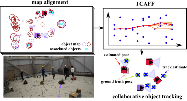
Existing multi-view MOT works often do not address the problem of uncertain localization and instead focus on scenarios with static, calibrated sensors [5, 4, 6] or moving sensors where relative sensor poses are known [7, 8]. However, when MOT is performed onboard mobile robots, instantaneous frame alignment is difficult to achieve for two main reasons. First, robots often operate in environments where global pose knowledge is not available (e.g., indoors or GPS-denied environments), meaning local coordinate frames must be aligned by other methods like pairwise matching of perception information. Second, a robot’s state estimate in its own local frame is susceptible to drift since it must rely only on chained relative pose information from methods like wheel odometry or visual-inertial odometry (VIO). In instances of mobile, multi-view MOT, small amounts of localization error can result in large inaccuracies of the team’s understanding of the dynamic objects in the scene, necessitating methods for real-time frame alignment.

Our previous work [9] (renamed here as MOTLEE-ICP) showed that maps of static objects can be used to realign robot coordinate frames at regular intervals using Iterative Closest Point (ICP) [10] to periodically correct for localization drift. Aligning sparse object maps enables robots to perform frame alignment even when a scene has been observed from very different viewpoints, a scenario in which traditional frame alignment methods (e.g., visual-feature-based place recognition) often fail [11]. Additionally, sparse object maps are more efficient in communication and computation than denser environment representations. However, since ICP performs a local search, [9] was limited to correcting for small errors in localization drift and struggled to recover from incorrect frame alignments. Additionally, since ICP depends on an initial guess [10] for aligning frames, [9] could not be used in cases in which no initial information about relative poses existed (e.g., robots starting in different locations).

This new work, Multiple Object Tracking with Localization Error Elimination (MOTLEE), demonstrates that collaborative MOT can be performed without any initial knowledge of the poses of neighboring robots using our method for no-initial-guess frame alignment. This is achieved by extending and enhancing our previous method [9] in several ways. First, we address the long-standing problem with object-based mapping in robotics that requires an image detection network to be trained to detect certain objects (e.g., doors, chairs, or cones) [9, 12, 13, 14], which requires significant overhead and only allows mapping to perform in environments with a sufficient quantity of pre-trained objects. We follow the works of [15, 16] in leveraging the open-set image segmenter FastSAM [17] for creating maps of generic objects. Additionally, we develop a Temporally Consistent Alignment of Frames Filter (TCAFF) to reject incorrect putative frame alignments and distinguish which frame alignment is correct when multiple alignments seem likely, which is challenging in geometrically ambiguous scenarios such as the ones of interest here. TCAFF uses a modified version of CLIPPER [18, 19] to extract potential map alignments and leverages concepts from Multiple Hypothesis Tracking (MHT) [20, 21, 22] for constructing frame alignment hypothesis trees. TCAFF then determines that a frame alignment is correct only when a hypothesis tree branch demonstrates high temporal consistency. In summary, this work presents several extensions and improvements to MOTLEE-ICP [9] including:

• Object mapping is performed using FastSAM [17] to segment generic objects, enabling MOTLEE to operate in more general environments.

• Frame alignment is performed without needing initial alignment using the new algorithm called TCAFF.

• Incorrect map alignments are rejected and frames can be aligned after long periods without successful alignments using TCAFF.

• A series of new and more challenging hardware experiments demonstrate MOTLEE’s ability to perform frame alignment and collaborative MOT.

With these enhancements, we present MOTLEE with the following overall contributions:

1. A frame alignment filter using a multiple hypothesis framework that leverages temporal consistency to align robot frames without any initial guess, resulting in an average frame alignment accuracy of $0.43\text{\,}\mathrm{m}$ and $2.3\text{\,}\mathrm{d}\mathrm{e}\mathrm{g}$ compared to $3.3\text{\,}\mathrm{m}$ and $37\text{\,}\mathrm{d}\mathrm{e}\mathrm{g}$ of MOTLEE-ICP [9], even when MOTLEE-ICP is given the true initial alignment.

2. A distributed system for performing collaborative MOT onboard mobile robots by handling localization uncertainty and aligning robot frames using local maps.

3. Hardware demonstrations of MOT performed onboard four mobile robots with unknown relative poses in an environment with six pedestrians to be tracked. In addition, we release the hardware dataset and code.

II Related Work

Collaborative MOT has attracted recent research attention as it offers many benefits over single-view MOT, including the ability to sense otherwise occluded objects. However, collaborative MOT adds the additional challenge of determining how to associate and fuse object detections from different views [1]. In this section, we discuss recent research addressing these problems in collaborative MOT.

II-A Collaborative MOT

Collaborative MOT can be centralized [23, 24] or distributed [7, 25, 5, 6, 26]. In a centralized system, all measurement information is sent from robots to a central server, which fuses the measurement information and handles data association with access to all measurement and track information at once. In distributed systems, agents share measurement and estimation information directly with neighbors in their communication network and track estimates are computed collaboratively and in a distributed way.

Because track state information is often one of the biggest informers in cross-view data association, many works consider performing collaborative MOT with known relative sensor pose. The Multi-Target Multi-Camera Tracking (MTMCT) community often focuses on solving a maximum a posteriori optimization problem on a set of recorded videos offline to jointly optimize track estimates over all time [27, 24, 23, 4]. Methods for fusing static sensor information include tracking in the 2D image plane and then associating 2D tracks across views [27, 23], associating detections based on projected 3D locations [5, 4], and using learning based ReID features [23, 5].

Conversely, in a mobile robot scenario, robots require real-time knowledge about the whereabouts of moving objects in their environment (i.e., optimizing objects’ tracks using recorded videos does not suffice). Real-time object tracking onboard moving sensors is commonly approached by incrementally estimating objects’ states as new detections are made. Ong et al. [28] proposed a decentralized particle filtering approach for tracking onboard multiple flight vehicles using global localization information from GPS for vehicles. Shorinwa et al. [7] presented a distributed target tracking method based on consensus ADMM for use on autonomous cars with ground truth localization.

II-B Collaborative MOT with Unknown Localization

Because teams of robots are necessarily going to experience localization drift in their ego-pose estimates, robots cannot accurately share track information with their neighbors in a common coordinate frame without some method to compensate for drift. Recent simultaneous localization and mapping (SLAM) research, has resulted in powerful distributed optimization techniques to accurately rectify the trajectories of multi-robot systems using a combination of single-robot odometry and visual loop closure [29, 30], however the optimization time generally required to achieve consistent frame alignment in standard collaborative SLAM makes its use ill-suited for robotics problems where real-time frame alignment information is required, like collaborative MOT.

To address this, recent work has begun to investigate simultaneous localization and object tracking [31, 32, 33, 34, 35]. Tian et al. [31] introduce a method for performing simultaneous SLAM and MOT on mobile agents with LiDAR sensors by performing data association on objects using similarity scoring on a sliding window of object tracks. Ahmad et al. [36] formulated a joint, collaborative MOT and localization problem as a pose graph optimization for robot soccer. They make the limiting assumption of known data association of measurements with static landmarks and tracked dynamic objects. Taghavi et al. [34] introduced a method for estimating static sensor bias in a multisensor MOT framework in a centralized system. Dames [35] proposed a distributed MOT algorithm based on random finite sets (RFS) and the probability hypothesis density (PHD) with the assumption that localization uncertainty is constant everywhere along the robot’s path. In contrast, MOTLEE uses TCAFF, a multiple hypothesis frame alignment filter, to determine the correct alignment of robot coordinate frames using temporally consistent frame alignment measurements.

III Multi-Robot Frame Alignment

Coordinated, multi-robot tasks require each robot to know the transformations to their neighboring robots’ coordinate frames for collaboration about perceived information. Additionally, a robot must track its own pose within a local frame, which is usually referred to as the odometry frame. We write the $i$-th robot’s pose in its own odometry frame $\mathcal{F}_{\text{odom}_{i}}$ at time $k$ as $\mathbf{T}^{\text{odom}_{i}}_{\text{r}_{i}}(k)$. Since the robot’s pose estimate can be susceptible to drift, we also consider the robot’s pose in a world frame, $\mathbf{T}^{\text{world}}_{\text{r}_{i}}(k)$. Because of drift, the transform between the two coordinate frames, $\mathbf{T}^{\text{odom}_{i}}_{\text{world}}(k)$, may not remain static. We formulate frame alignment as the problem of computing the relative transform between two robots’ odometry frames $\mathbf{T}^{\text{odom}_{i}}_{\text{odom}_{j}}$, which can be used to express spatial information in neighboring robots’ frames.

III-A Map Alignment

We perform frame alignment, finding $\mathbf{T}^{\text{odom}_{i}}_{\text{odom}_{j}}(k)$, by creating sparse maps of recently observed objects in the environment and then aligning the maps of pairs of robots as shown in Fig. 1. The map of each robot is denoted as $\mathcal{M}_{i}$ and is composed of objects represented by their width $w$, height $h$, time since the object was last seen $\ell$, and centroid position $p^{\text{odom}_{i}}$ expressed in $\mathcal{F}_{\text{odom}_{i}}$. To ensure that drifted parts of robot $i$’s map do not affect the estimated $\mathbf{T}^{\text{odom}_{i}}_{\text{odom}_{j}}(k)$, an object is only included in $\mathcal{M}_{i}$ if $\ell<\kappa$, where $\kappa$ is a tuneable parameter based on how fast drift is expected to be incurred.

Maps of recently observed objects are shared with neighboring robots at a regular rate, and frame alignment is performed by treating the alignment of centroids as a point registration problem. As shown in Algorithm 1, we make modifications to the standard CLIPPER method [18, 19] to perform robust global data association between points. CLIPPER solves point registration by formulating the problem as a graph optimization and leveraging geometric consistency to reject outlier associations. First, a consistency graph $\mathcal{G}$ is formed where the nodes $a_{p}$ are putative associations between a point in the first map $p_{i}$ and a point in the second $p_{j}$. Weighted edges exist between nodes if two associations are consistent with each other. This is determined by using a distance measurement, $d(a_{p},a_{q})=\left\lvert\,\|p_{i}-q_{i}\|-\|p_{j}-q_{j}\|\,\right\rvert$. If $d(a_{p},a_{q})<\epsilon$, a weighted edge is added to the graph $\mathcal{E}_{p,q}=s(a_{p},a_{q})$, where $s$ is a function that maps the similarity of two associations to a score $\in[0,1]$. Finally, the edges of the graph are used to create a weighted affinity matrix ${\mathbf{M}}$ where ${\mathbf{M}}_{p,q}=s(a_{p},a_{q})$, and a continuous relaxation of the following problem is optimized

$$\begin{split}\underset{{\mathbf{u}}\in\{0,1\}^{n}}{\max}&\frac{{\mathbf{u}}^{\top}{\mathbf{M}}{\mathbf{u}}}{{\mathbf{u}}^{\top}{\mathbf{u}}}.\\ \text{subject to}\quad&u_{p}u_{q}=0\;\text{if}\;{\mathbf{M}}_{p,q}=0,\;\forall_{p,q},\end{split}$$ (1)

where the elements of ${\mathbf{u}}$ indicate whether an association has been kept as an inlier association. See [19] for more details.

By creating a point cloud from centroids of mapped objects, CLIPPER can be leveraged to form associations between objects within each map, as done in [15], without any initial frame alignment knowledge. We form the initial putative associations given to CLIPPER by only including correspondences that would associate objects with similar widths and heights in both maps to help keep the optimization small enough to be solved in real-time. After objects in each map have been associated, we align the two maps using a weighted Arun’s method [37], where weights are assigned between two objects $W({\mathbf{o}}_{i},{\mathbf{o}}_{j})=(\ell_{i}\ell_{j})^{-1}$ where $\ell$ is the time since ${\mathbf{o}}$ was last seen. This allows objects that were seen more recently (i.e., can give more up-to-date information about relative robot pose) greater influence in the point registration.

III-B Near Optimal Associations

In practice, these sparse maps often include ambiguities in how they should be aligned due to geometric aliasing (i.e., repetitive object structure), difficulty in representing the object’s true centroid due to occlusion and partial observations, small overlap between the two maps, and high noise level from the coarseness of the map representation. These ambiguities can lead to registration problems that have many local optima whose objective values are numerically similar or even cases where the global optimum does not necessarily correspond to correct data associations. Additionally, an alignment between two object maps can still be found even if the maps belong to non-overlapping areas, so a method for rejecting incorrect frame alignments is needed. A heuristic approach can be taken, such as requiring a certain number of associated objects to consider a frame alignment [38], but this requires making assumptions about the expected abundance of objects to be mapped in the environment and may still result in finding incorrect frame alignments or rejecting correct alignments that do not meet the minimum number of associations.

Instead, we propose a multi-hypothesis approach to address these ambiguities. Our method considers different possible alignments of object maps and finds the most likely alignment leveraging consistency of alignments over time. The first step in this process is finding object-to-object associations that are correct but that may be sub-optimal according to (1). To do this, we develop an algorithm to extract multiple near optima from CLIPPER, shown in Algorithm 1.

Algorithm 1 Multiple Near Optima (MNO) CLIPPER

1:Input affinity matrix ${\mathbf{M}}\in[0,1]^{m\times m}$ of consistency graph $\mathcal{G}$

2:Output ${\mathcal{Y}}$ Set of near-optimal transformation meas. of $\mathbf{T}^{\text{odom}_{i}}_{\text{odom}_{j}}$

3:$\mathcal{Y}$ = {}

4:for $n\in 1:N$ do

5:    inlier_associations $\leftarrow$ CLIPPER(${\mathbf{M}}$)

6:    $\mathbf{T}^{\text{odom}_{i}}_{\text{odom}_{j}}\leftarrow\texttt{aruns\_method}(\texttt{inlier\_associations})$

7:    $\mathcal{Y}\leftarrow\mathcal{Y}+\{{{\mathbf{T}}}^{\text{odom}_{i}}_{\text{odom}_{j}}\}$

8:    for $p\in\texttt{inlier\_associations}$ do

9:         for $q\in\texttt{inlier\_associations}$ do

10:             ${\mathbf{M}}_{p,q}\leftarrow 0$              

To search for nearly optimal associations, we initially run the standard CLIPPER, which gives a single set of associations which is often the globally optimal solution to equation (1). Then, elements of the affinity matrix ${\mathbf{M}}$ that were selected by the previous solution are set to 0 to force CLIPPER to find a new set of associations that does not include any of the previously selected associations, which thus yields a new set of nearly optimal associations. This is repeated for a set number of iterations, $N$.

III-C Multiple Hypothesis Formulation

We construct TCAFF, a frame alignment filter for finding map alignments that are consistent over time. This formulation considers different associations of incoming frame alignment measurements and is inspired by MHT [21, 20] which is typically used for assisting with the data association of object detections to tracked object states in the MOT community. Instead, we apply similar concepts to determine when a sequence of frame alignments represents correctly associated map objects between a pair of robots. The goal of TCAFF is at each timestep to take several potential frame alignments, each referred to as frame alignment measurement $\mathbf{{\mathbf{y}}}_{k}\in\mathcal{Y}_{k}$, and produce a filtered frame alignment estimate $\mathbf{{\mathbf{s}}}_{k}$.

For simplicity, we first assume an initial frame alignment guess, $\mathbf{T}^{\text{odom}_{i}}_{\text{odom}_{j}}(k_{0})$. At each timestep $k$, robot $i$ gets many potential frame alignments from MNO-CLIPPER. However, because of map alignment ambiguity or lack of overlapping information (i.e., robots $i$ and $j$ are not mapping any common objects), there exists only one or zero correct frame alignment measurements. By observing these measurements over time, the most likely sequence corresponding to the true frame alignment can be determined. The selected measurements are then filtered to obtain an accurate frame alignment estimate.

This problem can be expressed as a more general maximum a posteriori (MAP) estimation problem of selecting the measurement variables that best fit the model

$$\begin{split}\underset{\begin{subarray}{c}\mathbf{{\mathbf{y}}}_{1}\in\mathcal{Y}_{1},...,\mathbf{{\mathbf{y}}}_{K}\in\mathcal{Y}_{K}\end{subarray}}{\text{arg\,max}}&\quad{p\left(\mathbf{{\mathbf{s}}}_{K}|\,\mathbf{{\mathbf{y}}}_{1},...,\mathbf{{\mathbf{y}}}_{K}\right)}\\ \text{s.t.}&\quad\mathbf{{\mathbf{s}}}_{0}=\mathbf{{\mathbf{s}}}(k_{0}),\\ &\quad\mathbf{{\mathbf{s}}}_{k+1}=\texttt{kalman\_update}(\mathbf{{\mathbf{s}}}_{k},\mathbf{{\mathbf{y}}}_{k}),\end{split}$$ (2)

This formulation can be used in other applications where temporal consistency can be used to give extra information in ambiguous scenarios, but for our specific use case of estimating a frame alignment, we use $\mathbf{{\mathbf{s}}}_{k}$ and $\mathbf{{\mathbf{y}}}_{k}$ as parameterizations of 2D frame alignments $\mathbf{T}^{\text{odom}_{i}}_{\text{odom}_{j}}$ where $\mathbf{{\mathbf{s}}}_{k}={[x,y,\theta]}^{\top}$.

We represent $\mathbf{{\mathbf{s}}}_{k}$ and $\mathbf{{\mathbf{y}}}_{k}$ as Gaussian random variables, which allows us to rewrite equation (2) as

$$\underset{\mathbf{{\mathbf{y}}}_{1:K}}{\text{arg\,max}}\quad\prod_{k=1}^{K}\frac{\exp\left(-\frac{1}{2}\|\mathbf{{\mathbf{y}}}_{k}-{\mathbf{H}}\mathbf{{\mathbf{s}}}_{k}\|^{2}_{\mathbf{S}_{k}}\right)}{\sqrt{(2\pi)^{d_{\mathbf{{\mathbf{y}}}}}\left|\mathbf{S}_{k}\right|}}.$$ (3)

where $d_{\mathbf{{\mathbf{y}}}}$ is the dimension of the measurement vector, ${\mathbf{H}}$ is the measurement matrix, ${\mathbf{S}}_{k}={\mathbf{H}}{\mathbf{P}}_{\mathbf{{\mathbf{s}}}}{\mathbf{H}}^{\top}+{\mathbf{R}}_{\mathbf{{\mathbf{y}}}}$ is the innovation covariance matrix, ${\mathbf{P}}_{\mathbf{{\mathbf{s}}}}$ is the estimate covariance resulting from the Kalman Filter, and ${\mathbf{R}}_{\mathbf{{\mathbf{y}}}}$ is the measurement covariance. Taking the negative logarithm of equation (3) yields

$$\begin{split}\underset{\mathbf{{\mathbf{y}}}_{1:K}}{\text{arg\,min}}\quad\sum_{k=1}^{K}\frac{1}{2}\left({d_{\mathbf{{\mathbf{y}}}}}\log(2\pi)+\|\mathbf{{\mathbf{y}}}_{k}-{\mathbf{H}}\mathbf{{\mathbf{s}}}_{k}\|^{2}_{\mathbf{S}_{k}}+\right.\left.\log(|\mathbf{S}_{k}|)\right).\end{split}$$ (4)

If there is no measurement at time $k$ (i.e., ${\mathbf{{\mathbf{y}}}_{k}=\text{None}}$), we use a probability of no measurement $p_{\text{NM}}$ resulting in

$$\begin{split}\underset{\mathbf{{\mathbf{y}}}_{1:K}}{\text{arg\,min}}\,\sum_{k=1}^{K}\begin{cases}\frac{1}{2}\left(\|\mathbf{{\mathbf{y}}}_{k}-{\mathbf{H}}\mathbf{{\mathbf{s}}}_{k}\|^{2}_{\mathbf{S}_{k}}+\log(|\mathbf{S}_{k}|)\right),&\mathbf{{\mathbf{y}}}_{k}\in\mathcal{Y}_{k}\\ -{\log}(p_{\text{NM}})-\frac{1}{2}{d_{\mathbf{{\mathbf{y}}}}}\log(2\pi),&\mathbf{{\mathbf{y}}}_{k}=\text{None}.\end{cases}\end{split}$$ (5)

We solve this optimization problem with a multi-hypothesis approach to find the correct frame alignment from a set of potentially incorrect frame alignment measurements. Thus, the robots use TCAFF to delay hard data association decisions until adequate information is gained and frame alignment measurements can be evaluated for temporal consistency.

III-D Frame Alignment Filter

((a))

((b))

((c))

Figure 2: Visualization of TCAFF multiple hypothesis process. (a) A new set of measurements is computed. (b) Leaf nodes are extended by applying Kalman Filter updates with candidate measurements. (c) Window is slid forward and unlikely branches are pruned.

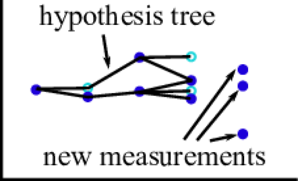
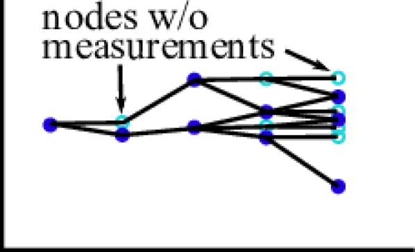
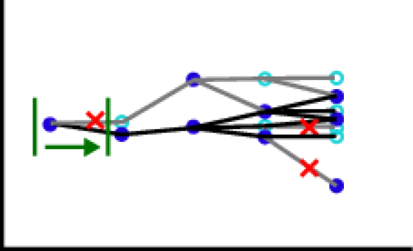
Finding optimal frame alignments in (5) amounts to evaluating measurements as branches of a tree. At the root of the tree is the initial state estimate $\hat{\mathbf{{\mathbf{s}}}}_{0}$ and covariance ${\mathbf{P}}_{\mathbf{{\mathbf{s}}}_{0}}$. The root is connected to one or more children by different edges, each child representing an estimate $\hat{\mathbf{{\mathbf{s}}}}_{1}$ and each edge representing a selected measurement $\mathbf{{\mathbf{y}}}_{1}$. As leaves of the tree $\hat{\mathbf{{\mathbf{s}}}}_{k}$ are added, the optimal estimate $\hat{\mathbf{{\mathbf{s}}}}^{*}_{k}$ can be found by selecting the sequence of measurements resulting in the minimum objective value (5). Because the objective value of a node’s child is the sum of its own objective value and an additional cost, computation can be saved by reusing the node’s pre-computed cost when adding children.

An update step is illustrated in Fig. 2. First, new measurements $\mathcal{Y}_{k}$ are obtained from MNO CLIPPER. Next, a gating is performed for each leaf node $\hat{\mathbf{{\mathbf{s}}}}_{k}$ and $\mathbf{{\mathbf{y}}}_{k}$ that prohibits adding nodes with high cost values (i.e., highly unlikely measurements), helping keep computation requirements low. A Kalman filter update [39] is then performed between each associated node and measurement to compute $\hat{\mathbf{{\mathbf{s}}}}_{k+1}=\texttt{kalman\_update}(\mathbf{{\mathbf{s}}}_{k},\mathbf{{\mathbf{y}}}_{k})$, and $\hat{\mathbf{{\mathbf{s}}}}_{k+1}$ is added to the tree as a new leaf node.

Finally, because this hypothesis tree approach is exponential in complexity, pruning must be employed to keep computation manageable. We employ a “sliding window” and “max branches” pruning approach [22]. For a sliding window of length $W$, all branches $\mathbf{{\mathbf{s}}}_{k-W}$ that do not have the leaf node $\mathbf{{\mathbf{s}}}_{k}^{*}$ as a descendant are pruned, leaving only a single $\mathbf{{\mathbf{s}}}_{k-W}$ node, which becomes the root of the new window-bound hypothesis tree. Then, for a maximum number of branches $B$, only the $B$ most optimal leaves are kept and the rest are pruned.

To apply our TCAFF approach to a scenario where no initial $\mathbf{{\mathbf{s}}}_{0}$ exists, we introduce a sliding window method for exploring possible initial frame alignments $\mathbf{{\mathbf{s}}}_{0}$. At each timestep $k$, each measurement $\mathbf{{\mathbf{y}}}_{k-W}$ is used to initialize the root of a new exploring tree. The measurements in $\mathcal{Y}_{k-W+1}$, …, $\mathcal{Y}_{k}$ are all added to each of the exploring trees and the optimal $\mathbf{{\mathbf{s}}}^{*}_{k}$ from all of the exploring trees is selected and compared against a threshold $\tau_{\text{align}}$ to determine whether to initialize a “main” tree with the corresponding root at $\mathbf{{\mathbf{s}}}_{k-W}$. Until a main tree has been selected, the method declares that no frame alignment estimate can be found. Similarly, a mechanism is needed to remove a main tree and go back to the exploring phase if it becomes unlikely that the main tree is correct. We return to the exploring phase if enough time has passed during which no measurements have been added to the optimal leaf node. This method allows robots to leverage temporal consistency (i.e., the fact that a correct frame alignment estimate should produce many consistent measurements over time) to reject incorrect measurements and align frames with no initial guess.

IV Collaborative MOT

Having identified pairwise relative transformations that align robot coordinate frames using our TCAFF approach, robots collaboratively track objects using the method presented in this section. The objective of MOT is to estimate $\mathbf{x}(k)$, the state of each dynamic object in an environment at time $k$, using measurements $\mathbf{z}(k)$ and modeled by a discrete-time linear dynamic system

$$\mathbf{x}(k+1)=\mathbf{A}\mathbf{x}(k)+\mathbf{w}(k),\quad\mathbf{z}(k)=\mathbf{H}\mathbf{x}(k)+\mathbf{v}(k),$$ (6)

where $\mathbf{A}$ and $\mathbf{H}$ are the transition and measurement matrices, respectively, and $\mathbf{w}(k)\sim\mathcal{N}(0,\mathbf{Q}(k))$ and $\mathbf{v}(k)\sim\mathcal{N}(0,\mathbf{R}(k))$ are zero-mean independent Gaussian process and measurement noise with covariance matrices $\mathbf{Q}$ and $\mathbf{R}$, respectively. Each robot keeps a local bank of state estimates of dynamic objects, $\hat{\mathbf{x}}(k)$, also referred to as tracks.

We adopt the distributed track management system of [5] to handle sharing track information between robots, and shared track information is incorporated using the Kalman Consensus Filter (KCF) [40, 41], as described in the remainder of this section.

At each timestep, each robot obtains dynamic object measurements ${\mathbf{z}}(k)$ from sensory input and then executes three tasks to collaboratively track objects: (1) perform local data association between new measurements and tracks in robot $i$’s local bank, (2) share updated KCF information with neighboring robots, and (3) perform KCF updates.

IV-A Local Data Association

Local Data Association (LDA) is the process of determining for each measurement whether it should be assigned to an existing track or whether it belongs to a new object that is not being tracked. This association decision is made by evaluating the negative logarithm of the matching likelihood (NLML) [42] between each measurement $\mathbf{z}(k)$ and each existing track prediction as

$$\begin{split}\text{NLML}(\hat{\mathbf{x}}^{+}(k),\mathbf{z}(k+1))=\;&\|\mathbf{z}(k)-{\mathbf{H}}\hat{\mathbf{x}}^{+}(k)\|_{{\mathbf{S}}}^{2}\\ &~{}~{}+d\log 2\pi+\log\left(|{\mathbf{S}}|\right).\end{split}$$ (7)

where $\hat{\mathbf{x}}^{+}(k)={\mathbf{A}}\hat{\mathbf{x}}(k)$, $d_{\mathbf{z}}$ is the dimension of the measurement vector, and ${\mathbf{S}}={\mathbf{H}}{\mathbf{P}}{\mathbf{H}}^{\top}+{\mathbf{R}}$ is the innovation covariance. We solve the LDA using a global nearest neighbor (GNN) approach [1] where the measurement-to-track association is formulated as a linear assignment problem and the NLML of each association is minimized using the Hungarian algorithm [43]. We apply a gate, $\tau$, such that an $\hat{\mathbf{x}}(k)$ cannot be matched with a $\mathbf{z}(k)$ if $\text{NLML}(\hat{\mathbf{x}}^{+}(k),\mathbf{z}(k+1))>\tau$. Any unmatched measurements are set aside as part of a trial database where after $\nu$ sequential measurements, the trial track is accepted as a new track.

IV-B Information Sharing

Once measurements and tracks have been associated, robot $i$ sends the message containing KCF update information to each neighboring robot $j$. It is important to note that because the robots’ coordinate frames differ, quantities expressed in $\mathcal{F}_{\text{odom}_{i}}$ must be transformed into $\mathcal{F}_{\text{odom}_{j}}$ and the uncertainty associated with that transformation must also be reflected in the uncertainty associated with shared measurements and state estimates. We use the notation $p^{j}_{i}$ to designate a quantity $p$ that originated from robot $i$, and is now expressed in robot $j$’s odometry frame $\mathcal{F}_{\text{odom}_{j}}$ using the estimated frame transformation $\mathbf{T}^{\text{odom}_{i}}_{\text{odom}_{j}}$. For each track, the information $(\texttt{ID},\hat{\mathbf{x}}^{j+}_{i},{\mathbf{u}}^{j}_{i},{\mathbf{U}}^{j}_{i})$ is shared, where ID is a unique ID for the track, ${\mathbf{u}}$ and ${\mathbf{U}}$ are the information vector and information matrix associated with the track respectively. The information vector and matrix are formed with

$$\mathbf{u}^{j}_{i}=\mathbf{H}^{\top}(\mathbf{R}^{j}_{i})^{-1}\mathbf{z}^{j}_{i},\quad\mathbf{U}^{j}_{i}=\mathbf{H}^{\top}(\mathbf{R}^{j}_{i})^{-1}\mathbf{H},$$ (8)

where ${\mathbf{R}}^{j}_{i}$ is computed by propagating the measurement covariance through the uncertain frame transformation $\mathbf{T}^{\text{odom}_{i}}_{\text{odom}_{j}}(k)$, which will be discussed in Section IV-D.

IV-C Kalman Consensus Filter

Once robot $i$ has received messages from each of its neighbors, the information is aggregated as

$$\mathbf{y}^{i}=\sum_{j\in\mathcal{N}_{i}\cup i}\mathbf{u}^{i}_{j},\qquad\mathbf{Y}^{i}=\sum_{j\in\mathcal{N}_{i}\cup i}\mathbf{U}^{i}_{j},$$ (9)

where $\mathcal{N}_{i}$ represents each neighbor of robot $i$. Track estimates are then obtained by fusing together all shared information using the KCF update,

$$\begin{aligned} \hat{\mathbf{x}}^{i}(k+1)&=\hat{\mathbf{x}}^{i+}_{i}(k)+\mathbf{M}^{i}(k)\bigl{[}\mathbf{y}^{i}(k)-\mathbf{Y}^{i}(k)\hat{\mathbf{x}}^{i+}_{i}(k)\bigr{]}\\ &\quad+\frac{\mathbf{M}^{i}(k)}{1+\|\mathbf{M}^{i}(k)\|}\sum_{j\in\mathcal{N}_{i}}\bigl{(}\hat{\mathbf{x}}^{i+}_{j}(k)-\hat{\mathbf{x}}^{i+}_{i}(k)\bigr{)},\end{aligned}$$ (10)

where ${\mathbf{M}}^{i}(k)=({{\mathbf{P}}^{i}(k)}^{-1}+{{\mathbf{Y}}^{i}(k)})^{-1}$ is the Kalman gain in information form, and ${\mathbf{P}}^{i}(k)$ is the estimation covariance. Finally, ${\mathbf{P}}^{i}(k)$ is updated with ${\mathbf{A}}{\mathbf{M}}^{i}(k){\mathbf{A}}^{\top}+{\mathbf{Q}}^{i}(k)$.

IV-D Uncertainty Propagation

To share the measurement $\mathbf{z}^{i}_{i}$, robot $i$ must transform $\mathbf{z}^{i}_{i}$ into the frame $\mathcal{F}_{\text{odom}_{j}}$, and the frame alignment uncertainty ${\mathbf{P}}_{\mathbf{{\mathbf{s}}}}$ must be properly incorporated with the initial measurement uncertainty ${\mathbf{R}}^{i}_{i}$. We parameterize the frame alignment and its associated uncertainty using Euler angles, following Smith, Self, and Cheeseman (SSC) [44]. Then, ${\mathbf{R}}^{j}_{i}$ can be found by combining the uncertainty in the object measurement and the frame alignment with

$${\mathbf{R}}^{j}_{i}={\mathbf{I}}_{d_{\mathbf{z}}\times d_{\mathbf{{\mathbf{y}}}}}{\mathbf{J}}{\mathbf{P}}_{\mathbf{{\mathbf{s}}}}{\mathbf{J}}^{\top}{\mathbf{I}}_{d_{\mathbf{z}}\times d_{\mathbf{{\mathbf{y}}}}}^{\top}+{\mathbf{C}}^{\text{odom}_{i}}_{\text{odom}_{j}}{\mathbf{R}}^{i}_{i}({\mathbf{C}}^{\text{odom}_{i}}_{\text{odom}_{j}})^{\top}.$$ (11)

where ${\mathbf{J}}$ is the left half of the Jacobian of the compounding (relative head-to-tail) relation, ${\mathbf{P}}_{\mathbf{{\mathbf{s}}}}$ is the covariance of the current TCAFF frame alignment estimate, and ${\mathbf{C}}^{\text{odom}_{i}}_{\text{odom}_{j}}$ is the right half of the Jacobian of the compounding relation, which is also the rotation matrix component of the frame alignment estimate $\hat{\mathbf{{\mathbf{s}}}}$.

V Experiments

We experimentally evaluate our TCAFF method for aligning coordinate frames in a temporally consistent manner in Sections V-A and V-B. The results from our full collaborative MOTLEE system using TCAFF are shown in Section V-C. Unless otherwise stated, the following parameter values were used for all experiments: $\kappa=20.0$, $\tau=10.0$, $\nu=3$, $p_{\text{NM}}=0.001$, $\tau_{\text{align}}=8.0$, $N=4$, $W=8$, and $B=200$.

V-A Indoor Frame Alignment Experiment

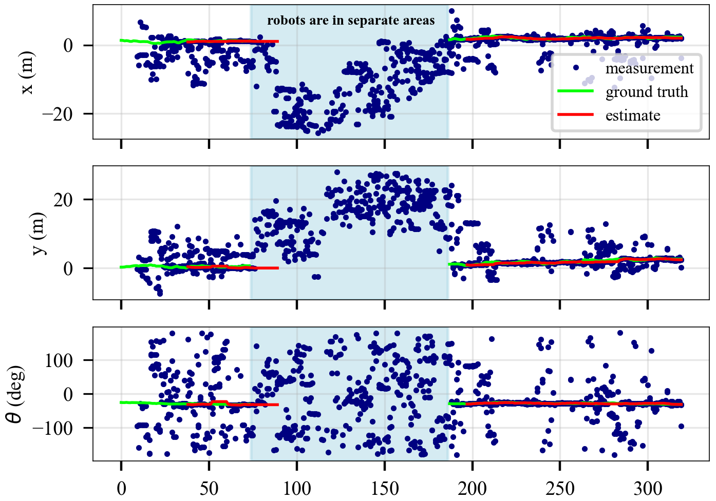
First, we evaluate TCAFF’s ability to estimate the frame alignment between two robots without any initial guess, which requires the ability to distinguish between maps that belong to the same area and maps that result from traveling in non-overlapping areas. Two robots start are initially driven around a $10\times 10\text{\,}\mathrm{m}$ motion-capture room. The robots are equipped with an Intel RealSense T265 Tracking Camera whose onboard VIO is used for ego-pose estimation and an Intel RealSense L515 LiDAR Camera that is used for extracting depths of segments detected by FastSAM. In our experiments, object maps are updated at $10\text{\,}\mathrm{H}\mathrm{z}$ and are shared at $1\text{\,}\mathrm{H}\mathrm{z}$. Each robot’s TCAFF is updated upon the reception of a neighboring robot’s map. Boxes are scattered around the room to represent generic objects that can be detected by the open-set segmentation of FastSAM [17]. Both robots start in the room, and then one robot leaves and accumulates odometry error out-of-view of the other robot before returning to the room for the remainder of the experiment.

In Fig. 3 the frame alignment results from this experiment demonstrate that the robots accurately estimate frame alignments when maps overlap at the start and end of the experiment. Additionally, the robots correctly recognize that potential alignments in the middle of the run do not exhibit temporal consistency and should not be incorporated into the frame alignment estimate. During the times when an estimate is made, the robots estimate the relative frame alignments with average translation and rotation errors of $0.35\text{\,}\mathrm{m}$ and $1.1\text{\,}\mathrm{d}\mathrm{e}\mathrm{g}$ respectively.

Figure 3: TCAFF is visualized by plotting the frame alignment measurements from MNO-CLIPPER in blue along with the ground truth and TCAFF frame alignment estimate. Each blue dot represents a frame alignment measurement $\mathbf{{\mathbf{y}}}(k)=[x,y,\theta]^{\top}$, with the $x$, $y$, and $\theta$ axes shown in separate plots. TCAFF correctly recognizes when enough temporally consistent measurements are received to verify a correct frame alignment. The ground truth frame alignment disappears in the middle of the run when one robot leaves the VICON room and its ground truth pose is unavailable. While in separate areas, map information is still exchanged, and MNO-CLIPPER can be used to find alignments between the two maps, but TCAFF rejects these temporally inconsistent measurements.

Figure 4: Images from the two robots traveling in opposite directions in the Kimera-Multi dataset [11].

V-B Outdoor Frame Alignment Experiment

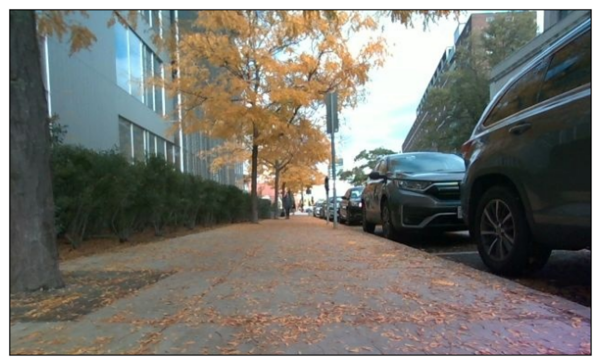
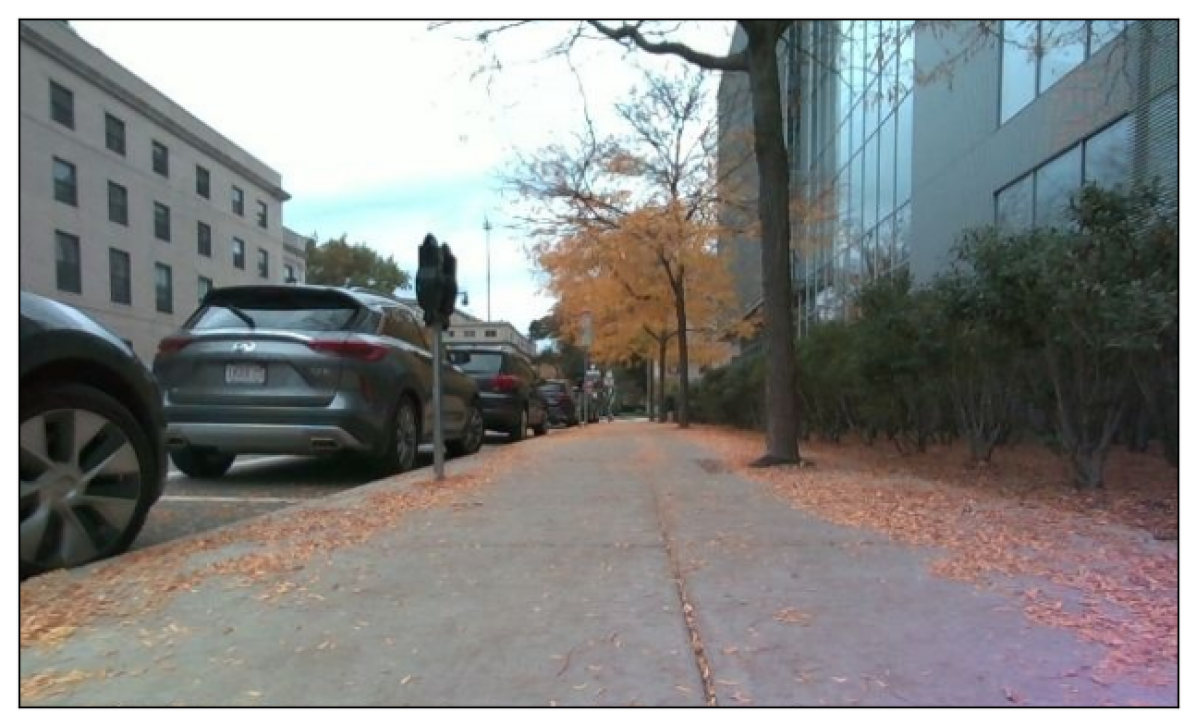
The second experiment uses data collected in the Kimera-Multi outdoor dataset [11] to test our open-set object mapping and TCAFF system in natural outdoor environments. We test our frame alignment method working in two instances, one where robots run parallel to each other along the same path and the other where robots start $50\text{\,}\mathrm{m}$ away from each other and then cross paths. Traditional, image-based loop closure techniques fail to detect that robots cross paths when traveling opposite directions because of the large viewpoint difference as discussed in [11]. Images from the two robots’ runs are shown in Fig. 4 and the average and standard deviation of frame alignment errors are shown in Table I. The translation and rotation errors are computed as the difference between TCAFF’s estimate and the ground truth frame alignment, noting that TCAFF’s estimate only occurs after accepting an exploring hypothesis tree. The following parameters are changed in these outdoor experiments: $\kappa=15.0$ and $W=5$. This maintains objects in the map of recently seen objects for less time since odometry drift is worse in these scenarios. We show that our method correctly estimates frame alignments in challenging outdoor scenarios from the Kimera-Multi outdoor dataset, including a scenario where robots only observe the scene from opposite directions as they cross paths.

TABLE I: Kimera-Multi Data Results

	Avg. Translation Error [m]	Avg. Heading Error [deg]
Same direction	$1.01\pm 0.85$	$1.08\pm 0.82$
Opposite directions	$1.63\pm 0.67$	$1.11\pm 0.48$

V-C Full Collaborative MOT Experiment

Finally, we evaluate the full MOTLEE system’s collaborative object-tracking performance onboard robots with unknown localizations. We record and release a dataset of four robots driving autonomously around a motion capture room while six pedestrians walk around in the same space. This multi-robot MOT experiment presents many additional challenges when compared to the dataset recorded in [9], including more pedestrians and robots, robot trajectories that cover the whole motion capture space rather than non-overlapping areas, and the absence of domain-specific objects (e.g., cones) used for creating object maps.

We use the same sensors used in the V-A experiment with the substitution of the Intel RealSense T265 for an Intel RealSense D455 camera attached to the rear of the robot. Kimera-VIO [45] is used for ego-pose estimation and YOLOv7 [46] for person detection. We evaluate the MOT performance using the Multi-Object Tracking Accuracy (MOTA) metric [47]

$$\text{MOTA}=1-\frac{\Sigma_{k}(m(k)+fp(k)+mme(k))}{\Sigma_{k}g(k)},$$ (12)

where $m(k)$ is the number of missed ground truth objects, $fp(k)$ is the number of false positives, $mme(k)$ is the number of mismatches or objects that were reported under a different ID at time $k$ than the ID previously used for that object, and $g(k)$ is the number of ground-truth objects in the scene.

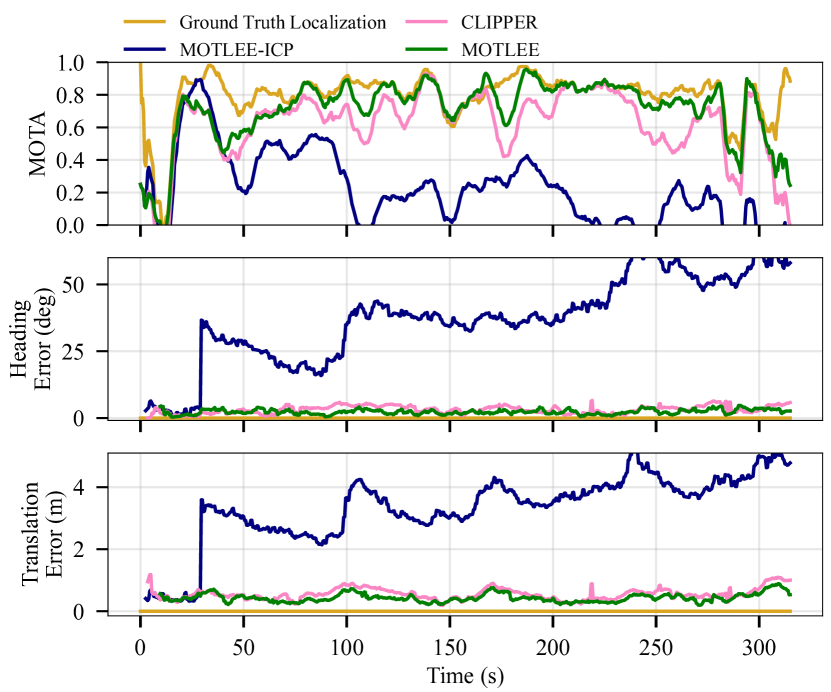
In Fig. 5 we compare the MOTA results of our full MOTLEE system against robots that align frame using MOTLEE-ICP [9], CLIPPER [19], and ground truth frame alignment. Note that only MOTLEE-ICP is given the correct initial frame alignment. In the CLIPPER benchmarks, we accept the association solution from standard CLIPPER as long as a minimum number of objects are associated between the two maps and otherwise reject the alignment, and we show the CLIPPER method’s sensitivity to this parameter. If the required number of associations is low, some incorrect associations are not rejected which hurts the performance of the inter-robot frame alignment and collaborative MOT. Alternatively, a high minimum number of associated objects may be set, but this makes a restrictive assumption about the expected quantity of overlapping objects in the two maps, and can result in many fewer accepted alignments. Our method allows a system to benefit from the best of both worlds, additionally benefiting from alignments that can only be found when using our MNO variation of CLIPPER. With TCAFF, incorrect alignments are rejected and alignments can be found even when the maps have very little overlap.

Figure 5: Comparison of MOTA results. Results for using a single CLIPPER solution that requires a set minimum number of associations are shown for a sweep of different parameter values. TCAFF is able to consider all potential alignments and reject incorrect frame alignments by leveraging temporal consistency, resulting in a higher object tracking accuracy.

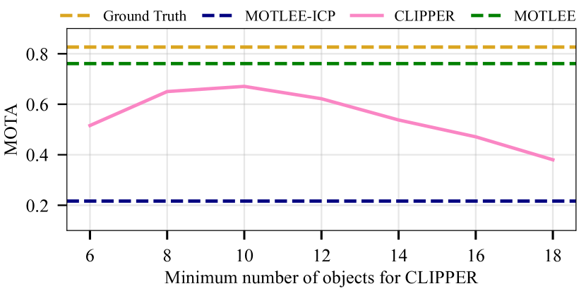
Additionally, we show MOTA over a rolling window and frame alignment results in Fig. 6. MOTLEE achieves a total MOTA of $0.761$, close to the ground-truth MOTA of $0.827$, and achieves an average frame alignment error of $0.43\text{\,}\mathrm{m}$ and $2.3\text{\,}\mathrm{d}\mathrm{e}\mathrm{g}$.

Figure 6: Comparison of object tracking accuracy and frame alignment accuracy in an experiment with four robots tracking six pedestrians. MOTA is computed over a rolling window of $10\text{\,}\mathrm{s}$. MOTLEE using TCAFF for frame alignment is benchmarked against frame alignment from MOTLEE-ICP [9], CLIPPER [19], and ground truth frame alignment. Note that the CLIPPER benchmark rejects any alignments with fewer than $10$ associations since this results in its best MOTA performance as seen in Fig. 5. MOTLEE is able to estimate frame alignments with no initial guess, use frame alignments with few associated objects by leveraging temporal consistency, and collaboratively track objects with accuracy similar to that of robots with ground truth localization.

V-D Computation Time

We have broken up different pieces of the system to evaluate the computation time of the different elements where the mean and standard deviation of computation times are shown in Table II. MNO-CLIPPER and TCAFF must both be performed for each neighboring robot. Each of the tasks listed in Table II can easily be run in parallel for running MOTLEE in real-time.

TABLE II: Timing Analysis [ms]

Mapping (10 Hz)	MOT (10 Hz)	MNO-CLIPPER (1 Hz)	TCAFF (1 Hz)
$13.5\pm 8.0$	$2.2\pm 0.9$	$150.2\pm 45.3$	$18.6\pm 20.5$

VI Conclusion

We presented MOTLEE, a distributed and collaborative MOT method that is applicable in the presence of per-robot and inter-robot localization uncertainty. By leveraging temporal consistency and multiple frame alignment hypotheses, we developed TCAFF, which allows MOTLEE to perform pairwise frame alignments even in the presence of map ambiguity or in settings where no initial frame alignment is known. Although our implementation is specifically aimed at aligning coordinate frames, TCAFF could be used for other state estimation tasks that require rejecting many temporally inconsistent false-positive measurements.

Limitations to our work include a tendency to create cluttered maps due to FastSAM segmenting different parts of an environment that may not be associated with a single object (e.g., segmenting small parts of an object or segmenting multiple objects together depending on the specific image). Additionally, there is a trade-off when using temporal consistency that can result in taking a few seconds to recognize robots are in the same place.

Future work includes demonstrating TCAFF’s ability to be incorporated with other methods for frame alignment (e.g., via visual bag-of-words) and to incorporate additional information into object representation which can be leveraged for associating objects between maps.

References

- [1] Y. Bar-Shalom and X.-R. Li, Multitarget-multisensor tracking: principles and techniques. YBs Storrs, CT, 1995, vol. 19.
- [2] T. Chavdarova, P. Baqué, S. Bouquet, A. Maksai, C. Jose, T. Bagautdinov, L. Lettry, P. Fua, L. Van Gool, and F. Fleuret, “Wildtrack: A multi-camera hd dataset for dense unscripted pedestrian detection,” in IEEE/CVF CVPR, 2018, pp. 5030–5039.
- [3] P. Nguyen, K. G. Quach, C. N. Duong, N. Le, X.-B. Nguyen, and K. Luu, “Multi-camera multiple 3d object tracking on the move for autonomous vehicles,” in IEEE/CVF CVPR, 2022, pp. 2569–2578.
- [4] F. Fleuret, J. Berclaz, R. Lengagne, and P. Fua, “Multicamera people tracking with a probabilistic occupancy map,” IEEE TPAMI, 2007.
- [5] S. Casao, A. Naya, A. C. Murillo, and E. Montijano, “Distributed multi-target tracking in camera networks,” in IEEE ICRA, 2021.
- [6] N. F. Sandell and R. Olfati-Saber, “Distributed data association for multi-target tracking in sensor networks,” in IEEE CDC, 2008.
- [7] O. Shorinwa, J. Yu, T. Halsted, A. Koufos, and M. Schwager, “Distributed multi-target tracking for autonomous vehicle fleets,” in IEEE ICRA, 2020, pp. 3495–3501.
- [8] T. Kroeger, R. Dragon, and L. Van Gool, “Multi-view tracking of multiple targets with dynamic cameras,” in GCPR. Springer, 2014.
- [9] M. B. Peterson, P. C. Lusk, and J. P. How, “Motlee: Distributed mobile multi-object tracking with localization error elimination,” in IEEE/RSJ IROS, 2023, pp. 719–726.
- [10] P. J. Besl and N. D. McKay, “Method for registration of 3-d shapes,” in Sensor fusion IV: control paradigms and data structures, vol. 1611. Spie, 1992, pp. 586–606.
- [11] Y. Tian, Y. Chang, L. Quang, A. Schang, C. Nieto-Granda, J. How, and L. Carlone, “Resilient and distributed multi-robot visual SLAM: Datasets, experiments, and lessons learned,” in IEEE/RSJ IROS, 2023.
- [12] S. L. Bowman, N. Atanasov, K. Daniilidis, and G. J. Pappas, “Probabilistic data association for semantic slam,” in IEEE ICRA, 2017.
- [13] L. Nicholson, M. Milford, and N. Sünderhauf, “Quadricslam: Dual quadrics from object detections as landmarks in object-oriented slam,” IEEE Robotics and Automation Letters, vol. 4, no. 1, pp. 1–8, 2018.
- [14] S. Yang and S. Scherer, “Cubeslam: Monocular 3-d object slam,” IEEE Transactions on Robotics, vol. 35, no. 4, pp. 925–938, 2019.
- [15] J. Kinnari, A. Thomas, P. Lusk, K. Kondo, and J. P. How, “Sos-slam: Segmentation for open-set slam in unstructured environments,” arXiv preprint arXiv:2401.04791, 2024.
- [16] K. Kondo, C. T. Tewari, M. B. Peterson, A. Thomas, J. Kinnari, A. Tagliabue, and J. P. How, “Puma: Fully decentralized uncertainty-aware multiagent trajectory planner with real-time image segmentation-based frame alignment,” arXiv preprint arXiv:2311.03655, 2023.
- [17] X. Zhao, W. Ding, Y. An, Y. Du, T. Yu, M. Li, M. Tang, and J. Wang, “Fast segment anything,” arXiv preprint arXiv:2306.12156, 2023.
- [18] P. C. Lusk, K. Fathian, and J. P. How, “CLIPPER: A graph-theoretic framework for robust data association,” in IEEE ICRA, 2021.
- [19] P. C. Lusk and J. P. How, “CLIPPER: Robust Data Association without an Initial Guess,” IEEE Robotics and Automation Letters, pp. 1–8, 2024.
- [20] S. S. Blackman, “Multiple hypothesis tracking for multiple target tracking,” IEEE Aerosp. Electron. Syst. Mag., vol. 19, pp. 5–18, 2004.
- [21] D. Reid, “An algorithm for tracking multiple targets,” IEEE transactions on Automatic Control, vol. 24, no. 6, pp. 843–854, 1979.
- [22] C. Kim, F. Li, A. Ciptadi, and J. M. Rehg, “Multiple hypothesis tracking revisited,” in IEEE ICCV, 2015, pp. 4696–4704.
- [23] E. Ristani and C. Tomasi, “Features for multi-target multi-camera tracking and re-identification,” in IEEE CVF/CVPR, 2018.
- [24] M. Hofmann, D. Wolf, and G. Rigoll, “Hypergraphs for joint multi-view reconstruction and multi-object tracking,” in IEEE/CVF CVPR, 2013.
- [25] L. He, G. Liu, G. Tian, J. Zhang, and Z. Ji, “Efficient multi-view multi-target tracking using a distributed camera network,” IEEE Sensors Journal, vol. 20, no. 4, pp. 2056–2063, 2019.
- [26] A. T. Kamal, J. H. Bappy, J. A. Farrell, and A. K. Roy-Chowdhury, “Distributed multi-target tracking and data association in vision networks,” IEEE T-PAMI, vol. 38, no. 7, pp. 1397–1410, 2015.
- [27] M. Bredereck, X. Jiang, M. Körner, and J. Denzler, “Data association for multi-object tracking-by-detection in multi-camera networks,” in IEEE ICDSC, 2012.
- [28] L.-L. Ong, B. Upcroft, T. Bailey, M. Ridley, S. Sukkarieh, and H. Durrant-Whyte, “A decentralised particle filtering algorithm for multi-target tracking across multiple flight vehicles,” in IEEE/RSJ IROS, 2006.
- [29] Y. Tian, Y. Chang, F. H. Arias, C. Nieto-Granda, J. P. How, and L. Carlone, “Kimera-multi: robust, distributed, dense metric-semantic slam for multi-robot systems,” IEEE Transactions on Robotics, 2022.
- [30] P. Schmuck, T. Ziegler, M. Karrer, J. Perraudin, and M. Chli, “Covins: Visual-inertial slam for centralized collaboration,” in IEEE ISMAR, 2021, pp. 171–176.
- [31] X. Tian, Z. Zhu, J. Zhao, G. Tian, and C. Ye, “Dl-slot: Dynamic lidar slam and object tracking based on collaborative graph optimization,” arXiv preprint arXiv:2212.02077, 2022.
- [32] O. Dagan, T. L. Cinquini, L. Morrissey, K. Such, N. R. Ahmed, and C. Heckman, “Towards decentralized heterogeneous multi-robot slam and target tracking,” arXiv preprint arXiv:2306.04570, 2023.
- [33] A. Ahmad, G. Lawless, and P. Lima, “An online scalable approach to unified multirobot cooperative localization and object tracking,” IEEE transactions on robotics, vol. 33, no. 5, pp. 1184–1199, 2017.
- [34] E. Taghavi, R. Tharmarasa, T. Kirubarajan, Y. Bar-Shalom, and M. Mcdonald, “A practical bias estimation algorithm for multisensor-multitarget tracking,” IEEE T-AES, vol. 52, no. 1, pp. 2–19, 2016.
- [35] P. M. Dames, “Distributed multi-target search and tracking using the phd filter,” Autonomous robots, vol. 44, no. 3-4, pp. 673–689, 2020.
- [36] A. Ahmad, G. D. Tipaldi, P. Lima, and W. Burgard, “Cooperative robot localization and target tracking based on least squares minimization,” in IEEE ICRA, 2013, pp. 5696–5701.
- [37] K. S. Arun, T. S. Huang, and S. D. Blostein, “Least-squares fitting of two 3-d point sets,” IEEE TPAMI, no. 5, pp. 698–700, 1987.
- [38] Y. Tian, K. Liu, K. Ok, L. Tran, D. Allen, N. Roy, and J. P. How, “Search and rescue under the forest canopy using multiple uavs,” IJRR, vol. 39, no. 10-11, pp. 1201–1221, 2020.
- [39] R. E. Kalman and R. S. Bucy, “New results in linear filtering and prediction theory,” 1961.
- [40] R. Olfati-Saber, “Distributed kalman filtering for sensor networks,” in IEEE CDC, 2007, pp. 5492–5498.
- [41] ——, “Kalman-consensus filter: Optimality, stability, and performance,” in IEEE CDC, 2009, pp. 7036–7042.
- [42] J.-L. Blanco, J. González-Jiménez, and J.-A. Fernández-Madrigal, “An alternative to the mahalanobis distance for determining optimal correspondences in data association,” IEEE T-RO, vol. 28, no. 4, 2012.
- [43] H. W. Kuhn, “The hungarian method for the assignment problem,” Naval Research Logistics Quarterly, vol. 2, no. 1-2, pp. 83–97, 1955.
- [44] R. C. Smith and P. Cheeseman, “On the representation and estimation of spatial uncertainty,” IJRR, vol. 5, no. 4, pp. 56–68, 1986.
- [45] A. Rosinol, M. Abate, Y. Chang, and L. Carlone, “Kimera: an open-source library for real-time metric-semantic localization and mapping,” in IEEE ICRA, 2020, pp. 1689–1696.
- [46] C.-Y. Wang, A. Bochkovskiy, and H.-Y. M. Liao, “Yolov7: Trainable bag-of-freebies sets new state-of-the-art for real-time object detectors,” in IEEE/CVF CVPR, 2023, pp. 7464–7475.
- [47] K. Bernardin and R. Stiefelhagen, “Evaluating multiple object tracking performance: the CLEAR MOT metrics,” EURASIP Journal on Image and Video Processing, vol. 2008, pp. 1–10, 2008.