In-depth analysis of LISA Pathfinder performance results:
time evolution, noise projection, physical models, and implications for LISA

Abstract

We present an in-depth analysis of the LISA Pathfinder differential acceleration performance over the entire course of the mission science operations, spanning about 500 days. We show that the frequency-independent Brownian noise level, detected in the acceleration amplitude spectral density (ASD), for frequencies $f\gtrsim$1\text{\,}\mathrm{m}\mathrm{H}\mathrm{z}$$, in all measurement runs, has been evolving consistently with the decaying pressure due to the outgassing of a single gaseous species, with an activation temperature of $(7.0\pm 0.2)\,\text{kK}$. In excess to the Brownian noise, the acceleration ASD always shows a sub-mHz tail which is reasonably well fit, between $f=$36\text{\,}\mathrm{\SIUnitSymbolMicro Hz}$$ and $1\text{\,}\mathrm{mHz}$, to $\widetilde{S}_{\Delta g}^{1/2}(1\,\text{mHz}/f)$. A Bayesian estimate of $\widetilde{S}_{\Delta g}^{1/2}$ on a partition of the entire set of measurements in 27 data stretches, each 2.75 d long, gives $\widetilde{S}_{\Delta g}^{1/2}=(1.1\pm 0.3)\,$\mathrm{f}\mathrm{m}\,\mathrm{s}^{-2}\mathrm{/}\sqrt{\text{Hz}}$$, with no particular time pattern over the course of the mission. The width of such a posterior estimate contains, in excess of the purely statistical uncertainty, a true physical fluctuation of $\widetilde{S}_{\Delta g}^{1/2}$ from run to run, of about $0.2\text{\,}\mathrm{f}\mathrm{m}\,\mathrm{s}^{-2}\mathrm{/}\sqrt{\text{Hz}}$, with no confidently identified correlation with specific operating conditions. Below $f=$36\text{\,}\mathrm{\SIUnitSymbolMicro Hz}$$, at the lowest considered frequency of $f=$18\text{\,}\mathrm{\SIUnitSymbolMicro Hz}$$, the ASD significantly deviates from the $1/f$ behavior, because of temperature fluctuations that appear to modulate a quasi-static pressure gradient, sustained by the asymmetries of the outgassing pattern. We also present the results of a projection of acceleration noise on the potential sources for which we had either a direct correlation measurement, or a quantitative estimate from dedicated experiments. We show that these sources account for about 40% of the noise power in the frequency range where the ASD shows the $1/f$ behavior. We discuss the possible sources of the unaccounted-for fraction, present a series of analyses that rule many of them out, and identify the possible measures that may be taken to keep the remaining ones under control in LISA. Finally, we illustrate in the appendix our data processing methods, some of which may be useful beyond the current work.

I Introduction

The European Space Agency (ESA) launched and operated the LISA Pathfinder (LPF) mission [1, 2] between December 2015 and July 2017. The scientific goal of LPF was to demonstrate that parasitic forces on a test mass (TM), to be used as a geodesic reference in the future LISA gravitational wave observatory, may be suppressed below the required noise level [3].

To that aim, the mission carried a miniature version of one of the LISA interferometric arms, that is, two kilogram-size free-orbiting TMs, separated by a few tens of centimeters, and an interferometric readout measuring their relative acceleration along the line joining their respective centers of mass [4].

The main results of the mission have been reported in [1, 2], showing that the mission had surpassed its goals. In the interest of brevity, those papers focused on just two experimental acceleration measurement runs, and we presented a rather synthetic discussion on the possible physical origin of the observed residual acceleration noise.

Throughout the 16 months of the mission, however, we performed many more acceleration measurements that allowed us to observe the time evolution of the performance, and its sensitivity to the mission operating conditions.

In addition, during all those acceleration noise measurements, we have been measuring a set of other physical parameters, like magnetic fields, temperatures, parasitic torques acting on the TMs, and others. Those measurements have allowed us to set limits on the role of some of the possible physical sources of the observed acceleration noise.

In this paper, we present the evolution of the acceleration performance of the mission, and present a quantitative analysis of the correlation of acceleration data with those additional physical parameters. Based on that, we present a more in-depth analysis of the possible physical origin of the observed acceleration noise, and discuss the implication for the performance of the LISA observatory.

The paper is organized as follows:
In Sec. II we summarise the key features of the experiment, the operating conditions and the measurement runs.
In Sec. III we describe, for all runs, the measured acceleration power spectra and their key features.
Sec. IV focuses on Brownian noise and its time evolution.
Sec. V describes the evolution of the noise in the excess of the Brownian contribution, including some long-term drift of the acceleration. This section concludes the part of the paper dedicated to experimental findings. Given the extension of the observations and of the performed analyses, we have divided the discussion part into major sections.
In Sec. VI we discuss the implication of the findings on the Brownian noise and very low-frequency behavior for the gas environment of the test masses.
In Sec. VII and Sec. VIII we discuss several possible noise contributions for which we have quantitative estimates.
In Sec. IX we discuss the possible sources for the part of the noise that we could not account for in the previous sections, and identify possible measures to keep it under control in LISA.
In Sec. X we finally give some short concluding remarks.
To make the main text more readable, we put significant information in the appendix, which is somewhat extended. In particular, App. B contains a detailed description of our spectral estimation methods, some aspects of which we could not trace in the standard literature on data processing.

II Summary description of the experiment

II.1 The LISA Technology Package

The instrument flown on LPF, the LISA Technology Package (LTP), has been described in detail in [4]. Here we summarize its essential features.

FIG. 1: Rendering of the LISA Technology Package. The rendering shows the two test masses hosted inside their respective electrode housings (some of the electrodes are not represented), and the vacuum chambers enclosing both test masses and electrode housings. The picture also shows the high stability optical bench hosting all interferometric readouts, and many other features of the instrument, as the launch lock, UV-light based test mass neutralizer, etc. that are not relevant here. [Credits: ESA/ATG medialab]

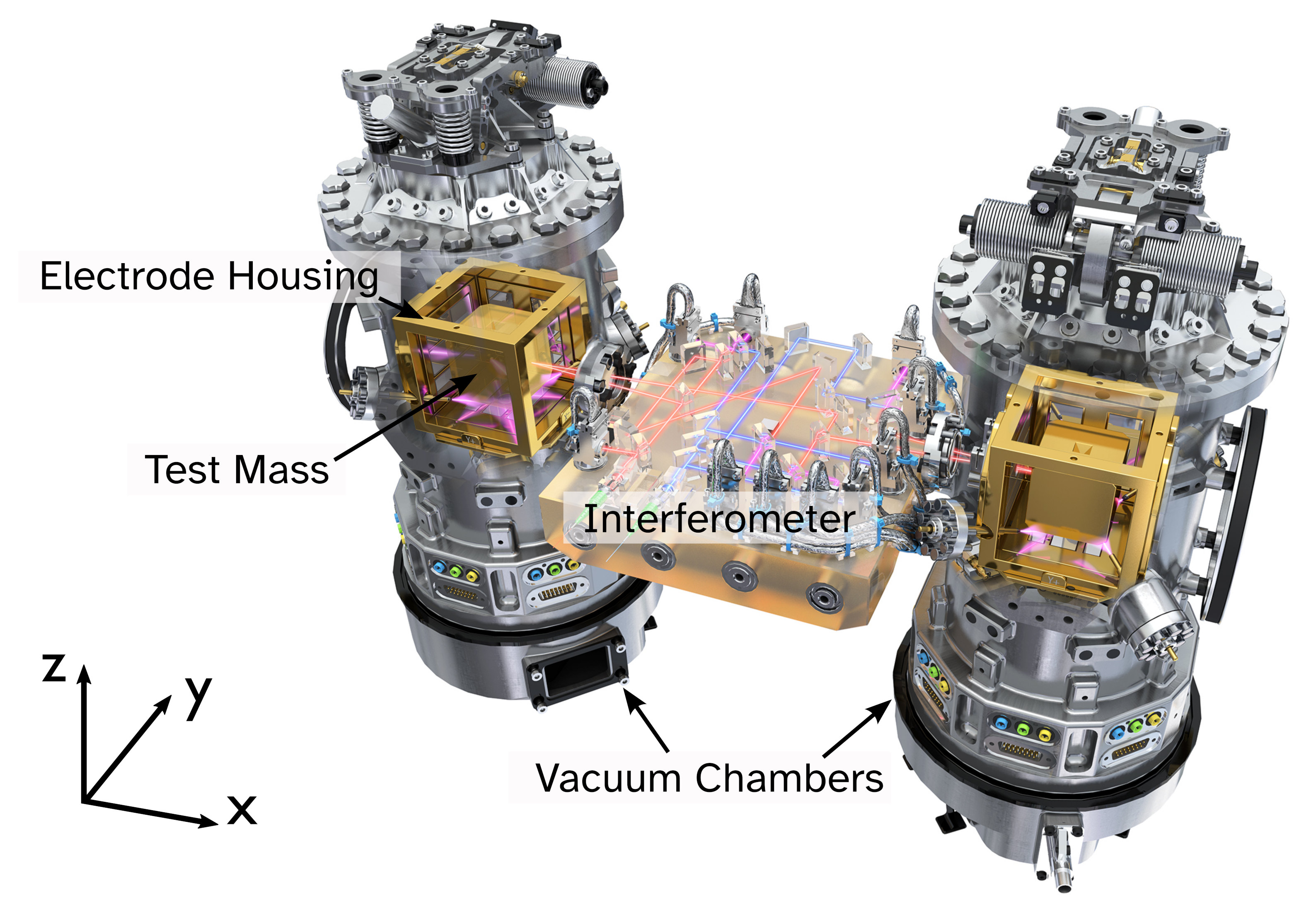
The LTP, depicted in Fig. 1, carried two cubic Au-Pt TMs each with a mass of $M=$1.928\text{\,}\mathrm{k}\mathrm{g}$$ and size $l=$46\text{\,}\mathrm{m}\mathrm{m}$$. During operations, these TMs had no mechanical contact with their surroundings, and were nominally free falling, each one at the center of a housing leaving 3 to $4\text{\,}\mathrm{m}\mathrm{m}$ clearance gaps to the faces of the TM. Each of these electrode housings (EH) carried a series of electrodes facing all faces of the respective TM. These electrodes were used for two purposes. First, they were part of a capacitive sensor of the motion of the TM, relative to its housing, for all degrees of freedom (DOF). Second, they were used to apply electrostatic forces and torques to the TM, whenever needed.

Each EH, with its respective TM, was hosted inside a vacuum chamber, called vacuum enclosure (VE), sealed by a dedicated vacuum valve. The valve connected the VE to a second outer volume that was connected by a vent duct to the outside of the spacecraft.

The VE was needed both to allow for vacuum preparation on ground and to shield the TM from the spacecraft internal outgassing that had been predicted to be too large to achieve the desired vacuum level around a non-shielded TM. Further details about the vacuum preparation and handling are given a bit later.

In what follows we call the Gravitational Reference Sensor (GRS) the system of the TM, its EH and VE, and all related accessories.

The main sensor for the relative motion of the TMs was a heterodyne laser interferometric system, called the Optical Metrology System (OMS) [5]. For the purpose of this paper, it is important to recall that the interferometer measured six different DOF: the relative displacement $\Delta x(t)$ between the TMs along the sensitive $x$-axis, joining their respective centers of mass; the relative displacement $x_{1}(t)$, along the $x$-axis, of one of the TM, called TM1, relative to the interferometer optical bench and, as a consequence, also relative to the spacecraft; the two angles of rotation $\eta(t)$ and $\phi(t)$ for both TMs, around the $y$-axis and $z$-axis respectively. These six TM DOF, and also the remaining six, were also measured at all times by the capacitive sensors [6]. However, the interferometric readout was approximately three orders of magnitude more sensitive than the capacitive one for all DOF for which they were both available. All the data series analyzed in this paper have a sampling rate of $10\text{\,}\mathrm{Hz}$.

Besides the measurement of the TM motion, other physical quantities have been measured, by dedicated instruments, throughout the mission. In particular, we measured: the magnetic field vector at various locations, via a dedicated set of magnetometers [7]; the temperature at various critical locations, via a dedicated set of thermistors [8]; the cosmic ray flux with a radiation monitor [9, 10].

Before closing this section, we want to specify some details of the vacuum handling that are useful for some of the discussions in the following sections.

Once the VE was evacuated on ground, the vacuum valve was closed and the VE remained sealed for a few months, until the valve was opened again once in orbit. Valve opening took place, within an hour for both VE, on February 3, 2016, i.e. $62.4\text{\,}\mathrm{d}$ after the launch. In the rest of the paper, we call $t_{v}$ this time of valve opening, while we call $t_{0}$ the time of the launch, December 3, 2015 04:04:00 UTC. The outer volume, with its vent duct, was not evacuated on ground, and, having no seal, was exposed to space immediately after $t_{0}$.

Besides the TM and EH, the VE contained various metal structural elements, two piezoelectric motors, used to center the TM within the EH and release it into free fall, and various thermistors and heaters. The VE also contained the $\sim 40$ cables needed for all these appliances, which crossed the VE wall through a set of vacuum feed-throughs. Finally, also included in the VE was a $\sim$2\text{\,}\mathrm{k}\mathrm{g}$$ Tungsten balance mass used to suppress the gravitational field at TM location [11]. The outer chamber contained a high-output paraffin motor [12] used to activate the vacuum valve and the TM launch lock, with all the necessary cables.

II.2 Dynamical controls and data series formation

LPF was a controlled dynamical system consisting of the spacecraft and the two TMs. More specifically, the spacecraft was forced to follow one of the TMs (TM1) along $x$ via an active control loop, using the spacecraft cold gas micro-thrusters as actuators [13], known as drag-free control.

Each TM rotation along $\phi$ and $\eta$ was kept fixed relative to the spacecraft by an active loop using electrostatic torques. These torques were applied via the above-mentioned electrodes.

No electrostatic actuation force was applied along $x$ on TM1, while a control loop (electrostatic suspension) kept the distance between the two TMs nominally fixed, by applying a suitable electrostatic force along $x$ on the other TM (TM2). All other degrees of freedom were also controlled, but the details are not relevant here.

As the distance between the TMs was actively controlled, the external, out-of-the-loop, differential disturbance force per unit mass acting on the TMs, $\Delta g_{\text{ext}}$, could not be identified with the in-loop relative acceleration measurement $\Delta\ddot{x}$ [2]. On the contrary, $\Delta\ddot{x}$, which was estimated numerically [14], had to be corrected for the known applied feedback forces per unit mass $g_{c}(t)$ [2].

In addition, acceleration data series were also corrected for the following effects.

• Measured inertial forces per unit mass due to spacecraft rotation $g_{i}(t)$, which include the centrifugal and the Euler force [1]. These effects will not be relevant for LISA [15].

• The forces per unit mass generated by the motion of the TMs through static force gradients in the spacecraft, as LISA data can also be corrected for those. Such force acting on TM$i$ is well approximated by the linear model $-\omega_{i}^{2}x_{i}$, as described in [1].

• The interferometer spurious pick up $g_{\text{CT}}(t)$ of spacecraft motion along DOF different from $x$, due to cross-talk [16, 17]. This also includes the pick-up of the common mode motion of the TMs, described by a term $\delta_{x_{1}}\ddot{x}_{1}$. Some of these effects will also be present in LISA, and will be analogously corrected [15].

Thus the out-of-the-loop, differential force per unit mass data series used in the following analyses, can be written as:

$$\begin{split}\Delta g(t)=&\Delta\ddot{x}_{\text{OMS}}(t)+\omega_{2}^{2}\Delta x_{\text{OMS}}(t)+(\omega_{2}^{2}-\omega_{1}^{2})x_{1,\text{OMS}}(t)\\ &-g_{c}(t)-g_{i}(t)-g_{\text{CT}}(t).\end{split}$$ (1)

Note that, in Eq. (1), we have attached the suffix OMS to all coordinates, to indicate that these have been measured by the relevant interferometers, and not by the capacitive sensors. For these we will use the GRS suffix. Note also that $\omega_{1}^{2}$ and $\omega_{2}^{2}$ above, as well as $\delta_{x_{1}}$, have been measured in dedicated calibration experiments [18]. In particular $\omega_{2}^{2}\approx$-4.5\text{\times}{10}^{-7}\text{\,}\mathrm{s}^{-2}$$ is negative, while the differential stiffness $(\omega_{2}^{2}-\omega_{1}^{2})$ is roughly 20 times smaller and thus neglected in this discussion here.

The feedback force $g_{c}(t)$ in Eq. (1), is the time series of the force that the onboard computer has commanded to the electrostatic force system. It was calibrated through an extensive series of experiments [18], consisting of the application to the TMs of a series of forces oscillating at frequencies $\gtrsim$1\text{\,}\mathrm{m}\mathrm{H}\mathrm{z}$$, and of the measurement of the resulting acceleration, a quantity which is intrinsically calibrated in terms of the laser wavelength and of the onboard clock calibration.

This calibration campaign led us to discover a systematic, non-linear, error in the electronics, originating from an overlooked truncation of the digital voltage commands [19], that resulted in an amplitude-dependent fluctuation of the calibration. Therefore $g_{c}$ had to be recalculated considering such an extra truncation. After this crucial correction, the calibration of $g_{c}$ was found to be stable at better than $<1\%$, independently of the amplitude of the applied forces and torques, throughout the entire mission [18].

$\Delta g(t)$ in Eq. (1) is our best estimate for the external differential force per unit mass $\Delta g_{\text{ext}}$. However the series is corrupted by the noise $n_{\text{OMS}}(t)$ in the differential interferometer readout $\Delta x_{\text{OMS}}$. Such disturbance enters into $\Delta g(t)$ in Eq. (1), both through $\Delta\ddot{x}_{\text{OMS}}(t)$, and through $\omega_{2}^{2}\Delta x_{\text{OMS}}(t)$. Thus, the residual noise in $\Delta g$ can be evaluated as:

$$\Delta g=\Delta g_{\text{ext}}(t)+\ddot{n}_{\text{OMS}}(t)+\omega_{2}^{2}n_{\text{OMS}}(t).$$ (2)

Finally, it is important to mention that occasional force transients were observed in the data [20]. In ordinary runs these glitches occurred at an average rate of $\simeq 1\,\text{d}^{-1}$. These glitches have been removed from the data, as described in Ref. [20], before any noise analysis.

II.3 Data runs

The mission scientific operations lasted from March 1, 2016 to July 18, 2017. During these more than 16 months, we performed many uninterrupted noise runs during which the TMs and the satellite were in steady control conditions, with no purposely applied stimulus of any nature.

We have performed many such noise runs, however we restrict the main analysis to those with an overall duration of at least 2.5 days. Such a duration allows an estimate of acceleration power spectral density (PSD), down to about $\simeq$18\text{\,}\mathrm{\SIUnitSymbolMicro Hz}$$ with reasonable accuracy (see following sections).

We list in Table 1, for all these runs, the start and stop dates, the duration, and the instrument operating temperatures. Temperature values are the average of the 8 thermometers placed on the two GRS as described in [8]. We note that 11 of these runs were performed at an operating temperature around 21-22 $\mathrm{\SIUnitSymbolCelsius}$, while run 10 and 11 were operated at around 11 $\mathrm{\SIUnitSymbolCelsius}$.

TABLE 1: List of the considered noise runs. Run 10 is the February 2017 run published in [1].

N.	Start date	Duration	Mean time	Temperature
		[d]	from launch [d]	[K]
1	2016-03-21	5.3	112	$295.37\pm 0.04$
2	2016-04-04	9.3	127	$295.30\pm 0.03$
3	2016-05-16	3.2	166	$294.97\pm 0.06$
4	2016-06-19	4.8	202	$294.93\pm 0.01$
5	2016-07-17	2.8	229	$296.62\pm 0.05$
6	2016-07-24	5.3	237	$296.50\pm 0.02$
7	2016-09-28	2.8	302	$296.50\pm 0.02$
8	2016-11-16	9.9	354	$296.86\pm 0.04$
9	2016-12-26	18.5	398	$295.38\pm 0.04$
10	2017-02-14	13.3	446	$284.72\pm 0.03$
11	2017-05-18	4.3	535	$284.2\;\pm 0.1$
12	2017-05-29	6.8	547	$295.78\pm 0.01$
13	2017-06-08	8.6	558	$295.91\pm 0.03$

The detailed operating conditions have been slightly different for different runs. We have listed in Table 2, in App. A, the few differences of settings that may bear some relevance for the noise performance.

For runs 1 to 11, the total charge of both TMs was maintained within the interval of $\pm\,3\times 10^{7}\,e$ [21], in order to keep the noise caused by voltage fluctuations negligible [22] (see Sec. VIII.4). For those runs, charge was measured just before and just after each run. For runs 12 and 13, the charge was measured just once before run 12. We could however extrapolate the missing final values from the measurement of cosmic ray flux [21, 23]. For run 12, such extrapolated final value is still in the aforementioned interval, while for run 13 it might have gone up to $4\times 10^{7}\,e$.

TM neutralization was performed using a non-contacting UV discharging system [24] before the start of each run. As cosmic rays resulted in a steady increase of the charge, for most of the runs the charge was brought to a negative value within the $\pm\,3\times 10^{7}\,e$ interval at the start of the run, to have it drifting through zero during the run.

Two major events must be mentioned. First ESA operated LPF, until April 6, 2017, on a Lissajous orbit near the L1 point of the Earth-Sun system. This orbit was unstable, and mission control had to make station-keeping maneuvers every few weeks to maintain it. On April 6, 2017 in preparation for the end of the mission, mission control performed a final maneuver, called “de-orbiting burn”, to place the spacecraft on a trajectory that would not risk intercepting the Earth. The maneuver lasted a few days, and after that, and until the end of the mission, no further station-keeping maneuver was performed.

In addition, between April 30, 2017, and May 16, 2017, with the purpose of further reducing noise beyond the level reached in February 2017 [1], we tried to operate the instrument near $0\text{\,}\mathrm{\SIUnitSymbolCelsius}$, a value well outside its nominal operating range. The instrument entered into a rather unstable state, with a very high rate of glitches [20], and went back to its ordinary behavior only when the temperature was raised back to a value within its operating range.

During such $0\text{\,}\mathrm{\SIUnitSymbolCelsius}$ cooling, we were able to perform a noise run lasting from 2017-05-03 to 2017-05-09 (for a total of $5.8\text{\,}\mathrm{d}$), not listed in Table 1. In this run, despite the low quality of the data, we were able to perform some noise measurements at frequencies around 1 mHz, which we will mention later in the paper, Sec. IV.

Unfortunately, the temperature of this cold run, has not been measured directly, as the electronics of the GRS thermometers clipped at $\simeq$7\text{\,}\mathrm{\SIUnitSymbolCelsius}$$. However we found that, upon a proper calibration, the average of a group of thermometers just outside the instrument bay was a good proxy of the average of the GRS thermometers, at all temperatures above $\simeq$7\text{\,}\mathrm{\SIUnitSymbolCelsius}$$. This proxy gives, for the cold-run, $T\simeq$1.7\text{\,}\mathrm{\SIUnitSymbolCelsius}$\simeq$274.8\text{\,}\mathrm{K}$$ with an overall uncertainty not larger than $0.5\text{\,}\mathrm{K}$.

III Acceleration PSD

During all noise runs we have estimated the PSD of $\Delta g(t)$, $S_{\Delta g}(f)$ (or, equivalently, its square root, the amplitude spectral density (ASD)), as a function of frequency $f$, by using the periodogram method explained in App. B.2. The method gives a Bayesian estimate for the posterior distribution of $S_{\Delta g}(f_{i})$, over a given set of frequencies ${f_{i}}$. The frequencies within the set have been chosen such that the PSD estimates at different frequencies have minimal statistical correlations (see App. C and [1]). In addition, for practical reasons, we have adjusted the selection such that the fourth frequency is 0.1 mHz, the lower bound of the official LISA band.

The blue points in Fig. 2 illustrate the result of the procedure for run 10 of Table 1, which is the February 2017 run that we published in [1].

FIG. 2: Blue points: ASD of $\Delta g(t)$, $S_{\Delta g}^{1/2}$ for run 10 of Table 1 (February 2017) as a function of frequency $f$. The vertical error bars delimit the 1$\sigma$ interval (see footnote on page 1 for the definition). The horizontal bars indicate the effective width of the spectral window contributing to each of the points. Red points: estimated excess over Brownian noise. Green thin band: uncertainty band for the estimate of the Brownian noise.

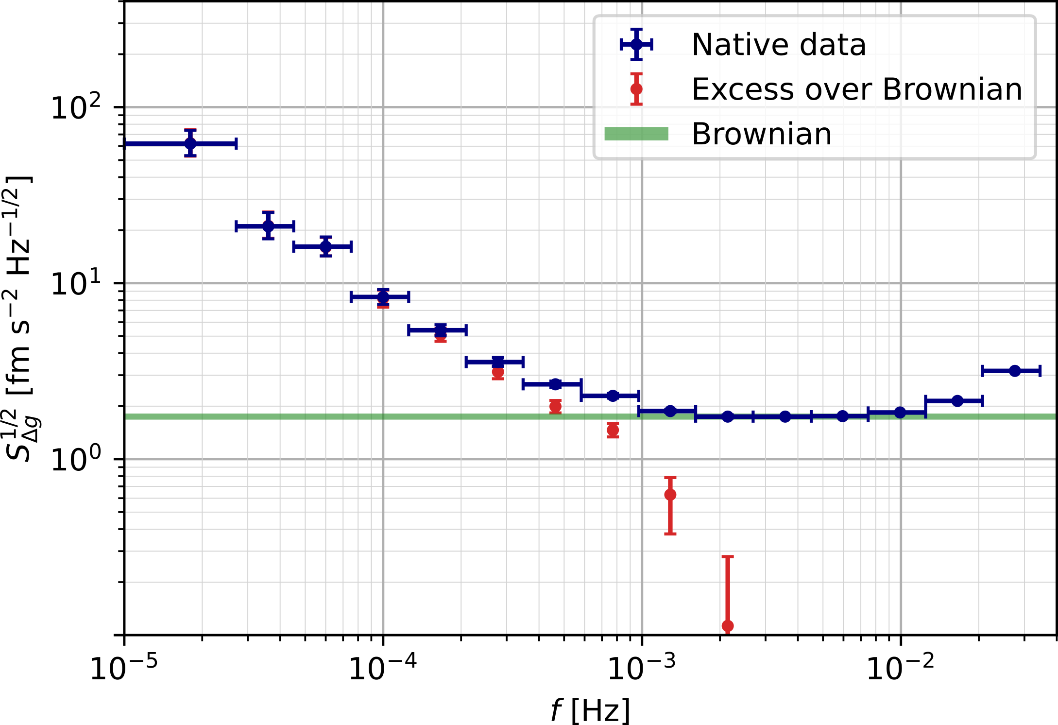
The figure shows that, as already noted in [1], the ASD, and the PSD, have three different branches:

1. a low frequency branch with an approximate $f^{-1}$ behavior ($f^{-2}$ for the PSD);

2. an approximately frequency-independent branch above about 1 mHz;

3. a rising branch above about 10 mHz.

As explained in [2], the rising branch is due to the interferometer readout noise $n_{\text{OMS}}$ and will be not discussed any further.

In [2] we have attributed the frequency independent branch, with PSD value $S_{\text{Brown}}$, to Brownian noise due to gas damping. To separate it from the other two branches, we use, for each run, the following procedure.

FIG. 3: Blue dots: PSD of Brownian noise $S_{\text{Brown}}$ as a function of $(t-t_{v})$, the time since venting of the vacuum enclosure. Error bars correspond to 1$\sigma$ intervals. For convenience, call-outs repeat the mean temperatures $T$ of the runs from Table 1. Blue dot: $S_{\text{Brown}}$ for the cold run ($T\sim$275\text{\,}\mathrm{K}$$). Data may be converted into the mean of the pressures $P_{\text{H}_{2}\text{O}}$ in the two GRS (right vertical scale) by using the conversion factor in [25], and by assuming that the residual gas consists of water molecules. Red dots: PSD of Brownian noise of ordinary runs, scaled as $S_{\text{Scaled}}=S_{\text{Brown}}\,e^{-T_{a}\left(\frac{1}{T}-\frac{1}{T_{0}}\right)}$, with $T_{0}=$293\text{\,}\mathrm{K}$$ and $T_{a}=$7.0\text{\,}\mathrm{kK}$$. Dashed black line: $S_{\text{Scaled}}(t)\propto(t-t_{v})^{-0.80}$. See text for details. Dotted gray line: best fit assuming adsorption quasi-equilibrium. See Sec. VI for details.

• We fit the experimental PSD data $\Pi_{\Delta g,k}(f_{i})$ of run $k$ to the PSD model

  $$S_{\Delta g,k}(f_{i})=S_{\Delta g_{e},k}(f_{i})+S_{\text{Brown},k},$$ (3)

  that is, with a frequency independent term $S_{\text{Brown},k}$, plus the excess $S_{\Delta g_{e},k}(f_{i})$ that depends on the frequency $f_{i}$.

• To avoid numerical instabilities, we limit the analysis to $f<$3\text{\,}\mathrm{m}\mathrm{H}\mathrm{z}$$, that is, to the lowest 10 frequencies of Table 6 in pag. 6. However, to better constrain $S_{\text{Brown},k}$ we add one further data point consisting of the minimum value of $\Pi_{\Delta g,k}(f_{i})$ for $i>10$, $\Pi_{\Delta g,k,\text{min}}$. We fit this data point with the simpler model $S_{\Delta g,k,\text{min}}=S_{\text{Brown},k}$, that is, with no excess over the Brownian noise; this is a reasonable assumption, also supported by the results of the following analyses. This additional term also prevents the fit to put $S_{\text{Brown},k}$ to zero.

• The fit is a Monte Carlo Markov Chain (MCMC) estimate of the posterior

  $$\begin{split}&p\left(S_{\Delta g_{e},k}(f_{i}),S_{\text{Brown},k}|\Pi_{\Delta g,k}(f_{i}),\Pi_{\Delta g,k,\text{min}}\right)_{i\in[1,10]}\propto\\ &\propto\prod_{i=1}^{10}p\left(\Pi_{\Delta g,k}(f_{i})|S_{\Delta g_{e},k}(f_{i})+S_{\text{Brown},k}\right)\times\\ &\times p\left(\Pi_{\Delta g,k,\text{min}}|S_{\text{Brown},k}\right)\end{split}$$ (4)

  Here the function $p(\Pi|S)$, the probability distribution of the experimental PSD, is that given in App. B.2.

• We scan the domain of the logarithm of all parameters $S_{\Delta g_{e},k}(f_{i})$ and $S_{\text{Brown},k}$, and do not multiply the posterior in Eq. (4) by any explicit prior. This is equivalent to using the Jeffreys prior on all parameters [26]. However, again to avoid numerical instabilities, we constrain all PSD parameters, both Brownian and excess, to be larger than $1\,\text{am}^{2}\,\text{s}^{-4}/\text{Hz}$.

The results of such procedure are again shown in Fig. 2 for run 10 of Table 1, and for all runs in Fig. 25 and 26 in App. D.

Note that Fig. 25 and 26 show that the procedure gives consistent results for all runs, with the Brownian uncertainty band always very close to the average of native data in the range $$2\text{\,}\mathrm{mHz}$\leq f\leq$5\text{\,}\mathrm{mHz}$$.

IV Time evolution of Brownian noise

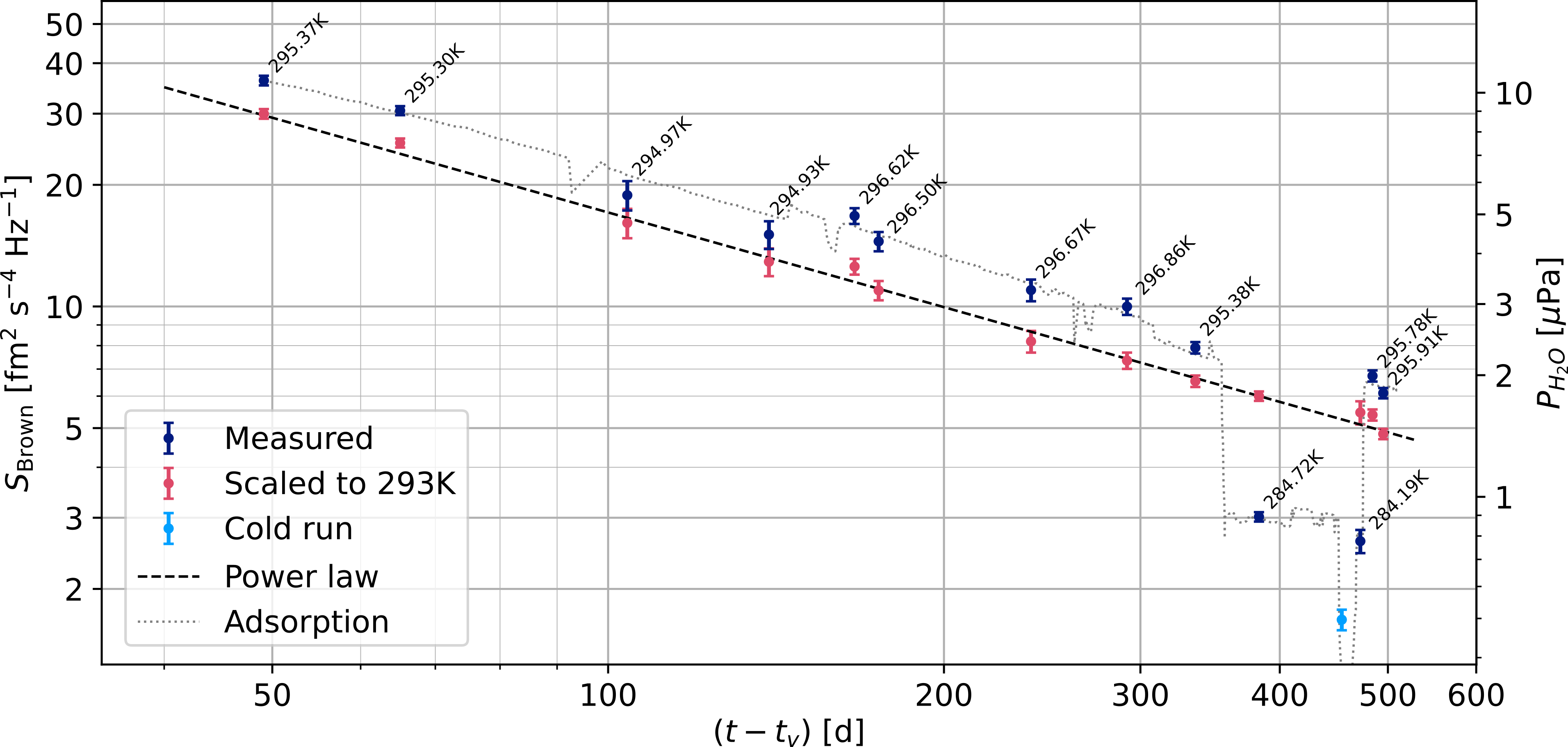
From the procedure described in the previous section, we obtain an estimate of $S_{\text{Brown}}$ for all runs. Results are plotted in Fig. 3, as blue dots, as a function of $t-t_{v}$, the time since venting to space of the VE.

As discussed in [2, 1], the PSD of Brownian noise due to gas damping is expected to be proportional to the gas pressure $P$, with a coefficient of proportionality that depends on the geometry of the TM environment. Ref. [25] estimates such coefficient to be $\kappa\simeq$1.7\text{\,}\mathrm{f}\mathrm{m}^{2}\,\mathrm{s}^{-4}\,\mathrm{Hz}^{-1}\mathrm{/}\mathrm{\SIUnitSymbolMicro}\mathrm{Pa}$$, for a single LPF TM, and for a gas consisting of water molecules. Thus, if indeed the frequency-independent branch represents Brownian noise, $P_{\text{H}_{2}\text{O}}=S_{\text{Brown}}/(2\kappa)$, which can be read on the right vertical axis of Fig. 3, gives a measurement of the mean of the pressures of the two GRS. Note that, with the effective conductance from the interior of the EH to the outer space estimated to be $\simeq$19\text{\,}\mathrm{L}\mathrm{/}\mathrm{s}$$ for water, a pressure of $1\text{\,}\mathrm{\SIUnitSymbolMicro Pa}$ corresponds to an outgassing rate of $1.9\text{\times}{10}^{-7}\text{\,}\mathrm{m}\mathrm{bar}\,\mathrm{L}\mathrm{/}\mathrm{s}$.

The figure also shows that, remarkably, the data can be scaled to follow a straight line, by just multiplying them by a single “activation” factor $e^{-T_{a}\left(\frac{1}{T}-\frac{1}{T_{0}}\right)}$, with $T_{a}$ a properly chosen activation temperature, and $T_{0}$ an arbitrarily chosen, convenient common temperature for the scaled data.

The scaled data may be fit, with comparable qualities, to a few different power-law models, reminiscent of the standard pump-down behavior of vacuum systems [27]. This is discussed in more detail in Sec. VI. The figure reports the result for the case of a VE-dominated outgassing:

$$S_{\text{Brown}}(t)=a\left(\frac{t_{v}}{t-t_{v}}\right)^{\gamma}$$ (5)

where $a$ and $\gamma$ are two fitting parameters. As usual for this kind of pump-down laws, Eq. (5) holds only after the initial rapid pressure decay phase, and should not be extrapolated to $t\to t_{v}$ [28].

Actually a simultaneous fit leaving also $T_{a}$ as a free parameter, gives $T_{a}=(7.0\pm 0.2)\leavevmode\nobreak\ \text{kK}$, $\gamma=(0.80\pm 0.02)$, and finally $a=(27.0\pm 0.7)\leavevmode\nobreak\ $\mathrm{f}\mathrm{m}^{2}\,\mathrm{s}^{-4}\mathrm{/}\mathrm{Hz}$$.

Given the uncertainty on the temperature and on the quality of the PSD data, we have left the cold run datum out of re-scaling and fitting. This is further discussed in Sec. VI. Here we only note that the cold run datum is lower than those for the lowest temperature ordinary runs. This shows that the TM acceleration noise in the mHz bandwidth is truly Brownian down to a level well below $2\text{\,}\mathrm{f}\mathrm{m}\,\mathrm{s}^{-2}\mathrm{/}\sqrt{\text{Hz}}$ per TM, and not saturating to a significant level reflecting other important noise sources in this band.

For the sake of the discussion in Sec. VI, we also report in Fig. 3 the best fit for one common model for vacuum evolution under the hypothesis of quasi-equilibrium between surface water readsorbtion and outgassing. The discussion on Brownian and vacuum environment continues in the mentioned Sec. VI.

V Stability and time evolution of excess noise

In this section we discuss the stability and evolution of $S_{\Delta g_{e}}$, the excess noise over Brownian, over the duration of the mission. The details of the variations of $S_{\Delta g_{e}}$ can be tracked in Fig. 25 and 26 in App. D. Here we present a few summary analyses with the main aim of quantifying noise stationarity.

We first discuss the compatibility of the observations at each frequency with a model considering a single stationary, run-independent, noise process.

Having identified significant variations from run to run of the lowest frequency datum, mostly in the initial phase of the mission, we separate the discussion on the time evolution of the excess noise for $f>$18\text{\,}\mathrm{\SIUnitSymbolMicro Hz}$$ from that at $f=$18\text{\,}\mathrm{\SIUnitSymbolMicro Hz}$$, that we treat in Sec.V.6 together with long-term drifts.

V.1 Fit to a common stationary Gaussian excess for all runs

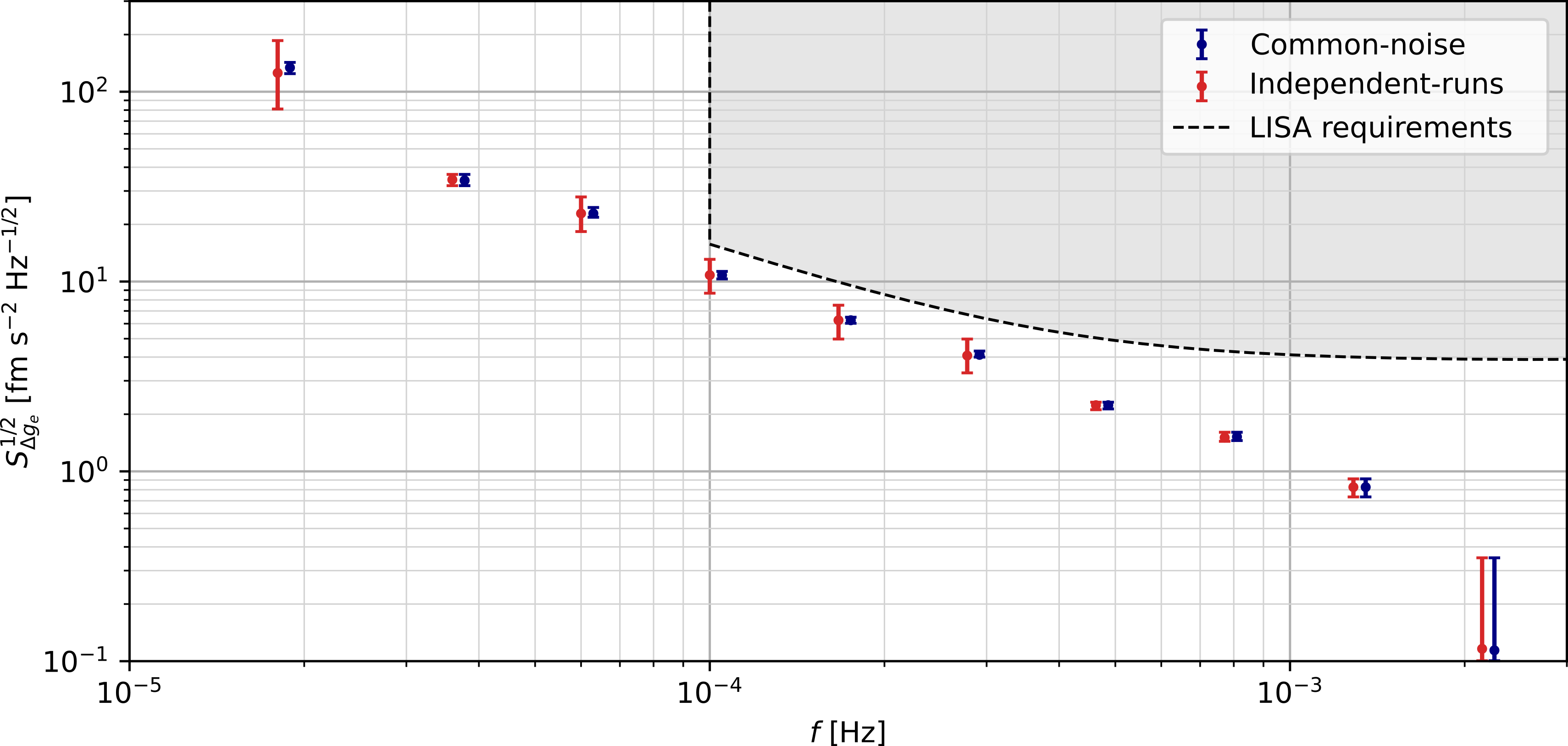
In Fig. 4 we report, at each frequency $f_{i}$, the inferred posterior distribution for $S_{\Delta g_{e}}(f_{i})$ (blue data points) assuming that the excess is a common number to all runs, $S_{\Delta g_{e},k}(f_{i})=S_{\Delta g_{e}}(f_{i})$. We call this the common-noise model. The inference is done by using a collective posterior consisting of the product of the posteriors in Eq. (4), for all values of $k$, having dropped the dependence of the excess on $k$.

FIG. 4: Summary of ASD of $\Delta g$ excess noise, over all runs of Table 1 and Figs. 25 and 26, as a function of the frequency. Blue data: median and $\pm 1\sigma$ quantiles of the inferred posterior distribution of the excess for the entire set of runs, common-noise model (see text for details). Red data: median and $\pm 1\sigma$ quantiles of the inferred posterior distribution, independent-runs model (see text for details). Red data have been slightly shifted in frequency for the sake of readability, but they all refer to the same frequency as that of blue data. Also reported are current LISA requirements adapted from [29].

We have done a simple Akaike information criterion comparison [30] between the common-noise model and the model consisting of the separate Bayesian fits to the data of the 13 different runs discussed in Sec. III. The posterior for the latter is just the product of the posteriors used for the separated fits, and thus depends on 143 parameters: 10 excess noise coefficients for each of the 13 runs, plus 13 Brownian noise coefficients. The common excess noise model depends instead on only 10 excess noise coefficients, and 13 Brownian noise ones, for a total of 23 coefficients.
The Akaike test favors the common-noise model, with a relative likelihood ratio of $\simeq 10^{-20}$. This indicates that the hypothesis of completely independent excess noise values across the runs substantially over-fits the data. However, as usual with Bayesian model comparison, this does not tell if the best of the two fits is a good fit.

We have then done a posterior predictive check [31] on the common-noise model described in the following. We first find the set of parameter values $\hat{\theta}_{\text{best}}=\{S_{\Delta g_{e}}(f_{1}),S_{\Delta g_{e}}(f_{2}),\dots,S_{\text{Brown},1},S_{\text{Brown},2},\dots\}$ that maximizes the posterior likelihood.

Having $\hat{\theta}_{\text{best}}$, for any set of data, either observed or simulated from the posterior, we can then calculate, as a measure of discrepancy at any given frequency $f_{i}$, the log-likelihood of the data at that frequency, conditional on $\hat{\theta}_{\text{best}}$

$$\Lambda_{i}=\sum_{k=1}^{13}\log\,p\left(\Pi_{\Delta g,k}(f_{i})|\hat{\theta}_{\text{best}}\right)$$ (6)

Note that in an ordinary least square fit to independent Gaussian data, the log-likelihood would be, modulo an irrelevant additive constant, just the sum of the square residuals, a quantity commonly used to measure the discrepancy between the data and the model. Thus the use of $\Lambda_{i}$ may be seen as just an extension of the method of square residuals to Wishart-distributed data.

We have then generated simulated data, by sampling the posterior for the parameters $\{S_{\Delta g_{e}}(f_{2}),S_{\Delta g_{e}}(f_{3}),\dots,S_{\text{Brown},1},S_{\text{Brown},2},\dots\}$, and by generating then simulated periodograms $\Pi_{\Delta g,k}(f_{i})$ from the proper Wishart distribution. For each simulated periodogram, we have calculated $\Lambda_{i}$, with $1\leq i\leq 9$ obtaining then an expected posterior predictive distribution for each of these parameters.

We have restricted the analysis to frequencies $f_{i}\leq f_{9}$, as, at higher frequencies, the model breaks down anyway due to the dominance of Brownian noise, particularly for the earlier runs.

We have then calculated the probability $p$ that $\Lambda_{i}$ is less than value $\Lambda_{i,0}$ calculated for the real data, that is the cumulative distribution function for $\Lambda_{i}$ evaluated in $\Lambda_{0,i}$. For $i\in\{2,7,8,9\}$ we find that $p>0.2$, while for the other frequencies we find $p\leq 0.002$. This shows that the common-noise model, despite being more informative than the separated fits, is not predictive of the observations.

To make it predictive, the common-noise model posterior must be widened by a (frequency-dependent) factor. To estimate how large this factor should be, we have repeated the simulation above, this time by generating the simulated periodogram for run $k$ at frequency $f_{i}$, by multiplying the sample for $S_{\Delta g_{e}}^{1/2}(f_{i})$ from the original posterior, common to all runs, by a random variable $\gamma_{k,i}$. For each frequency $f_{i}$, all $\gamma_{k,i}$, were extracted from the same gamma distribution with unit mean value and standard deviation $\sigma_{\gamma_{i}}$. This model in essence allows $S_{\Delta g_{e}}^{1/2}(f_{i})$ to fluctuate from run to run by a mean relative amount $\sigma_{\gamma_{i}}$. This fluctuation adds up to the natural fluctuation of the periodogram for stationary Gaussian time series, in generating the observed data. We call this model the independent-runs model.

The independent-runs model becomes predictive of the observation at all frequencies, $p\geq 0.2$, if $\sigma_{\gamma_{i}}=0$ for $i\in\{2,7,8,9,10\}$, $\sigma_{\gamma_{i}}=0.4$ for $i=1$, and $\sigma_{\gamma_{i}}=0.2$ for $i\in\{3,4,5,6\}$. We report the data for the independent-runs posterior, in Fig. 4, red points.

Note that the largest variation is for $i=1$, that is $f=$18\text{\,}\mathrm{\SIUnitSymbolMicro Hz}$$. This is dominated by the large initial decrease of the ASD in the initial part of the mission that can be noticed by inspection in Fig. 25 on page 25. We will discuss this further in Sec. V.6.

The common-noise model is more predictive for subsets of data including a reduced number of runs. We find for instance that for the groups including runs 1 to 4 of Table 1, and for that including run 11 to 13, the model is reasonably predictive at all frequencies, while for the groups 5 to 8 and 9 to 10, the model is predictive at all frequencies but one. It must be said that other groups of runs, with no temporal continuity, may give similar results, and that this apparent improvement might just be a consequence of the reduced discrimination power of the posterior test if applied to a smaller number of data.

V.2 $1/f$ model, and evolution of the excess noise for $f>$18\text{\,}\mathrm{\SIUnitSymbolMicro Hz}$$

To study if the observed variations of excess noise level are correlated with operational conditions we have found a useful ‘figure of merit’ that summarizes the excess noise across the entire band $f>f_{1}$. We introduce it in the following.

We take advantage of the fact that, as said, the PSD in this frequency band scales approximately as $1/f^{2}$. Thus the coefficient $\widetilde{S}_{\Delta g}$ of the $1/f^{2}$ term in a fit with the model

$$S_{\Delta g}(f_{i})=\widetilde{S}_{\Delta g}\left(\frac{$1\text{\,}\mathrm{mHz}$}{f_{i}}\right)^{2}+S_{\text{Brown}},$$ (7)

gives a reasonable measure of the average power, smoothing any frequency-to-frequency variation. Consistently with the discussion so far, we will focus on the evolution of its square root $\widetilde{S}_{\Delta g}^{1/2}$ and will call this the ‘$1/f$’ model.

To make the analysis consistent, and avoid mixing any effect of the different duration of the various runs, we have partitioned the data for all runs in non-overlapping stretches, all of the same duration of about 2.75 d. This is the duration of the shortest of the runs (run 5 of Table 1). We have then fitted the PSD data for the 27 resulting partitions, to the model of Eq. (7).

The fit was again a Bayesian MCMC analysis, supported by the posterior predictive test based on the likelihood, in close analogy with that used above to test the common-noise model. The only difference is that we now sum the log-likelihood on all frequencies considered. We find that all fits have $p\geq 0.1$ except for one for which $p=0.02$. Actually for 2/3 of the 27 short runs $p>0.5$. The results for $\widetilde{S}_{\Delta g}^{1/2}$ are shown in Fig. 5.

FIG. 5: Time evolution of the $1/f$ tail amplitude of $S_{\Delta g}^{1/2}$, expressed as the corresponding ASD at 1 mHz $\widetilde{S}_{\Delta g_{e}}^{1/2}$, as a function of time since launch $(t-t_{0})$, over the entire mission duration. Blue data: values for all the 2.75 d long, non-overlapping stretches of data into which we partition the full set of the 13 run data series. The gray vertical bands with dashed edges represent the time span of the original runs to which the partition belongs. The picture also shows the date of the initial venting (red line), that of the beginning of the science operations (blue line), the epoch of the de-orbiting burn (green band), and the date of the end of the science operations (magenta line). In cyan the epochs during which the temperature was held at about $11\text{\,}\mathrm{\SIUnitSymbolCelsius}$; runs 10 and 11 of Table 1 are both included in this span. Finally, in blue the epoch of the $0\text{\,}\mathrm{\SIUnitSymbolCelsius}$ cooling.

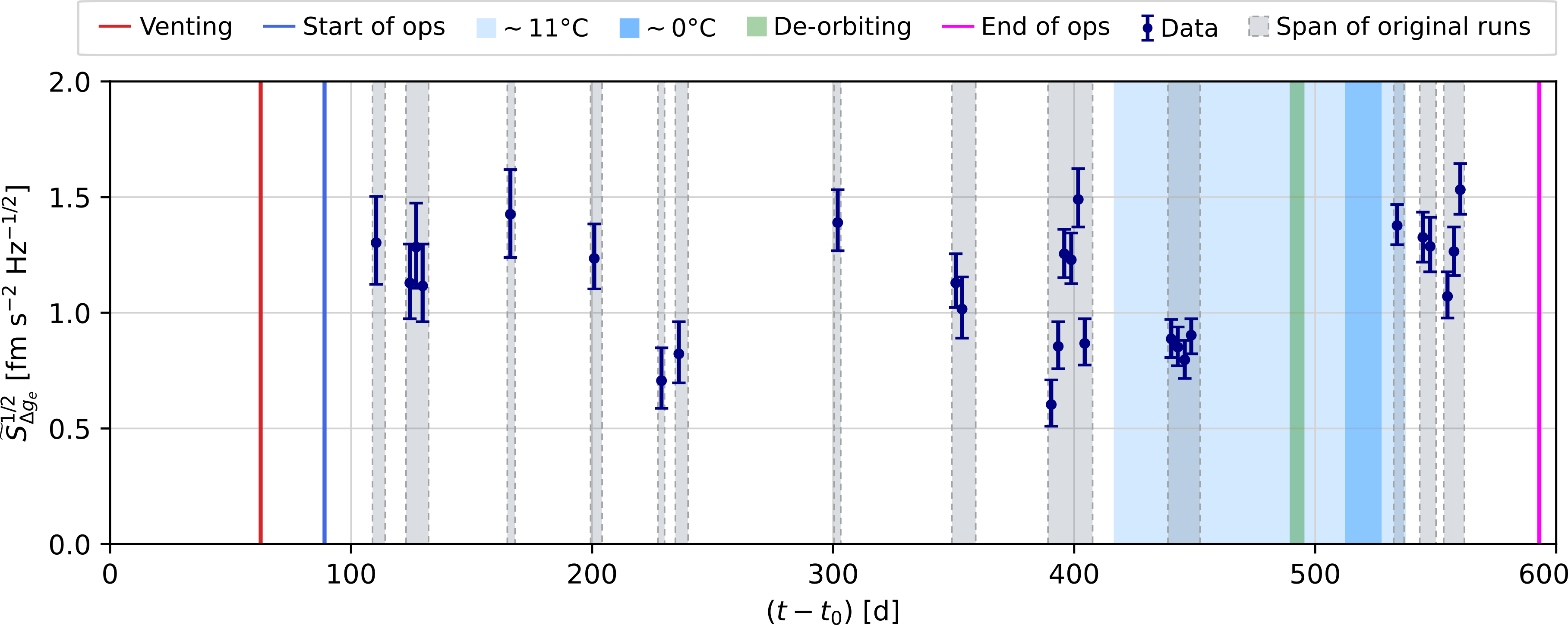
Notice that the LISA requirements for the ASD of $\Delta g$ in Fig. 4, include a $\propto 1/f$ branch, though just down to the lower corner at 0.1 mHz. This branch would correspond to $\widetilde{S}_{\Delta g_{e}}^{1/2}=$1.7\text{\,}\mathrm{f}\mathrm{m}\,\mathrm{s}^{-2}\mathrm{/}\sqrt{\text{Hz}}$$, significantly above all the points in Fig. 5. This is consistent with Fig. 4.

One feature that stands out in Fig. 5 is that data fluctuate significantly more than the uncertainty on the single datum, even for the partitions of the same original run. Actually, the fluctuation of data from partition of run 9, span a similar range than that of the remaining data. This large run-to-run fluctuation appears consistent with the poor fitting to the common-noise model.

Just to confirm that these two facts are consistent, we have simulated the data assuming a common value for $\widetilde{S}_{\Delta g_{e}}^{1/2}$ for all 27 partitions, and Gaussian, stationary noise. This common value is extracted from the posterior for $\widetilde{S}_{\Delta g_{e}}^{1/2}$ of a cumulative fit to all 27 partitions, with a common $1/f$ noise. The model is found, as expected, as non-predictive as the common-noise model for the general case.

To get a useful quantitative statistics to compare the simulated data to the actual ones, we form the sample of the 27 maximum likelihood values for $\widetilde{S}_{\Delta g_{e}}^{1/2}$, in essence, for the real sample, the dots of Fig. 5, and then calculate the sample standard deviation divided by the sample mean $\rho\equiv\sigma_{\tilde{S}_{\Delta g_{e}}}/\langle{\widetilde{S}_{\Delta g_{e}}}\rangle$. For the sample of the actual data, we find $\rho\simeq 0.23$.

The simulation gives instead a mean value for $\rho$ of $\langle\rho\rangle\simeq 0.11$ and projects a probability $<10^{-3}$ of observing a value as large as $\rho=0.23$.

Coherently with findings for the common-noise model, to give such a large value some reasonable probability, we had to widen the posterior, allowing for a 0.2 relative fluctuation of $\widetilde{S}_{\Delta g_{e}}^{1/2}$ from partition to partition.

This is consistent with the observation that, joining the posterior for all 27 partitions, we get that $\widetilde{S}_{\Delta g_{e}}^{1/2}=(1.1\pm 0.3)\,$\mathrm{f}\mathrm{m}\,\mathrm{s}^{-2}\mathrm{/}\sqrt{\text{Hz}}$$, while the width of the posterior for each run fluctuates of about $\simeq 0.1\,$\mathrm{f}\mathrm{m}\,\mathrm{s}^{-2}\mathrm{/}\sqrt{\text{Hz}}$$, implying a true fluctuation of about $\simeq 0.25\,$\mathrm{f}\mathrm{m}\,\mathrm{s}^{-2}\mathrm{/}\sqrt{\text{Hz}}$$ from partition to partition, beyond the statistical uncertainty.

While the data of Fig. 5 do not display any clear systematic long term trend, or correlation with the experimental configuration parameters of Table 2, they show a comparatively large difference, $\simeq 0.45\,$\mathrm{f}\mathrm{m}\,\mathrm{s}^{-2}\mathrm{/}\sqrt{\text{Hz}}$$, between the mean value of the 4 partitions of run 10 (438-451 days after launch in Fig. 5), and that of the six last partitions of runs 11 to 13 (531-561 days after launch in Fig. 5).

Actually the difference is not much less, $\simeq 0.32\,$\mathrm{f}\mathrm{m}\,\mathrm{s}^{-2}\mathrm{/}\sqrt{\text{Hz}}$$, if, instead of just taking the mean of the partitions of run 10, one also adds the 6 partitions belonging to run 9, as run 9 and 10 could be reasonably fit together with the common-noise model, as could also runs 11 to 13. The observation is particularly intriguing, as the $0\text{\,}\mathrm{\SIUnitSymbolCelsius}$ cooling, with its rather dramatic consequences [20], and the de-orbiting burn took place just between these two epochs.

In the attempt to assess if the observed variation could still be due to a random fluctuation, given the comparatively large spread of the values in Fig. 5, we have resorted to a classical permutation test. We have done random permutations of the time coordinates of the data of Fig. 5, and counted the number of times a step of any sign, larger than the observed one, could be found between two adjoining sets of data, one 6-sample long, like that of run 11 to 13, and the other either 4- or 10-sample long.

We find that the fraction of permutations in which we find a step $\leq 0.45\,$\mathrm{f}\mathrm{m}\,\mathrm{s}^{-2}\mathrm{/}\sqrt{\text{Hz}}$$, between the 6-sample and the 4-sample sets, is $p=0.09$, while for the 10- and 6-sample case, the chances of a step $\leq 0.32\,$\mathrm{f}\mathrm{m}\,\mathrm{s}^{-2}\mathrm{/}\sqrt{\text{Hz}}$$ is $p=0.12$. These fractions are both too large to allow us to rule out the hypothesis that the observed increase is due to a random fluctuation.

V.3 Gaussianity

Besides the lack of stationarity discussed so far, non-Gaussian distributed data may also contribute to the discrepancy between a simple common-noise model and the data. We have performed a coarse test on the Gaussianity of the periodograms used to calculate all experimental PSDs.

We have first taken the real and the imaginary parts of all periodograms used to produce the PSD at a given frequency and for a given run, and merged them into a single sample. This to increase the statistics for those frequencies and those runs for which the number of averaged periodograms was very small. We have done this merging taking advantage of the fact that for Gaussian data the real and the imaginary part are independent and have the same distribution.

We have then standardized each sample, by subtracting its mean and by dividing by its standard deviation. Limiting the analysis to the lowest 9 frequencies we then have $9\times 13=117$ of these samples, as the number of runs is 13. The number of periodograms in each sample may vary quite significantly, ranging from 2, for the lowest frequency bin and the shortest runs, up to 512 for $f_{9}$ and run 9. We exclude cases with just one periodogram, as the normalization procedure would be not significant.

As all elements of these 117 samples are normalized, if data are Gaussian, they should all come from the same zero-mean, unit variance Gaussian distribution. We have then merged them all in a single sample containing 12684 standardized periodograms. In Fig. 6 we report the histogram of this sample and, for comparison, the probability density function of the zero-mean unit variance Gaussian distribution.

FIG. 6: Green bars: histogram of the periodogram amplitudes standardized as explained in the text. Solid black line: probability density function of the zero-mean unit variance Gaussian distribution.

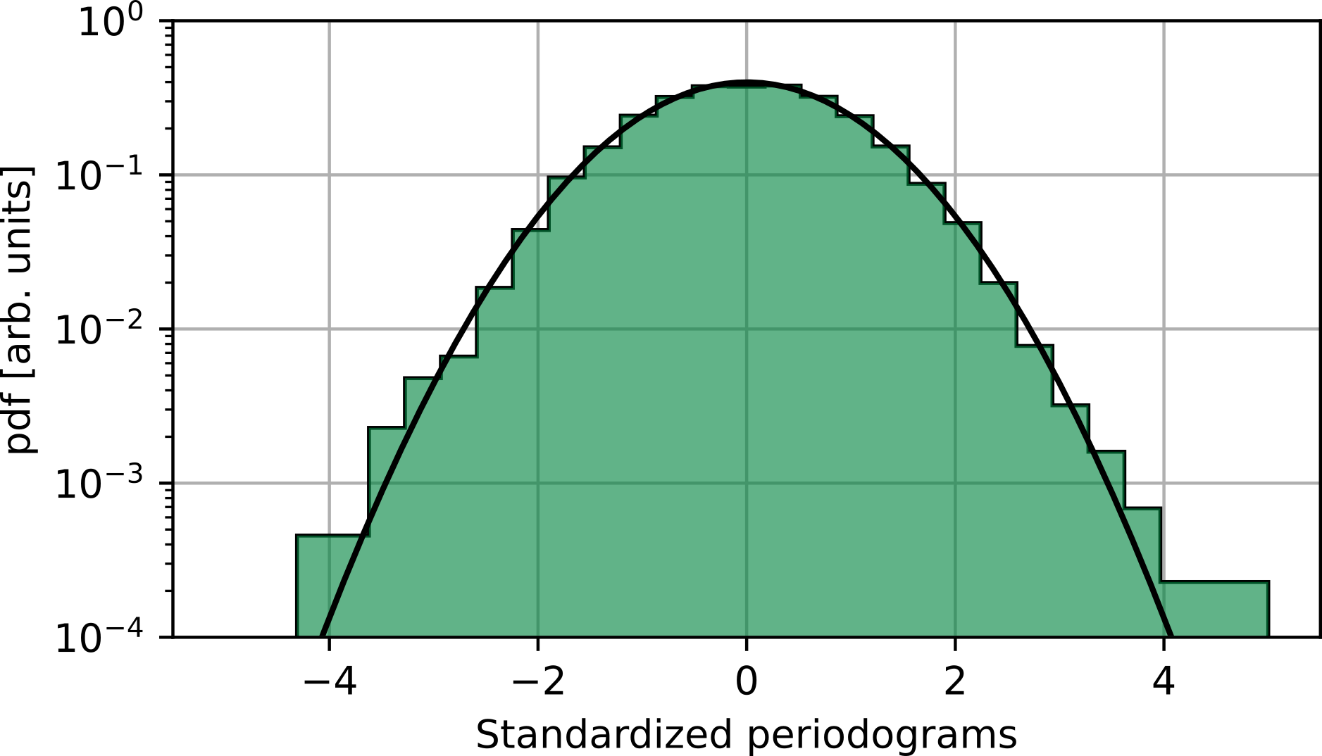
The agreement between the two is supported by an Anderson-Darling test for Gaussianity, that gives $p>0.15$. We note that the test is rather crude, the statistic being dominated by the longest runs and the higher frequencies. However, the absence of any outlier significantly above $5\sigma$ excludes the presence of significant long tails.

V.4 Associated angular acceleration noise

For the purpose of characterizing the properties of the excess acceleration noise described above, we have investigated if there is any torque associated with it. To this purpose, we have measured the torque acting on the test masses around $z$ and $y$.

As the rotation of the test masses around all axes is controlled, and as the angular acceleration of the spacecraft, which is common mode for both TM, is rather large, in total analogy with the $\Delta g$ and the motion along $x$, we form the differential, open-loop torque (per unit moment of inertia) acting on the test mass:

$$\begin{split}&\Delta\gamma_{\phi}=\ddot{\phi}_{2}-\ddot{\phi}_{1}-\frac{N_{z_{2}}-N_{z_{1}}}{I_{zz}}+\omega_{\phi_{2}}^{2}\phi_{2}-\omega_{\phi_{1}}^{2}\phi_{1}\\ &\Delta\gamma_{\eta}=\ddot{\eta}_{2}-\ddot{\eta}_{1}-\frac{N_{y_{2}}-N_{y_{1}}}{I_{yy}}+\omega_{\eta_{2}}^{2}\eta_{2}-\omega_{\eta_{1}}^{2}\eta_{1},\end{split}$$ (8)

Here ${\phi}_{i}$ and ${\eta}_{i}$ are the angular displacements of TM$i$ along $z$ and $y$ respectively, $N_{z_{i}}$, $N_{y_{i}}$ are the control torques applied to TM$i$ along $z$ and $y$ respectively, $I_{zz}$ and $I_{yy}$ are the TM moments of inertia around $z$ and $y$ respectively, and finally the $\omega$’s are the angular stiffnesses. All signals had to be properly calibrated to ensure that the large, common mode angular acceleration of the spacecraft was duly suppressed.

The PSDs $S_{\Delta\gamma_{\phi}}(f)$ and $S_{\Delta\gamma_{\eta}}(f)$ are reported in Fig. 7 for run 10 of Table 1.

FIG. 7: PSD of $\Delta\gamma_{\phi}(f)$ and $\Delta\gamma_{\eta}(f)$, as a function of frequency $f$, for run 10 of Table 1 (February 2017). The green band represents the uncertainty range for the projection of the PSD of the rotational Brownian noise around $\phi$, from the corresponding Brownian noise for $\Delta g$ (see text for details). The reported error on the projected value accounts just for the propagation of statistical errors. Additional inaccuracy due to various sources may amount to some additional 10%.

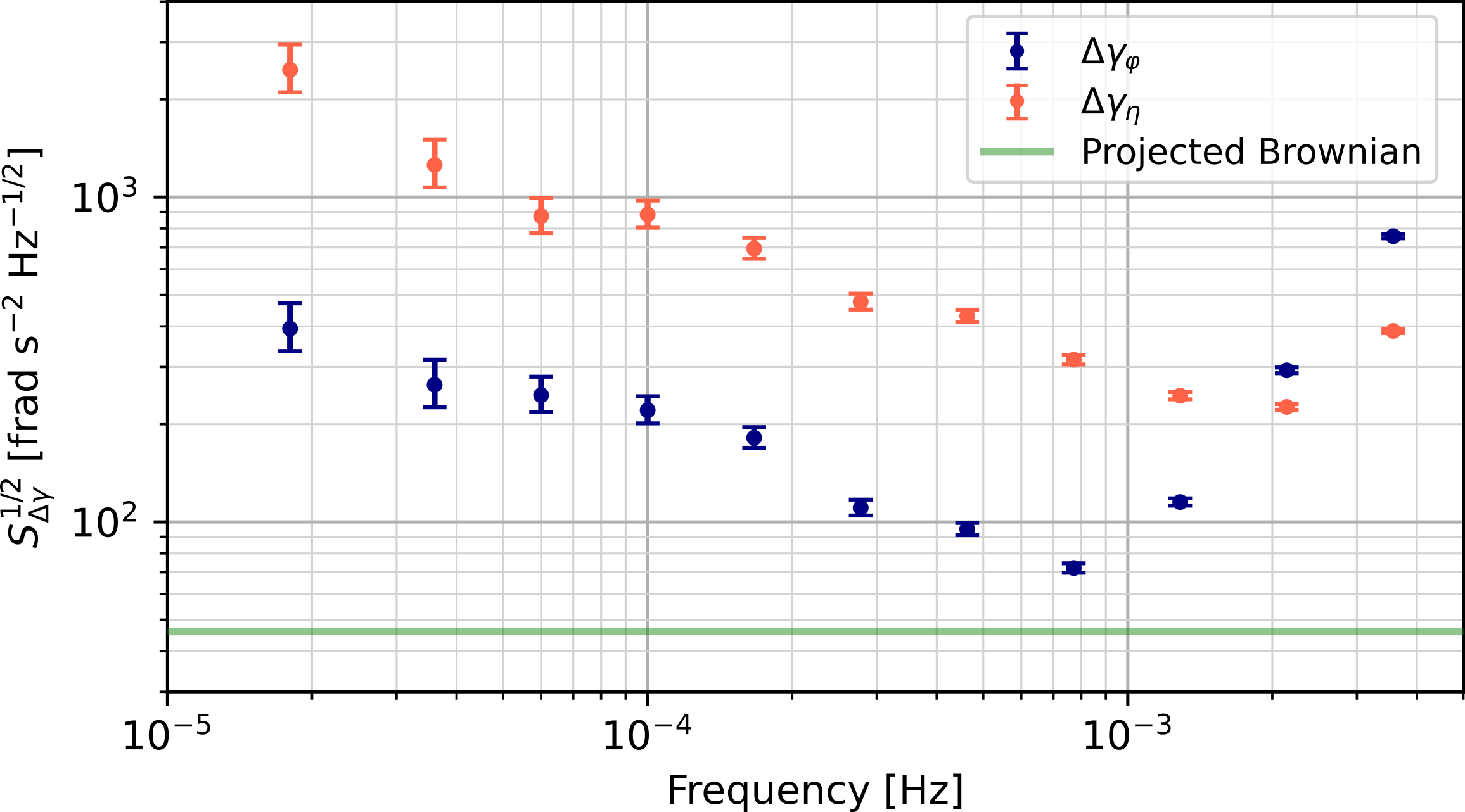
The figure also shows the PSD of rotational Brownian noise along $z$, projected from the measured value of the PSD of the Brownian noise in $\Delta g$ for the same run. The projection is based on calculating the rotational viscous damping coefficient from the linear one, as explained in [25].

Both $S_{\Delta\gamma_{\phi}}(f)$ and $S_{\Delta\gamma_{\eta}}(f)$ show a minimum much larger than the projected Brownian noise. This minimum is set by the cross-over between the torque noise and the readout noise due to the angular interferometer, which is comparatively more noisy than the linear one.

To assess if the excess $\Delta g$ noise carries any torque, we have measured, together with the PSDs, also the cross-spectral densities among $\Delta\gamma_{\phi}$, $\Delta\gamma_{\eta}$, and $\Delta g$.

To get a simple parametrization of the associated torque we use the simple model of a vector point-like force ${f}(t)$, applied to one of the test masses at the point $(x_{0},y_{0},z_{0})$, relative to the test mass center, and with component $(f_{x}(t),f_{y}(t),f_{z}(t))$. Such force would also apply a torque $N(t)$ with $z$ and $y$ components given, respectively, by $N_{z}(t)=x_{0}f_{y}(t)-y_{0}f_{x}(t)$ and $N_{y}(t)=z_{0}f_{x}(t)-x_{0}f_{z}(t)$. For such a force,

$$\begin{cases}&S_{\Delta\gamma_{\phi}}(f)=S_{\Delta\gamma_{\phi},0}(f)+y_{0}^{2}\left(\frac{M}{I_{zz}}\right)^{2}S_{\Delta g}(f)\\ &S_{\Delta\gamma_{\phi}\Delta g}(f)=-y_{0}\left(\frac{M}{I_{zz}}\right)S_{\Delta g}(f)\\ \end{cases}$$ (9)

and similarly for y, with $-y_{0}\rightarrow z_{0}$. Here, $S_{\Delta\gamma_{\phi},0}(f)$ ($S_{\Delta\gamma_{\eta},0}(f)$) is the spectral density of any part of $\Delta\gamma_{\phi}(t)$ ($\Delta\gamma_{\eta}(t)$) that is not correlated to $\Delta g(t)$.

The parametrization holds for an arbitrary system of forces, but while for a real point-like force $\lvert y_{0}\rvert,\lvert z_{0}\rvert\leq l=$46\text{\,}\mathrm{m}\mathrm{m}$$, for an arbitrary system both parameters can take any value. One important example is that of the force due to a voltage on only one of the electrodes facing the $x$-faces of the TM, for which $|y_{0}|\simeq$11\text{\,}\mathrm{m}\mathrm{m}$$ while $z_{0}=0$.

We have estimated the Bayesian posterior for the parameters $S_{\Delta\gamma_{\phi},0}(f)$, $S_{\Delta\gamma_{\eta},0}(f)$, $y_{0}$ and $z_{0}$ with an MCMC calculation, assuming Gaussian data, a Jeffreys prior for $S_{\Delta\gamma_{\phi},0}(f)$, $S_{\Delta\gamma_{\eta},0}(f)$, and a uniform prior for $y_{0}$ and $z_{0}$. We performed this analysis including frequencies from the second to the seventh frequency bins ($36\text{\,}\mathrm{\SIUnitSymbolMicro Hz}$ – $0.60\text{\,}\mathrm{mHz}$), as in some of the runs, some eighth-frequency data already include the interferometer rising branch.

We have performed the calculation for both the individual runs, and also by assuming that the same value of $y_{0}$ or $z_{0}$ may fit all runs. The results are reported in Fig. 8.

FIG. 8: Top panel. Data points: effective lever arm $y_{0}$ of force noise around the $z$-axis as a function of the epoch $t$ of the run. Error bars are $1\sigma$ width of the posterior. Light gray band $y_{0}=(1.13\pm 0.15)\,\text{mm}$, the estimated value of the lever arm assuming a common value for all runs. Bottom panel. Same as the top panel, but for the effective lever arm $z_{0}$ of force noise around the $y$-axis. The light gray band is for $z_{0}=(0.5\pm 0.8)\,\text{mm}$.

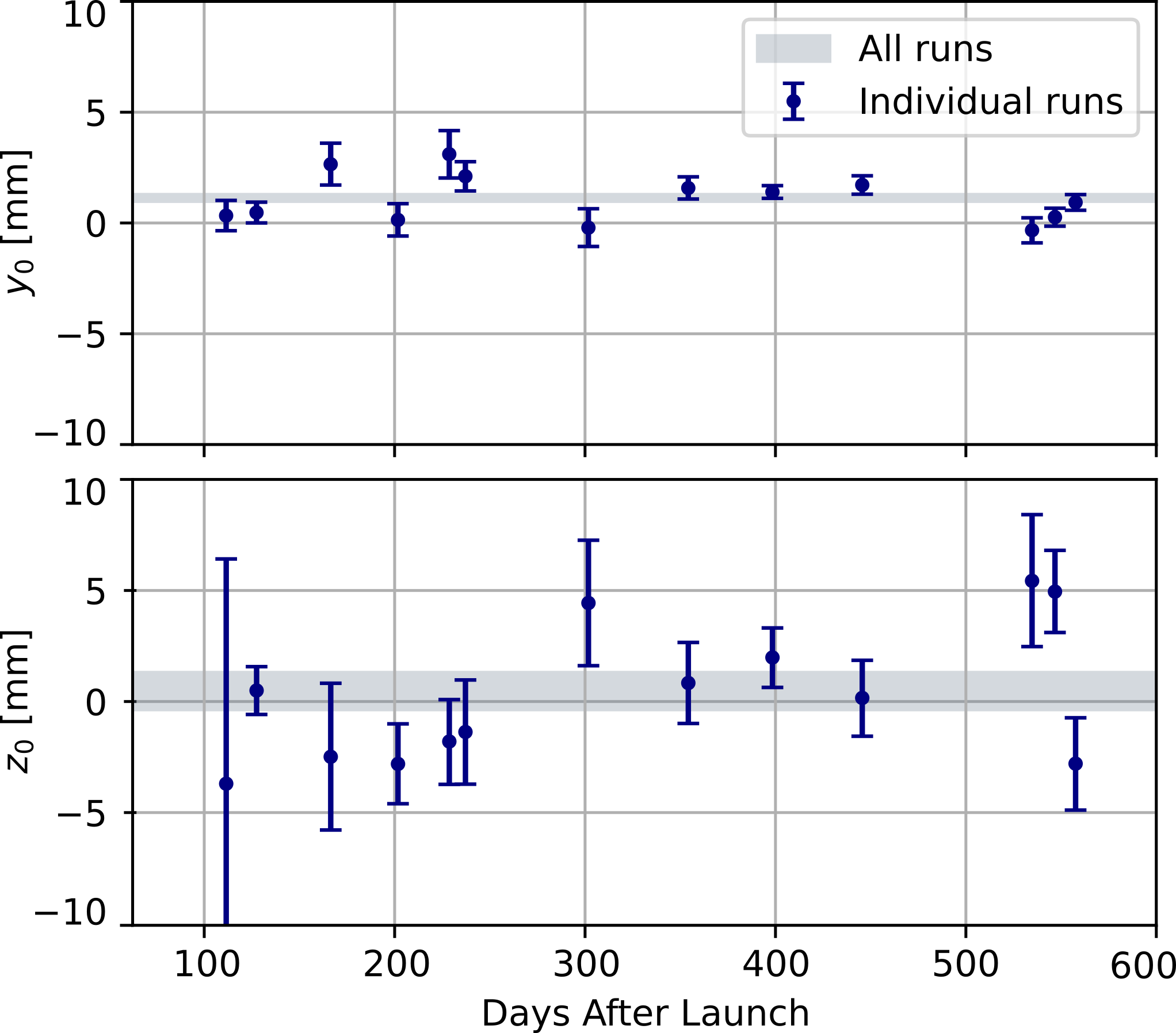
We note that for $y_{0}$ a systematic pattern appears, with the global fit giving $y_{0}=(1.13\pm 0.15)\,\text{mm}$, excluding then $y_{0}=$0\text{\,}\mathrm{m}\mathrm{m}$$ and $y_{0}=$11\text{\,}\mathrm{m}\mathrm{m}$$ with very large significance. On the contrary, for $z_{0}$ data scatter on both sides of zero and the global fit gives $z_{0}=(0.5\pm 0.8)\,\text{mm}$, i.e. a lever arm not significantly different from zero, though within an error which is significantly larger than that for $y_{0}$.

Ref. [32] analyzes the force and torque noise due to gain fluctuations in the LPF TM actuation systems (see also Sec. VIII.4). That study has found that the $\phi$ angular acceleration noise excess at low frequencies is largely explained by actuation gain fluctuations in the circuitry used to produce both $x$ forces and $\phi$ torques. Additionally, that study observes a slight correlation between $\Delta g$ and $\Delta\gamma_{\phi}$ arising from the gain fluctuations in these shared $x$-$\phi$ actuators, a correlation that is consistent with the $y_{0}$ armlength in the top panel of Fig. 8. The slightly positive armlength comes from a slight asymmetry in the electrode voltage noises, as better explained in Ref. [32].

We have compared the results of our analysis, in particular for run 10 of Table 1, to those in [32], and have found full compatibility between them, indicating that the detected torque noise correlated with $\Delta g$, is entirely explained by the shared gain fluctuations. We will further discuss the implications of these findings later in the paper, Sec. IX.

V.5 Summary note on the $1/f$ tail

In conclusion, the overall picture is that, for frequencies in the range [$36\text{\,}\mathrm{\SIUnitSymbolMicro Hz}$ – $0.60\text{\,}\mathrm{mHz}$] the noise ASD for $\Delta g_{e}$ is:

• basically compatible with the $1/f$ model within a single run of $\simeq 2.5\,\text{d}$ duration;

• the ‘true’ amplitude of the $1/f$ branch may fluctuate on the average by $\simeq\pm 20\%$ from one of these runs to another, this fluctuation being in addition to that expected from Gaussian stationary noise;

• the amplitude of such a non-stationary extra fluctuation does not seem to follow any long-term pattern, neither decaying nor increasing over the course of the mission;

• there is no proven correlation between these extra fluctuations and any identifiable operational condition, though we cannot exclude that the $0\text{\,}\mathrm{\SIUnitSymbolCelsius}$ cooling, or the de-orbiting burst may have had some effect on the noise after day 460 (runs 11-13);

• there is a small correlated torque associated with such $1/f$ force noise. The mm-size effective radius points to forces acting toward the center of the TM, or to forces that are almost uniform over the TM faces, ruling out simple possibilities like the force due to a noisy voltage on one of the $x$-electrodes;

• finally, it is worth noting that the approximate stability of the $1/f$ tail’s amplitude persisted despite numerous changes to the operational environment including station keeping maneuvers, planned experiments with the LTP and DRS payloads, and unplanned spacecraft anomalies. By comparison, LISA operations will be simpler with no orbital station keeping or planned experiments post commissioning.

V.6 Evolution of the lowest frequency datum and of long-term drifts

In Sec. V, we noted that the first-frequency point ($f_{1}=$18\text{\,}\mathrm{\SIUnitSymbolMicro Hz}$$) deviates from the $1/f$ ASD behavior, consistently showing a noise level above that predicted by the $1/f$ fit model. To quantify the deviation from the model, we define $\widetilde{S}_{\Delta g_{e}}(f_{1})$, i.e. the excess noise at frequency $f_{1}$, above $\widetilde{S}_{\Delta g}$:

$$\widetilde{S}_{\Delta g_{e}}(f_{1})\equiv(f_{1}/$1\text{\,}\mathrm{mHz}$)^{2}S_{\Delta g_{e}}(f_{1})-\widetilde{S}_{\Delta g}$$ (10)

We have multiplied the data by the frequency factor $(f_{1}/$1\text{\,}\mathrm{mHz}$)^{2}$ to make the comparison with the $1/f$ branch more immediate.

In Fig. 9 (grey points) we show the time evolution of $\widetilde{S}_{\Delta g_{e}}(f_{1})$ at the lowest frequency. Despite the large errors, the picture shows a significant initial decay pattern. In addition, all values of $\widetilde{S}_{\Delta g_{e}}(f_{1})$ are significantly above zero, i.e. there is a noise excess above the $1/f$ model at $18\text{\,}\mathrm{\SIUnitSymbolMicro Hz}$ at all times during the mission.

FIG. 9: Evolution of the excess noise at the lowest frequency $f_{1}=$18\text{\,}\mathrm{\SIUnitSymbolMicro Hz}$$ over the course of the mission. Grey points: $\widetilde{S}_{\Delta g_{e},1}\equiv\left(f_{1}/$1\text{\,}\mathrm{m}\mathrm{H}\mathrm{z}$\right)^{2}S_{\Delta g_{e}}(f_{1})$, for the 13 runs of Table 1, as a function of the mean time of the run since launch $(t-t_{0})$. Red points: residual after correcting for the effect of the temperature, (see text at the end of the section for details). Only data for runs with more than one periodogram at $18\text{\,}\mathrm{\SIUnitSymbolMicro Hz}$ could be corrected, hence in some cases there is no red point (see. App. B.3.2).

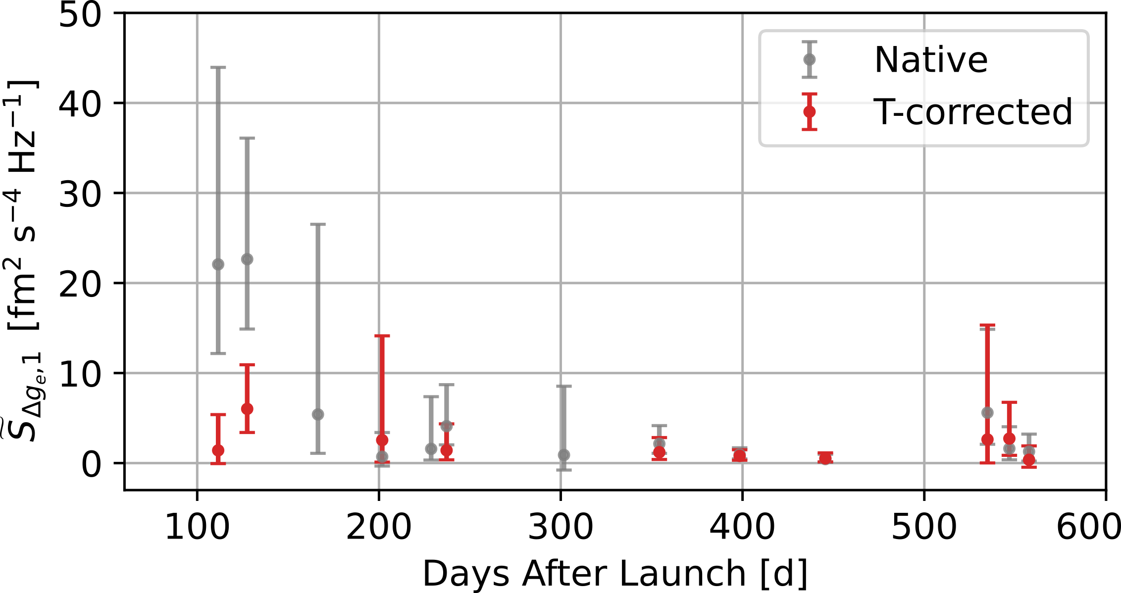
Before discussing this behavior in further detail, and before introducing the temperature correction shown by the red points in the figure, we have to discuss the long-term drift, over scales of several hours and days, that affects $\Delta g$ data for all runs. We will show that such drifts share many of the features shown by $\widetilde{S}_{\Delta g,e}(f_{1})$.

This is not surprising as the relative width of the spectral window at $f_{1}$ is wider, by construction, than that for all other frequencies (See App. B.2). Thus a significant spectral leakage from the frequency band $f\ll f_{1}$, i.e. from the long-term drifts may be naturally expected.

An example of the drift that, in addition to quasi-stationary noise, affects $\Delta g$ data for all runs is shown in Fig. 10.

FIG. 10: Long-term evolution of $\Delta g$ for run 7 of Table 1 (purple line), and of various disturbances that may contribute to it. Green line: gravitational signal from propellant tank depletion. Yellow line: mechanical distortion calculated assuming the nominal value of effective stiffness $\omega_{d}^{2}$. Orange line: temperature contribution from best fit to data. Dashed cyan line: residual drift. See text for details.

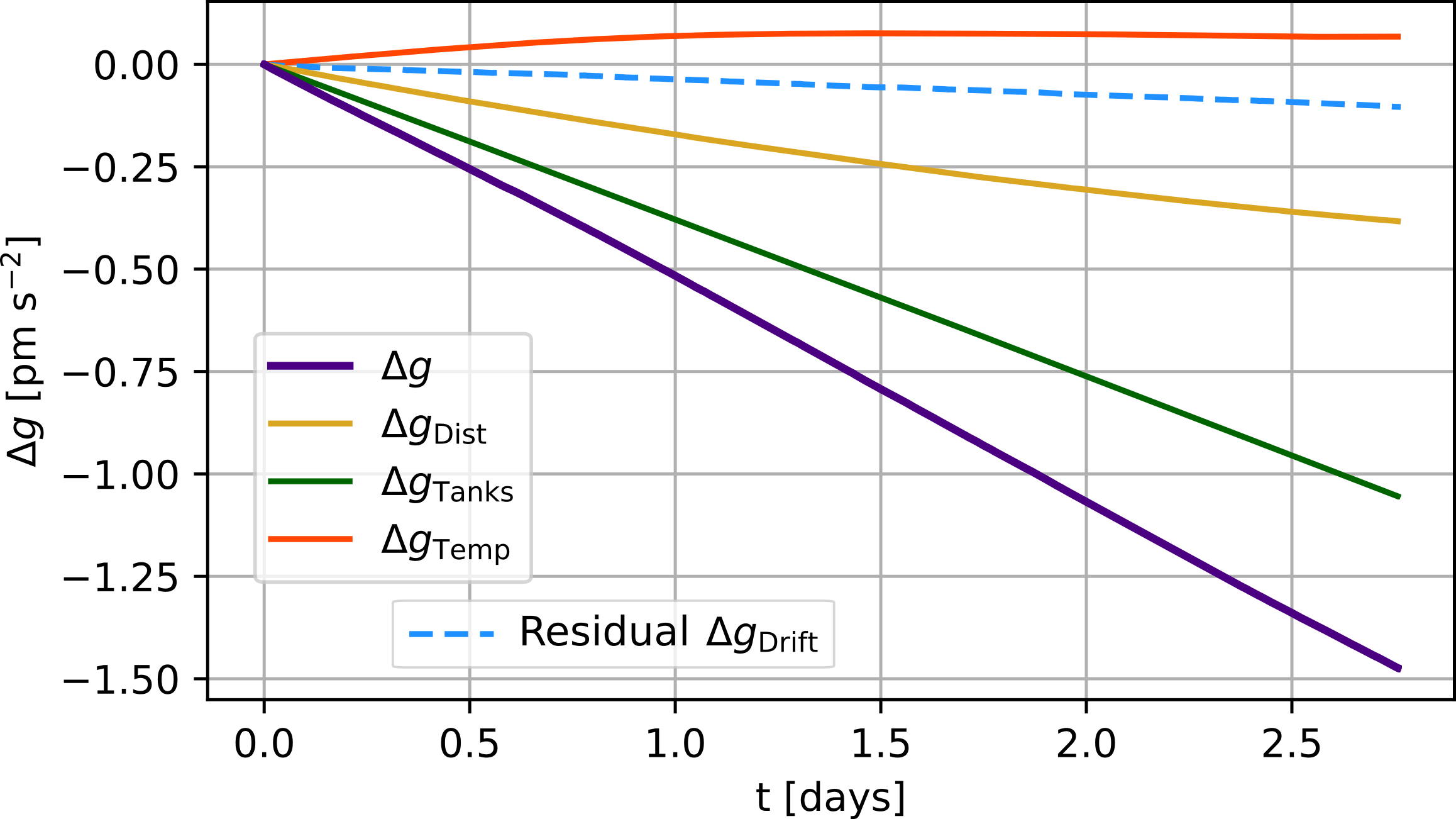
The sources for such a drift may be many. There are two predictable ones:

• motion of massive parts of the instrument relative to the TMs, due to any kind of mechanical distortion, also produces a time-varying gravitational field and then a time-varying $\Delta g_{\text{Dist}}$. One important mechanical distortion is the rigid translation, along $x$, of each GRS relative to its own TM due to expansion and contraction of the optical bench to GRS separation. By GRS we mean here vacuum chamber, electrode housing, etc., but not the TM itself.

  Such distortion is rather likely, as the GRS has a rather complex interface, on one hand to the satellite, via a set of tens of centimeters long ceramics struts, and, on the other, to the optical metrology, through a sophisticated metal-glass interface. This mounting method is rather ‘soft’ and prone to strain, while the GRS itself is a much more rigid assembly.

  Fortunately, the capacitive motion sensor gives a measurement of the relative motion of the GRS relative to its own TM, $\Delta X\equiv\left(\Delta x_{\text{OMS}}-\Delta x_{\text{GRS}}\right)$, and allows to predict $\Delta g_{\text{Dist}}$, as $\Delta g_{\text{Dist}}=\omega_{d}^{2}\Delta X$ (see Fig. 10) with $\omega_{d}^{2}$ a stiffness factor which is known to within a sufficient accuracy. This is again explained in App. E.

  We note that this contribution to the overall drift is rather small, if not negligible, for all runs, except that for runs 7, 11, and 12 of Table 1.

• The use of propellant for the drag-free control slowly depletes the propellant tanks [13]. The propellant in the tanks produces a gravitational field at the TM’s location that results in a differential acceleration of the TMs with a significant component $\Delta g_{\text{Tanks}}$ along $x$. Due to depletion, this acceleration drifts in time (see Fig. 10). In App. E we show that, for a run in which the propellant tank $i$ and the thruster branch $j$ are used, $\Delta g_{\text{Tanks}}(t)=\kappa_{t,i}\kappa_{b,j}\Delta g_{\text{Tank},0,i,j}(t)+c$, where $\Delta g_{\text{Tank},0,i,j}(t)$ is a signal that can be entirely calculated, $\kappa_{t,i}$ and $\kappa_{b,j}$ (where $t$ stands for tanks and $b$ stands for branch) are two factors that reflect calibration uncertainty, and that are both 1 for the nominal case; $c$ is a constant, depending on $i$ and $j$, with no real relevance for the following discussion.

Once the two sources above have been subtracted from the $\Delta g$ data series, the residual shows an evident correlation with the instrument temperature $T$, defined in Sec. II.3, and its long-term variations (Fig. 10). Once also such correlation has been suppressed, by linear least squares fitting $T$ to $\Delta g$ and by subtracting the best fit, still, some residual drift remains (Fig. 10).

We note from Fig. 10 that the raw drift (purple line) is of order $0.5\text{\,}\mathrm{p}\mathrm{m}\,\mathrm{s}^{-2}\mathrm{/}\mathrm{d}$, while the residual unmodelled drift (dashed blue line) is of order $60\text{\,}\mathrm{f}\mathrm{m}\,\mathrm{s}^{-2}\mathrm{/}\mathrm{d}$.

To get some quantitative estimate of this residual drift, we have preliminarily corrected the data for the two predictable effects, $\Delta g_{\text{Tanks}}$ and $\Delta g_{\text{Dist}}$, and then fitted the corrected data to a linear combination of temperature and time as described in App. E. As explained therein, such fitting gives, for each run, a value for the mean partial derivative of $\Delta g$ relative to temperature, $\partial\Delta g/\partial T$, and one for that relative to time $\partial\Delta g/\partial t$.

The above-mentioned preliminary correction requires some assumptions on the value of $\omega_{d}^{2}$, and on those for $\kappa_{t,i}$ and $\kappa_{b,j}$. The results for the nominal calibration $\kappa_{t,i}=\kappa_{b,j}=1$ and $\omega_{d}^{2}=-3.32\times 10^{-7}\text{\,s}^{-2}$ are shown, as black points, in Fig. 11 as a function of the time of the run.

FIG. 11: Upper panel: partial derivative of $\Delta g$ relative to temperature $T$, $\partial\Delta g/\partial T$, as a function of the time of the run. Data refer to the nominal configuration, but those for the optimized configuration (see text for the definition) are numerically indistinguishable from them. Vertical errors are derived as explained in App. E. Horizontal bars represent the time span of the run. Lower panel: partial derivative of $\Delta g$ relative time $t$, $\partial\Delta g/\partial t$, as a function of the time of the run. Black dots refer to the nominal configuration, while the red ones to the optimized configuration. The meaning of the error bars is the same as that for the upper panel.

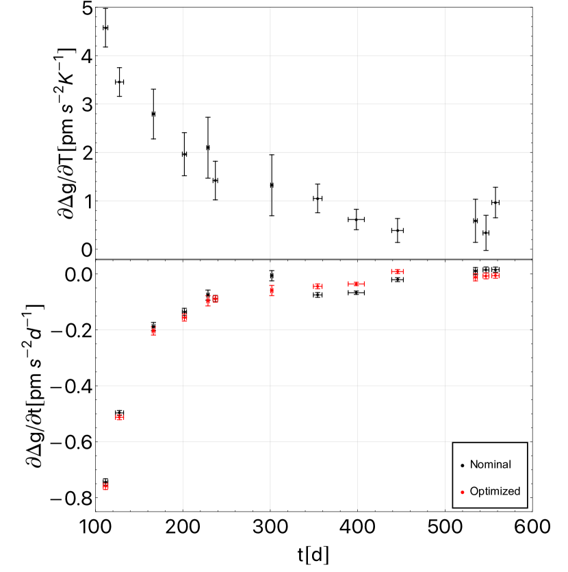
The relative rapid decay of both quantities in the early phase of the mission led us to investigate the existence of any possible correlation with the similar decay of Brownian noise.

We have found a quite significant linear relation between $\partial\Delta g/\partial T$ and $\partial S_{\text{Brown}}/\partial T$; we calculate the latter, from Sec. IV, as $\partial S_{\text{Brown}}/\partial T=(T_{a}/T^{2})S_{\text{Brown}}$ (see Fig. 12).

FIG. 12: $\partial\Delta g/\partial T$ vs $\partial S_{\text{Brown}}/\partial T$ for the nominal calibration. Points are the data while the dashed line is the linear, least square best fit $\partial\Delta g/\partial T=\alpha_{T}\;\partial S_{\text{Brown}}/\partial T$, with $\alpha_{T}=(1.49\pm 0.07)\times 10^{18}\,\text{s/m}$.

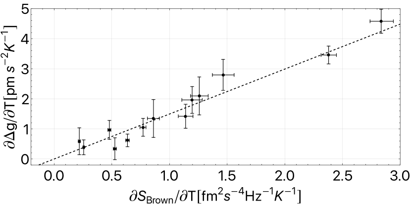
A fit with the simple proportionality relation $\partial\Delta g/\partial T=\alpha_{T}\partial S_{\text{Brown}}/\partial T$, gives $\alpha_{T}=(1.49\pm 0.07)\times 10^{18}\,\text{s/m}$ (see Fig. 12). The chi-squared test for the goodness of such fit gives $p=0.8$.

Note however that the factor $(T_{a}/T^{2})$ changes at most by some 6% from run to run, thus the correlation between $\partial\Delta g/\partial T$ and $S_{\text{Brown}}$ itself is as strong as the other. Nevertheless, we will continue to discuss the case for $\partial S_{\text{Brown}}/\partial T$ for reasons that will be clear in the following.

A plot of $\partial\Delta g/\partial t$ as a function of $S_{\text{Brown}}$ shows a rather low level of linear correlation. The linear correlation is instead rather significant between $\partial\Delta g/\partial t$ and $\partial S_{\text{Brown}}/\partial t=(-\gamma/(t-t_{v}))S_{\text{Brown}}$ (following from Eq. (5)). A plot is shown in Fig. 13 together with a best fit to the data with $\partial\Delta g/\partial t=\alpha_{t}\partial S_{\text{Brown}}/\partial t$ that gives $\alpha_{t}=(1.4\pm 0.2)\times 10^{18}\,\text{s/m}$.

FIG. 13: $\partial\Delta g/\partial t$ vs $\partial S_{\text{Brown}}/\partial t$. Black points are the data for the nominal calibration, and the black dashed line is the linear, least square best fit to the black points with $\partial\Delta g/\partial t=\alpha_{t}\partial S_{\text{Brown}}/\partial t$, and $\alpha_{t}=(1.4\pm 0.2)\times 10^{18}\leavevmode\nobreak\ \text{s/m}$. Red data and line have the same meaning, but for the optimized calibration. In this case $\alpha_{t}=(1.44\pm 0.07)\times 10^{18}\leavevmode\nobreak\ \text{s/m}$.

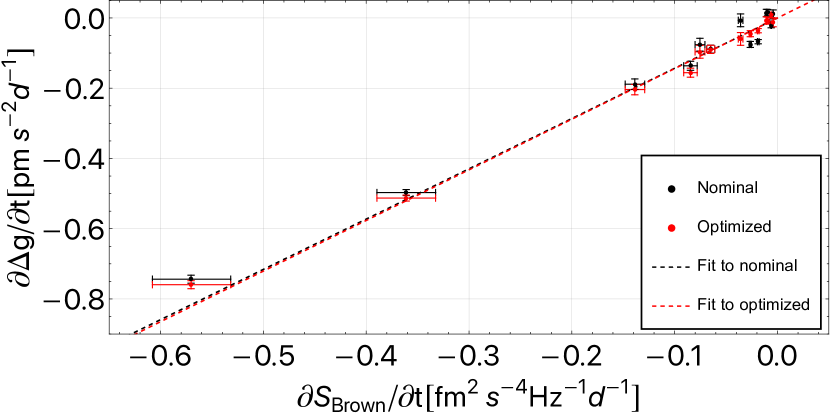
The goodness of the fit to nominal data is rather poor, with negligible $p$-value. As the gravitational drift is large, even a limited change to the values of $\omega_{d}^{2}$, $\kappa_{t,i}$ and $\kappa_{b,j}$, used for its subtraction, may change the value of the residual drift and then of $\partial\Delta g/\partial t$. Thus the uncertainty on those coefficients projects a large uncertainty on the true value of $\partial\Delta g/\partial t$, uncertainty that is not taken into account while performing the goodness of fit test.

To show that this is the case, we have searched if values of $\omega_{d}^{2}$, $\kappa_{t,i}$ and $\kappa_{b,j}$, other than the nominal ones, but still within the range of their uncertainties, may improve the quality of the fit. Actually, we have searched for the values that just give the maximum $p$-value in the goodness of fit test.

We find that the maximum is attained when $\kappa_{t,1}=1.00$, $\kappa_{t,2}=1.05$, $\kappa_{t,3}=0.95$, $\kappa_{b,A}=1.00$, $\kappa_{b,B}=0.92$, and $\omega_{d}^{2}=-3.31\times 10^{-7}\,\text{s}^{-2}$. With this ‘optimized’ calibration, $\alpha_{t}=(1.44\pm 0.07)\times 10^{18}\,\text{s/m}$, and the $p$-value is $p=0.18$ (See Fig. 13). Remarkably, moving to this optimized calibration, within errors, does not change the slope of the line.

The most important observation though, is that $\alpha_{T}=\alpha_{t}\equiv\alpha$ within the errors. This supports, with all the limitations and caveats that come from the empirical approach we had to use to process the data, that, for run $k$, the long-term evolution of $\Delta g$ obeys:

$$\Delta g_{k}(t)=\alpha S_{\text{Brown}}(t)+\Delta g_{0,k}=2\alpha\kappa P_{\text{H}_{2}\text{O}}+\Delta g_{0,k}$$ (11)

with $\Delta g_{0,k}$ a constant that depends on the run, and is affected by many operational factors that may be different in different runs.

In Eq. (11) we have used the conversion from Brownian noise PSD to the mean pressure around the TM that we have discussed in Sec. IV. It is interesting to note that also $\Delta g$ may be converted into an equivalent difference of pressure between the $x$-faces of one of the TM’s, as $\Delta P_{\text{H}_{2}\text{O}}=M\Delta g/L^{2}$, with $M$ the mass of the TM and $L$ the length of one of its edges. Then $\Delta P_{\text{H}_{2}\text{O}}=((2M\alpha\kappa)/L^{2})P_{\text{H}_{2}\text{O}}=(4.5\pm 0.2)\times 10^{-3}\,P_{\text{H}_{2}\text{O}}$. If the pressure difference was similar and opposite on both TM’s, not unlikely given the mirror symmetry of the instrument, then all figures should be divided by 2.

The temperature dependence of $\Delta g$ at these very low frequencies is consistent with the transient behavior of the lowest frequency datum reported in Fig. 9. Indeed a Bayesian decorrelation of temperature, following the method of App. B.3.2, gives the red points in Fig. 9, which show a suppressed initial transient, and a significantly reduced discrepancy from the $1/f$ tail.

Remarkably, the coefficient obtained from the decorrelation, $\left(\partial\Delta g_{e}/\partial T\right)_{\text{noise}}$, is in quantitative agreement with the values of $\partial\Delta g_{e}/\partial T$ reported in Fig. 12 (see Fig. 14). This confirms our modelization.

FIG. 14: Temperature coefficient $\left(\partial\Delta g_{e}/\partial T\right)_{\text{noise}}$ from the Bayesian temperature decorrelation of the lowest frequency datum, vs the temperature coefficient $\partial\Delta g_{e}/\partial T$ of Fig. 12. The dashed line is the result of a linear least square fit, which gives $\left(\partial\Delta g_{e}/\partial T\right)_{\text{noise}}=\left(1.0\pm 0.1\right)\partial\Delta g_{e}/\partial T+(-0.3\pm 0.2)\,\text{pm\,s}^{-2}\,\text{K}^{-1}$, with a reduced chi-square $\chi^{2}\simeq 0.6$.

We will discuss in Sec. VI the implication of such findings for the nature of the vacuum environment of the TMs.

VI Discussion I: Brownian noise, long-term drift, and the TM vacuum environment

In this and in the following section we discuss the physical information we can gather from the observation reported so far.

We start discussing the Brownian noise and the very low-frequency behavior, both drift and ASD, as both shed light on the nature of the vacuum environment surrounding the test mass.

We will discuss in some detail the possible physical sources of the $1/f$ tail in a following section.

VI.1 Brownian noise

Power-law evolution of pressure over time is very often observed in vacuum systems during initial pump down [27]. When the outgassing surfaces consist predominantly of metals, like stainless steel, aluminum, or titanium, a $\propto 1/t$ behavior is very often observed, consistent with models in which water vapor is in quasi-equilibrium between thermal outgassing from the metal walls, and re-adsorption onto them. To check if this model would be consistent also with our observed $\propto 1/t^{0.8}$ behavior, we have attempted to fit our observations to it. To this aim, we have integrated the differential equation (see [28])

$$\frac{1}{P}\frac{dP}{dt}=-\frac{\frac{1}{\tau}+\frac{P_{s}}{P}\frac{d\theta}{dT}\frac{dT}{dt}}{1+P_{s}\frac{d\theta}{dP}}$$ (12)

that, within such model, describes the time evolution of pressure. Here

• $\theta\left(P,T\right)$ is the fraction of occupied adsorption sites.

• $P_{s}=N_{s}k_{B}T/V$, with $N_{s}$ the total number of available adsorption sites, and $V$ the vacuum enclosure volume.

• $\tau$ is the vacuum relaxation time of the vacuum enclosure, in the absence of outgassing and adsorption, which is set by $V$ and by the pumping speed of the vent duct and is of the order of 0.2 s.

Eq. (12) can only be solved in combination with a choice for the functional form of $\theta\left(P,T\right)$. A versatile form that reproduces observations in many cases, is the Temkin isotherm [33].

$$\theta\left(P,T\right)=\frac{T}{T_{2}-T_{1}}\log\left(\frac{1+\frac{P}{P_{0}e^{-T_{2}/T}}}{1+\frac{P}{P_{0}e^{-T_{1}/T}}}\right)$$ (13)

With $P_{0}$, $T_{1}$ and $T_{2}$ free parameters of the model. We have done a least squares fit of the observed values of $S_{\text{Brown}}/(2\kappa)$ to the prediction of Eq. (12), as a function of $P_{s}$, $\tau$, $P_{0}$, $T_{1}$, and $T_{2}$. For each choice of the parameters we have integrated Eq. (12), and calculated the chi-square of the deviation of the data from the resulting solution. To integrate the equation, we have used the mean measured GRS temperature, mentioned before, throughout the entire integration time interval, except for the short duration epoch of the cold run, where we have used the proxy made with the LTP bay thermometers, also mentioned before.

The best-fit line is the dotted grey line in Fig. 3. The reduced chi-square of the minimum is rather poor $\simeq 2.0$, though this can be, at least in part, due to a significant underestimation of the true uncertainties in the model.

A more serious limitation with such an interpretation lies in the best-fit parameter values. Let us first mention that, provided $P_{0}\,e^{-T_{2}/T}\ll P\ll P_{0}\,e^{-T_{1}/T}$, the chi-square is found to depend only on $P_{0}$ and on the combination $c=(T_{2}-T_{1})/(\tau P_{s})$. Such a simplification can also be readily derived from an inspection of Eqs. 12 and 13. For these two parameters, the fit gives a broad minimum for $\log P_{0}$, $\log_{10}\left(P_{0}/$1\text{\,}\mathrm{k}\mathrm{P}\mathrm{a}$\right)=(1.4\pm 0.3)$, and a relatively narrow minimum for $c$, $c=(0.328\pm 0.004)\leavevmode\nobreak\ $\mathrm{K}\,\mathrm{d}^{-1}\,\mathrm{\SIUnitSymbolMicro}\mathrm{Pa}^{-1}$$.

The value for $P_{0}$, $P_{0}\simeq$25\text{\,}\mathrm{kPa}$\simeq$200\text{\,}\mathrm{T}\mathrm{o}\mathrm{r}\mathrm{r}$$ is orders of magnitude smaller than the quoted, for in instance, in [33] of about $6\times 10^{8}$ Torr, and within the theory discussed in that same reference, the only way to get such a small number would be to assume an unreasonably low density of adsorbing sites or an equally unreasonably high molecular attempt frequency.

Furthermore, of the four parameters that enter in the definition of $c$, $\tau$ can be independently evaluated from the estimated conductance of the vacuum valve and the vent duct, and from the volume of the vacuum enclosure, to be $\tau\simeq$0.3\text{\,}\mathrm{s}$$. A possible choice for the temperature values is given in [33], and is $T_{1}\simeq$5.3\text{\,}\mathrm{kK}$$ and $T_{2}\simeq$11\text{\,}\mathrm{kK}$$. The value for $T_{1}$ is only marginally fulfilling the condition on the pressure range. The closest value that still keeps the chi-square at its minimum is $T_{1}=$4.5\text{\,}\mathrm{kK}$$. With this choice for $\tau$, $T_{1}$, and $T_{2}$, we get $P_{S}=$6.0\pm 0.1\text{\,}\mathrm{kPa}$$. In turn, from this value for $P_{s}$, assuming, as in [33] a density of sites $\simeq 3\times 10^{15}\,\text{cm}^{-2}$, we get an estimate for the internal area of the vacuum enclosure of $\simeq 180\,\text{m}^{2}$, a couple of orders of magnitude larger than the physical area.

Thus to reconcile $P_{0}$ with the model one would need fewer absorption sites, while for $P_{s}$ one would need more. We believe that the chance that water re-adsorption has played a major role in our vacuum system is highly unlikely.

An alternative to the model of water desorption from walls, known to show as well power-law evolution over time, is diffusion-limited outgassing. In the case of hydrogen outgassing from stainless steel, for instance, a $1/\sqrt{t}$ evolution is often observed, in agreement with Fick’s law prediction for one-dimensional diffusion [28]. Approximate outgassing power-law evolution with an exponent even larger than 0.5 is observed in the presence of polymers and is attributed to water diffusion through them. In addition, experiments on polymer samples show that the temperature dependence of the outgassing rate is well described by a single activation exponential, as is the case of our observation [28].

Given the abundance of polymers in cable bundles, motors, and connectors within the GRS, and given in general the complex geometry of the TM surroundings with abundant solid interfaces, it looks rather likely that desorption from walls is playing a minor role, and that gas diffusion out of some of the GRS components is dominating the pressure environment.

VI.2 Long-term drift, very low frequency noise and pressure gradient

The results of Sec. V.6 support the idea that there was a permanent difference of pressure across one or both the TMs, whose amplitude scales with the overall pressure as measured by the Brownian noise level. This pressure gradient makes $\Delta g$ both sensitive to temperature, because of the corresponding temperature sensitivity of pressure, and drifting, because of the pressure drift due to venting to space.

We have simulated with Molflow+ [34] the effect of localized outgassing on the pressure on the TM. Simulations consistently show that, due to the rather complex geometry of the TM surroundings, which creates a rather asymmetric molecular flow impedance pattern, it takes very little asymmetry of outgassing to support a pressure gradient across the TM.

To give a scale of the phenomenon, a large fraction of any flow of molecules out of the cavity formed by the outer wall of the EH and the Tungsten balance mass (see Fig. 15 of Ref. [20]), penetrates inside the EH, through a hole in the EH $x$-wall, symmetric to that for the laser beam. These molecules diffuse in the gaps surrounding the TM and, in a time of the order of ms, eventually leave the EH. In their flow within the EH, these molecules exert both a mean pressure on the TM, and a pressure difference across the $x$-axis. We find that this difference is approximately 30% of the overall mean pressure contribution around the TM.

On the contrary, simulations show that outgassing from sources farther away from the EH, like, for instance, from the inner wall of the VE, diffuses and equalizes outside the EH and does not create any significant pressure difference across the TM.

VI.3 In summary: the vacuum environment of the TMs

The observed tight link between the total residual pressure, as measured by the Brownian noise level, and the decaying drift in $\Delta g$, with both time and temperature, implies, as a minimum, the same desorption properties for the gas setting the overall residual pressure and the pressure gradients.

The most simple explanation for this is that the dominant source of outgassing in the GRS is diffusion out of sources close to the TM, that is, located inside the EH or just outside its $x$-walls. These sources may include the electrodes, the insulators and the structure of the EH, the Tungsten balance mass, the cables placed close to the outer $x$-walls of the EH, and a few other elements.

This recommends, in preparation for LISA, to conduct in-depth qualification studies on the outgassing properties of these elements.

VII Discussion II: excess noise and possible observational artifacts

Here we begin discussing the possible sources of the observed $1/f$ tail. We first consider the role of some possible observational artifacts, while a detailed projection of the noise onto the possible modeled sources is discussed in the next section.

VII.1 Role of interferometer noise.

The contribution of interferometer noise $n_{\text{OMS}}$, with ASD $S_{n_{\text{OMS}}}^{1/2}$, to $S_{\Delta g}^{1/2}$ is $S_{\Delta g,n}^{1/2}=S_{n_{\text{OMS}}}^{1/2}\left(4\pi^{2}f^{2}+\lvert\omega_{2}^{2}\rvert\right)$.

Thus, for $f\leq\lvert\omega_{2}\rvert/2\pi$, a branch of $S_{n_{\text{OMS}}}^{1/2}$, raising rapidly enough upon decreasing frequency, may have contributed to $S_{\Delta g,e}^{1/2}$.

In our ordinary noise measurements, there was no way to separate $S_{\Delta g,n}^{1/2}$ from the contribution of true forces. We have however two independent methods to put an upper limit to the former.

The first method is to use the interferometer data we collected during an epoch in which the test masses were held fixed by the blocking mechanism [35]. This gave us the chance to measure the interferometer output noise in open loop, that is, with no active control of the TM positions, which is the quantity appearing in Eq. (2). The results for $S_{\Delta g,n}^{1/2}$ are reported in Fig. 15 and compared to the lowest $S_{\Delta g_{e}}^{1/2}$ data, that is those from run 10 of Table 1.

FIG. 15: Role of interferometer noise in the overall ASD of $\Delta g$: Red points: $S_{\Delta g_{e}}^{1/2}$ for run 10 (February 2017), as in Fig. 2. Dark blue points: $S_{\Delta g,n}^{1/2}$ measured with blocked TMs. Light blue points: ASD of the difference $\Delta g-\Delta g_{\text{GRS}}$ for run 10.

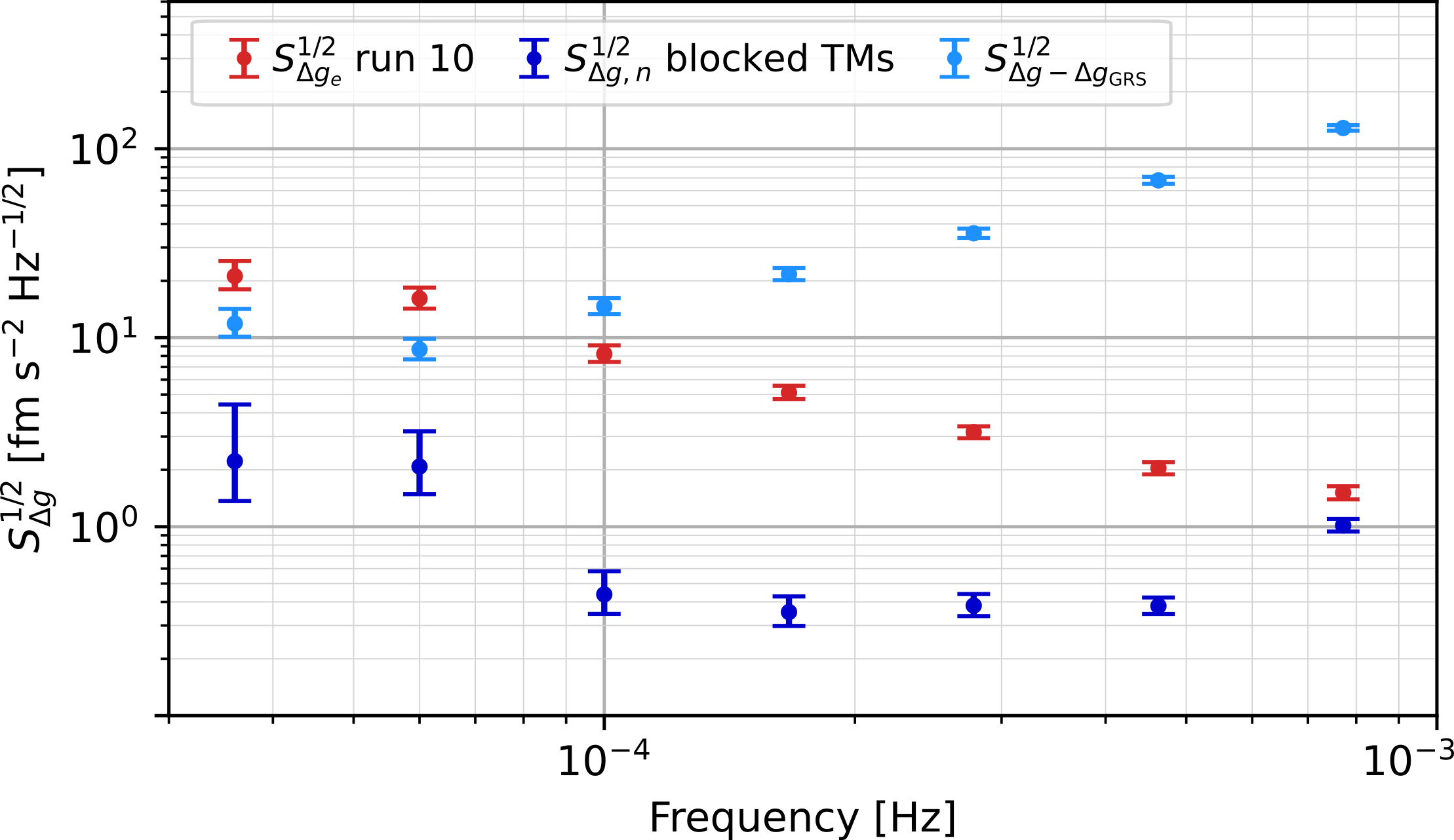
The second method exploits the independent capacitive measurement of the relative motion of the TMs $\Delta X_{\text{GRS}}$. As the ordinary $\Delta g$ is calculated using $\Delta X_{\text{OMS}}$, we can calculate the analogous $\Delta g_{\text{GRS}}$, using $\Delta X_{\text{GRS}}$. $\Delta g_{\text{GRS}}$ is significantly more noisy than $\Delta g$ at all frequencies above $80\text{\,}\mathrm{\SIUnitSymbolMicro Hz}$, while the agreement of $\Delta g$ and $\Delta g_{\text{GRS}}$ at lower frequencies, with their independent readouts, indicates that we are observing the true force noise.

Neglecting any distortion, the difference between the two is just $\Delta g-\Delta g_{\text{GRS}}=\lvert\omega_{2}^{2}\rvert\left(n_{\text{OMS}}-n_{\text{GRS}}\right)+\ddot{n}_{\text{OMS}}-\ddot{n}_{\text{GRS}}$, and the ASD of this difference is then $S_{\Delta g-\Delta g_{\text{GRS}}}^{1/2}=\left(\lvert\omega_{2}^{2}\rvert+(2\pi f)^{2}\right)\sqrt{S_{n_{\text{OMS}}}+S_{n_{\text{GRS}}}}$. This provides then an upper limit for $\left(\lvert\omega_{2}^{2}\rvert+(2\pi f)^{2}\right)S_{n_{\text{OMS}}}^{1/2}$. Note that $n_{\text{GRS}}$ is an all encompassing figure and includes not just electronic noise but also the spurious pickup of degrees of freedom other than $\Delta x$.

Figure 15 shows the values $S_{\Delta g-\Delta g_{\text{GRS}}}^{1/2}$ for run 10. It is worth to add that the values for $(\lvert\omega_{2}^{2}\rvert+(2\pi f)^{2})S_{\Delta X_{\text{GRS}}}^{1/2}\simeq(\lvert\omega_{2}^{2}\rvert+(2\pi f)^{2})S_{n_{\text{GRS}}}^{1/2}$, not shown in the figure, coincide almost exactly with those for $S_{\Delta g-\Delta g_{\text{GRS}}}^{1/2}$, which shows that the role of $n_{\text{OMS}}$ in these is negligible.

Both methods give an upper limit to the interferometer contribution, likely rather pessimistic. Indeed within the blocked TM measurement the contrast was poor and the interferometer performance at $f>10\,\text{mHz}$ was at least one order of magnitude worse than that with the free TMs. In addition, the interferometer output might still have included some residual relative motion of the TMs, due to any mechanical distortion of the instrument. On the other hand the data $S_{\Delta g-\Delta g_{\text{GRS}}}^{1/2}$ are clearly dominated by the GRS noise, with the noise from the interferometer, and the TM motion, not contributing more than 1% in power.

In conclusion we consider that measured with the TM fixed as the relevant upper limit on interferometry noise contribution to $\Delta g$, a contribution which is less than some 1-2% in power, and probably significantly less than this figure.

VII.2 Excess noise as a flow of undetected glitches

As soon as transient events, known as glitches, were observed in the data [20] and removed from them, the question arose if the excess noise might be due to an undetected and non-removed fraction of glitches. Not only is the question a legitimate one, but it is also made particularly relevant by the observation that both the glitch properties and the excess noise appeared rather stable throughout the mission, despite the changes in operation conditions [20].

We have addressed the question by performing extensive simulations. The detail of such simulation work is reported in App. G.

The basic conclusion is that the excess noise might be due to a Poisson flow of undetected glitches, but those glitches would belong to a distribution quite well separated in properties from that of the detected ones. In addition, the flow rate should be high enough that the resulting noise would be stationary and Gaussian, bearing no detectable feature proving its Poisson nature.

Thus if the $1/f$ tail is made of Poisson noise this is not related to the observed glitches, and its Poisson nature does not show up in the data.

VIII Discussion III: projection of excess noise on modeled noise sources

In this section, we estimate the contribution of modeled sources of force noise to the observed excess over the Brownian noise.

Our approach is to give a quantitative estimate of those contributions whenever they appear to be significantly different from zero, while we try to establish an upper limit whenever the resolution of our methods limits the estimate.

We focus our analysis on the run performed in February 2017, run 10 of Table 1, which is the lowest noise one. We will also discuss, whenever relevant, the case for the other runs.

We consider two categories of sources: the first includes the effect of physical quantities that have been measured during noise runs, synchronously with $\Delta g$; the second includes effects for which we have an estimate from different experiments, performed at different times from those of the noise runs.

For sources of the first category, we infer their contribution to the ASD of $\Delta g$ via a ‘decorrelation’ method. For those in the second category, we just give the best estimate of the contributed noise ASD.

VIII.1 Decorrelation of synchronous time series: framework

During noise runs we have measured, synchronously with $\Delta g$:

1. The gravitational force loss due to fuel depletion, $\Delta g_{\text{Tanks}}$ defined in Sec. V.6;

2. The relative motion of the two GRS, $\Delta X$, as defined in App. E;

3. Temperature $T$, defined in Sec. II.3;

4. The two temperature differences across the two electrode housings, in the $x$-direction;

5. The three magnetic field components at four different locations;

6. A series of spurious low-frequency voltages that have unintentionally been applied to the electrodes via the actuation circuitry non-linearity [19].

We treat these disturbances as small and Gaussian and consider their effect only to first order, within the simple model:

$$\begin{cases}\Delta g(t)&=\Delta g_{0}(t)+\sum_{i=1}^{r}\int_{0}^{\infty}\alpha_{i}(t^{\prime})y_{i}(t-t^{\prime})\mathrm{d}t^{\prime}\\ z_{i}(t)&=y_{i}(t)+n_{i}(t)\end{cases}$$ (14)

where $z_{i}(t)$ is any of the measured time series above, consisting of the “true” physical disturbance $y_{i}(t)$, superimposed to its readout noise $n_{i}(t)$. $\Delta g_{0}$ is the residual acceleration, not correlating to $y_{i}$.

Given the nature of the disturbances considered, the susceptibilities $\alpha_{i}(f)$, i.e. the Fourier transforms of the $\alpha_{i}(t)$, should be, for most of them, real and constant, but we also consider the general case to take into account the possibilities of delays and other more complex correlations.

With the model in Eq. (14), the elements of the cross-spectral density (CSPD) matrix $\bm{\Sigma}$ of $\Delta g$ and the $z_{i}$ are given by

$$\begin{split}&\Sigma_{1,1}=S_{\Delta g}(f)=S_{\Delta g_{0}}(f)+\sum_{i,j=1}^{r}\alpha_{i}(f)\alpha_{j}^{*}(f)S_{y_{i},y_{j}}(f)\\ &\Sigma_{i+1,1}=S_{y_{i},\Delta g}(f)=\sum_{j=1}^{r}\alpha_{j}^{*}(f)S_{y_{i},y_{j}}(f)\\ &\Sigma_{i+1,j+1}=S_{z_{i},z_{j}}(f)=S_{y_{i},y_{j}}(f)+\delta_{i,j}S_{n_{i}}(f)\end{split}$$ (15)

In Eq. (15), $S_{y_{i},y_{j}}(f)$ is the cross-spectral density between $y_{i}$ and $y_{j}$, while $S_{n_{i}}$ is the PSD of $n_{i}$. In all cases, except $\Delta X$ which we discuss separately, the readout noise $n_{i}$ is assumed to be independent of any of the other time series.

We deal with two broad cases. In the first case, we have an independent knowledge of the value of $\alpha_{i}(f)$, but we know or suspect that the readout noise $S_{n_{i}}(f)$ is significant, even dominating $S_{z_{i},z_{j}}(f)$. In the second case we have limited knowledge of $\alpha_{i}(f)$, but we are confident that $S_{n_{i}}(f)$ is negligible for the purpose of noise analysis. The general case of unknown susceptibilities and unknown readout noise is overdetermined and cannot be treated.

VIII.2 Decorrelation of synchronous time series: results for noisy series

VIII.2.1 Temperature effects and LTP distortion

The instrument distortion $\Delta X(t)$ and temperature $T(t)$ give rather significant contributions, $\Delta g_{\text{Dist}}(t)=\omega_{d}^{2}\Delta X(t)$, and $\Delta g_{T}(t)=\partial\Delta g/\partial T\times T(t)$, to the quasi-DC long-term evolution of $\Delta g$ (see Sec. V.6). In this section, we address their possible roles in contributing to the in-band excess noise, for $f\geq f_{2}$. As we found a significant correlation between these series [36], we consider them together.
Unfortunately, these two series are affected by a significant readout noise. Here briefly follows our knowledge of the properties of such noise.

Instrument distortion — The experimental PSD of $\Delta X$ peaks at about 0.1 mHz, and slowly decays above that [36]. The experimental CPSD between $\Delta X$ and $\Delta g$ parallels somewhat this behavior, its real part becoming significantly different from zero and positive above about 0.3 mHz, slowly decaying above that. In the frequency range in which the real part is significant, the imaginary part is also significantly different from zero, this time with a frequency-dependent sign. This behavior of the CPSD is hardly compatible with the gravitational signal from mechanical distortion, which is virtually instantaneous, and then free of imaginary CPSD, and supports instead the existence of a dominating readout noise of electrical origin.
Actually, the linear instrument distortion $\Delta X$ is the combination of four signals. Each of these signals consists of an independent differential capacitance measurement [6]. We find that only two of these signals bear some significant correlation with $\Delta g$, the correlation being in different frequency ranges for the two signals.
Both these signals refer to TM2, to whom the largest actuation is applied, and cross-correlation is likely due to electronic cross-talk between the actuation command signals and the TM motion sensing ones. At low frequencies the $\Delta g(t)$ time series is dominated by the actuation contribution $g_{c}(t)$ in Eq. (1), which brings an indirect correlation between $\Delta g$ and TM motion sensing within the GRS.

Analogously to the linear distortion $\Delta X$, the GRS allows to measure the angular distortion $\Delta\Phi\equiv\left(\Delta\phi_{\text{OMS}}-\Delta\phi_{\text{GRS}}\right)$, which is built with different combinations of the same four capacitance measurements. Once corrected with the analogous interferometer signal $\Delta\phi_{\text{OMS}}$, this signal measures the much suppressed angular distortion, while being insensitive to the linear one. Hence, it carries the same readout noise that affects $\Delta X$, though in a different combination. Including $\Delta\Phi$ in our model should lead to a better constraint of the contribution of these sources to $\Delta g$.

Temperature — The average temperature at the location of the test masses was measured by averaging the readings of various thermistors located on the external $x$-faces of the two electrode housings.
The time series of these thermistors were dominated, above about $\sim$30\text{\,}\mathrm{\SIUnitSymbolMicro Hz}$$, by excess electronic noise [8]. This fact was made particularly evident by the loss of mutual coherence among the time series of the different thermistors above that frequency, a coherence that below $\sim$30\text{\,}\mathrm{\SIUnitSymbolMicro Hz}$$ was nearly complete.
The noise was caused by a subtle interaction between drift and a nonlinearity of the analog-to-digital converter. For two of the eight available thermistors, such noise was so large that we had to discard the corresponding time series.

Regarding susceptibilities, we take those from the long-term behavior discussed in Sec. V.6. In addition, we measured the dependence of $\Delta X$ on $T$ by using the “low distortion” runs, that is by excluding run 7, 11, and 12 (see Sec. V.6). We find consistent results both by measuring the slope $\gamma=\partial\Delta X/\partial T$ in a linear fit over one-day-long data stretches, and from the CPSD between the two data series at $18\text{\,}\mathrm{\SIUnitSymbolMicro Hz}$. The distributions which we use for the susceptibilities are given in App. F. We recall here that $\omega_{d}^{2}$, $\alpha_{T}(f)$, and $\gamma(f)$ are, respectively, the susceptibilities of $(\Delta g,\Delta X)$, $(\Delta g,T)$, and $(\Delta X,T)$.

We address the problem with two different approaches, which are described in App. F.
The first approach is “naive”, as it assumes that the time series are not affected by any readout noise. It is represented as a dashed line in Fig. 16. The bound is completely dominated by the instrument distortion term, the effect of temperature alone being orders of magnitude smaller. However, it overcomes the entire excess noise above 0.1 mHz, resulting in a non-physical limit. Hence, this result carries no information.

FIG. 16: Upper bound ($1\sigma$) of the contribution of LTP distortion and of pressure-mediated temperature effect to $S_{\Delta g_{e}}^{1/2}$. Red data: ASD of the excess over Brownian $\Delta g_{e}$ from Sec. III. Dashed blue line: $1\sigma$ upper quantile of the estimate assuming time series free of readout noise, “naive” model. Solid blue line: $1\sigma$ upper quantile considering the presence of readout noise, as described in the text.

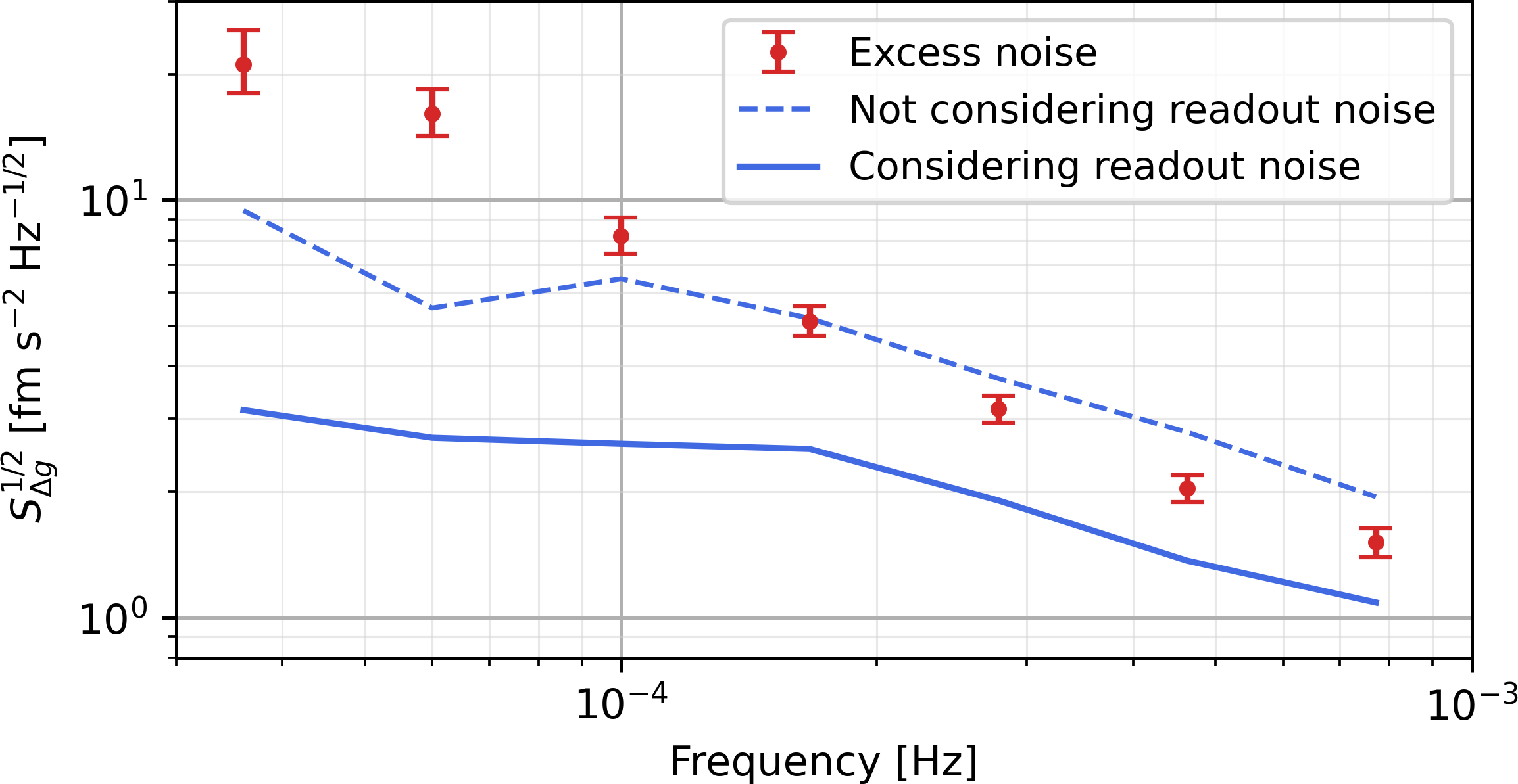
The second approach, on the contrary, is more refined as it takes into account that time series are affected by readout noises, possibly cross-correlating. Given the experimental assumptions on the susceptibilities, we model the contribution to $\Delta g$ of the time series $(\Delta X,T,\Delta\Phi)$, imposing that the residual noise matrix is positive-definite, as a CPSD matrix should always be. This way, we take into account that time series may be affected by readout noise. Details in App. F. The $1\sigma$ upper bound is reported in Fig. 16, solid line.

This upper limit is once again dominated by the effect of $\Delta X$, and constrained by its correlation with $\Delta\Phi$; the role of temperature is completely negligible. Despite being tighter than the “naive” one, this upper limit is still set by the large correlation between $\Delta g$ and the readout noise of $\Delta X$. Note that, as the temperature is irrelevant, the effect would amount to some non-thermal distortion of the LTP, such as long-term creep due to stress release. One would expect that, below the system mechanical resonances, all greater than $10\text{\,}\mathrm{H}\mathrm{z}$, the ASD of this kind of effects to be some, possibly rather steep power law of frequency [37]. But even for a $\propto f^{-1/2}$ dependence, the value of the limit at $f_{2}$, would set an upper limit at the highest frequencies at least a factor 4 in power smaller than that indicated by the solid line in Fig. 16. Thus this limit again probably significantly overestimates the effect.

Finally, note that this technique does not give an explicit lower limit, as the hypothesis that time series are constituted by readout noise only is fully compatible with the observations (solution $S_{X}=0$, $S_{T}=0$).

VIII.2.2 Tank depletion

The case for the gravitational signal from tank depletion is a bit easier than the previous one. However, here too the PSD of the readout noise of the propellant flow meter is unknown. The susceptibility is $\alpha_{\text{Tanks}}=\kappa_{t1}\kappa_{bB}$ (see Sec. V.6) a real, frequency-independent figure known to within a 10% uncertainty.

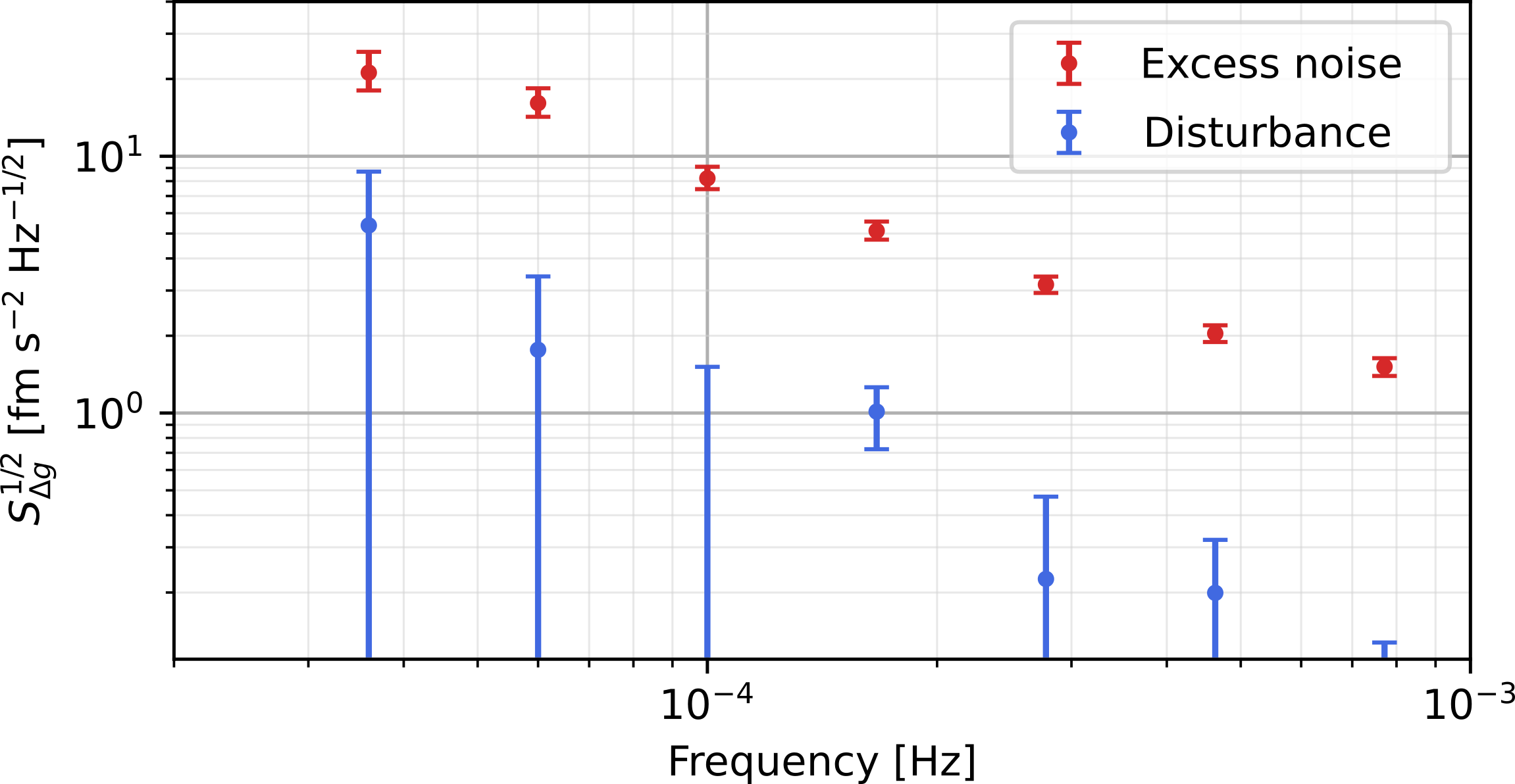
We estimate the contribution of this source of noise to the total excess noise as $\alpha_{\text{Tanks}}S_{\Delta g,\Delta g_{\text{Tanks}}}$, as explained in App. B.3.1, with $\Delta\tilde{g}_{\text{Tanks}}$ the true gravitational noise, free of any readout noise contamination.

We take the posterior for $S_{\Delta g,\Delta g_{\text{Tanks}}}$ from the proper Wishart distribution (see App. B.3.1), and that for $\alpha_{\text{Tanks}}$ to be a normal distribution with mean and standard deviation, respectively, 0.92 and 0.10 (see Sec. V.6). Results are shown in Fig. 17.

FIG. 17: Contribution of gravitational noise due to tank depletion to the ASD of $\Delta g_{e}$. Red data: ASD of the excess over Brownian $\Delta{g_{e}}$ from Sec. III. Blue data: $\pm 1\sigma$ posterior interval for the gravitational noise contribution from CPSD and susceptibility posteriors.

Note that $\sum_{i,j=1}^{r}\alpha_{i}(f)\alpha_{j}^{*}(f)S_{y_{i},y_{j}}(f)$ is a positive real number, while there is no guarantee that a posterior sample for $\sum_{i=1}^{r}\alpha_{i}(f)S_{y_{i},\Delta g}(f)$ is even real.

We have dealt with this problem in two ways. We have first checked that the posterior distribution of the imaginary part of $\sum_{i=1}^{r}\alpha_{i}(f)S_{y_{i},\Delta g}(f)$ was statistically compatible with zero.

We have then taken the posterior just for the real part of $\sum_{i=1}^{r}\alpha_{i}(f)S_{y_{i},\Delta g}(f)$, checking that, whenever the distribution extended to negative values, the zero was within the $\pm 1\sigma$ credible interval.

Except for the lowest frequency, the $+1\sigma$ limit is well below 10% in power. At the opposite end, except for one frequency, zero falls always within the $\pm 1\sigma$ interval.

VIII.3 Decorrelation of synchronous time series: results for series with negligible readout noise

For the time series we analyze here, we have limited prior knowledge about the susceptibilities, except that they are real and frequency-independent. This because delays between the time series and the forces they exert on the TMs are negligible.

We do then a simultaneous Bayesian fit at all frequencies as explained in App. B.3.2. This way we get a posterior for the residual $S_{\Delta g_{0}}(f)$, for the susceptibilities $\alpha_{i}$, and for the joint contribution to $S_{\Delta g}$, $S_{c}(f)=\sum_{i,j=1}^{r}\alpha_{i}\alpha_{j}S_{y_{i},y_{j}}(f)$ (see Eq. (15)).

$S_{c}(f)$ may be subject to a large positive bias in case of large $r$. For that reason we calibrate the method with extensive simulations, as explained again in App. B.3.2.

VIII.3.1 Spurious actuation due to in-band noise from digitized electrostatic actuation

The capacitive actuation design employed digitally-synthesized audio-frequency sinusoidal voltages [19]. As the force is quadratic in the voltage, this applies a force at low frequency, proportional to the mean square value of the sinusoid, while avoiding mixing down low-frequency voltage noise from the final amplifiers.

The truncation error mentioned earlier affects the above mean square value, and, if uncorrected, gives a wrong estimate of the applied force.

The nominal sinusoidal voltage signal has zero time average and then zero dc value. The truncated signal acquires a non-zero average, that is a quasi-dc voltages $\delta V_{i}(t)$ of order $\sim$\mathrm{\SIUnitSymbolMicro V}$$ amplitude that we were able to calculate from the commanded voltages with negligible numerical noise.

These voltages are able to apply electrostatic forces onto the test masses by coupling to its charge and to the parasitic voltages biasing the electrodes [38]. To linear terms in the $\delta V_{i}(t)$’s this force is given by:

$$\Delta g_{D}(t)=\sum_{i\in[1,24]}\alpha_{i}\delta V_{i}(t)$$ (16)

where the sum is over the 24 electrodes that surround the two TMs, and where the susceptibility $\alpha_{i}$ is a linear combination of charge and patch potentials, and cannot be predicted except, possibly, in order of magnitude.

In reality, due to cosmic rays, the TM charge is subject to an approximately linear variation in time, $q(t)\sim q_{0}+\dot{q}t$ [21], with $\dot{q}\sim+23\leavevmode\nobreak\ $\mathrm{e}\mathrm{/}\mathrm{s}$$. On the charge itself the relative effect may be large, as we have often operated by putting a proper negative charge on both TMs at the beginning of a noise run, to find an equal but opposite charge on them at the end of the run.

Hence, a complete analysis should in principle include 48 charge parameters. To circumvent this problem, we have taken advantage of the fact that the differential force contribution due to the coupling of the $\delta V_{i}(t)$ to the drifting charge is $\left(\dot{q}_{2}t\Delta_{x,2}-\dot{q}_{1}t\Delta_{x,1}\right)$. Here $\Delta_{x,i}$ is linear combination, with $\pm 1$ coefficients, of the $\delta V_{i}(t)$ of the $x$-electrodes of GRS$i$, as defined in [38], and $\dot{q}_{i}$ is the charging rate of TM$i$ [38].

We have then formed the two time series $t\Delta_{x,1}(t)$ and $t\Delta_{x,2}(t)$ and added them to our analysis. This obviously breaks the hypothesis of noise stationarity, but should still help highlight the existence of significant correlation.

To keep $r$ not too large, we have done two separate analyses. In the first we have included the 24 voltage series only. Note that with $r=24$ the analysis could only be performed for $f\geq f_{4}$ ($0.1\text{\,}\mathrm{mHz}$) as lower frequencies would not have a sufficient number of periodograms (see App. B.3.2).

In the second we have considered the two series $t\Delta_{x,1}(t)$ and $t\Delta_{x,2}(t)$, but we have also added the two series $\Delta_{x,1}(t)$ and $\Delta_{x,2}(t)$, to consider the complete effect of the charge, and to reduce the bias due to direct correlation between $\Delta g$ and the $\delta V_{i}(t)$ involved in the $\Delta_{x,i}$. This allows us to include just 4 signal time series, hence being able to analyze a wider set of frequencies. We show in Fig. 18 the results of the second analysis.

FIG. 18: Decorrelation of the coupling of spurious actuation to TM charging for run 10, over the [$0.036\text{\,}\mathrm{m}\mathrm{H}\mathrm{z}$, $0.77\text{\,}\mathrm{m}\mathrm{H}\mathrm{z}$] frequency band. Frequencies are slightly shifted for clarity. Grey points: ASD of total excess noise over Brownian, $S_{\Delta g_{e}}^{1/2}$, as in Fig. 2. Red points: Bayesian posterior $\pm 1\sigma$ interval for the residual ASD after decorrelation of the spurious actuation along the x axis. Blue points: estimated ASD $S_{c}^{1/2}$ of the contribution of spurious actuation along the $x$-axis.

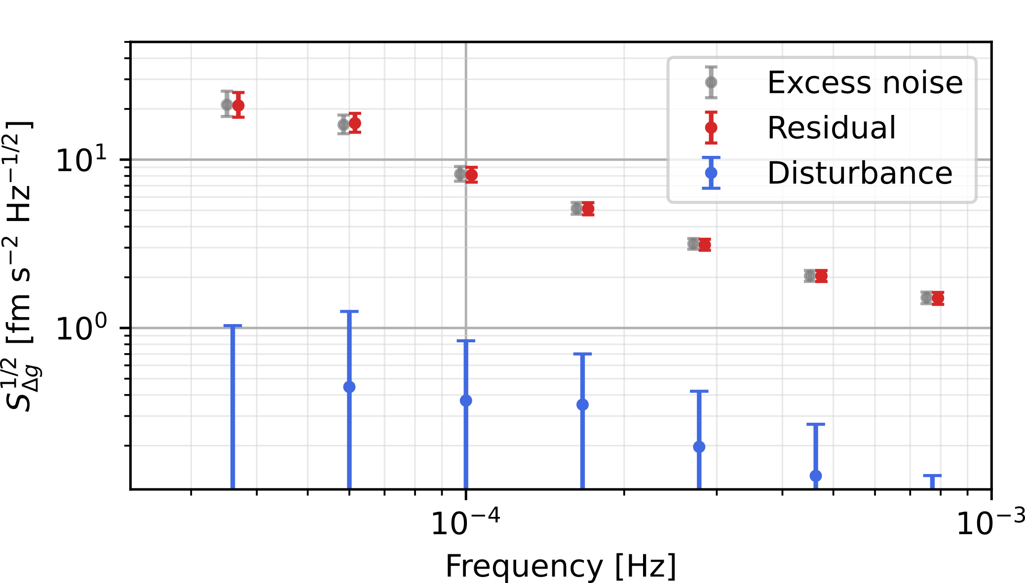
The results of Fig. 18 clearly show that this effect is compatible with zero within the resolution of the measurement. The $1\sigma$ error, on the other hand, is compatible with a contribution slightly less than $\simeq 1\%$ of total power at $f\geq f_{5}$, and much less below that. A similar result is obtained from the analysis of the 24 voltage series.

The posteriors of the susceptibilities are all compatible with zero, except, perhaps, for one. More specifically we have analyzed, for all the 24 $\alpha_{i}$, the likelihood, that we call $\mathcal{L}_{0}$, assigned by the posterior to the less likely of the two tails $\alpha_{i}<0$ and $\alpha_{i}>0$, as a very low likelihood of one of the two tails would indicate that $\alpha_{i}$ has a well-defined sign. All likelihoods are found to be larger than 5%, except for one, the voltage applied to one of the $x$-electrodes of TM1, which is $\mathcal{L}_{0}\simeq 1\%$. For this last series the susceptibility is $\alpha=(10\pm 5)\text{ fm s}^{-2}/\text{mV}$. To give an order of magnitude, if the coupling was due to a uniform stray voltage on the said electrode, this should be $(0.07\pm 0.03)\,\text{V}$, a figure in the range of observed patch potentials [38].

This slightly significant susceptibility is reflected, in the analysis with a linearly drifting charge, in an equivalently significant susceptibility to $\Delta_{x,1}(t)$, that contains the series above, while the susceptibilities to $t\Delta_{x,1}(t)$ and $t\Delta_{x,2}(t)$ are, within their large uncertainty, both compatible with zero and with the observed values of the charging rates [22].

VIII.3.2 Magnetic Fields

Below $\sim$1\text{\,}\mathrm{m}\mathrm{H}\mathrm{z}$$, the noise part of our magnetometer signals, as shown by their almost complete cross-correlation, and by the absence of any measurable fluctuating gradient [7], was dominated by the interplanetary magnetic field and had negligible readout noise. Because of their negligible gradient, the interplanetary field fluctuations interact with the TMs only as they induce, via the TM residual diamagnetism, a fluctuating magnetic moment that couples to any static magnetic field gradient at the TM location. The force due to this interaction is given by:

$$\Delta g(t)=\frac{\chi L^{3}}{M\mu_{0}}\left(\bm{\nabla}B_{x,\text{DC,2}}-\bm{\nabla}B_{x,\text{DC,1}}\right)\cdot\bm{B}(t),$$ (17)

where $\bm{\nabla}B_{x,\text{DC},i}$ is the magnetic gradient of the static $B_{x}$ component averaged over the volume of TM_i, $\mu_{0}$ is the vacuum magnetic permeability, and $\chi=(-3.37\pm 0.15)\times 10^{-5}$ the magnetic susceptibility of the test masses [39, 40].

Note that the static magnetic gradient may be different from the value that can be extrapolated, at the test mass location, from the differences of the magnetometer readings, which typically is $\simeq$0.5\text{\,}\mathrm{\SIUnitSymbolMicro}\mathrm{T}\mathrm{/}\mathrm{m}$$. Indeed a gradient up to $10\text{\,}\mathrm{\SIUnitSymbolMicro}\mathrm{T}\mathrm{/}\mathrm{m}$, is expected to be created by a series of thermistors, containing ferromagnetic materials, placed on the outer surface of the EH.

These thermistors are too far away from the magnetometers to give any significant measurable signal. Thus we had no in-flight information on the gradient that these thermistors were creating at the location of both TMs. A dedicated, in-flight experiment using oscillating magnetic fields [40] was able to give an estimate just for $\partial_{x}B_{x,\text{DC},1}$, that is, just for one of the three required components of the static magnetic gradient and at the location of just one of the TMs.

This lack of knowledge of the static magnetic gradient difference at the TM locations left us with only a possible order of magnitude estimate of the corresponding susceptibilities. Hence, we have performed our decorrelation analysis with no prior assumptions on the susceptibilities. The results are shown in Fig. 19.

FIG. 19: Decorrelation of low frequency magnetic fields for run 10, over the [$36\text{\,}\mathrm{\SIUnitSymbolMicro Hz}$, $0.77\text{\,}\mathrm{m}\mathrm{H}\mathrm{z}$] frequency band. Frequencies are slightly shifted for clarity. Grey points: ASD of total excess noise over Brownian, $S_{\Delta g_{e}}^{1/2}$, as in Fig. 2. Red points: Bayesian posterior $\pm 1\sigma$ interval for the residual ASD after decorrelation of the 3 magnetic field time series. Blue points: estimated ASD $S_{c}^{1/2}$ of the contribution of magnetic fields to $\Delta g_{e}$.

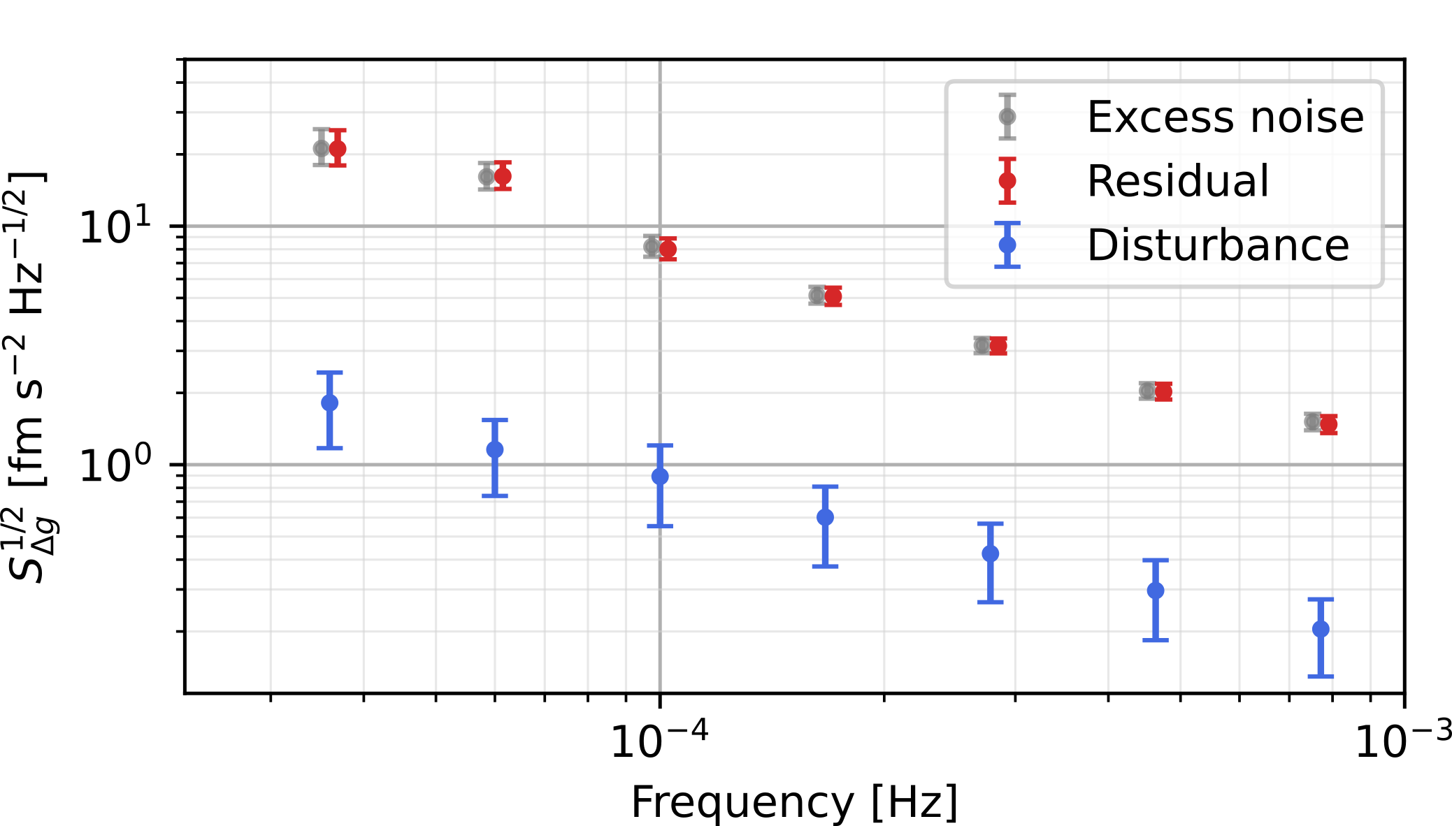
At all frequencies, $S_{c}(f)$ is significant at $1\sigma$, while the lower $2\sigma$ quantile of the posterior is negative.
Some significance is also supported by the susceptibilities. In particular, while $\mathcal{L}_{0}\geq 0.16$ for the $x$ and $z$ components of the field, $\mathcal{L}_{0}\simeq 0.001$ for the $y$ component. The corresponding susceptibility is $\alpha_{y}=(-8\pm 2)\,$\mathrm{f}\mathrm{m}\,\mathrm{s}^{-2}\mathrm{/}\mathrm{\SIUnitSymbolMicro}\mathrm{T}$$, that, if due to a gradient acting on just one of the two TMs, would correspond to $\lvert\delta\partial_{y}B_{x,\text{DC}}\rvert=(6\pm 2)\,$\mathrm{\SIUnitSymbolMicro}\mathrm{T}\mathrm{/}\mathrm{m}$$, close to what one would expect because of the magnetic thermistors [40]. The $\delta$ is meant to highlight that the measured quantity is the difference of magnetic gradients at the two TM locations.

We note that our estimate of the magnetic force noise ASD, based on decorrelation, is consistent with that reported in [39], which is based instead on a calculation from measured or estimated values of all the involved quantities. In particular, besides the in-flight measurements of the magnetic field fluctuations, that we also use, Ref. [39] uses the aforementioned measured value for $\partial_{x}B_{x,\text{DC},1}$, while the other components of $\bm{\nabla}B_{x,\text{DC,}i}$ are estimated based on a model for the statistical distribution of the magnetic dipoles associated with above mentioned thermistors.

VIII.3.3 Thermal gradients

In addition to single thermistor readout, that we used to form the average temperature signal, we also had two differential readouts, one for each GRS, each reading a pair of the thermistors located on the opposite faces of the EH of the corresponding GRS.

As the drift, which was the source of extra noise on the single readouts, is largely common mode among the thermistors , these channels were basically immune to the nonlinearity noise that plagued the average temperature, and fall then in the category of negligible noise time series.

Thermal gradients are the source of various forces, dominating ones being radiometer effect and asymmetric outgassing [41]. While for the radiometer effect the susceptibility can be estimated to within some 30%, $\alpha_{R}\simeq 2\times 10^{3}\,$\mathrm{f}\mathrm{m}\,\mathrm{s}^{-2}\mathrm{/}\mathrm{K}$$, for asymmetric outgassing the uncertainty is much larger [41], not better than an order of magnitude. The results of the decorrelation procedure are shown in Fig. 20.

FIG. 20: Decorrelation of thermal gradients for run 10, over the [$36\text{\,}\mathrm{\SIUnitSymbolMicro Hz}$, $0.77\text{\,}\mathrm{m}\mathrm{H}\mathrm{z}$] frequency band. Frequencies are slightly shifted for clarity. Grey points: ASD of total excess noise over Brownian, $S_{\Delta g_{e}}^{1/2}$, as in Fig. 2. Red points: Bayesian posterior $\pm 1\sigma$ interval for the residual ASD after decorrelation of the 2 thermal gradients time series. Blue points: estimated ASD $S_{c}^{1/2}$ of the contribution of thermal gradients to $\Delta g_{e}$.

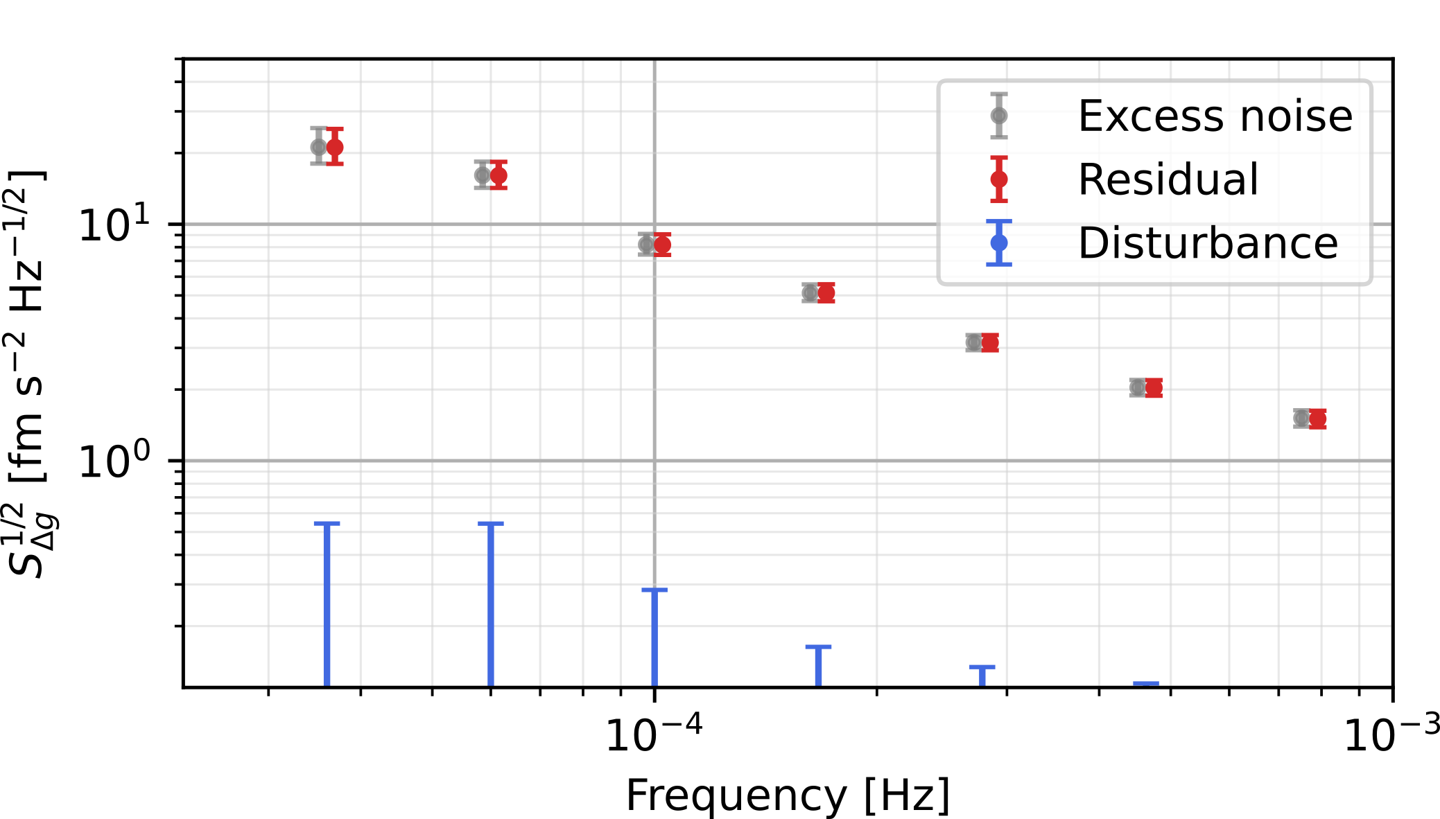
This contribution is clearly undetectable. Note that the susceptibilities, $(1\pm 5)\times 10^{3}\text{ fm s}^{-2}/\text{K}$, and $(1\pm 7)\times 10^{3}\text{ fm s}^{-2}/\text{K}$, are zero within errors, errors that comfortably include the value expected of the radiometric effect. This lack of contribution is due substantially to the good stability of the thermal gradient, with an ASD in the considered range of $\simeq$40\text{\,}\mathrm{\SIUnitSymbolMicro K}$/\sqrt{\text{Hz}}\sqrt{0.1\,\text{mHz}\,/\,f}$.

VIII.4 Modeled contributions from different experiments

As said, besides the disturbances discussed in the previous section, there is another set of effects that we could estimate from dedicated measurements separated from the noise measurements. The results of these experiments have been published in dedicated publications [22, 32, 42]. We list these disturbances in the following and use the results from those experiments.

• Actuation gain noise. This is the largest known contribution to the LPF noise in $\Delta g_{e}$. It consists of the effect of the gain fluctuations of the amplifiers that apply the audio-frequency actuation voltages to the TMs. During LPF operations we performed an extensive experimental campaign to model this force. The details of the measurements, and of their results are the subject of a dedicated paper [32]. In Fig. 21, blue points, we report from [32] the $\pm 1\sigma$ credible interval of the posterior for its contribution to $S_{\Delta g}$. Note that gain fluctuations also affect rotational actuation [32], and induce a correlation between $\Delta g$ and $\Delta\gamma_{\phi}$. The figures in Fig. 21 are in agreement with the effective cross-talk arm discussed in Sec. V.4.

• In-band voltage noise. Actuation voltage fluctuations within the measurement frequency band induce noisy forces on the test masses by coupling to their dc counterparts. Results of the measurements on this effect performed during LPF operations can also be found in [32], and reported again in Fig. 21 as orange points.

• Random charging. The effect of noisy charging due to cosmic rays was estimated, in [22], to be in quantitative agreement with an equivalent Poisson flow of single elementary charges arriving at a rate $\lambda_{\text{eff}}\sim 1\times 10^{3}\text{ s}^{-1}$. This Poisson charge flow converts into a force noise through the effective dc-voltage across the TM electrode capacitor system $\Delta_{x}$, as described in Ref. [22]. Considering residual dc-voltages – after compensation as in Table 5 – of $|\Delta_{x,1}|\sim|\Delta_{x,2}|\sim$5\text{\,}\mathrm{m}\mathrm{V}$$, the effect of random charging noise is shown as brown points in Fig. 21.

• Laser radiation pressure Fluctuation of the radiation pressure of the measurement laser beam induces a differential force on the TMs. The measurement beam reflects off TM1 and TM2, with nominal power $P_{1}=$2.4\text{\,}\mathrm{m}\mathrm{W}$$ and $P_{2}=$1.2\text{\,}\mathrm{m}\mathrm{W}$$ respectively. Relative fluctuations $\delta P_{1}/P_{1}$ and $\delta P_{2}/P_{2}$ induce a force $\Delta g\simeq$8\text{\,}\mathrm{p}\mathrm{m}\,\mathrm{s}^{-2}$\,(\delta P_{1}/P_{1})+$4\text{\,}\mathrm{p}\mathrm{m}\,\mathrm{s}^{-2}$\,(\delta P_{2}/P_{2})$. Unfortunately, on LPF there was no direct measurement of the instantaneous total optical power reflected off the test masses. However, [42] proposes a thorough analysis of the range of values of the contribution of this phenomenon to $S_{\Delta g}$. The analysis gets two possible estimates depending on the (unknown) sign of the correlation between different light polarizations. In Fig. 21 (green points) we report the overall range spanned by the $\pm 1\sigma$ uncertainty of both options.

FIG. 21: Estimated contributions to acceleration noise, for run 10 and within the [$36\text{\,}\mathrm{\SIUnitSymbolMicro Hz}$, $0.77\text{\,}\mathrm{m}\mathrm{H}\mathrm{z}$] frequency band, of: actuation gain fluctuations (blue points, data adapted from [32]); in-band voltage fluctuations (orange points, data adapted from [32]); cosmic ray charging fluctuations (brown points, estimate taken from [22]); laser radiation pressure fluctuations (green points, data adapted from [42]). For reference, we also report the ASD of the excess noise over Brownian $S_{\Delta g_{e}}^{1/2}$ as in Fig. 2, red points.

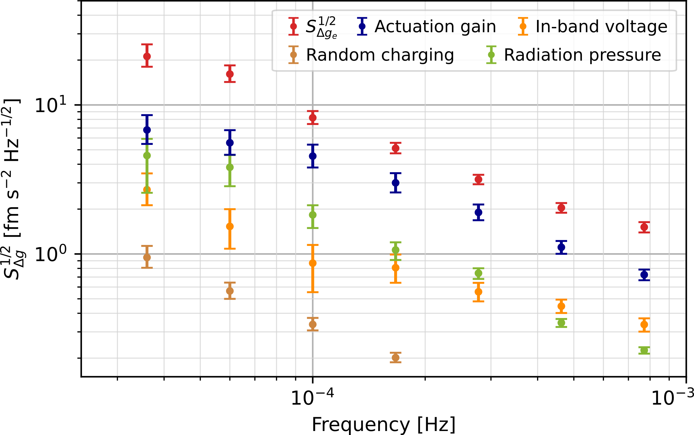
VIII.5 Summary of modeled contributions to excess noise

In Fig. 22 we report the ASD of the sum $S_{c,\text{tot}}$ of all contributions to the excess over Brownian $S_{\Delta g_{e}}$ that we have found to be, at least at some frequency in the [$36\text{\,}\mathrm{\SIUnitSymbolMicro Hz}$, $0.77\text{\,}\mathrm{m}\mathrm{H}\mathrm{z}$] band, statistically different from zero: tank depletion gravitational noise, magnetic fields, actuation gain fluctuations (that dominates the sum), in-band voltage fluctuations, random charging, and laser radiation pressure.

FIG. 22: Total modeled contributions to $S_{\Delta g_{e}}^{1/2}$, for run 10 in the [$36\text{\,}\mathrm{\SIUnitSymbolMicro Hz}$, $0.77\text{\,}\mathrm{m}\mathrm{H}\mathrm{z}$] frequency band. Red points: ASD $S_{\Delta g_{e}}^{1/2}$ of excess over Brownian. Dark blue points: modeled contributions $S_{c,\text{tot}}^{1/2}$, as described in the text. Light brown points: posterior for difference $\sqrt{S_{\Delta g_{e}}-S_{c,\text{tot}}}$. The dashed line is the best fit to the difference with exponent $n=1.00$, $\sqrt{S_{\Delta g_{e}}-S_{c,\text{tot}}}=$0.67\text{\,}\mathrm{f}\mathrm{m}\,\mathrm{s}^{-2}\mathrm{/}\sqrt{\text{Hz}}$\,($1\text{\,}\mathrm{mHz}$/f)^{1.00}$.

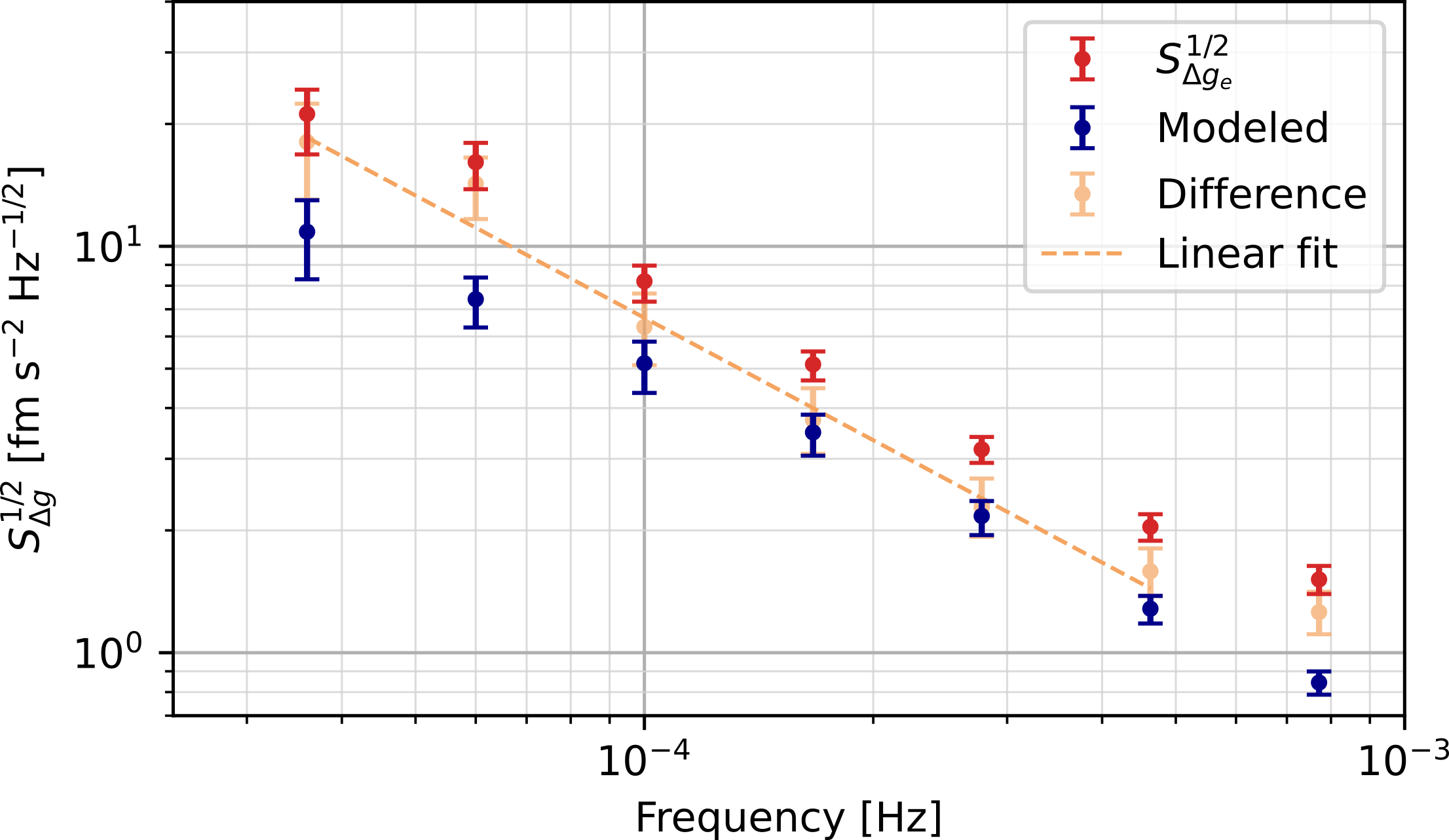
We have built the posterior for $S_{c,\text{tot}}$, by adding, whenever available, the samples of the $S_{c}$ posteriors of the various disturbances. For random charging and laser radiation pressure, for which we only had an error interval, we have assumed a Gaussian distribution with the $\pm 1\sigma$ interval coinciding with the said error one. Given the smallness of their contributions, the results are largely independent of the specific choice of such an equivalent posterior.

From the posterior for $S_{c,\text{tot}}$ and that for $S_{\Delta g_{e}}$, we have built that for their difference, our best estimate of the residual noise after subtraction of the effect of all modeled disturbances listed above. The results are shown again in Fig. 22 as the ASD $\sqrt{S_{\Delta g_{e}}-S_{c,\text{tot}}}$.

Such an ASD can be fit, in the range $36\mu\text{Hz}\leq f\leq 460\mu\text{Hz}$ to a power law $\widetilde{S}_{0}^{1/2}(1\,\text{mHz}/f)$ (see Fig. 22), with $\widetilde{S}_{0}^{1/2}=(0.67\pm 0.05)\,\text{fm\,s}^{-2}/\sqrt{\text{Hz}}$ and a reduced chi-square $\simeq 1$, which allows a direct comparison with the value of $\widetilde{S}_{\Delta g_{e}}^{1/2}$ (see Sec. V.2) for run 10, of $\widetilde{S}_{\Delta g_{e}}^{1/2}=(0.91\pm 0.04)\,\text{fm s}^{-2}/\sqrt{\text{Hz}}$. The ratio of their square, $\widetilde{S}_{0}/\widetilde{S}_{\Delta g_{e}}=(0.54\pm 0.09)$ gives the fraction of noise power that remains unexplained after our noise projection, the basic result of the procedure.

We have repeated our decorrelation procedure for the other runs, in order to assess if some of the observed variability of $\widetilde{S}_{\Delta g_{e}}$ (see Fig. 5) might be due to corresponding variations of some of the considered disturbances, and we could not find any evidence of that.

Among the disturbances in Sec. VIII.4, actuation gain fluctuations are the dominating ones. Unfortunately, we cannot assess the variability of those sources, as they were all determined in dedicated experiments. To justify the observed 20% variability of $\widetilde{S}_{\Delta g_{e}}$ by a corresponding variability of those, the latter should be of order 50%.

On the opposite end, if the entire variability is due to the 55% unjustified fraction, this should fluctuate by some 40%.

Finally, we have not included, in the above analysis, the contributions that we have found to be compatible with zero: LTP distortion, spurious actuation, and thermal gradients. While the addition of the latest two would not change the results in any appreciable way, the case of the distortion is different. Actually, the sum of the $+1\sigma$ value of $S_{c,\text{tot}}$ in Fig. 22 and the $1\sigma$ limit for $S_{c,\text{tot}}$ of Fig. 16, falls within $\pm 1\sigma$ credible interval of $S_{\Delta g_{e}}$ for $f\geq f_{5}$.

As said in Sec. VIII.2.1, however, this limit is likely to be significantly overestimated. The argument discussed in Sec. VIII.2.1, for instance, would reduce this contribution to no more than some 10% in power at the highest frequencies.

IX The unexplained excess: possible sources and implications for LISA

The previous section concludes that $(0.54\pm 0.09)$ of the measured excess noise remains unexplained by the sources for which we had a quantitative estimate. In this section we discuss the most likely sources of this unexplained fraction, and the measures one can possibly take to ensure that they do not compromise LISA performance.

IX.1 Patch potential fluctuations

Patch potentials [43] may cause force noise in many ways [38]: through the interaction of their time fluctuations with any static potential applied to the TM, including that due to the TM charge; by creating a quasi-static potential difference that may interact with electronic noise and charge fluctuations; through the interaction of their quasi-static part with their own fluctuations.

The first two effects have already been discussed in Sect. VIII.4. An analysis of the third effect, the self-interaction of the patch fields [44], also based on the results of the experiments with charge bias [32] in LPF, has appeared recently. The analysis indicates contamination as the most likely source of patches, and shows that a model of diffusion-driven fluctuations of contaminant density, that has been considered to explain self-heating in ion traps [45], may indeed predict force noise with $\propto 1/f^{2}$ PSD, with an amplitude in the range of the observed excess, for model parameter values that are not unreasonable.

Though such scenario remains unproven, its possibility would suggest a few precautions to be followed in the development of LISA. These have been discussed in [44], and we report them here for convenience.

First, torsion pendulum experiments with LISA-like TM have achieved sensitivities [38, 46] that may allow a direct detection of, or a significant upper limit to the noise we are discussing here. This would require though to reduce the gaps around the TM to around 1 mm or smaller. Needless to say, a direct measurement would bring this potential source of noise under full control.

In the absence of a direct measurement, a measure of precaution is to investigate the nature and the extent of the adsorbate that may have been present on the surface of LPF TM and EH during its operations. The objective is that of keeping TM contamination in LISA close to, or better than that in LPF.

This requires a campaign of surface characterisation on samples that have undergone a similar preparation history to that of LPF test masses. A systematic experimental study, with the Kelvin probe technique, of the quasi-static distribution of patch potentials, would be an important part of such a characterisation campaign.

It is reasonable to assume that if no new contaminants are introduced in LISA, that had not been present in LPF, and if the amount of contamination can be kept below that of LPF, the noise performance of LPF, that fulfills LISA requirements, may confidently be reproduced.

IX.2 Actuation force calibration and additional voltage noise

An obvious source of excess noise could be an inaccuracy in the calibration of the applied forces $g_{c}(t)$, which dominate the spectrum at sub-mHz frequencies; similarly, unaccounted nonlinearities in the applied voltages time series could lead to inaccuracies in the applied forces time series. Experiments were carried out in flight to calibrate the actuation system, against differences between commanded and applied forces/torques. In particular [18, 32], sinusoidal “calibration tones” of amplitude $100\text{\,}\mathrm{fN}$ and frequency $10\text{\,}\mathrm{mHz}$ were injected out-of-loop, effectively inducing a controlled force on TM2. These experiments yielded fluctuations in the calibration coefficient $<0.5\%$, which could not account for the observed excess noise.

However, these experiments also led to the discovery of the truncation error, already introduced in Sec. II.2, [19], which required a deterministic correction on the actuation voltage amplitudes, of the order of $10\text{\,}\mathrm{\SIUnitSymbolMicro V}$ RMS, out of a nominal bit resolution of $153\text{\,}\mathrm{\SIUnitSymbolMicro V}$. This correction was relevant to the success of the “calibration tone” experiments: the injection of external sinusoidal forces resulted in an apparently time-varying actuation gain factor, as well as a series of spurious lines at several harmonics of the injection frequency. These lines could be effectively suppressed – within statistical errors – only by taking into account such correction.

Driven by these results, we performed simulations to understand if additional nonlinearities, smaller than the truncation error RMS value, could result in increased noise levels in noise-only runs, but at the same time go unnoticed in calibration tone experiments. We showed that, if the effective amplitudes of applied voltages $V_{x}$ and $V_{\phi}$ (see [18, 32] for definitions) were affected by additional small nonlinearities of the order of 1-2 $\mathrm{\SIUnitSymbolMicro V}$ RMS – i.e. of the order of 1/100th of the nominal bit resolution –, neither the “calibration tone” experiment, nor any other in-flight experiment could rule out the presence of such nonlinearities.

These nonlinearities would however have a non-negligible impact on noise-only runs. With forces applied during February 2017, run 10 of Table 1, the presence of a $1\text{\,}\mathrm{\SIUnitSymbolMicro V}$ RMS or a $2\text{\,}\mathrm{\SIUnitSymbolMicro V}$ RMS nonlinearity would indeed have a relevant impact on the total modeled noise as shown in Fig. 23. For each level of RMS deviation ($1\text{\,}\mathrm{\SIUnitSymbolMicro V}$-$2\text{\,}\mathrm{\SIUnitSymbolMicro V}$), we simulated 10 realizations and showed their joint posterior distribution. In Fig. 23, the red points and blue span represent respectively the excess $S_{\Delta g,e}^{1/2}$ and the total modeled noise, as in Fig. 22. Adding deviations of $1\text{\,}\mathrm{\SIUnitSymbolMicro V}$ and $2\text{\,}\mathrm{\SIUnitSymbolMicro V}$ RMS, respectively, the total modeled noise becomes the one represented by the green and yellow spans.

Potentially, an inaccuracy of $2\text{\,}\mathrm{\SIUnitSymbolMicro V}$ RMS, or even less, could result in non-negligible force noise, explaining a relevant fraction of the detected excess noise. At the same time, it would go undetected in in-flight calibration experiments. Preliminary measurements on LPF-prototype FEE models show that the presence of residual nonlinearities of the magnitude above can not be excluded, i.e., measurements are compatible with the presence of a nonlinearity of $1\text{\,}\mathrm{\SIUnitSymbolMicro V}$ RMS. However, we are currently planning deeper and more systematic tests, to better characterize nonlinearities and assess their impact.

FIG. 23: Total modeled noise, including potential inaccuracies in the applied actuation voltage amplitudes. Red points and blue span: respectively, excess noise $S_{\Delta g,e}^{1/2}$ and total modeled noise, as in Fig. 22. Green and yellow spans: modeled noise, summed to voltage amplitude nonlinearities with $1\text{\,}\mathrm{\SIUnitSymbolMicro V}$ and $2\text{\,}\mathrm{\SIUnitSymbolMicro V}$, respectively. The additional PSD due to such inaccuracies is the joint posterior distribution of 10 independent realizations with the given RMS, as described in the text.

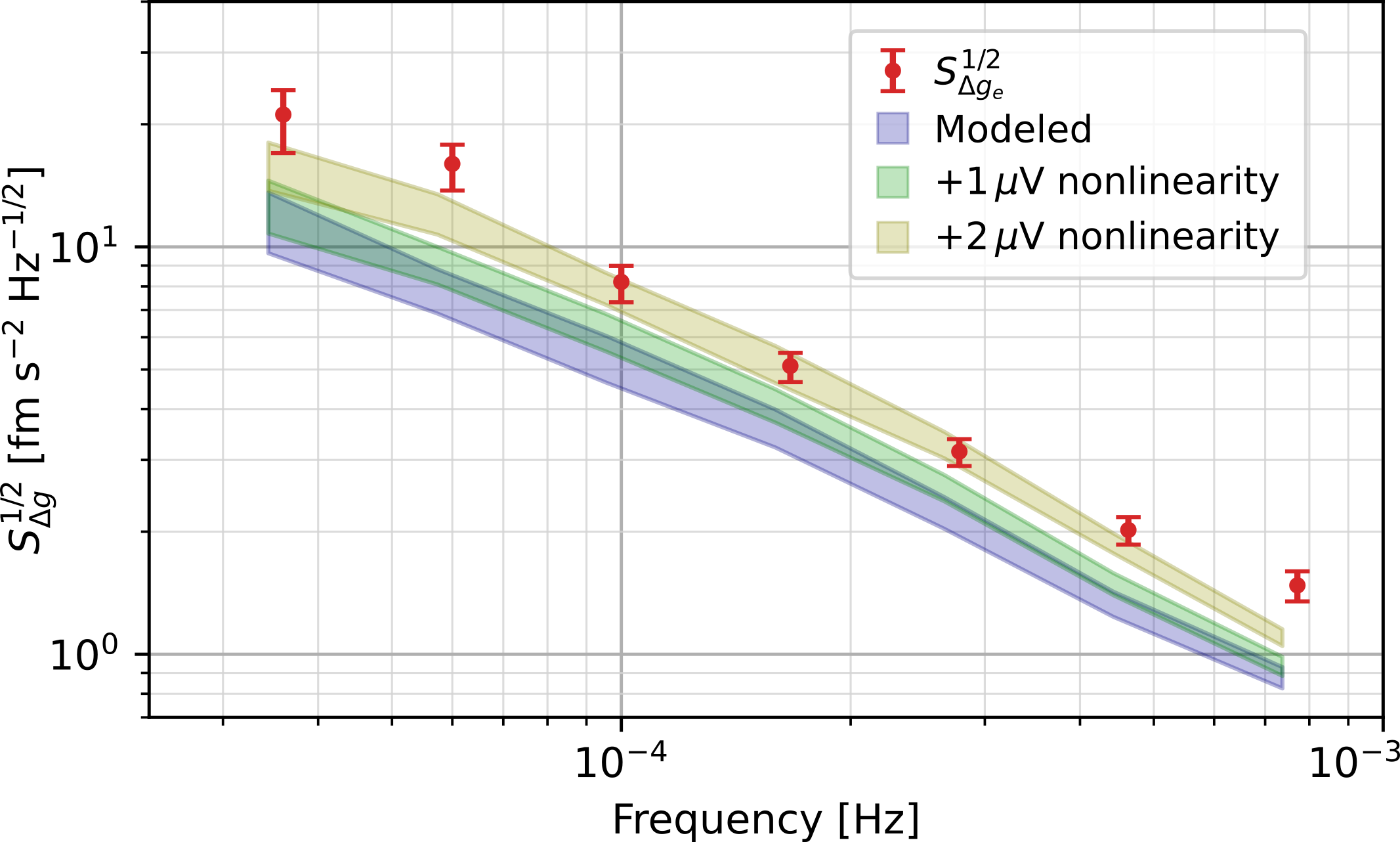
Another mechanism through which voltage disturbances could lead to increased in-band force noise and, at the same time, go undetected in dedicated measurement campaigns, is through down-conversion of high-frequency spurious disturbances. If voltage anomalies should be present at frequencies outside the measurement band, they would down-convert into the band because of the quadratic nature of the electrostatic force. In addition, due to the lack of significant associated torque, the voltage anomaly should have involved one or more pairs of electrodes facing the same face of the same TM.

To fix the amplitude scale of such a disturbance, the force due to the voltage $V$, when applied to both electrodes in one such pair, exerts a force $\lvert\Delta g\rvert=(1/M)\lvert\partial C_{x}/\partial x\rvert V^{2}\simeq 0.15\,\text{pm\,s}^{-2}\,(V/100\,\text{mV})^{2}$. Thus a line with a mean amplitude of 100 mV, and a noisy relative amplitude fluctuation with ASD $\simeq 5\times 10^{-3}/\sqrt{\text{Hz}}\,(1\,\text{mHz}/f)$ would produce the observed noise. We note that the actuation circuitry connected to the electrodes includes a passive two-stage lowpass filter with a bandpass near 2 kHz, thus this putative high-frequency disturbance would have needed to be accordingly higher at the amplifier outputs for frequencies larger than 2 kHz.

No such line has been detected either during the ground testing of the FEE flight hardware, or during laboratory testing of its various prototypes, but we cannot exclude for instance some damage due to the launch stresses.

IX.3 Unmodeled gravitational noise

We have discussed the gravitational noise due to propellant tank depletion and that due to LTP distortion. We have accounted for the first and estimated that it is unlikely that the second may have caused more than 10% of the unaccounted noise.

Besides those effects, any other mass motion, either because of distortion of solid parts or because of evaporation of volatile fractions, may cause gravitational force noise and may have contributed to excess noise. We discuss here a few possibilities, first for the case of distortion and then for that of evaporation.

The Tungsten balance mass is the most intense source of gravitational field gradient at the TM location. The LTP distortion, already discussed, moves the balance mass, relative to the TM, together with the entire GRS. However, in addition to that, any internal GRS distortion may also have moved the balance mass relative to the TM.

With a gravitational gradient $\simeq\partial g_{x}/\partial x_{s}\simeq 5\times 10^{-7}\,\text{s}^{-2}$, a random jitter $\delta x$ of the balance mass position with ASD $S_{\delta x}^{1/2}\simeq$1.5\text{\,}\mathrm{n}\mathrm{m}\mathrm{/}\sqrt{\text{Hz}}$\,\left($1\text{\,}\mathrm{m}\mathrm{H}\mathrm{z}$/f\right)$, would account for the entire unexplained excess. Such a jitter, if thermally induced, given the construction materials and the geometry of the GRS, would amount to thermal fluctuations with an ASD of $S_{T}^{1/2}\simeq$4\text{\,}\mathrm{m}\mathrm{K}\mathrm{/}\sqrt{\text{Hz}}$\,\left($1\text{\,}\mathrm{m}\mathrm{H}\mathrm{z}$/f\right)$, definitely larger than the measured one [8].

As for non-thermal deformation, an obvious example would be long-term, noisy mechanical secondary creep due to stress release, like that due to the unlock of the TM on orbit. Crudely approximating this creep as a Poisson sequence of steps with root mean square (rms) amplitude $\delta x$, and average relaxation rate $\delta\dot{x}$, one would need $\delta x\delta\dot{x}\simeq$0.2\text{\,}\mathrm{\SIUnitSymbolMicro}\mathrm{m}^{2}\mathrm{/}\mathrm{yr}$$. As realistically $\delta\dot{x}\ll\,$\mathrm{\SIUnitSymbolMicro}\mathrm{m}^{2}\mathrm{/}\mathrm{yr}$$, this would require steps of $0.2\text{\,}\mathrm{\SIUnitSymbolMicro m}$, happening then at a rate of less than 5 per year, very different from the observed time series.

Thermal or non-thermal distortion resulting in the motion of massive components farther away from the TMs may also exert significant forces. Calculations [47] show for instance that the spacecraft alone, without the LTP, exerts a static difference of force on the TM of $\Delta g_{sc}\simeq 5\times 10^{-9}\,$\mathrm{m}\,\mathrm{s}^{-2}$$, very similar to that of a homogeneous square toroid with an inner diameter of one meter, an outer one of two meter, and a mass of $\simeq$300\text{\,}\mathrm{k}\mathrm{g}$$, a crude approximation to the spacecraft shape.

One can calculate that a homogeneous relative distortion $\delta$ of any of the toroid dimensions, causes a variation of differential force $\delta\times\Delta g_{sc}$. It would thus take $\delta$ to be a random process with ASD $S_{\delta}^{1/2}\simeq 1.4\times 10^{-7}\,$\mathrm{Hz}^{-1/2}$\,($1\text{\,}\mathrm{m}\mathrm{H}\mathrm{z}$/f)$ to justify the unexplained noise.

We have no way of assessing if such mechanical distortions of the spacecraft (about $0.1\text{\,}\mathrm{\SIUnitSymbolMicro m}$ root-mean-square variation of the corresponding dimension over 1 day) did take place during operations. A correlation analysis of $\Delta g$ with the solar power hitting the spacecraft gave no significant results. A simulation of thermal induced distortion and of the resulting gravitational noise performed during mission development [47], pointed to one order of magnitude smaller figures. This simulation was done though on a simplified model and was significant only for $f\gtrsim$2\text{\,}\mathrm{m}\mathrm{H}\mathrm{z}$$.

All that said, detailed thermo-mechanical simulations are standard practice in aerospace engineering. In addition, for LPF rather complete tools have been set up to interface the thermo-mechanical model of the system with the gravitational one. We calculate that a thorough dynamical simulation of the LISA spacecraft’s gravitational field should have the accuracy and the sensitivity to keep gravitational noise due to mechanical distortion under control.

Outgassing of volatile fractions from spacecraft has been observed, for instance in the Rosetta mission, to continue years after launch [48]. In particular, after a water desorption-dominated phase lasting 100-200 days, a longer, possibly diffusion-dominated phase was observed, with a very slowly, if at all decaying evaporation rate, at least for the following 500 days.

Given the non-symmetric geometry of the LPF spacecraft, even a spatially homogeneous noisy outgassing would have caused some $\Delta g$ noise. Definitely more so if the outgassing had also some patchy pattern, that would have further reduced the spatial symmetry.

To fix the scale of the effect, we have considered the spacecraft structure, which is made out of sandwich panels of Carbon Fiber Reinforced Plastic (CFRP) with an aluminum honeycomb core. We have considered the case of N outgassing patches of size small enough to approximate sums with integrals, having noisy evaporation rates all with same ASD, incoherently adding up to a total evaporation rate with ASD $S_{\dot{M}}^{1/2}$.

We calculate that $S_{\Delta g}^{1/2}\simeq 0.5\left(\mathcal{G}/L_{0}^{2}\right)S_{\dot{M}}^{1/2}/(2\pi f)$, with $L_{0}=37.6\text{ cm}$ the distance between the centers of the two TMs, and $\mathcal{G}$ the gravitational constant. To match our observation of $S_{\Delta g}^{1/2}\simeq$0.7\text{\,}\mathrm{f}\mathrm{m}\,\mathrm{s}^{-2}\mathrm{/}\sqrt{\text{Hz}}$\,(1\,\text{mHz}/f)$, we need a frequency independent value $S_{\dot{M}}^{1/2}\simeq$0.02\text{\,}\mathrm{m}\mathrm{g}\,\mathrm{s}^{-1}\mathrm{/}\sqrt{\text{Hz}}$$.

Just for the sake of discussion, we note that such a “white” evaporation rate behavior would naturally be obtained if the outgassing on LPF consisted of a Poisson succession, with mean evaporation rate $\langle\dot{M}\rangle$, of discrete outgassing events from any of the patches, with a rms value $\delta m$. This process would indeed give $S_{\dot{M}}^{1/2}=(\delta m\,\langle\dot{M}\,\rangle)^{1/2}$.

Ref. [48] estimates the mass loss of Rosetta in several hundred grams per year. LPF was a lighter satellite, by almost a factor 3, but with more plastic and closer to the sun. Thus a direct projection of the outgassing properties may be rather speculative.

Nevertheless, a crude estimate based on the outgassing properties of LPF materials, gives a lower limit for $\langle\dot{M}\rangle$ at $\langle\dot{M}\rangle\simeq$0.1\text{\,}\mathrm{k}\mathrm{g}\,\mathrm{y}^{-1}$=$3\text{\,}\mathrm{\SIUnitSymbolMicro}\mathrm{g}\,\mathrm{s}^{-1}$$, not far from what one would extrapolate from Rosetta based just on the mass ratio of the two satellites. Using this figure for $\langle\dot{M}\rangle$ in the Poisson noise ASD formula, one gets $\delta m\simeq$0.2\text{\,}\mathrm{m}\mathrm{g}$$ and $\lambda=\langle\dot{M}\rangle/\delta m\simeq$0.01\text{\,}\mathrm{s}^{-1}$$.

To our knowledge, there are no studies on the spatial distribution of outgassing in spacecraft, nor on its dynamics. Thus this crude scenario of noisy outgassing remains rather speculative. We note however that nothing, in the figures above, or in the current knowledge, allows us to rule it out. We conclude that a cautious approach for LISA would be to stay as close as possible to the LPF design in terms of quantity and distribution of materials with significant volatile components.

IX.4 Pressure fluctuation

As said in Sec. V.6, the complex geometry of the TM environment may create quasi-static pressure gradients. Any in-band fluctuation of such gradients would directly translate into an in-band acceleration fluctuation.

To account for the measured excess $S_{\Delta g_{e}}^{1/2}$ of about $0.7\,$\mathrm{f}\mathrm{m}\,\mathrm{s}^{-2}\mathrm{/}\sqrt{\text{Hz}}$\,($1\text{\,}\mathrm{m}\mathrm{H}\mathrm{z}$/f)$, the ASD of these fluctuations should be $S_{\Delta p}^{1/2}\sim 0.6\times 10^{-12}\,$\mathrm{Pa}\mathrm{/}\sqrt{\text{Hz}}$\,($1\text{\,}\mathrm{m}\mathrm{H}\mathrm{z}$/f)$.

We note that the process at the basis of this hypothetical fluctuating pressure should necessarily be different from that generating the static gradient discussed in Sec. V.6. Indeed, (see Sec. IV) the latter steadily decreased during the mission, following the general decay of the pressure, whereas the former (Sec. V.2) did not.

Hence, if the process responsible for the $1/f$ noise has been due to the outgassing of some species for the TM environment, it must have been substantially stable over the entire mission and independent of the outgassing rate of the main fraction. This observations parallels that on the possible outgassing origin of force glitches in LPF [20] that also had properties that have been stable over the course of the entire mission.

It does not require much outgassing to produce the $1/f$ noise. If for instance such hypothetical gas phase were hydrogen diffusing out of the various elements of the TM environment, and if the noisy outgassing took place as the series of undetectable glitches discussed in Sec. VII.2 and in the App. G, it would only take a mean outgassing rate of $\simeq 6\text{ pg/d}$, that is some 3 ng of total emission over the course of the entire mission, to explain the noise. We have no specific piece of experimental evidence to support this hypothesis, neither we could trace any relevant study on pressure fluctuations in vacuum systems. Neither we have, however, any evidence proving the model false or unlikely, neither from our own experiments nor from the literature. It is also unlikely that we could devise a laboratory experiment able to detect such tiny pressure fluctuations.

For this reason, we conclude again that the LISA GRS outgassing environment should be kept as close as possible to that of LPF, to retire the risk of unwanted large pressure gradient fluctuations.

IX.5 High frequency magnetic field noise

In addition to low-frequency effects, discussed in Sec. VIII, magnetic fields at high frequency may induce eddy currents within the test masses, and then exert Lorentz forces on them [49]. The effect is thus quadratic and would convert the low frequency amplitude fluctuations of a high frequency magnetic spectral line into a corresponding low frequency force.

To give a scale of the effect, a recent finite-element electromagnetic calculation by the LISA project [50], has shown that the effect of a dipole of $1\text{\,}\mathrm{m}\mathrm{A}\,\mathrm{m}^{2}$ located at a distance $d=$20\text{\,}\mathrm{c}\mathrm{m}$$ from the test mass and oscillating at the frequency of 100 Hz, would cause a force of $\Delta g\simeq$4\text{\,}\mathrm{f}\mathrm{m}\mathrm{/}\mathrm{s}^{2}$$. The effect reaches its peak at $100\text{\,}\mathrm{Hz}$, while at lower frequency the induced current decreases, and above that, the screening effect of the metallic electrode housing attenuates the oscillating field. The effect of a dipole source decreases with $d^{-7}$, so that at the closest distances of about $0.4\text{\,}\mathrm{m}$ between the test mass and any active device on the LPF spacecraft the effect might be $\sim 100$ times smaller.

The spacecraft prime contractor, during LPF development, performed a test campaign on ground against audio frequency magnetic lines [51]. A few, barely significant lines have been identified, with peak amplitudes $\ll$1\text{\,}\mathrm{nT}$$ at the position of the test masses. In the point dipole model at a distance of $d\simeq$0.4\text{\,}\mathrm{m}$$, a $1\,\text{nT}$ line would be generated by a dipole of $\simeq$0.3\text{\,}\mathrm{m}\mathrm{A}\,\mathrm{m}^{2}$$ at most, and would exert a static force $\Delta g\simeq$4\text{\times}{10}^{-3}\text{\,}\mathrm{f}\mathrm{m}\,\mathrm{s}^{-2}$$. To reproduce the observed excess noise with a noisy amplitude modulation of one of these lines $1\text{\,}\mathrm{nT}$, one would need a relative amplitude modulation with ASD $\simeq 2.5\times 10^{2}\text{\,Hz}^{-1/2}\left(1\,\text{mHz}/f\right)$.

One can calculate that the rms fluctuation of a process $x$ with ASD given by $S_{x}=S_{0}^{1/2}(f_{0}/f)$, over a data stretch of duration $T$, is $\langle x_{\text{rms}}\rangle=S_{0}^{1/2}\pi f_{0}\sqrt{T/3}$. With $S_{0}^{1/2}\simeq 2.5\times 10^{2}\text{\,Hz}^{-1/2}$, it would take about 5 s to make the relative rms fluctuation of the line amplitude 100%. Such a large fluctuation would have been noticed during testing.

The required amplitude fluctuation for such lines would become smaller in the presence of more than one line. However consider that 1 nT is a real conservative upper limit for the observed lines, and that the effect is quadratic in the amplitude of the lines, so that the combined effect of many lines would be dominated by the few brightest among them.

Despite these considerations, that would rule out this source of noise, it must be stressed that unfortunately we had no magnetometer on board sensitive to the audio band. Thus, as the operating conditions may have been different from those during testing, we cannot exclude that additional, more intense, amplitude-modulated lines had been generated once on orbit.

For instance, a single line generated by a dipole of $\simeq$2\text{\,}\mathrm{m}\mathrm{A}\,\mathrm{m}^{2}$$ located at a distance $d=$20\text{\,}\mathrm{c}\mathrm{m}$$ from the test mass, with a more reasonable relative amplitude fluctuation ASD $\simeq$0.2\text{\,}\mathrm{Hz}^{-1/2}$\left(1\,\text{mHz}/f\right)$, would explain the excess noise. This is a relatively large magnetic dipole, for instance 32 mA in a fully uncompensated square loop of 25 cm size, of the existence of which we are not aware. Nevertheless we certainly recommend that in LISA thorough testing is performed on ground, and that on-board diagnostic magnetometers with sensitivity up to, at least, $1\text{\,}\mathrm{kHz}$ are seriously considered.

X Concluding remarks

LISA Pathfinder reached an acceleration noise performance achieving the LISA requirements with margin, and better than both its requirements and what had been estimated before launch [49].
This last achievement was mostly allowed by two facts:

• A much better self-gravity cancellation than what had been very cautiously estimated on ground. This in turn allowed using much less electrostatic force authority than predicted [2], and suppressing accordingly the actuation noise.

• The achievement, over the course of the mission, of a lower base pressure, and thus a lower Brownian noise, than had been assumed in pre-launch estimates [49].

Both these facts revealed the existence of an excess noise above the Brownian noise level, with a $1/f^{2}$ PSD.
Based on this starting framework, in this paper we have:

• shown that the Brownian noise evolved in agreement with the outgassing of a single gaseous species diffusing out of the immediate, complex surroundings of the TM, where such outgassing also maintains a quasi-static pressure gradient across the TM;

• shown that the temperature stability of the system was good enough that temperature fluctuation played a significant role in the acceleration noise only at the lowest analyzed frequency $18\text{\,}\mathrm{\SIUnitSymbolMicro Hz}$, well below the LISA lower frequency of $0.1\text{\,}\mathrm{mHz}$;

• shown that the intrinsic stability of the $1/f^{2}$ excess PSD (referred to in the article as $1/f$ excess for ASD) was $\pm 20\%$ in amplitude over more than 16 months, with the residual fluctuations being independent of any traceable change in the operational conditions that were needed to run the mission;

• analyzed all sources of noise for which we had a verified model, either from correlation analysis or from dedicated experiments, and concluded that these sources account for a fraction $0.46\pm 0.09$ of the total power of the excess;

• finally, we have discussed all possible explanations we could trace for the unaccounted part of the excess, with patch potentials, actuation electronics nonlinearity, audio frequency magnetic fields, and pressure fluctuations as the prominent ones, and identified possible measures to keep them under full control during the implementation of LISA.

Appendix

The following appendices contain some rather important information, tables, and calculations.
In App. A, we give details about the analyzed noise runs.
In App. B, we describe our spectral analysis tools and decorrelation methods.
In App. C, we list the frequencies used in PSD estimation.
In App. D, we provide the ASD of $\Delta g(t)$ for all analyzed noise runs.
In App. E, we present the calculations for instrument distortion analysis and the drift evaluation procedure.
In App. F, we present the calculations for in-band noise of instrument distortion and thermal effects.
In App. G, we study whether a Poisson flow of low-amplitude glitches could produce noise with the observed properties.

Appendix A Experimental configurations for the 13 runs

There were minor differences in the operating conditions of the 13 runs of Table 1. We describe them in the following and summarize the different configurations in Table 2.

Run	Propellant	Thruster	Actuation	TM	Voltage	Heaters	ST7
	tank	branch	authority	alignment	compensation	configuration	state
1	2	A	URLA	1	1	1	OFF
2	2	A	UURLA	1	1	1	OFF
3	2	A	UURLA	1	2	1	OFF
4	3	A	UURLA	2	3	1	OFF
5	3	A	UURLA	3	3	2	DIAG
6	1	A	UURLA	3	3	2	DIAG
7	3	B	UURLA	3	3	2	DIAG
8	1	B	UURLA	3	3	3	DIAG
9	1	B	UURLA	3	4	4	OFF
10	1	B	UURLA	3	4	5	OFF
11	3	A	UURLA	3	4	6	OFF
12	3	A	UURLA	3	4	1	OFF
13	3	A	UURLA	3	4	1	OFF

TABLE 2: Experimental configuration for the 12 different runs of Table 1. The meaning of the numeric labels is explained in the text.

• Thruster propellant was stored in three different tanks. The gravitational signal from the depletion of these tanks was different, due to the different positions. In Table 2, we name these three tanks as 1, 2, and 3.

• For redundancy reasons, LPF carried two independent branches of micro-thrusters [13]. In Table 2, we call them A and B.

• The electrostatic controllers needed a setting for the maximum force/torque authority they could deliver within a linear regime [19]. These settings determine the zero-actuation voltages commanded to the various electrodes. The settings were identical for all the considered runs except for the first one. Values are reported in Table 3.

  	URLA	UURLA
  $F_{x,1}$ [pN]	0	0
  $F_{x,2}$ [pN]	50	50
  $N_{x,1}$ [pN m]	16.37	4
  $N_{x,2}$ [pN m]	16.37	4
  $F_{y,1}$ [pN]	3670	1000
  $F_{y,2}$ [pN]	3670	1000
  $N_{y,1}$ [pN m]	13.32	4
  $N_{y,2}$ [pN m]	13.32	4
  $F_{z,1}$ [pN]	5820	500
  $F_{z,2}$ [pN]	5820	500
  $N_{z,1}$ [pN m]	1.5	1.5
  $N_{z,2}$ [pN m]	1	1

  TABLE 3: Maximum actuation authorities, $F_{a,i}$ and $N_{a,i}$, respectively the maximum force and the maximum torque applicable on TM$i$ along axis $a$.

• In the attempt to reduce cross-talk between the differential interferometer readout and the motion of the remaining TM degrees of freedom [16], we performed three different adjustments of the zero set points of all control loops. The most relevant ones were those for the angular orientations of the TM along $z$ and $y$. The three set points, named 1, 2, and 3, are listed in Table 4.

  Angle	Set point	Set point	Set point
  $($\mathrm{\SIUnitSymbolMicro rad}$)$	1	2	3
  $\phi_{1}$	-59.25	-56.32	-61.2
  $\phi_{2}$	-21.35	-33.01	-9.7
  $\eta_{1}$	-3.5	-2.14	-4.9
  $\eta_{2}$	3.5	10.3	-3.3

  TABLE 4: The three different set points for the angular orientations of the TMs along $z$ ($\phi$) and $y$ ($\eta$), used during the noise runs. The index indicates which TM each angle refers to. Angles are relative to a reference frame defined by the OMS.

• Random TM charging due to cosmic rays couples to DC voltage differences between the TM and the surrounding metal surfaces to produce random force and torque [22]. This noise may be suppressed by purposely applying some DC voltages to the various electrodes, in order to compensate the parasitic ones that are found on metal surfaces because of work function differences [22]. In particular, the force along $x$ and the torque along $\phi$, may be compensated by a proper combination of voltages on the electrodes facing the $x$-faces of the TMs. These compensation voltages may be described by just voltage parameters $\Delta_{x}$ and $\Delta_{\phi}$ as explained in [22]. In the course of the mission we have made some adjustments of these parameters for both TMs. The various configurations are listed in Table 5.

  Voltage	Setting	Setting	Setting	Setting
  (mV)	1	2	3	4
  $\Delta_{x,1}$	0	+24	+12	+24
  $\Delta_{x,2}$	0	0	0	0
  $\Delta_{\phi,1}$	0	0	0	+32
  $\Delta_{\phi,2}$	0	0	0	-116

  TABLE 5: Compensation voltages for the 4 adopted settings. The index indicates the TM.

• While the noise runs in Table 1 were all performed by using the satellite cold gas thrusters for drag-free control [13], LPF also carried a set of alternative thrusters based on colloidal propellant technology, in the framework of NASA ST7 mission [52]. These thrusters were used intermittently, leaving them, for purpose of diagnostics, in some activated state even when not in use, in the two epochs from June 27, 2016 to December 7, 2016, and from March 18, 2017 to April 29, 2017. In Table 2 we indicate such state as DIAG, while the completely off state is indicated with OFF.

Appendix B Spectral estimation methods

B.1 Periodograms and their spectral properties

We use, for the elementary periodogram $X(k)$ of the $N$-sample series $x[n]$, sampled with sampling time $T$, the standard definition:

$$X(k)=\sqrt{\frac{T}{N}}\sum_{n=0}^{N-1}x[n]w[n]\,e^{-2\pi ikn/N},$$ (18)

where $w[n]$ are the coefficients of a Blackman-Harris spectral window, which gives good side-lobe suppression [53].

Following the Welch method [54], we section our data series in as many 50% overlapping data stretches of length $N$ as they fit into the length of the data series, and define the average, one-sided experimental PSD at frequency $f$:

$$\Pi\left(f=\frac{k}{NT}\right)=\frac{2}{M}\sum_{l=1}^{M}X_{(l)}(k)X_{(l)}^{*}(k),$$ (19)

where the index $l$ runs over the $M$ data stretches, and $k$ is the frequency index.

For multiple, synchronously measured data series $x_{i}[n]$, with $1\leq i\leq p$, Eq. (19) generalizes to the (one-sided) experimental cross-spectral density (CPSD) matrix $\bm{\Pi}$, with elements:

$$\Pi_{ij}\left(f=\frac{k}{NT}\right)=\frac{2}{M}\sum_{l=1}^{M}X_{i,(l)}(k)X_{j,(l)}^{*}(k),$$ (20)

a complex and Hermitian matrix. It is also positive-definite if $M\geq p$. Our founding point is that, if the $x_{i}(t)$ are Gaussian, zero-mean stationary stochastic processes, with a theoretical cross-spectral density matrix $\bm{\Sigma}$, then the matrix $\bm{W}$, whose elements are $W_{ij}=M\Pi_{ij}$, is distributed like a complex Wishart distribution [55, 56]:

$$p\left(\bm{W}\big{|}\bm{\Sigma}\right)=\frac{\left|\bm{W}\right|^{M-p}}{\widetilde{\Gamma}_{p}(M)\left|\bm{\Sigma}\right|^{M}}\ \mathrm{etr}\left[-\bm{\Sigma}^{-1}\bm{W}\right]$$ (21)

Where $\left|\cdot\right|$ is the determinant, $\mathrm{etr}$ the exponential trace $\mathrm{etr}(\cdot)=\exp\left(\mathrm{tr}\left(\cdot\right)\right)$ and $\widetilde{\Gamma}_{p}(M)$ is the multivariate complex Gamma function, defined by

$$\widetilde{\Gamma}_{p}(M)=\pi^{\frac{1}{2}p(p-1)}\prod_{i=1}^{p}\Gamma(M-i+1)$$

We denote this distribution as $\mathcal{CW}(\bm{\Sigma},M)$, and indicate that $\bm{W}$ follows this distribution as $\bm{W}\sim\mathcal{CW}(\bm{\Sigma},M)$.

Note that in Eq. (21) it is required that $M\geq p$, otherwise the matrix $\bm{W}$ is singular. This distribution is the basis of our spectral analysis method.

B.2 PSD estimation

For $p=1$, $\mathcal{CW}(\bm{\Sigma},M)=\mathcal{CW}(S_{x},M)=\Gamma(M,M/S_{x})$, with $\Gamma(\alpha,\theta)$ the gamma distribution with shape parameter $\alpha$ and scale parameter $\theta$, and with $S_{x}$ the theoretical PSD of the sole series $x(t)$.

This distribution can be used, along with a proper prior, to build the Bayesian posterior for $S_{x}$. According to standard, physically sound practice, we take an uninformative flat prior in the logarithm of $S$, which is a prior proportional to $1/S$. For $p=1$ this also coincides with the Jeffreys, re-parametrization independent prior [26].

Such choice gives a posterior for $S$ that is distributed as an inverse-Gamma distribution, with shape parameter $M$ and scale parameter $M\Pi$:

$$p(S|\Pi,M)\sim\text{inv}\Gamma\left(M,M\Pi\right)$$ (22)

The expected value of this posterior, $\langle S\rangle=M\Pi/(M-1)$, is slightly biased and diverges for $M\to 1$. However, the posterior probability density function remains well-behaved even in the limit case; we have checked, by a simple numerical simulation, that for all values of $M$ and for Gaussian data, the theoretical value lies in the $p$-credible interval with probability $p$.

Based on this posterior distribution, we compute the equally-tailed $p$-credible interval from the $(1\pm p)/2$ quantiles of the distribution. Unless otherwise specified, error bars in our plots correspond to $p=68.3\%$, as for the $\pm 1\sigma$ interval in a normal distribution. The dots in those same plots represent the median of the distribution, which remains well behaved also for $M=1$, and has a smaller bias than the mean.

B.3 Decorrelation methods

Here we describe the method used to assess the contribution to $S_{\Delta g}$ of the disturbances for which we have a synchronously measured time series. As said in the main text, we had to face two separate cases: one in which the susceptibilities $\alpha_{i}$ in Eq. (14) are reasonably known, but the time series of the disturbance carries some significant readout noise; in the second case, on the contrary, the susceptibilities are unknown, except for some rather loose order of magnitude estimate, but the readout noise can be safely assumed to be negligible. These two cases are separately treated in the following.

B.3.1 Decorrelation of noisy series with known susceptibilities

This is the case when we have a relatively narrow posterior distribution $f(\alpha_{i})$ for the susceptibility $\alpha_{i}$, but $S_{n_{i}}$ may be large, actually may even dominate $S_{z_{i},z_{i}}$ in Eq. (15), and refers to the joint analysis of fluctuations of the average temperature and of LTP distortion in Sec. VIII.2.1, and to that of the tank depletion gravitational signal in Sec. VIII.2.2.

Though the two cases differ substantially, they both share the step of estimating the Bayesian posterior for $\bm{\Sigma}$, the theoretical CPSD.

To that purpose, our starting point is again the distribution in Eq. (21) that can be directly used to estimate the Bayesian posterior for $\bm{\Sigma}$, or its inverse $\bm{Q}=\bm{\Sigma}^{-1}$, from the observation of $\bm{W}$, once a prior distribution for either $\bm{\Sigma}$ or $\bm{Q}$ has been assumed.

Natural, non-informative choices are either a uniform prior on all elements of $\bm{Q}$, or the Jeffreys prior [26], which, for a $p\times p$ dimensional $\bm{Q}$ matrix, is $\propto\lvert\bm{Q}\rvert^{-p}$ [57, 58]. For the uniform prior, the posterior is $\bm{Q}\sim\mathcal{CW}(\bm{W}^{-1},M+p)$, while for the Jeffreys prior $\bm{Q}\sim\mathcal{CW}(\bm{W}^{-1},M)$

Both choices have limitations. Of those of the uniform prior when $p=1$ we have discussed in App. B.2. On the other hand, the Jeffreys prior is affected by bias, and by a significant inconsistency when $p>1$.

The bias consists of the fact that while the mean value of $\bm{Q}$ is unbiased, the mean value of $\bm{\Sigma}$ is equal to $\bm{\Pi}M/(M-p)$. Thus the bias depends on $p$ and may become large at low values of $M$.

The inconsistency stays in the fact that, when $p>1$, the marginal posterior of any of the diagonal elements of $\bm{\Sigma}$, is not the same as the posterior in Eq. (22), which one would calculate from the Jeffreys prior with $p=1$.

The bias can be reduced and made independent of $p$, and the inconsistency solved, if one takes the “intermediate” prior $\propto\lvert\bm{Q}\rvert^{-1}$, that still coincides with the logarithmic prior for the case $p=1$.

Note that, also with this choice, $\bm{Q}$ is Wishart distributed, $\bm{Q}\sim\mathcal{CW}(\bm{W}^{-1},M+p-1)$, which guarantees, without imposing any further prior constraint, that $\bm{Q}$ and its inverse are positive definite matrices, a fundamental constraint for CPSD. We use this posterior to estimate both the entire matrix, in the case of temperature/LTP distortion, or its $S_{z_{i},\Delta g}(f)$ elements, in the case of the tank depletion noise.

As we have a closed formula, we generate random samples both from such posterior for $\bm{Q}$ and from the posterior for the $\alpha_{i}$, and calculate then the samples of the quantities needed in the two cases, as discussed in their relative sections.

B.3.2 Decorrelation of disturbances with unknown susceptibilities and negligible readout noise

In the case of unknown susceptibilities and negligible readout noise, we evaluate $S_{\Delta g_{0}}(f)$, and the susceptibilities assuming the physically realistic model of real, and frequency-independent susceptibilities.

The starting point is that one can transform the distribution in Eq. (21) to separate its dependence on $S_{\Delta g_{0}}$, and the $\alpha_{i}$, from that on the CPSD of the disturbances $S_{y_{i},y_{j}}$.

To do that consider that Eq. (14) defines a linear transformation $\Delta g_{0}\to\Delta g,y_{i}\to y_{i}$ whose matrix is

$$\bm{U}=\left(\begin{matrix}1&\alpha_{1}&\dots&\alpha_{r}\\ 0&1&\dots&0\\ \vdots&&\ddots&\vdots\\ 0&\dots&\dots&1\end{matrix}\right)$$ (23)

Note that $\lvert\bm{U}\rvert=1$, and that the inverse of $\bm{U}$ is obtained with the transformation $\alpha_{i}\to-\alpha_{i}$.

As $\Delta g_{0}$ is independent of the $y_{i}$, before the transformation, the processes have a CPSD matrix with block representation

$$\bm{\Sigma}^{\prime}=\left(\begin{matrix}S_{\Delta g_{0}}&0\\ 0&\bm{\Sigma}_{yy}\end{matrix}\right)$$ (24)

where $\bm{\Sigma}_{yy}$ is the $r\times r$ CPSD of the $y_{i}$. Note that

$$\bm{\Sigma}^{\prime-1}=\left(\begin{matrix}1/S_{\Delta g_{0}}&0\\ 0&\bm{\Sigma}_{yy}^{-1}\end{matrix}\right),$$ (25)

and that $\bm{\Sigma}=\bm{U}\bm{\Sigma}^{\prime}\bm{U}^{T}$, with $\bm{U}^{T}$ the transpose of $\bm{U}$, so that $\lvert\bm{\Sigma}\rvert=\lvert\bm{\Sigma}^{\prime}\rvert=S_{\Delta g_{0}}\lvert\bm{\Sigma}_{yy}\rvert$.

Furthermore, in Eq. (21) one can calculate that $\mathrm{etr}\left[-\bm{\Sigma}^{-1}\bm{W}\right]=\mathrm{etr}\left[-(\bm{U}^{T})^{-1}\bm{\Sigma}^{\prime-1}\bm{U}^{-1}\bm{W}\right]=\mathrm{etr}\left[-\bm{\Sigma}^{\prime-1}{\bm{W}}^{\prime}\right]$, having defined ${\bm{W}}^{\prime}=\bm{U}^{-1}\bm{W}(\bm{U}^{T})^{-1}$.

We need one more step to get our separation. $\bm{W}$ and ${\bm{W}}^{\prime}$ have block representation

$$\bm{W}=\left(\begin{matrix}W_{1,1}&\bm{W}_{1,y}\\ \bm{W}_{1,y}^{\dagger}&\bm{W}_{yy}\end{matrix}\right)\qquad{\bm{W}}^{\prime}=\left(\begin{matrix}{W}^{\prime}_{1,1}&{\bm{W}^{\prime}}_{1,y}\\ {\bm{W}^{\prime}}_{1,y}^{\dagger}&\bm{W}_{yy}\end{matrix}\right)$$ (26)

where one can calculate that

$$\begin{split}&{W}^{\prime}_{1,1}=W_{1,1}-2\bm{\alpha}\cdot\text{Re}\bm{W}_{1,y}+\bm{\alpha}\cdot\text{Re}\bm{W}_{yy}\cdot\bm{\alpha},\end{split}$$ (27)

with $\alpha$ the r-vector the components of which are the susceptibilities.

The consequence of Eqs. 25, 26, and 27 is that

$$\begin{split}&\mathrm{etr}\left[-\bm{\Sigma}^{-1}\bm{W}\right]=\mathrm{etr}\left[-\bm{\Sigma}^{\prime-1}\tilde{\bm{W}}\right]=\\ &=e^{-\frac{{W}^{\prime}_{1,1}}{S_{\Delta g_{0}}}-\text{tr}\left[\bm{\Sigma}_{yy}^{-1}\bm{W}_{yy}\right]}=\\ &=e^{-\frac{W_{1,1}-2\bm{\alpha}\cdot\text{Re}\bm{W}_{1,y}+\bm{\alpha}\cdot\text{Re}\bm{W}_{yy}\cdot\bm{\alpha}}{S_{\Delta g_{0}}}-\text{tr}\left[\bm{\Sigma}_{yy}^{-1}\bm{W}_{yy}\right]}.\end{split}$$ (28)

Putting all together, the distribution of $\bm{W}$, conditional on the susceptibilities, the PSD of the residual noise, and the CPSD of the disturbances, becomes then:

$$p\left(\bm{W}\big{|}\alpha_{i},S_{\Delta g_{0}},\bm{\Sigma}_{yy}\right)=\frac{\left|\bm{W}\right|^{M-p}}{\widetilde{\Gamma}_{p}(M)}\times$$ (29)

$$\times\frac{1}{S_{\Delta g_{0}}^{M}}e^{-\frac{W_{1,1}-2\bm{\alpha}\cdot\text{Re}\bm{W}_{1,y}+\bm{\alpha}\cdot\text{Re}\bm{W}_{yy}\cdot\bm{\alpha}}{S_{\Delta g_{0}}}}\times$$

$$\times\frac{1}{\left|\bm{\Sigma}_{yy}\right|^{M}}\mathrm{etr}\left[-\bm{\Sigma}_{yy}^{-1}\bm{W}_{yy}\right]$$

The distribution in Eq. (29) can be used to build a joint posterior for $S_{\Delta g_{0}}^{-1}$ and the $\alpha$’s, and an independent posterior for $\bm{\Sigma}_{yy}$.

Treating the data at the different frequencies as independent, and assuming that $S_{\Delta g_{0}}$ and $\bm{\Sigma}_{yy}$ depend on the frequency, while the $\alpha$’s do not, the joint likelihood for the Bayesian inference of $S_{\Delta g_{0}}$ and $\alpha_{i}$ becomes:

$$\begin{split}&p(\alpha_{i},S_{\Delta g_{0}}(f_{1}),S_{\Delta g_{0}}(f_{2}),\dots|\bm{W})\propto\\ &\propto\prod_{k}\frac{\widetilde{p}(S_{\Delta g_{0}}(f_{k}))}{S_{\Delta g_{0}}(f_{k})^{M(f_{k})}}e^{-\sum_{k}\frac{W_{1,1}(f_{k})}{S_{\Delta g_{0}}(f_{k})}}\times\\ &\times e^{2\bm{\alpha}\cdot\sum_{k}\frac{\text{Re}\bm{W}_{1,y}(f_{k})}{S_{\Delta g_{0}}(f_{k})}-\bm{\alpha}\cdot\left(\sum_{k}\frac{\text{Re}\bm{W}_{yy}(f_{k})}{S_{\Delta g_{0}}(f_{k})}\right)\cdot\bm{\alpha}},\end{split}$$ (30)

having taken a flat prior for the $\alpha$’s, and the prior $\widetilde{p}(S_{\Delta g_{0}}(f_{k}))$ for $S_{\Delta g_{0}}(f_{k})$. As for this one, to take into account the presence of the Brownian noise, we split it as $S_{\Delta g_{0}}(f_{k})\to S_{\Delta g_{0}}(f_{k})+S_{\text{Brown}}$, and we take a uniform prior for the logarithms of $S_{\Delta g_{0}}(f_{k})$. For $S_{\text{Brown}}$ we use as prior the posterior obtained for its Bayesian estimate (see Sec. III). At frequencies low enough that the Brownian noise is negligible, which is where the excess is best measured, this is fully equivalent to taking the Jeffreys prior for $S_{\Delta g_{0}}(f_{k})^{-1}$, which is indeed a uniform prior on its logarithm.

To estimate the posterior of the parameters, we employ a parallel-tempering Monte Carlo Markov chain algorithm (PT-MCMC [59]). We always find smooth distributions, no bi-modalities and no strong cross-correlation among parameters. To implement the prior, the MCMC algorithm explores the parameter space of the susceptibilities, and of the logarithms of $S_{\Delta g_{0}}(f_{k})$ and of $S_{\text{Brown}}$.

As for $\bm{\Sigma}_{yy}$, Eq. (29) shows that, using the intermediate prior, $\bm{\Sigma}_{yy}^{-1}(f_{i})\sim\mathcal{CW}(\bm{W}_{yy}^{-1}(f_{i}),M(f_{i})+r-1)$. Thus the evaluation of the statistical properties of the posterior can be obtained numerically from the relative Wishart distribution.

Once the posteriors for $S_{\Delta g_{0}}(f_{k})$, $S_{\text{Brown}}$, $\alpha_{i}$, and possibly for $\bm{\Sigma}_{yy}$, have been obtained, one can calculate the posterior for $S_{c}=\sum_{i,j}\alpha_{i}\alpha_{j}S_{y_{i},y_{j}}=\sum_{i,j}\alpha_{i}\alpha_{j}\left(\Sigma_{yy}\right)_{i,j}$. However, for small values of $S_{c}/S_{\Delta g_{0}}$, the statistics of such a posterior is biased toward high values, with the bias increasing with $r$. This is due to the positive definite quadratic nature of $S_{c}$, which gets rapidly dominated by susceptibility fluctuations.

To deal with this problem we have resorted to calibrating the bias via simulations. Our simulation consists of the following steps:

• We extract a sample of $\bm{\Sigma}_{yy}(f)$ from its calculated posterior, and form a corresponding sample for $\bm{\Sigma}(f)$ assuming $S_{\Delta g_{0}}=0$.

• We generate a random vector of susceptibilities $\alpha_{i}$ from a normal distribution with zero mean, and standard deviation adjusted such that, at some preferred frequency, $S_{c}\simeq\rho S_{\Delta g_{e}}$, with $\rho$ a desired value of the noise power fraction.

• From the susceptibility vector we form the matrix $\bm{U}$ of Eq. (23), and with it we form the sample of the (provisional) matrix $\bm{\Sigma}(f)=\bm{U}\cdot\bm{\Sigma}^{\prime}(f)\cdot\bm{U}^{T}$. This matrix has $\Sigma_{1,1}=S_{\Delta g}(f)=S_{c}(f)$, a number we store as we need for our calibration procedure.

• We then form the final value of the matrix $\bm{\Sigma}$ by substituting the value of $\Sigma_{1,1}$ above, with a random sample extracted from the posterior distribution of $S_{\Delta g}(f)$ (see Eq. (22)). This our theoretical CPSD matrix, which has a value of $S_{c}(f)$, coherent with its elements $\Sigma_{1,j}(f)$, a value for $S_{\Delta g}=S_{\Delta g_{0}}(f)+S_{c}$ coherent with its posterior, and a value of $\bm{\Sigma}_{yy}(f)$ also coherent with its posterior.

• From the matrix $\bm{\Sigma}(f)$ above we generate a random sample of the simulated $\bm{W}$ matrix, using the Wishart distribution in Eq. (21). On each of these simulated samples of $\bm{W}$ we perform our entire Bayesian procedure thus getting, among others, a posterior for $S_{c}(f)$

We repeat the procedure 100 times for different values of the power fraction $\rho$ and we get then, at each value of $\rho$ and at each of the considered frequencies, a distribution of the ‘true’ values of $S_{c,t}(f)$ and a global distribution of the estimated values $S_{c,e}(f)$ for the same quantity (see Fig. 24). We use mean and standard deviations of these distributions, to do a linear, weighted least square fit $S_{c,t}(f)=AS_{e,t}(f)+B$, that we use to correct the observed data. The procedure gives a result close to what one would obtain by just subtracting, from the estimated value of $S_{c}(f)$, the median from the simulation for $\rho=0$. Indeed in some cases, to avoid repeating time-consuming simulations at different values of $\rho$, we adopted this second method.

FIG. 24: $\pm 1\sigma$ intervals for the distributions of the ‘true’ (Tr.) values of $S_{c}(f)$ and for their global estimated posteriors (Est.) over 100 simulations for each case. The power fraction $\rho$ is an approximation of the average at the three highest frequencies. In particular $\rho=0$ is in reality calculated at $\rho\simeq 4\times 10^{-6}$. Data are plotted for clarity at slightly shifted frequency coordinates, but have all been calculated at one of the frequencies $f_{i}$ with $4\leq i\leq 8$.

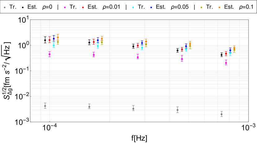
With simulations, we have also checked that the method is unbiased for the estimate of both $S_{\Delta g_{0}}$ and the susceptibilities.

As a final note, the case of the evaluation of the effect of the temperature on the first bin involves just one frequency and one disturbance. In such case the likelihood in Eq. (30) can be integrated analytically, to give a marginal probability density for $S_{\Delta g,0}\sim\text{inv}\Gamma\left(M-1,M/(\bm{\Pi}^{-1})_{1,1}\right)$, for the general case of a complex $\alpha$, and $S_{\Delta g,0}\sim\text{inv}\Gamma\left(M-1/2,M/(\text{Re}\bm{\Pi}^{-1})_{1,1}\right)$ if alpha is real. We have used these formulas to evaluate the effect of the temperature.

Appendix C Choice of quasi-independent frequencies

As presented in [1, Supp.mat.], we evaluate the CPSD at log-spaced frequencies, such that the correlation among adjacent frequencies is kept below 5%. The number of averaged periodograms $M$ varies with frequency, so that the variance is optimally reduced as more periodograms are available. However, $M$ is the same for the first and second frequencies: even though this induces a slightly higher correlation, it allows to analyze the lowest frequency $18\text{\,}\mathrm{\SIUnitSymbolMicro Hz}$. Frequencies are chosen so that the lowest bins always have a fair amount of periodograms, and the fourth one ($0.1\text{\,}\mathrm{mHz}$) is the lower bound of the official LISA frequency band. The frequencies are listed in Table 6.

TABLE 6: List of frequencies used for spectral estimation.

Appendix D ASD of $\Delta g(t)$ for all runs

The following figures, 25 and 26, show the ASD for all runs of Table 1, except for run 10 which is shown in Fig. 2.

FIG. 25: PSD of $\Delta g(t)$ for runs from 1 to 6. The meaning of all symbols is the same as in Fig. 2.

FIG. 26: PSD of $\Delta g(t)$ for runs from 7 to 13, except for run 10 which has already been shown in Fig. 2. The meaning of all symbols is the same as in Fig. 2.

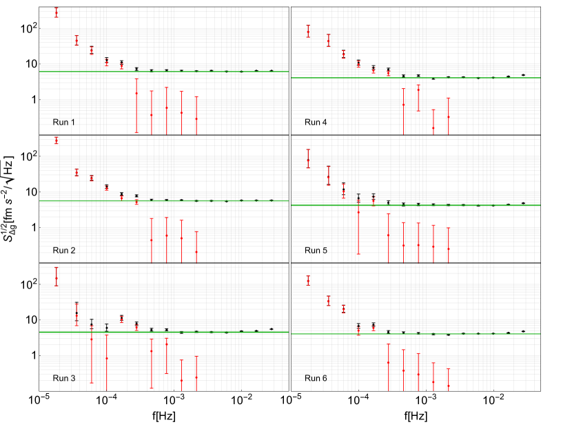
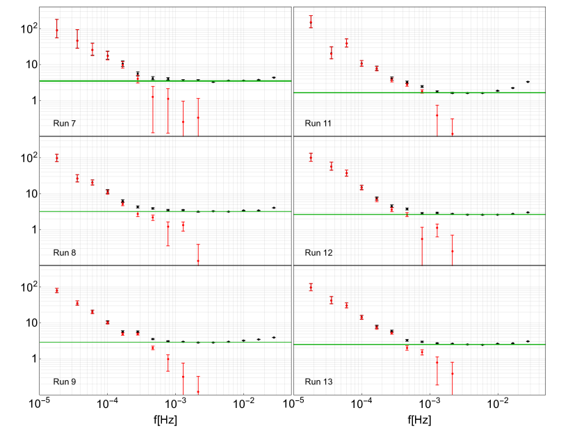
Appendix E Calculation of gravitational long-term variations

E.1 Instrument distortion

As already said in Sec. V.6, the capacitive motion sensor gives a measurement of the relative motion of the GRS relative to its own test mass, $x_{\text{GRS},i}=x_{i}-X_{i}$. Here the suffix $i$ indicates the test mass, and $X_{i}$ is the coordinate of the GRS surrounding TM$i$.

As we are only interested in time variations of differences of coordinates, here the reference frame may be taken that of the spacecraft, and each coordinate is zero at the nominal position of the body it belongs to, that is, at the position of the body in the absence of distortion.

The variation of gravitational field due to such distortion-induced motion of both GRS and the TMs can be written as:

$$\begin{split}&\Delta g_{\text{Dist},0}=\\ &-\omega_{2,2}^{2}\left(x_{2}-X_{2}\right)-\omega_{\text{SC},2}^{2}x_{2}-\omega_{2,1}^{2}\left(x_{2}-X_{1}\right)+\\ &+\omega_{1,1}^{2}\left(x_{1}-X_{1}\right)+\omega_{\text{SC},1}^{2}x_{1}+\omega_{1,2}^{2}\left(x_{1}-X_{2}\right)\end{split}$$ (31)

Here $-\omega_{i,j}^{2}$ is the force gradient (per unit mass) caused by GRS $j$ on TM $i$ and $-\omega_{\text{SC},i}^{2}$ is that caused by all the remaining parts of the spacecraft, mostly the OMS, on TM $i$. Notice that $\omega_{i}^{2}$ in Eq. (1) is given by $\omega_{i}^{2}=\left(\omega_{i,i}^{2}+\omega_{\text{SC},i}^{2}+\omega_{i,j}^{2}\right)$.

Within this model the $\Delta g$ time series is expected to be affected by a distortion-induced component:

$$\begin{split}&\Delta g_{\text{Dist}}=\Delta g_{\text{Dist},0}+\omega_{2}^{2}\left(x_{2}-x_{1}\right)+\left(\omega_{2}^{2}-\omega_{1}^{2}\right)x_{1}=\\ =&\left(\omega_{2,2}^{2}-\omega_{2,1}^{2}\right)X_{2}-\left(\omega_{1,1}^{2}-\omega_{1,2}^{2}\right)X_{1}\simeq\\ &+\simeq\left(\omega_{2,2}^{2}-\omega_{2,1}^{2}\right)\left(X_{2}-X_{1}\right)\end{split}$$ (32)

The last simplification comes from the fact that, due the symmetry of the instrument, $\left(\omega_{2,2}^{2}-\omega_{2,1}^{2}\right)\simeq\left(\omega_{1,1}^{2}-\omega_{1,2}^{2}\right)$ within the same accuracy within which $\omega_{1}^{2}\simeq\omega_{2}^{2}$, as discussed in Sec. II.2.

The relative motion of the two GRS, $\Delta x=X_{2}-X_{1}$, can be obtained as

$$\begin{split}&\Delta X=X_{2}-X_{1}=\Delta x_{\text{OMS}}-\Delta x_{\text{GRS}}=\\ &=x_{2}-x_{1}-\left(\left(x_{2}-X_{2}\right)-\left(x_{1}-X_{1}\right)\right)\end{split}$$ (33)

Thus, in conclusion,

$$\begin{split}&\Delta g_{\text{Dist}}=\\ &=\left(\omega_{2,2}^{2}-\omega_{2,1}^{2}\right)\left(\Delta x_{\text{OMS}}-\Delta x_{\text{GRS}}\right)\equiv\\ &\equiv\omega_{d}^{2}\left(\Delta x_{\text{OMS}}-\Delta x_{\text{GRS}}\right)\end{split}$$ (34)

$\omega_{2,2}^{2}$ is dominated by both gravitational and electrical effects [18], while the origin of $\omega_{2,1}^{2}$ is just gravitational. We can get an estimate of the electrical terms from [18], while the gravitational components have been estimated in [60], within the work to suppress the gravitational field at the TM location [11].

Based on these references, we calculate $\omega_{d}^{2}=(-3.32\pm 0.05)\times 10^{-7}\leavevmode\nobreak\ \text{s}^{-2}$.

E.2 Propellant tank depletion

The sign and the magnitude of $\Delta g_{\text{Tanks}}$ depends on the specific tanks from which the propellant is taken. Tank 1 and 2 of Table 2 in App. A, produce, respectively, a $\Delta g_{\text{Tanks}}$ of $\lambda_{t,1}\simeq+39\text{\,pm s}^{-2}\text{ kg}^{-1}$ and $\lambda_{t,2}\simeq+37\text{\,pm s}^{-2}\text{\,kg}^{-1}$ per unit mass of contained propellant, while for tank 3 this figure is instead $\lambda_{t,3}\simeq-43\text{\,pm\,s}^{-2}\text{\,kg}^{-1}$. These figures are the result of a numerical calculation on the geometry and location of the tanks, and are affected by a relative error of $\simeq 5\%$.

The mass loss is monitored by set of flow-meters, one for each of the thrusters, that measure the instantaneous flow of mass through that thruster. As the thrusting system contains two branches (see App. A), the measurement of the total flow of mass from the tank in use during any given run, $\dot{m}$, is the sum of the readings of the six flow-meters of the thrusters belonging to the branch in use during that specific run. We estimate an absolute accuracy on $\dot{m}$, for both branches, of the order of 10%.

From the figures above, one can estimate $\Delta g_{\text{Tank}}$, during a specific run that uses tank $i$ and branch $j$, as

$$\begin{split}&\Delta g_{\text{Tank}}(t)=\kappa_{t,i}\;\lambda_{t,i}\;\kappa_{b,j}\left(m_{j}(0)-\int_{0}^{t}\dot{m}_{j}(t)dt\right)\equiv\\ &\equiv\kappa_{t,i}\kappa_{b,j}\Delta g_{\text{Tank},0,i,j}(t)+c\end{split}$$ (35)

Here we have introduced:

• a calibration factor $\kappa_{t,i}$ for the gravitational gradient of tank $i$.

• a calibration factor $\kappa_{b,j}$ for the reading $\dot{m}_{\text{j}}(t)$ of the mass outflow from tank $j$,

• the initial propellant mass $m_{j}(0)$,

• the nominal signal $\Delta g_{\text{Tank},0,i,j}(t)=-\lambda_{t,i}\int_{0}^{t}\dot{m}_{j}(t)dt$,

• the constant $c=\lambda_{t,i}\kappa_{t,i}\kappa_{b,j}m_{j}(0)$ that has no relevance for the discussion.

In Sec. V.6 we discuss both the nominal case $\kappa_{t,i}=\kappa_{b,j}=1$ and some other options.

E.3 Drift evaluation procedure

On the long time scale of days or more we are considering here, all data series have strong auto-correlation. Thus the linear square fitting to data, that we do to estimate the residual drift, does not allow a consistent and unbiased estimate of errors. To partially circumvent this limitation we have resorted to the following procedure.

• We chose the values for $\kappa_{t,i}$, $\kappa_{b,j}$ and $\omega_{d}^{2}$. One obvious choice is $\kappa_{t,i}=\kappa_{b,j}=1$ for all values of i and j, and $\omega_{d}^{2}=-3.32\times 10^{-7}\text{\,s}^{-2}$ that we call the nominal calibration.

• For each run, we partition all relevant data series into one day-long non-overlapping stretches. Let us call $N_{k}$ the resulting number of stretches for run $k$

• For each of the stretches in one run, we form the ‘corrected’ data series $\Delta g_{c}(t)=\Delta g(t)-\kappa_{t,i}\kappa_{b,j}\Delta g_{\text{Tank},0,i,j}(t)-\omega_{d}^{2}\left(\Delta x_{\text{OMS}}-\Delta x_{\text{GRS}}\right)$, using the proper values for tank $i$ and branch $j$ used in that same run.

• Again for each of the stretches in one run, we perform a least square fitting of $\Delta g_{c}(t)$ with the model

  $$\Delta g_{c}(t)=c_{T}T+c_{t}t+\text{c}$$ (36)

• From the $N_{k}$ long sample of fitting coefficient pairs $c_{T,j},\;c_{t,j}$, with $1\leq j\leq N_{k}$, obtained by fitting the $N_{k}$ stretches of run $k$, we form the average partial derivatives $\left(\partial\Delta g/\partial T\right)_{k}\equiv(1/N)\sum_{k=1}^{N}c_{T,k}$ and $\left(\partial\Delta g/\partial t\right)_{k}\equiv(1/N)\sum_{k=1}^{N}c_{t,k}$, and the corresponding variances $\sigma_{T,k}^{2}$ and $\sigma_{t,k}^{2}$.

• As $N_{k}$ is quite small for many of the runs, to get a more solid estimate of the mean fluctuation of a single determination of coefficients, we make a weighted average over the variance on the entire set of run:

  $$\begin{split}&\sigma_{T}=\sqrt{\frac{\sum_{k=1}^{13}\left(N_{k}-1\right)\sigma_{T,k}^{2}}{\sum_{k=1}^{13}\left(N_{k}-1\right)}}\\ &\sigma_{t}=\sqrt{\frac{\sum_{k=1}^{13}\left(N_{k}-1\right)\sigma_{t,k}^{2}}{\sum_{k=1}^{13}\left(N_{k}-1\right)}}\end{split}$$

• Finally, we take $\sigma_{T}/\sqrt{N_{k}}$ and $\sigma_{t}/\sqrt{N_{k}}$ as the uncertainty on $\left(\partial\Delta g/\partial T\right)_{k}$ and $\left(\partial\Delta g/\partial t\right)_{k}$ respectively

It is worth stressing that such a procedure remains largely empirical, and that coefficients from stretches within the same run may still be correlated so that the errors may be still underestimated. However the main results of the discussion in Sec. V.6 should depend only weakly on the details of the procedure.

Appendix F In-band noise from instrument distortion and thermal effects

In Sec. VIII.2.1, we discussed the in-band contribution to $\Delta g$ of the instrument distortion and thermal effects. Here we give details and calculations.

Susceptibilities — A set of thermal experiments [61] has shown the possibility of delay effects between $T$ and the other time series, reasonably represented by a simple pole filter with a cut-off frequency in the $\mathrm{\SIUnitSymbolMicro Hz}$ range. We summarise all this information, by taking the following distributions for the susceptibilities:

• $\omega_{d}^{2}$ is frequency-independent and normally distributed with $\omega_{d}^{2}=(-0.33\pm 0.03)\times 10^{-6}\,$\mathrm{s}^{-2}$$.

• $\alpha_{T}(f)$, the susceptibility of $\Delta g$ to $T$, is given by $\alpha_{T}(f)=\alpha_{T,0}\left(1+if/f_{0}\right)^{-1}$, with $\alpha_{T,0}$ normally distributed with $\alpha_{T,0}=(0.4\pm 0.2)\,$\mathrm{p}\mathrm{m}\,\mathrm{s}^{-2}\,\mathrm{K}^{-1}$$, and $\log f_{0}$ uniformly distributed between of $\log($1\text{\,}\mathrm{\SIUnitSymbolMicro Hz}$)$ and $\log($100\text{\,}\mathrm{\SIUnitSymbolMicro Hz}$)$.

• $\gamma(f)$, the susceptibility of $\Delta X$ to $T$, is given by $\gamma(f)=\gamma_{0}\left(1+if/f_{1}\right)^{-1}$, with $\gamma_{0}$ normally distributed with $\gamma_{0}=(1.04\pm 0.07)\,$\mathrm{\SIUnitSymbolMicro}\mathrm{m}\,\mathrm{K}^{-1}$$, and $f_{1}$ with the same distribution as for $f_{0}$.

First approach — The first obvious, naive way to put an upper limit to the combined contribution of $\Delta g_{\text{Dist}}$ and $\Delta g_{T}$ to the PSD of $\Delta g$, is to: assume that these are not affected by any readout noise; take the posterior for the joint CPSD of $\Delta X$, $\Delta T$ and $\Delta g$ from the proper distribution, as explained in App. B.3.1; take the posterior for the susceptibilities as explained above. From all this, the total contribution to $S_{\Delta g}$ of $\Delta X$ and $\Delta T$ would be

$$\omega_{d}^{4}S_{\Delta X}(f)+\left(2\text{Re}\left[\omega_{d}^{2}\alpha_{T}(f)\gamma^{*}(f)\right]+\lvert\alpha_{T}(f)\rvert^{2}\right)S_{T}(f),$$ (37)

Second approach — A more informative bound can be obtained explicitly including the presence of the readout noise affecting the time series. We include the following considerations:

1. The measured $\Delta X$ and $T$ are affected by unmodeled and uncorrelated readout noises. Moreover, the noise affecting $\Delta X$ correlates to $\Delta g_{0}$ in Eq. (15).

2. $\Delta\Phi$ is also affected by readout noise, which correlates with $\Delta X$.

3. The angular distortion $\Delta\Phi$ has a negligible contribution to the linear acceleration noise $\Delta g$.

We define the matrices $\bm{\Sigma}_{\Delta X}$, $\bm{\Sigma}_{T}$, and $\bm{\Sigma}_{0}$ so that the CPSD matrix of $(\Delta g,\Delta X,T,\Delta\Phi)$ can be written as

$$\bm{\Sigma}=\bm{\Sigma}_{0}+S_{\Delta X}\bm{\Sigma}_{\Delta X}+S_{T}\bm{\Sigma}_{T}+S_{\Delta\Phi}\bm{\Sigma}_{\Delta\Phi}$$ (38)

Here, $\bm{\Sigma}_{0}$ represents the CPSD between $\Delta g_{0}$ and the readout noise part of $\Delta X$, $T$, and $\Delta\Phi$. According to the previous assumptions, the matrices read

$$\begin{split}&\bm{\Sigma}_{T}=\left(\begin{matrix}|\alpha_{T}|^{2}+2\text{Re}\left(\alpha_{T}\omega_{d}^{2}\gamma^{*}\right)&\alpha_{T}\gamma^{*}&\omega_{d}^{2}\gamma+\alpha_{T}&0\\ \alpha_{T}^{*}\gamma&0&\gamma&0\\ \omega_{d}^{2}\gamma^{*}+\alpha_{T}^{*}&\gamma^{*}&1&0\\ 0&0&0&0\end{matrix}\right)\\ &\bm{\Sigma}_{\Delta X}=\left(\begin{matrix}\omega_{d}^{4}&\omega_{d}^{2}&0&0\\ \omega_{d}^{2}&1&0&0\\ 0&0&0&0\\ 0&0&0&0\end{matrix}\right)\end{split}$$ (39)

Within this model, we estimate the contribution to $S_{\Delta g}$. First, we take a sample from the posterior of $\bm{\Sigma}$ (see App. B.3.1) and one from that of the susceptibilities, from which we build $\bm{\Sigma}_{0}$ using Eqs. (38) and (39). Then, we search the values of $S_{\Delta X}$, $S_{T}$, and $S_{\Delta\Phi}$ that give the maximum noise contribution $\left(S_{\Delta X}\bm{\Sigma}_{\Delta X}+S_{T}\bm{\Sigma}_{T}\right)_{1,1}$, subject to the condition that $\bm{\Sigma}_{0}$ is a positive definite matrix, as a CPSD should always be. We repeat the calculation over a thousand different posterior samples, deriving a posterior also for this upper limit. The result is in Fig. 16 on page 16.

Appendix G Noise from Poisson flow of glitches

A very simple model for a stochastic process that shows a $1/f$ ASD, is a flow of steps $\Delta g(t)=g_{i}\Theta(t-t_{i})$, with $\Theta(t)$ the Heaviside theta function, $g_{i}$ a random amplitude, and with the arrival times $t_{i}$ following Poisson event statistics. Such a process has indeed an ASD given by $S_{\Delta g}^{1/2}=\sqrt{2\lambda\langle g_{i}^{2}\rangle/(2\pi f)^{2}}$, with $\lambda$ the event rate.

The process can be generalized. Specifically, one can calculate the ASD of a flow of Poisson events $\Delta g(t)=g_{i}h_{i}(t-t_{i})\Theta(t-t_{i})$, with $h_{i}(t)$ the unit peak amplitude version of a randomly selected glitch among those observed during ordinary LPF noise runs [20]. As we only observed $N_{g}=98$ glitches, to generate an arbitrary long time series, in this process glitch shapes need to be repeated.

The PSD of such a process would be

$$S_{\Delta g,gl}(f)^{1/2}=\sqrt{2\lambda\langle g_{i}^{2}\rangle\frac{1}{N_{g}}\sum_{l=1}^{N_{g}}\lvert h_{l}(f)\rvert^{2}},$$ (40)

Here $h_{l}(t)$ is the shape of the $l$-th observed glitch, and $h_{l}(f)$ its Fourier transform. For the sake of the current discussion all 98 glitches had $h_{l}(t)\propto e^{-t/\tau_{2,l}}-e^{-t/\tau_{1,l}}$ with $\tau_{2,l}$ and $\tau_{1,l}$ two time constants [20].

Figure 27 compares the ASD calculated from Eq. (40) taking $2\lambda\langle g_{i}^{2}\rangle=9.8\times 10^{-5}\text{\,fm}^{2}\text{s}^{-5}$ (the dashed black line), to data from run 10 (the black dots). To ease the comparison, the figure reports $\sqrt{S_{\Delta g,gl}+S_{\text{Brown}}}$, with $S_{\text{Brown}}$ the maximum likelihood value for run 10.

FIG. 27: ASD from a Poisson flow of glitches. Dashed black line: calculated ASD of a flow of glitches taken at random from the sample of the observed ones and with $2\lambda\langle g_{i}^{2}\rangle=9.8\times 10^{-5}\text{\,fm}^{2}\text{s}^{-5}$ (see text for definition of symbols). Blue dot-dashed line: calculated ASD of a flow of glitches with time parameters taken at random from the extended distribution described in the text and with $2\lambda\langle g_{i}^{2}\rangle=8.0\times 10^{-5}\,\text{fm}^{2}\text{s}^{-5}$. Red dots: ASD of a simulated time series with the same length as that of run 10, with glitch parameters extracted from the extended simulation, $g_{i}$ extracted from a uniform distribution in the interval $\pm 0.9\,\text{fm\,s}^{-2}$, and with a rate of $\lambda=105\,\text{d}^{-1}$.

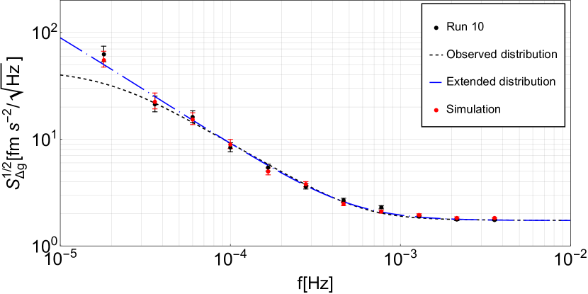
It must be said the indistinguishable results, except for the numerical value of $2\lambda\langle g_{i}^{2}\rangle$, are obtained by taking just the 54 glitches for which $\tau_{2,l},\tau_{1,l}\geq 10\,\text{s}$.

The figure shows that such a simple model may well be fit to the observed ASDs, at least for frequencies $f\gtrsim$30\text{\,}\mathrm{\SIUnitSymbolMicro Hz}$$. However below that limit the predicted ASD saturate, as none of the observed time constants ever exceeded $\simeq 8\,\text{ks}$ [20]. To achieve a better result one needs then to slightly extend the family of templates $h(t)$.

To do that, we first note that more than 90% of the glitches for which $\tau_{2,l},\tau_{1,l}\geq 10\,\text{s}$, had $\tau_{2,l}=\tau_{1,l}\equiv\tau_{l}$, a case in which $h_{l}(t)\to e(t/\tau_{l})e^{-t/\tau_{l}}$. For these glitches the distribution of $\log_{10}(\tau_{l}/1\,\text{s})$ is quantitatively compatible with a uniform one in the range 1 to 4.

The simplest model extension is then to a flow of glitches of the kind $\Delta g(t)=g_{i}e(t/\tau_{i})e^{-t/\tau_{i}}\Theta(t-t_{i})$ with the distribution of $\log_{10}(\tau_{i}/1\,\text{s})$, extended up to 5, instead of being limited to 4.

The results for such an extended model, with a fitting constant $2\lambda\langle g_{i}^{2}\rangle=8.0\times 10^{-5}\,\text{fm}^{2}\text{s}^{-5}$ are reported again in Fig. 27 (blue dot-dashed line).

We now discuss the possibility that the glitches that form this hypothetical random flow, the noise glitches, may be the same that occasionally become large enough to be detected as isolated signals in the data series, the isolated glitches. To do that let us first discuss the possible parameter distribution of the noise glitches.

The model above would reproduce our observations if the values for $2\lambda\langle g_{i}^{2}\rangle$ would only refer to glitches with amplitude $g_{i}$ small enough to be undetectable against the background noise. Indeed the data series on which we have calculated noise ASD have been purged of any detectable glitch [2], and thus of their contribution to the ASD. This puts a constraint on the distribution of $g_{i}$ for the noise glitches, that depends on our ability to detect a glitch against the background noise.

Our empirical glitch detection method has been described in [20], and its detection ability found in substantial agreement with the prediction of a search based on a matched filter. We have repeated such an analysis for the amplitude normalisation we use here, calculating the joint Fisher matrix for $g_{i}$, $\tau_{1,i}$, $\tau_{2,i}$ and the glitch arrival time, and confirmed such an agreement.

Specifically all detected glitches have signal to noise ratio $\text{SNR}\geq 3.6$, with $\text{SNR}=\lvert g_{i}\rvert/\sigma_{g}$, and $\sigma_{g}$ the uncertainty on $g_{i}$ predicted by the Fisher matrix, and all but 4 have a signal to noise ratio $\text{SNR}\geq 5$. Indeed visual inspection confirms that our empirical method would detect almost certainly any glitch with $\text{SNR}=5$, while would almost certainly not detect a glitch with $\text{SNR}\leq 3.5$.

For a given amplitude $g_{i}$, SNR depends on $S_{\text{Brown}}$, but also on both $\tau_{1,i}$ and $\tau_{2,i}$. For run 10, the run with best noise, the SNR reaches a maximum for $\tau_{1,i}=\tau_{2,i}\simeq$85\text{\,}\mathrm{s}$$.

Putting all these elements together, and reminding the stability of the observed noise in the course of the mission, the distribution of $g_{i}$ and $\tau_{i}$ for the noise glitches should fulfill the following conditions:

• $g_{i}$ and $\tau_{i}$ should be independent;

• their distributions should both be independent of the run;

• $\log_{10}(\tau_{i}/1\,\text{s})$ should be uniformly distributed between 1 and 5

• the distribution of $g_{i}$ should fulfill: $2\lambda\langle g_{i}^{2}\rangle\simeq 8.0\times 10^{-5}\text{\,fm}^{2}\text{s}^{-5}$

• the distribution of $g_{i}$ should assign a probability $p_{t}$ to $g_{i}+s_{i}\geq 5\sigma_{g}$, with $s_{i}$ the random amplitude measurement error, such that $\lambda p_{t}$ is much less than the observed rate, of $\simeq 1\text{\,d}^{-1}$ of the isolated glitches. Here all quantities refer to run 10 and to $\tau_{1,i}=\tau_{2,i}\simeq 85\text{s}$ which is the most favorable case for glitch detection.

Thus the question if the isolated glitches are just a sample of large amplitude tail of an overall distribution of glitch parameters, translates in that if the amplitude distribution of the noise glitches, fulfilling the constraints above, merges at high amplitude into that of the isolated glitches, without the need of too many pathological assumptions to fill up the gaps among the two.

In order to start with the minimum such gap, in the condition for $2\lambda\langle g_{i}^{2}\rangle$ one should pick the lowest possible value for $\lambda$ corresponding to the largest for $\langle g_{i}^{2}\rangle$. Barring the non-physical assumption of all equal $g_{i}$’s, the simple distribution that maximizes $\langle g_{i}^{2}\rangle$ for a given upper bound $g_{\text{max}}$, is a uniform distribution $-g_{\text{max}}\leq g_{i}\leq g_{\text{max}}$ for which $\langle g_{i}^{2}\rangle=(1/3)g_{\text{max}}^{2}$.

To decide the value of $g_{\text{max}}$ we take the conditions of run 10, with $\tau_{1,i}=\tau_{2,i}\simeq$85\text{\,}\mathrm{s}$$, recast $g_{\text{max}}=n_{\text{max}}\sigma_{g}$, and calculate the probability that a sample from a uniform distribution $-n_{\text{max}}\sigma_{g}\leq g_{i}\leq n_{\text{max}}\sigma_{g}$, plus an independent sample from a zero-mean normal distribution with variance $s_{g}^{2}$, representing the measurement error, exceeds in absolute value, the threshold $5\sigma_{g}$. We pick $n_{\text{max}}$ when this probability is low enough to detect at most one detectable glitch in a run with the same duration of run 10. The procedure requires a few trial and error loops involving adjusting the value of $\lambda$ that try to minimize.

Figure 27 shows the ASD (red dots) of simulated data assuming $\lambda=102\text{\,d}^{-1}$, $n_{\text{max}}=3$, $\sigma_{g}=0.1\text{\,fm\,s}^{-2}$, and the Brownian noise level and the time duration of run 10. Inspection of the data shows no glitch we would have detected with our empirical method.

We have simulated noise glitches to reproduce the noise for all runs in which we have observed the glitches [20], by generating amplitudes and time constants from the same distributions, independently of the run. For each of the simulated glitches, we have also generated the amplitude that would have been measured by the matched filter, by adding a simulated measurement error, and tested if the glitch would have been detected within the specific run to which it belonged. The results of such collective simulation are shown in Fig. 28.

FIG. 28: Measured amplitude $g_{i,m}$ versus time constant $\tau_{i}$ for both simulated noise glitches and observed isolated ones. Black dots: all observed isolated glitches with $\tau_{2,i}=\tau_{1,i}\equiv\tau_{i}$ and $\tau_{i}>10\text{\,s}$. The remaining dots refer to all noise glitches from a simulation aimed at reproducing the noise ASD of all runs in which isolated glitches have been observed [20]. Red dots refer to glitches with $\text{SNR}<5$, while blue dots refer to those with $\text{SNR}\geq 5$ that would have almost certainly been detected in real data.

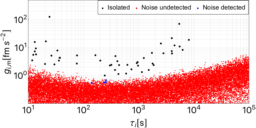
The parameter space for these simulations is rather vast, and the criterion for detectability is not free of ambiguity. Nevertheless, the picture strongly suggests that:

1. there is an abrupt, order of magnitude large jump in the probability density between the upper edge of the noise glitches distribution and that of the isolated ones;

2. there is a large void in the population of isolated glitches for $\tau_{i}\gtrsim$200\text{\,}\mathrm{s}$$, between the amplitude of the observed glitches and that of noise one. This void is real, glitches with amplitude in the void would be observable with high SNR.

3. As already noted, glitches with $\tau_{i}\geq 10^{4}\text{\,s}$, necessary to reproduce the noise, are missing in the observed sample.

These features are unlikely to disappear as a result of the tuning of any of the model details.

Thus it may be that the noise is due to a flow of undetectable glitches, but these appear to belong to a distribution so significantly separated from that of the observed ones, to make the conclusion that we may be witnessing two aspects of the same physical phenomenon, highly speculative.

It is also worth noting that, already at the minimal rate of $\lambda\simeq 100-200\text{\,d}^{-1}$, the simulated time series appear Gaussian and stationary within the statistical uncertainty, making their Poisson nature undetectable from the data. Thus again the hypothesis that $\Delta g_{e}(t)$ is Poisson in origin, remains a speculation.

References

- [1] M. Armano et al. Beyond the Required LISA Free-Fall Performance: New LISA Pathfinder Results down to . Phys. Rev. Lett., 120:061101, Feb 2018. DOI: 10.1103/PhysRevLett.120.061101.
- [2] M. Armano et al. Sub-Femto- Free Fall for Space-Based Gravitational Wave Observatories: LISA Pathfinder Results. Phys. Rev. Lett., 116:231101, 2016. DOI: 10.1103/PhysRevLett.116.231101.
- [3] Amaro-Seoane et al. Laser Interferometer Space Antenna, 2017. DOI: 10.48550/arXiv.1702.00786.
- [4] P. McNamara, S. Vitale, K. Danzmann and LISA Pathfinder Sci Working Team. LISA Pathfinder. Classical and Quantum Gravity, 25(11), 2008. DOI: 10.1088/0264-9381/25/11/114034.
- [5] M. Armano et al. Sensor Noise in LISA Pathfinder: In-Flight Performance of the Optical Test Mass Readout. Phys. Rev. Lett., 126:131103, Apr 2021. DOI: 10.1103/PhysRevLett.126.131103.
- [6] LISA Pathfinder Collaboration et al. Capacitive sensing of test mass motion with nanometer precision over millimeter-wide sensing gaps for space-borne gravitational reference sensors. Physical Review D, 96(6):062004, September 2017. DOI: 10.1103/PhysRevD.96.062004.
- [7] M. Armano et al. Spacecraft and interplanetary contributions to the magnetic environment on-board LISA Pathfinder. Monthly Notices of the Royal Astronomical Society, 494(2):3014–3027, 04 2020. DOI: 10.1093/mnras/staa830.
- [8] M. Armano et al. Temperature stability in the sub-milliHertz band with LISA Pathfinder. Monthly Notices of the Royal Astronomical Society, 486(3):3368–3379, 04 2019. DOI: 10.1093/mnras/stz1017.
- [9] P. Canizares et al. The LISA Pathfinder DMU and Radiation Monitor. Classical and Quantum Gravity, 28(9):094004, 05 2011. DOI: 10.1088/0264-9381/28/9/094004.
- [10] M. Armano et al. Characteristics and Energy Dependence of Recurrent Galactic Cosmic-Ray Flux Depressions and of a Forbush Decrease with LISA Pathfinder. The Astrophysical Journal, 854(2):113, February 2018. DOI: 10.3847/1538-4357/aaa774.
- [11] M. Armano et al. Constraints on LISA Pathfinder’s self-gravity: design requirements, estimates and testing procedures. Classical and Quantum Gravity, 33(23):235015, 2016. DOI: 10.1088/0264-9381/33/23/235015.
- [12] S. Tibbitts. High-output paraffin linear motors: utilization in adaptive systems. page 388, San Diego, CA, 01 1992. DOI: 10.1117/12.51194.
- [13] M. Armano et al. LISA Pathfinder micronewton cold gas thrusters: In-flight characterization. Phys. Rev. D, 99:122003, Jun 2019. DOI: 10.1103/PhysRevD.99.122003.
- [14] L. Ferraioli, M. Hueller and S. Vitale. Discrete derivative estimation in LISA Pathfinder data reduction. Classical and Quantum Gravity, 26(9), 2009. DOI: 10.1088/0264-9381/26/9/094013.
- [15] LISA Instrument Group. LISA Performance Model and Error Budget. Technical note. LISA-LCST-INST-TN-003, 2020.
- [16] M. Armano et al. Tilt-to-length coupling in LISA Pathfinder: A data analysis. Phys. Rev. D, 108:102003, Nov 2023. DOI: 10.1103/PhysRevD.108.102003.
- [17] M.S. Hartig and G. Wanner. Tilt-to-length coupling in LISA Pathfinder: Analytical modeling. Phys. Rev. D, 108:022008, Jul 2023. DOI: 10.1103/PhysRevD.108.022008.
- [18] M. Armano et al. Calibrating the system dynamics of LISA Pathfinder. Phys. Rev. D, 97:122002, Jun 2018. DOI: 10.1103/PhysRevD.97.122002.
- [19] M. Armano et al. Analysis of the accuracy of actuation electronics in the laser interferometer space antenna pathfinder. Review of Scientific Instruments, 91(4):045003, 2020. DOI: 10.1063/1.5140406.
- [20] M. Armano et al. Transient acceleration events in LISA Pathfinder data: Properties and possible physical origin. Phys. Rev. D, 106:062001, Sep 2022. DOI: 10.1103/PhysRevD.106.062001.
- [21] M. Armano et al. Charging of free-falling test masses in orbit due to cosmic rays: Results from LISA Pathfinder. Phys. Rev. D, 107:062007, Mar 2023. DOI: 10.1103/PhysRevD.107.062007.
- [22] M. Armano et al. Charge-Induced Force Noise on Free-Falling Test Masses: Results from LISA Pathfinder. Phys. Rev. Lett., 118:171101, Apr 2017. DOI: 10.1103/PhysRevLett.118.171101.
- [23] M. Armano et al. Measuring the Galactic Cosmic Ray flux with the LISA Pathfinder radiation monitor. Astroparticle Physics, 98:28–37, 2018. DOI: 10.1016/j.astropartphys.2018.01.006.
- [24] M. Armano et al. Precision charge control for isolated free-falling test masses: LISA pathfinder results. Phys. Rev. D, 98:062001, Sep 2018. DOI: 10.1103/PhysRevD.98.062001.
- [25] A. Cavalleri et al. Increased Brownian Force Noise from Molecular Impacts in a Constrained Volume. Phys. Rev. Lett., 103:140601, Sep 2009. DOI: 10.1103/PhysRevLett.103.140601.
- [26] H. Jeffreys. An invariant form for the prior probability in estimation problems. Proceedings of the Royal Society of London. Series A. Mathematical and Physical Sciences, 186(1007):453–461, 1946. DOI: 10.1098/rspa.1946.0056.
- [27] K. Jousten, editor. Handbook of vacuum technology. Wiley-VCH Verlag GmbH & Co. KGaA, Weinheim, second, completely revised and updated edition edition, 2016. DOI: 10.1002/9783527688265.
- [28] P. Chiggiato. Outgassing properties of vacuum materials for particle accelerators, 2020. DOI: 10.48550/arXiv.2006.07124.
- [29] LISA Science Study Team. LISA Science Requirements Document. ESA-L3-EST-SCI-RS-001 1.0, May 2018.
- [30] H. Akaike. A new look at the statistical model identification. IEEE Transactions on Automatic Control, 19(6):716–723, 1974. DOI: 10.1109/TAC.1974.1100705.
- [31] A. Gelman et al. Bayesian Workflow, 2020. DOI: 10.48550/arXiv.2011.01808.
- [32] M. Armano et al. NanoNewton electrostatic force actuators for femtoNewton-sensitive measurements: system performance test in the LISA Pathfinder mission. 2024. In print, Phys. Rev. D, DOI: 10.48550/arXiv.2401.00884.
- [33] P.A. Redhead. Modeling the pumpdown of a reversibly adsorbed phase. I. Monolayer and submonolayer initial coverage. Journal of Vacuum Science & Technology A, 13(2):467–475, 1995. DOI: 10.1116/1.579381.
- [34] R. Kersevan and M. Ady. Recent Developments of Monte-Carlo Codes Molflow+ and Synrad+. In Proc. 10th International Particle Accelerator Conference (IPAC’19), Melbourne, Australia, 19-24 May 2019, number 10 in International Particle Accelerator Conference, pages 1327–1330, Geneva, Switzerland, Jun. 2019. JACoW Publishing. DOI: doi:10.18429/JACoW-IPAC2019-TUPMP037.
- [35] M. Armano et al. Sensor noise in LISA Pathfinder: An extensive in-flight review of the angular and longitudinal interferometric measurement system. Phys. Rev. D, 106:082001, Oct 2022. DOI: 10.1103/PhysRevD.106.082001.
- [36] S. Vitale. Possible excess GRS sensing noise with TM in science mode. S2-UTN-TN-3151 1.0, 2018.
- [37] Y. Levin. Creep events and creep noise in gravitational-wave interferometers: Basic formalism and stationary limit. Phys. Rev. D, 86:122004, Dec 2012. DOI: 10.1103/PhysRevD.86.122004.
- [38] F. Antonucci et al. Interaction between Stray Electrostatic Fields and a Charged Free-Falling Test Mass. Physical Review Letters, 108(18):5, 2012. DOI: 10.1103/PhysRevLett.108.181101.
- [39] LISA Pathfinder collaboration. Magnetic-induced force noise in LISA Pathfinder free-falling test masses. In preparation, 2024.
- [40] LISA Pathfinder collaboration. Precision measurements of the magnetic parameters of LISA Pathfinder test masses. In preparation, 2024.
- [41] L. Carbone et al. Thermal gradient-induced forces on geodesic reference masses for LISA. Phys. Rev. D, 76:102003, Nov 2007. DOI: 10.1103/PhysRevD.76.102003.
- [42] B. Kaune. In-orbit stability analysis of the LISA pathfinder optical metrology: photoreceivers and polarisation. PhD thesis, Hannover: Gottfried Wilhelm Leibniz Universität, 2021. DOI: 10.15488/10887.
- [43] T.W. Darling, F. Rossi, G.I. Opat and G.F. Moorhead. The fall of charged particles under gravity: A study of experimental problems. Rev. Mod. Phys., 64:237–257, Jan 1992. DOI: 10.1103/RevModPhys.64.237.
- [44] S. Vitale, L. Sala, V. Ferroni and W.J. Weber. Estimate of force noise from electrostatic patch potentials in lisa pathfinder, 2024. DOI: https://doi.org/10.48550/arXiv.2404.08340.
- [45] M. Brownnutt, M. Kumph, P. Rabl and R. Blatt. Ion-trap measurements of electric-field noise near surfaces. Rev. Mod. Phys., 87:1419–1482, Dec 2015. DOI: 10.1103/RevModPhys.87.1419.
- [46] G. Russano et al. Measuring fN force variations in the presence of constant nN forces: a torsion pendulum ground test of the LISA Pathfinder free-fall mode. Classical and Quantum Gravity, 35(3):035017, 02 2018. DOI: 10.1088/1361-6382/aaa00f.
- [47] H.D. Wealthy and W. C. Spacecraft-Level Gravity Model Results. S2.ASU.TN.2270.ISS02, 2008.
- [48] B. Schläppi et al. Influence of spacecraft outgassing on the exploration of tenuous atmospheres with in situ mass spectrometry. Journal of Geophysical Research: Space Physics, 115(A12), 2010. DOI: 10.1029/2010JA015734.
- [49] F. Antonucci et al. From laboratory experiments to LISA Pathfinder: achieving LISA geodesic motion. Classical and Quantum Gravity, 28(9):094002, 2011. DOI: 10.1088/0264-9381/28/9/094002.
- [50] C. Zanoni and V. Ferroni. Electromagnetic shielding effect of the Electrode Housing. LISA-UTN-INST-TN-022 Iss. 1.1, 2024.
- [51] H.D. Wealthy and T. C. Prediction of spacecraft magnetic field based on recent testing. S2.ASU.TN.2523.ISS03, 2011.
- [52] G. Anderson et al. Experimental results from the ST7 mission on LISA Pathfinder. Phys. Rev. D, 98:102005, Nov 2018. DOI: 10.1103/PhysRevD.98.102005.
- [53] S. Vitale et al. Data series subtraction with unknown and unmodeled background noise. Phys. Rev. D, 90:042003, 2014. DOI: 10.1103/PhysRevD.90.042003.
- [54] P.D. Welch. The use of fast Fourier transform for the estimation of power spectra: a method based on time averaging over short, modified periodograms. IEEE Trans. Audio and Electroacoustics, 15(2):70–73, 1967. DOI: 10.1109/TAU.1967.1161901.
- [55] N.R. Goodman. Statistical Analysis Based on a Certain Multivariate Complex Gaussian Distribution (An Introduction). The Annals of Mathematical Statistics, 34(1):152–177, March 1963. DOI: 10.1214/aoms/1177704250.
- [56] P. Shaman. The inverted complex Wishart distribution and its application to spectral estimation. J. Multivar. Anal., 10(1):51–59, March 1980. DOI: 10.1016/0047-259X(80)90081-0.
- [57] L. Svensson and M. Lundberg. On posterior distributions for signals in Gaussian noise with unknown covariance matrix. IEEE Transactions on Signal Processing, 53(9):3554–3571, 2005. DOI: 10.1109/TSP.2005.853102.
- [58] C. Villegas. On the A Priori Distribution of the Covariance Matrix. The Annals of Mathematical Statistics, 40(3):1098 – 1099, 1969. DOI: 10.1214/aoms/1177697617.
- [59] J. Ellis and R. van Haasteren. jellis18/PTMCMCSampler: Official Release, October 2017. DOI: 10.5281/zenodo.1037579.
- [60] P. Sarra. LISA Technology Package Core Assembly Gravitational Analysis Report. S2-CGS-RP-3001. Iss10, 2015.
- [61] M. Armano et al. Temperature-induced forces on geodesic reference masses for LISA: results from LISA Pathfinder. In preparation, 2024.