MIDGARD: Self-Consistency Using Minimum Description Length
for Structured Commonsense Reasoning

Abstract

We study the task of conducting structured reasoning as generating a reasoning graph from natural language input using large language models (LLMs). Previous approaches have explored various prompting schemes, yet they suffer from error propagation due to the autoregressive nature and single-pass-based decoding, which lack error correction capability. Additionally, relying solely on a single sample may result in the omission of true nodes and edges. To counter this, we draw inspiration from self-consistency (SC), which involves sampling a diverse set of reasoning chains and taking the majority vote as the final answer. To tackle the substantial challenge of applying SC on generated graphs, we propose MIDGARD (MInimum Description length Guided Aggregation of Reasoning in Directed acyclic graph) that leverages Minimum Description Length (MDL)-based formulation to identify consistent properties among the different graph samples generated by an LLM. This formulation helps reject properties that appear in only a few samples, which are likely to be erroneous, while enabling the inclusion of missing elements without compromising precision. Our method demonstrates superior performance than comparisons across various structured reasoning tasks, including argument structure extraction, explanation graph generation, inferring dependency relations among actions for everyday tasks, and semantic graph generation from natural texts.

MIDGARD: Self-Consistency Using Minimum Description Length
for Structured Commonsense Reasoning

Inderjeet Nair  and Lu Wang University of Michigan, Ann Arbor, MI {inair, wangluxy}@umich.edu

Figure 1: Comparison of MIDGARD with CoCoGen. In this example, our objective is to infer dependency relations among items in the "Action List" to achieve the specified "Objective". CoCoGen uses greedy decoding and exhibits errors in the output, e.g., "decided to run errands during a break in the rain" is not connected with "Drive to errand location and complete". In contrast, our approach MIDGARD (within the orange rectangle) aggregates relevant information across different samples, resulting in more accurate inference. For this example, our algorithm improved the performance of greedy decoding from $\mathbf{66.7}$ to $\mathbf{85.7}$ in edge $F_{1}$-score.

1 Introduction

While large language models (LLMs) have showcased impressive performance in few-shot/zero-shot scenarios across diverse reasoning tasks Brown et al. (2020); Chen et al. (2021); Rae et al. (2022); Hoffmann et al. (2022); Chowdhery et al. (2022), it is still challenging to apply these models for structured commonsense reasoning which involves generating task-specific reasoning as a graph, such as extracting argument structures from argumentative text Stab and Gurevych (2017); Hua et al. (2019); Mayer et al. (2020); Hua and Wang (2022); Qiao et al. (2022), generating structured explanations that lay out commonsense knowledge to connect an argument to a belief Saha et al. (2021), and inferring dependencies among events for everyday activities Sakaguchi et al. (2021).

There are two main challenges for structured reasoning tasks. (1) Style discrepancy: Conventional approaches for structured response generation represent the graphs as flattened strings Madaan and Yang (2021); Madaan et al. (2021); Sakaguchi et al. (2021); Saha et al. (2021), leading to subpar performance due to output style mismatch Madaan et al. (2022). (2) Error propagation: Any incorrect decisions made earlier in the autoregressive decoding process can influence later generation steps Yao et al. (2023). Recently, Madaan et al. (2022) propose CoCoGen to address the issue of style mismatch in structured reasoning tasks, by using programming scripts as prompts for LLMs. It still suffers from error propagation, since it generates variable declarations and function calls in order to describe the nodes and edges within the graph. Any error in these declarations/calls can affect the subsequent generations.

To address these issues, we take inspiration from the self-consistency (SC) Wang et al. (2023b) strategy that samples diverse reasoning paths and then takes a majority vote as the final answer. The intuition behind SC is that sampling distinct reasoning chains leads to higher confidence in the correctness of a consistent answer. Therefore, we hypothesize that sampling diverse graphs from an LLM can construct a more accurate aggregate graph and alleviate error propagation for structured reasoning tasks as any errors made in one sample are less likely to persist across all the generated graphs.

A crucial distinction between SC and our desideratum is that SC focuses exclusively on commonsense reasoning tasks Ling et al. (2017); Clark et al. (2018); Cobbe et al. (2021); Patel et al. (2021); Geva et al. (2021) with scalar answer spaces. In contrast, we aim to merge multiple graphs, each representing a collection of unordered sets (nodes and edges). It is unclear how to apply majority vote to aggregate distinct sets of nodes and edges. In particular, it would be critical to filter out inaccurate nodes and edges in our setup.

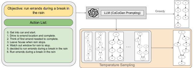
To achieve this, we propose MIDGARD, based on MInimum Description length Guided Aggregation of Reasoning in Directed acyclic graph. We employ the principle of minimum description length (MDL) Rissanen (1978) which seeks to find the hypothesis with shortest description length of the observations. While MDL has been implemented for model selection Grünwald (2005), causal structure learning Lam and Bacchus (1993, 1994), data clustering Rissanen (2000), and dimensionality reduction Bruni et al. (2022), to the best of our knowledge, its use in automatically merging graph samples has never been explored before. Assuming that graph properties consistent across multiple generated samples are more likely to be accurate, we define the description length of a graph sample as the weighted sum of the transformations required to convert a hypothesis into the given sample. By constructing a hypothesis that minimizes the description length across all the generated samples, our solution encourages the inclusion of graph properties that were present in many samples, while rejecting properties that were only present in a few samples which are likely to be erroneous. Figure 1 shows an example of how our approach reduces errors compared to relying solely on a single greedy generation. Empirical results on four different structured reasoning tasks, including argument structure extraction, structured explanation construction, and goal-oriented script generation and semantic graph generation, on eight benchmarks show that MIDGARD can outperform competitive baseline and model variants, demonstrating its strong generalizability.

2 Background and Notations

In structured reasoning, a labeled data point is denoted as $(\mathcal{T},\mathcal{G})$, where $\mathcal{T}$ represents the input and $\mathcal{G}$ is the task-specific graph output that captures the necessary reasoning knowledge. For example, in the task of argumentative structure extraction Stab and Gurevych (2017), $\mathcal{T}$ can be an essay, and $\mathcal{G}$ represents the associated argumentative structure.

To solve this task, we employ LLM in the few-shot prompting mode where $N$ labelled data-points $\{\mathcal{T}_{i},\mathcal{G}_{i}\}_{i=1}^{N}$ are fed as in-context prompt to the model to infer the output for a test input $\mathcal{T}$. In accordance with the CoCoGen approach, we construct the in-context prompt as follows: $p=\mathcal{T}_{1}\,\oplus\,\mathcal{G}_{1}^{c}\,\cdot\,\mathcal{T}_{2}\,\oplus\,\mathcal{G}_{2}^{c}\,\cdot\,\dots\,\cdot\,\mathcal{T}_{N}\,\oplus\,\mathcal{G}_{N}^{c}$ where $\mathcal{G}_{i}^{c}$ is a semantically equivalent representation of $\mathcal{G}_{i}$ written in a generally purpose programming language like Python and $\cdot$ ($\oplus$) represents inter (intra)-instance separator. $\mathbb{P}_{c}\left(\cdot,\mathcal{T}\right)$ represents the generative distribution of the LLM for the prompt $p$ and $\mathcal{T}$. While CoCoGen relies on a single generation obtained from $\mathbb{P}_{c}\left(\cdot,\mathcal{T}\right)$, our approach utilizes this to generate multiple graph samples $\{\mathcal{G^{\prime}}_{i}\}_{i=1}^{T}\sim\mathbb{P}_{c}\left(\cdot,\mathcal{T}\right)$ and then aggregates them into a single output $\mathcal{G}$. Our novelty lies in the development of a novel and generic aggregation algorithm for the task of reasoning graph generation. This algorithm leads to significantly improved performance across multiple tasks.

3 The MIDGARD Method

MIDGARD is based on the principle of minimum description length (MDL), which succinctly captures the regularities in the given data by finding the hypothesis with the shortest description length. In graph aggregation, MDL can be used as a self-consistency strategy to merge multiple reasoning graph samples into a single aggregate graph. The core idea is to define a description length for each graph sample, which is proportional to the number of transformations required to convert a hypothesis into the given sample. By minimizing the description length for samples $\{\mathcal{G}^{\prime}_{i}\}_{i=1}^{T}$, MDL encourages the inclusion of graph properties that are common across different samples. This means that properties that appear frequently in the generated samples are more likely to be accurate and reflect the underlying structure. Conversely, properties that are only present in a few samples tend to be wrong.

In many structured reasoning tasks, the graphs typically do not have singleton nodes. For example, in argumentative structures of essays Stab and Gurevych (2017), nodes are either supported or attacked by other nodes, or they themselves support or attack other nodes. We begin by defining the description length of a graph $\mathcal{G}^{\prime}$ based on the hypothesis $\mathcal{G}$ when the graphs do not contain singleton nodes in §3.1. Next, we derive the expression for the expected description length in §3.2 assuming that $\mathcal{G}^{\prime}$ is sampled from an LLM. Based on this, we formulate an objective that aims to minimize the expected description length of the sampled graphs $\{\mathcal{G^{\prime}}_{i}\}_{i=1}^{T}\sim\mathbb{P}_{c}\left(\cdot,\mathcal{T}\right)$ in §3.3. We conclude this section by proposing modifications to the objective to address the scenario where the graph can have singleton nodes in §3.4.

3.1 Defining Description Length

We define description length of $\mathcal{G}^{\prime}$ w.r.t. hypothesis graph $\mathcal{G}$ as follows:

$$\Delta_{\mathbf{E}}(\mathcal{G}^{\prime},\mathcal{G},\lambda)=\lambda\cdot a+(1-\lambda)\cdot d$$ (1)

where $a$ represents the number of new edges to be added to $\mathcal{G}$, and $d$ is the number of edges to be deleted from $\mathcal{G}$ to convert it to $\mathcal{G}$’. We introduce the hyperparameter $\lambda$, which can be interpreted as the number of bits needed to describe a single addition, when $(1-\lambda)$ bits are needed to describe a single deletion. The subscript $\mathbf{E}$ in Eq. 1 indicates that only edge transformations are considered when calculating the description length. Since these graphs do not have isolated nodes and each node is associated with at least one edge, the description length of $\mathcal{G}^{\prime}$ can be precisely captured using edge transformations alone.

The definition in Eq. 1 is inspired by the formulation proposed by Lam and Bacchus (1994) , who applied it for refining causal graphs based on new data but not for the task of graph aggregation. While Lam and Bacchus (1994) assigned equal bit requirements for describing a single addition and deletion, our empirical results demonstrate the significance of assuming different bit requirements to achieve enhanced performance.

3.2 Expected Description Length

We denote the set of nodes and edges associated with $\mathcal{G}$ as $N(\mathcal{G})$ and $E(\mathcal{G})$ respectively. Similarly, we define $\mathbf{N}$ and $\mathbf{E}$ as the sets of all possible nodes and edges, such that each edge (node) in $\mathcal{G}^{\prime}$ and $\mathcal{G}$ belongs to $\mathbf{E}$ ($\mathbf{N}$). Taking the expectation of Eq. 1 w.r.t. $\mathcal{G}^{\prime}\sim\mathbb{P}_{c}(\dot{,}\mathcal{T})$

$$\mathbb{E}_{\mathcal{G}^{\prime}}\left[\Delta_{\mathbf{E}}(\mathcal{G}^{\prime},\mathcal{G},\lambda)\right]=\lambda\mathbb{E}_{\mathcal{G}^{\prime}}[a]+(1-\lambda)\mathbb{E}_{\mathcal{G}^{\prime}}[d]$$ (2)

$$\mathbb{E}_{\mathcal{G}^{\prime}}[a]=\mathbb{E}_{\mathcal{G}^{\prime}}\left[\sum_{e\in\mathbf{E}}\mathbbm{1}_{\{e\in E(\mathcal{G^{\prime}})\}}\cdot(1-\mathbbm{1}_{\{e\in E(\mathcal{G})\}})\right]$$ (3)

$$\mathbb{E}_{\mathcal{G}^{\prime}}[d]=\mathbb{E}_{\mathcal{G}^{\prime}}\left[\sum_{e\in\mathbf{E}}\mathbbm{1}_{\{e\notin E(\mathcal{G^{\prime}})\}}\cdot\mathbbm{1}_{\{e\in E(\mathcal{G})\}}\right]$$ (4)

After simplifying the above set of equations and representing $\mathbbm{1}_{\{e\in E(\mathcal{G})\}}$ by the binary variable $x_{e}$, we arrive at:

$$\mathbb{E}_{\mathcal{G}^{\prime}}\left[\Delta_{\mathbf{E}}(\mathcal{G}^{\prime},\mathcal{G},\lambda)\right]=\sum_{e\in\mathbf{E}}\left((1-\lambda)-\mathbb{P}_{\mathcal{G^{\prime}}}(e)\right)\cdot x_{e}+\beta$$ (6)

where $\mathbb{P}_{\mathcal{G^{\prime}}}(e)$ represents the probability of observing $e\in E(\mathcal{G^{\prime}})$ when $G^{\prime}\sim\mathbb{P}_{c}\left(\cdot,\mathcal{T}\right)$ and $\beta$ is a constant that is independent from the hypothesis $\mathcal{G}$. For each edge $e\in\mathbf{E}$, the desirability of adding $e$ to the hypothesis $\mathcal{G}$ is proportional to the difference between $\mathbb{P}_{\mathcal{G}^{\prime}}(e)$ and $(1-\lambda)$. As the probability of $e$ exceeds $(1-\lambda)$ by a larger extent, its desirability to be included in the hypothesis increases as higher probability suggests that the edge $e$ would be present in a significant number of samples, suggesting it is a consistent property. Conversely, the presence of $(1-\lambda)$ in each coefficient prevents the inclusion of edges with probabilities lower than $(1-\lambda)$ in the aggregated graph.

3.3 Hypothesis Selection

We seek to find $\mathcal{G}$ that minimizes the expected description length in Eq. 6. To estimate $\mathbb{P}_{\mathcal{G^{\prime}}}(e)$, we compute the fraction of graph samples from $\mathbb{P}_{c}(\cdot,\mathcal{T})$ that contains $e$ as one of its edges. Formally, we wish to find the following:

$$\arg\min_{\mathcal{G}}\sum_{e\in\mathbf{E}}\left((1-\lambda)-\frac{\sum_{i=1}^{T}\mathbbm{1}_{e\in E(\mathcal{G}^{\prime}_{i})}}{T}\right)\cdot x_{e}$$ (7)

In the absence of any additional constraints, identifying the structure becomes trivial—one can simply set $x_{e}$ to $1$ if its coefficient is negative, and $0$ otherwise. However, in various tasks Stab and Gurevych (2017); Saha et al. (2021); Sakaguchi et al. (2021), the graphs need to be directed acyclic graphs (DAG). Appendix B explains how to restrict the search space to DAGs when optimizing Eq. 7.

3.4 Objective for Generic Graphs

Next, we propose suitable modifications to the objective to accommodate generic graphs that may contain singleton nodes. While Eq. 1 defines the description only in terms of edge transformations, we define the description length for generic graphs as follows:

$$\Delta(\mathcal{G}^{\prime},\mathcal{G},\{\lambda_{1},\lambda_{2}\})=\Delta_{\mathbf{E}}(\mathcal{G}^{\prime},\mathcal{G},\lambda_{1})+\Delta_{\mathbf{N}}(\mathcal{G}^{\prime},\mathcal{G},\lambda_{2})$$ (8)

where $\Delta_{\mathbf{N}}$ uses the same form as Eq. 1 but calculates the description length associated with the addition and removal of nodes in order to transform $N(\mathcal{G})$ into $N(\mathcal{G^{\prime}})$. Redoing the steps described in §3.2 and §3.3 yields the following objective:

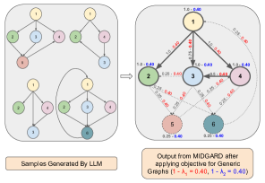
$$\arg\min_{\mathcal{G}} \sum_{e\in\mathbf{E}}\left((1-\lambda_{1})-\frac{\sum_{i=1}^{T}\mathbbm{1}_{e\in E(\mathcal{G}^{\prime}_{i})}}{T}\right)\cdot x_{e}$$ (9)

$$+ \sum_{n\in\mathbf{N}}\left((1-\lambda_{2})-\frac{\sum_{i=1}^{T}\mathbbm{1}_{n\in N(\mathcal{G}^{\prime}_{i})}}{T}\right)\cdot y_{n}$$

where $y_{n}$ is a binary variable denoting the presence of $n$ in $N(\mathcal{G})$. Note that, an edge $(n_{1},n_{2})$ can only exist if both $n_{1}$ and $n_{2}$ are present in the graph. To enforce this, we have the constraint: $\forall n_{1},n_{2}\in\mathbf{N}:y_{n_{1}}+y_{n_{2}}-2x_{(n_{1},n_{2})}\geq 0$.

Refer Figure 2 for pictorial representation of aggregation using the objective in Eq. 9.

Figure 2: Pictorial representation of Graph Aggregation. In the figure above, the probabilities of node/edge existence in a randomly generated sample from an LLM are estimated by the normalized frequency of their occurrence in the samples. The weight of an edge or node on the right-hand side is determined by subtracting $(1-\lambda_{1})$ or $(1-\lambda_{2})$ from this probability, respectively. The optimization in Eq. 9 is equivalent to the selection of the properties in the aggregated graph such that the sum of weights is maximized. The bolded elements are selected according to this maximization.

4 Experiments and Analysis

We evaluate on three major tasks for reasoning graph generation: Task 1-argument structure extraction on Essays Stab and Gurevych (2017), AbstRCT Mayer et al. (2020), and CDCP Park and Cardie (2018); Task 2-generating structured explanations on Explagraphs Saha et al. (2021); Task 3-script planning on Proscript Sakaguchi et al. (2021); and Task 4-semantic graph generation on Kelm Agarwal et al. (2021), WebNLG Gardent et al. (2017), and GenWiki Jin et al. (2020). Thereafter, we evaluate how the performance of our approach changes when using different numbers of samples generated from the LLM. Additionally, we examine the capability of our approach in handling graphs with varied complexities. Finally, we assess the influence of varying the number of few-shot examples and examine how close our automatically chosen hyperparameters are in comparison with the best possible ones. We also analyze the influence of varying the number of few-shot examples. Unless stated otherwise, we generate $T=10$ samples for approaches utilizing multiple samples.

Base LLMs. We evaluate our approach with (a) gpt-3.5-turbo, a general purpose instruction-tuned LLM and (b) Code-Llama Roziere et al. (2023), a code-LLM pretrained over general purpose programming languages. The $16$K context length associated with these LLMs allows us to employ few-shot prompting for long sequence input-output tasks such as argument structure extraction.

Comparisons. We first consider a Greedy baseline that represents each graph as a semantically equivalent programming script and samples only one generation from the LLM, which is decoded greedily as done in CoCoGen.

Our main model, MIDGARD applies the objective described in §3.4. As the graphs in all the considered tasks are directed acyclic in nature except semantic graph generation, we additionally incorporate the DAG constraints discussed in §3.3. For semantic graph generation, we analyse the performance of different variants without DAG constraints. We further compare with three variants of MIDGARD: (a) MIDGARD w/o node trns: We use the objective described in §3.3 along with the DAG constraints. By excluding the term that incorporates node transformations in this formulation, we can evaluate its impact on the overall performance. Specifically, this approach is implemented by retaining only those edges that occur more than $1-\lambda_{1}$ fraction of times while ensuring there are no cycles. Thereafter, only the nodes present in the retained edges are kept. (b) MIDGARD ($\lambda=0.5$): We apply the objective proposed by Lam and Bacchus (1994) by assuming equal description length of addition and deletion. (c) MIDGARD w/o DAG constraints.

Approach	Essays			AbstRCT			CDCP			Macro Average
	C	R100	R50	C	R100	R50	C	R100	R50	C	R100	R50
LLM: gpt-3.5-turbo
Greedy	67.4	21.5	32.6	84.4	38.5	55.2	53.8	11.2	16.2	68.5	23.7	34.7
MIDGARD w/o node trns	65.8	23.5	35.4	83.4	41.1	58.0	48.5	12.4	18.2	65.9	25.7	37.2
MIDGARD ($\lambda=0.5$)	65.8	21.8	31.3	83.6	40.5	55.9	54.4	10.7	14.9	57.9	24.3	34.0
MIDGARD w/o DAG	72.3	23.5	35.4	84.0	41.1	57.9	54.8	12.3	17.9	70.4	25.6	37.1
MIDGARD	72.3	23.5	35.4	84.0	41.1	58.0	54.8	12.4	18.2	70.4	25.7	37.2
LLM: Code-Llama
Greedy	56.3	9.1	21.4	64.2	18.3	25.5	41.9	7.0	9.4	54.1	11.5	18.8
MIDGARD w/o node trns	56.6	11.0	24.5	57	30.7	39.5	34.5	7.8	10.7	49.4	16.5	24.9
MIDGARD ($\lambda=0.5$)	49.7	3.4	5.6	62.9	24.9	31.7	36.6	3.3	4.1	49.7	10.5	13.8
MIDGARD w/o DAG	60.3	10.9	24.4	63.4	30.8	39.7	42.5	7.2	9.7	55.6	16.3	24.6
MIDGARD	60.3	11.0	24.5	63.4	30.7	39.5	42.5	7.8	10.7	55.6	16.5	24.9

Table 1: Results for the argument structure extraction tasks. The results were averaged across 5 random seeds. Green and Blue indicates best and second-best performance respectively.

4.1 Task 1: Argument Structure Extraction

In this task, our goal is to analyze the argumentative discourse structure of an input text. This involves detecting and categorizing all argumentative components within the text and identifying the relationships between them. An example of this task is shown in Appendix D.1.

We assess the performance of our method on the following datasets: (1) Essays Stab and Gurevych (2017), (2) AbstRCT Mayer et al. (2020), (3) CDCP Park and Cardie (2018). For more details on these details, please refer the appendix D.1.

To compute the performance of component identification, we use BIO scheme to label the token sequences. Thereafter, we compute component identification $F_{1}$ score (C) by tallying the number of true positives (TP), false negatives (FN), and false positives (FP) in the assigned token sequences as specified by (Mayer et al., 2020). To assess the performance of relation prediction, we compute metrics denoted by R₁₀₀ and R₅₀. The R₁₀₀ metric computes the $F_{1}$-score by considering a prediction as true positive only if the head and tail components (and the relation type) overlap exactly with that of a ground truth edge. On the other hand, R₅₀ considers a predicted relation as correct if there is at least a $50\%$ token overlap between the head and tail components of the prediction and a ground-truth relation.

We observe from Table 1 that MIDGARD achieves a consistent performance improvement across component identification and relation prediction for most of the datasets and LLM choices. With just $10$ samples, the component identification performance of Essays is elevated by $\approx 5\%$ and $\approx 4\%$, using gpt-3.5-turbo and Code-Llama respectively. Our approach boosts the performance for AbstRCT for relation prediction by over $10\%$ when Code-Llama is used.

MIDGARD consistently outperforms other aggregation strategies, with MIDGARD w/o DAG being only slightly inferior. This indicates that MIDGARD w/o DAG can be used for argument mining tasks without a significant decline in performance, even without incorporating DAG constraints for graph combination. However, when it comes to component identification, MIDGARD w/o node trns yields poor results due to the absence of the term describing node transformations. Table 1 also justifies why it is important to have unequal description lengths for addition and deletion.

In our analysis of the models’ errors, we observed that LLMs excel in accurately identifying specific components. However, they tend to miss capturing all the components present in the data. On the other hand, MIDGARD effectively assimilates relevant components from multiple samples, resulting in improved recall without compromising precision (refer Appendix E.1 for quantitative results).

Furthermore, as shown in Table 2, our approach is effective in reducing various types of errors found in the inferred edges. We categorize errors associated with relation prediction and calculate the total count of distinct edge errors in the inferred samples as compared to the ground truth data.

Type of error	Essays		AbstRCT		CDCP
	Grdy	Ours	Grdy	Ours	Grdy	Ours
# spurious edges included	528.2	469.0	200.2	182.0	441.6	411.2
# true edges omitted	777.8	768.0	126.8	120.2	255.6	238.8
# reversed edges	30.4	21.8	1.4	0.8	15.8	14.4

Table 2: Segregation of relation prediction errors into distinct categories and assessing how effective MIDGARD (Ours) is reducing various types of errors more than Greedy (Grdy) decoding. Performance averaged over $5$ random seeds.

4.2 Task 2: Explanation Graph Generation

Approach	Explagraph
	StCA ($\uparrow$)	SeCA ($\uparrow$)	G-BS ($\uparrow$)	GED ($\downarrow$)
LLM: gpt-3.5-turbo
Greedy	23.7	7.6	18.6	84.0
MIDGARD w/o DAG	12.9	2.5	10.3	91.1
MIDGARD ($\lambda=0.5$)	4.3	1.6	3.3	97.0
MIDGARD	30.3	17.7	22.4	82.1
LLM: Code-Llama
Greedy	36.6	12.4	28.4	75.6
MIDGARD w/o DAG	21.2	12.6	16.1	87.3
MIDGARD ($\lambda=0.5$)	0.0	0.0	0.0	100.0
MIDGARD	39.4	20.2	29.7	76.4

Table 3: Results on Explagraph. MIDGARD ($\lambda=0.5$) resulted in none of the edges being included in the final graph, as the estimated probabilities of all edges in the samples are below $0.5$.

We use Explagraphs Saha et al. (2021) for this task, where the goal is to predict whether a certain argument supports or counters a belief while generating a commonsense explanation graph that explicitly conveys the reasoning behind the stance prediction. We request the reader to refer Appendix D.2 for more details on prompt design and dataset.

We employ the following metrics recommended by the authors of this task Saha et al. (2021): (1) Structural Accuracy (StCA) computes fraction of graphs that are DAG and has $2$ concepts from the argument and belief. (2) Semantic Correctness (SeCA) employs a learnt model to measure the semantic correctness of the edges by checking whether the implied stance from the graph matches the ground truth. (3) G-BERTScore (G-BS) measures the BERTScore Zhang et al. (2019) between the inferred and ground truth edges. (4) Graph Edit Distance (GED) computes graph edits required to transform the hypothesis to the ground truth. As these evaluation metrics measure the accuracy of the graph as a collection of edges, we do not experiment with MIDGARD w/o node trns as there would be no performance difference from MIDGARD.

We observe from Table 3 that MIDGARD improves the performance of single generation based technique by a significant margin for both LLMs. Unlike the argument structure extraction task, the performance is significantly worse when not using the DAG constraints.

4.3 Task 3: Script Planning

Unlike the previous two tasks which emphasize on constructing the complete graph from scratch, we investigate whether our approach can be used for inferring relations between nodes that are already known. To examine this, we use Proscript Sakaguchi et al. (2021), which involves generating a graph for achieving a high-level goal, with each node representing an action and edges indicating dependency relations among actions. In our setup, we provide the set of actions and the goal to the LLM as input and prompt it to generate the sequence of edges that capture the dependencies among the input actions. More details about this task is presented in Appendix D.3.

Figure 3: Results for script planning on Proscript.

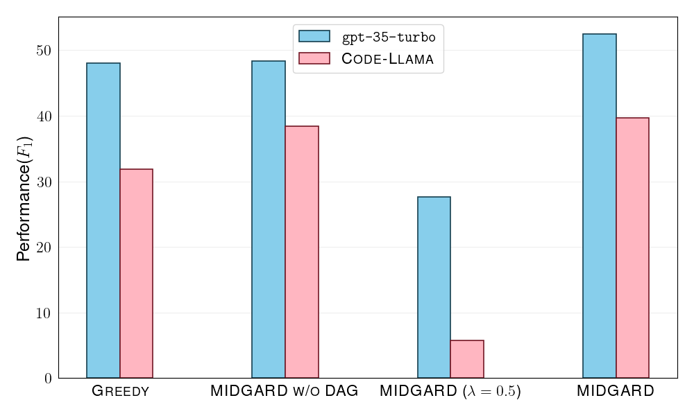
To compare the performance between different approaches, we use F1-score ($F_{1}$) between the inferred edge set and the ground truth. From Figure 3, we can see that MIDGARD significantly improves the performance over the greedy single-generation based approach. The figure also demonstrates the importance of having DAG constraints.

4.4 Task 4: Semantic Graph Generation

Approach	Kelm				WebNLG				GenWiki
	T-F1($\uparrow$)	G-F1($\uparrow$)	G-BS($\uparrow$)	GED($\downarrow$)	T-F1($\uparrow$)	G-F1($\uparrow$)	G-BS($\uparrow$)	GED($\downarrow$)	T-F1($\uparrow$)	G-F1($\uparrow$)	G-BS($\uparrow$)	GED($\downarrow$)
LLM: gpt-3.5-turbo
Greedy	46.9	22.8	84.0	8.7	29.1	15.0	83.6	10.4	23.7	6.5	82.5	11.9
MIDGARD $(\lambda=0.5)$	47.0	22.0	83.2	8.9	27.8	13.2	82.4	10.7	24.0	7.0	82.4	11.6
MIDGARD	47.4	22.8	83.5	8.8	29.3	15.0	83.7	10.4	24.3	7.2	83.4	11.5
LLM: Code-Llama
Greedy	37.9	20.0	63.2	14.1	24.8	6.0	66.4	14.2	12.1	2.0	53.6	17.6
MIDGARD $(\lambda=0.5)$	8.8	4.0	45.0	19.8	23.0	6.0	67.3	14.6	7.1	2.0	54.9	18.2
MIDGARD	37.9	12.0	67.7	13.5	26.5	6.0	77.7	12.2	9.7	4.0	58.7	17.3

Table 4: Results for Semantic Graph Generation. In each of our method variants, we did not apply Dag constraints, as they are not necessary for this task unlike the previous experiments.

The goal of this task is to extract the semantic graph from an input natural language text as a list of edges. Each edge in the graph consists of a subject, a property, and the type of property Han et al. (2023). An example of this task is shown in Appendix D.4.

To gauge the efficacy of our model for such a task, we consider following datasets: (1) Kelm Agarwal et al. (2021), (2) WebNLG Gardent et al. (2017) and (3) GenWiki Jin et al. (2020). For more details on these datasets, we request the reader to refer Appendix D.4

We use the following metrics to assess the quantitative performance as suggested by Han et al. (2023): (1) Triple-Match F₁ (T-F₁) finds the macro-averaged F₁ between the edge triples present in the inference and the ground truth graph edge triples. (2) Graph Match F₁ (G-F₁) measures the performance as the number of graphs which exactly matches the ground truth graph in terms of F₁ score. Finally, as defined in the §4.2, we also use (3) G-BERTScore (G-BS) Zhang et al. (2019) and (4) Graph Edit Distance (GED).

From the Table 7, we can observe that while our approach outperforms or achieves competitive performance compared to the baseline, the performance improvement is not significant for gpt-3.5-turbo. Upon closer examination of the outputs generated using temperature sampling, we have noticed a lack of variability when compared to the structured commonsense reasoning tasks mentioned in the main script. This limited variability hinders the opportunity to improve upon each sample, resulting in a less significant performance boost than expected.

4.5 Further Analyses

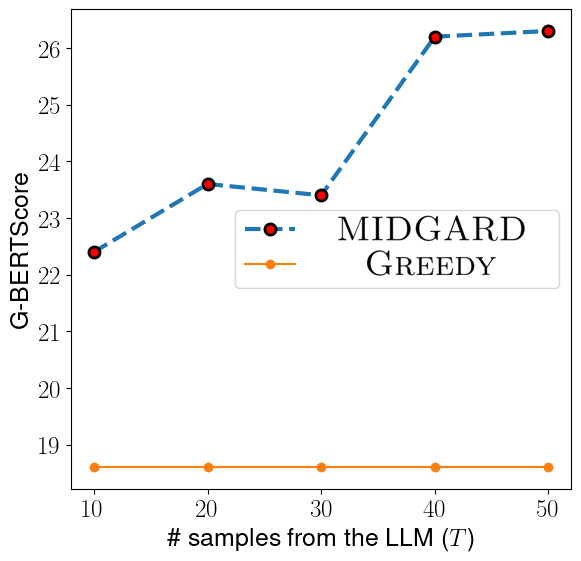
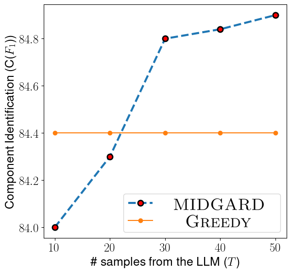
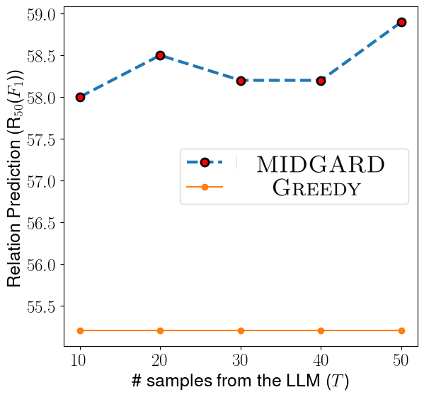
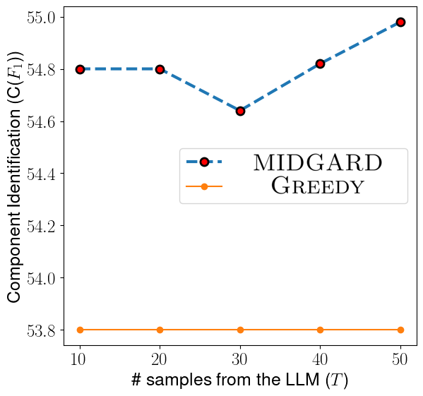
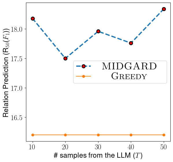
Impact of increasing sample size. To analyze the impact of varying the number of samples generated from the LLM, we evaluate the performance of MIDGARD on the argument structure extraction task as it would allow us to examine the trend on both node identification and edge prediction. We only show the analysis for the Essays dataset from the argument structure extraction task due to limited space. Please refer to the appendix for additional plots and similar analysis.

(a) Component Identification

(b) Relation Prediction

Figure 4: Performance of MIDGARD in comparison with Greedy on Essays when the number of samples from the LLM is varied. Results averaged over $5$ different random seeds.

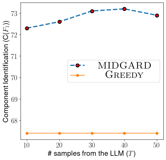
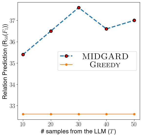
From Fig. 4(a) and Fig. 4(b), we see that the performance increases only marginally emphasizing that returns diminish with increasing the number of samples. Similar trend is observed for other datasets belonging to the same task (refer Appendix E.2). However, for Explagraphs, we observe that the performance steadily increases with the number of samples indicating that having more and diverse explanation graphs is helpful towards improving the final aggregated structure as shown in Figure 5.

Figure 5: Performance of MIDGARD in comparison with Greedy on Explagraphs.

Bin	# Samples	Avg. # Nodes	Avg. # Edges	Avg. Degree	Greedy		MIDGARD
					C	R50	C	R50
Essays
$[5,10)$	3	8.0	7.0	0.88	64.7	23.8	64.7	36.2
$[10,15)$	28	11.2	10.2	0.91	66.2	33.5	70.2	34.8
$[15,20)$	33	15.6	14.6	0.94	68.5	32.5	73.0	36.4
$[20,25)$	14	20.6	19.6	0.95	65.7	32.0	75.5	35.5
$[25,30)$	2	26.0	25.0	0.96	58.3	36.1	70.0	31.2
AbstRCT
$[2,4)$	5	2.8	1.4	0.47	79.4	58.2	77.6	59.6
$[4,6)$	41	4.6	2.7	0.58	83.4	59.8	83.5	63.1
$[6,8)$	36	6.5	3.6	0.56	88.6	57.9	87.6	59.9
$[8,10)$	14	8.4	4.0	0.47	83.8	47.0	84.5	48.3
$[10,12)$	3	10.3	7.0	0.68	70.1	39.6	68.5	50.5
CDCP
$[2,7)$	96	3.9	1.2	0.26	52.1	20.2	52.4	22.3
$[7,12)$	33	8.3	3.2	0.39	56.0	21.7	56.9	23.8
$[12,17)$	13	13.9	3.9	0.27	55.7	8.1	54.9	11.5
$[17,22)$	3	19.0	7.7	0.40	59.7	10.4	64.4	7.7
$[22,27)$	2	23.0	4.5	0.20	52.6	1.1	55.8	1.0

Table 5: Component and Relation identification performance for Greedy and MIDGARD for different graph complexities when gpt-3.5-turbo is used. The results are averaged for $5$ seeds.

Efficacy of MIDGARD for different graph complexities. We compare the performance between MIDGARD and the Greedy approach on argument structure extraction across various graph complexities. We specifically select argument structure extraction for this analysis because it enables us to evaluate the influence of graph complexity on both node and edge identification performance.

In this analysis, we bin the graphs based on the number of nodes and compute the average complexity metrics such as number of nodes and edges and degree for the graphs belonging to each bin. The higher these metrics are, the more complex the corresponding graph is. For each method, we employ gpt-3.5-turbo for generating samples. We observe that our approach provided consistent improvements across different complexities as shown in Table 5.

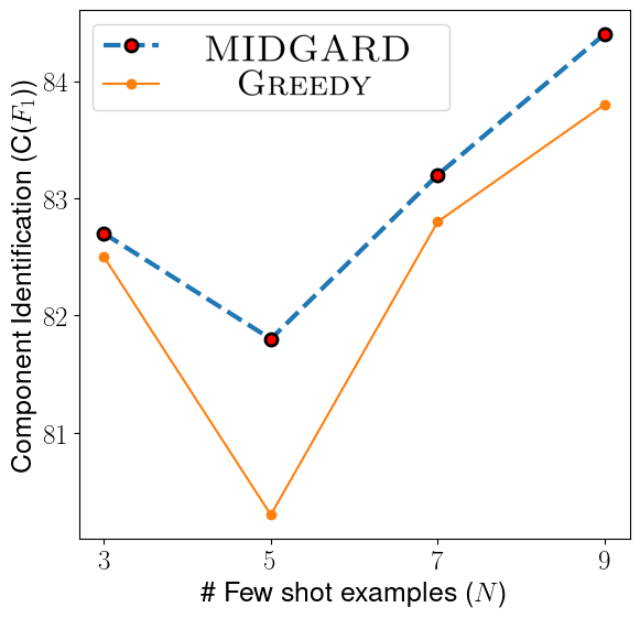
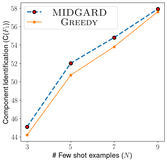
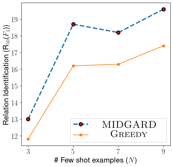
Additional analysis. The impact of varying the number of few-shot examples on argument structure extraction performance for Greedy and MIDGARD is provided in Appendix E.3. MIDGARD consistently improves the performance across different number of few-shot examples. We compare our method and Greedy against a popular decoding technique called Nucleus Sampling Holtzman et al. (2020) in the Appendix E.4 and find that it results in poorer performance. We demonstrate that our approach works with gpt-4 for the Essays dataset in Appendix E.5. In Appendix E.6, we assess the impact of varying the hyperparameters $\{\lambda_{1},\lambda_{2}\}$ on the final performance and compare it with that of automatically estimated hyperparameters (refer Appendix C.3). Figure 15 shows that while our automatic hyperparameter search reaches near optimal performance for component identification, there is a scope for improvement in relation prediction.

5 Related Works

Sampling based approaches using LLMs. A common strategy to address many NLP and commonsense reasoning tasks involves sampling multiple solution trajectories LLMs and employing either a post-hoc strategy Fu et al. (2023); Liu et al. (2023); Wang et al. (2023a) or a trained reranker for sample selection Cobbe et al. (2021); Li et al. (2023); Ni et al. (2023). However, post-hoc approaches relying on LLM evaluation can be prone to position bias Wang et al. (2023a); Zheng et al. (2023) and difficulty in judging response correctness Huang et al. (2023); Gou et al. (2023). Training-based sampling requires additional labeled data for task-specific reranking models. The self-consistency framework is limited to problems with scalar answer spaces due to its reliance on majority voting Ling et al. (2017); Clark et al. (2018); Cobbe et al. (2021); Patel et al. (2021); Geva et al. (2021). Moreover, existing approaches lack integration of information from different samples, potentially leading to suboptimal solutions. In contrast, our MDL-based formulation assimilates relevant information from diverse structured responses without fine-tuning. By examining consistent properties across samples, we construct an aggregate graph that leverages the strengths of each sample.

LLMs for commonsense reasoning. LLMs have been applied to various domains, including arithmetic reasoning He-Yueya et al. (2023), generation of mathematical proofs Welleck et al. (2022), symbolic reasoning Wei et al. (2022), and logical reasoning Srivastava et al. (2022). While prompting strategies Wei et al. (2022); Zhou et al. (2022); Yao et al. (2022); Wang et al. (2023b); Yao et al. (2023); Madaan et al. (2023) have been proposed to improve performance across these tasks, adapting them to structured commonsense reasoning, which involves generating complex graph structures, presents unique challenges Madaan et al. (2022). Additionally, tasks within structured commonsense reasoning often require adherence to specific constraints Saha et al. (2021); Sakaguchi et al. (2021), such as directed acyclicity, which are difficult to ensure solely through existing strategies. Our approach is independent of the prompting methodology and allows for flexible incorporation of task-specific constraints during inference.

6 Conclusion

We proposed a novel approach for enhancing the performance of structured reasoning problems which involve generating task-specific graphs. Taking inspiration from self-consistency, we sample multiple graphs from the LLM and devise a mechanism to construct aggregated graph. Through rigorous experimentation, we have demonstrated the effectiveness of our approach across various structured commonsense reasoning tasks.

Limitations

• Due to our approach’s reliance on generating multiple samples, it can be computationally demanding and may require a significant amount of time, particularly without batched inference. As a result, practitioners using enterprise LLMs may incur substantially higher costs compared to methods that involve single generation. This factor makes our approach less desirable in situations where there are constraints on compute budget or limited machinery resources.

• For datasets consisting of graphs with a small number of nodes and edges, applying ILP does not result in significant computational overhead. However, it is important to acknowledge that the time complexity of ILP solvers grows exponentially with the complexity of the problem. Therefore, modifications are necessary when applying our approach to settings with a large number of edges and nodes. Additionally, as the graph size increases, it becomes increasingly challenging to utilize LLMs effectively in generating the graph structure. The limited context length of the LLMs poses a challenge for applying them to commonsense reasoning tasks involving larger graphs. This limitation arises from the difficulty of accommodating multiple in-context learning examples within the given context length.

Ethics Statement

While our methodology attempts to derive structured representations from the input data only, due to the issue of hallucination, the LLMs are not immune to generating biased, insensitive or untruthful content. Hence, we urge practitioners and researchers to exercise caution when applying our framework, especially for sensitive applications like politics, finance, and healthcare.

Appendix A Minimum Description Length Principle

The principle of Minimum Description Length (MDL) aims to find a model that can efficiently represent a dataset using the fewest bits, while also minimizing model complexity. In simpler terms, it seeks to find the least complex model that can effectively capture the regularities in a given dataset using the least amount of bits. Let’s denote the dataset that needs to be represented as $\mathcal{D}$, and the model as $H\in\mathcal{H}$. We represent the description length of $\mathcal{D}$ when using $H$ as $L(\mathcal{D}|H)$, which quantifies the number of bits required to describe $\mathcal{D}$ using $H$. Additionally, let’s define $L(H)$ as the complexity of the model. Formally, MDL aims to find the optimal solution for:

$$H^{*}=\arg\min_{H\in\mathcal{H}}L(\mathcal{D}|H)+L(H)$$ (10)

To explain what each of these terms corresponds to in our approach, let’s consider the objective for graphs that do not have singleton nodes in §3.3, while adhering to the constraint that the sought-after graph is a Directed Acyclic Graph (DAG). In this scenario, the hypothesis family $\mathcal{H}$ encompasses all graphs with nodes and edges in $\mathbf{N}$ and $\mathbf{E}$, respectively. The dataset in our case consists of samples derived from the LLM, which can be denoted as $\mathcal{D}=\{\mathcal{G}^{\prime}\}_{i=1}^{T}$. The formulation of $L(\mathcal{D}|H)$ takes the form of Equation 1. Lastly, we define the complexity of the model $L(H)$ as $0$ if $H$ is a DAG, and $\infty$ otherwise.

Appendix B Restricting hypothesis selection to DAGs

To describe the strategy to restrict hypothesis selection to DAGs, we can express $\mathbf{E}$ as the set $\{(n_{1},n_{2})\,|\,n_{1}\in\mathbf{N},n_{2}\in\mathbf{N}\}$ where $n_{1}$($n_{2}$) represents the head (tail) of the edge $(n_{1},n_{2})$. We formulate objective 7 as an Integer Linear Programming (ILP) problem by introducing one more binary variable $b_{e}$ for each edge $e\in\mathbf{E}$. $b_{e}$ is set as $1$ if there exists a path from the head of $e$ to its tail. Under ILP, we optimize 7 subject to the following constraints:

$$\begin{aligned} \mathllap{\forall e\in\mathbf{E}}&:x_{e}-b_{e}\leq 0\\ \end{aligned}$$ (11)

$$\begin{aligned} \mathllap{\forall n_{1},n_{2},n_{3}\in\mathbf{N}}&:b_{(n_{1},n_{3})}-b_{(n_{1},n_{2})}\\ &-b_{(n_{2},n_{3})}\geq-1\\ \end{aligned}$$ (12)

$$\begin{aligned} \mathllap{\forall n\in\mathbf{N}}&:b_{(n,n)}=0\\ \end{aligned}$$ (13)

The constraint represented by LABEL:eqn:direct_edge ensures that there is a path between two nodes if they are directly connected by an edge. LABEL:eqn:transitivity enforces the requirement that a path must exist between two nodes if there is a path from the first node to a third node, and this third node is connected to the second node. Lastly, LABEL:eqn:no_cycle prevents any cycles from occurring in the graph.

Appendix C Implementation Details

In this section, we begin by explaining the construction of $\mathbf{N}$ and $\mathbf{E}$ based on the samples $\{\mathcal{G^{\prime}}_{i}\}_{i=1}^{T}\sim\mathbb{P}_{c}\left(\cdot,\mathcal{T}\right)$. Thereafter, we describe how the hyperparameters $\lambda_{1}$ and $\lambda_{2}$ are set.

C.1 Constructing $\mathbf{N}$ and $\mathbf{E}$

To build $\mathbf{N}$, we iterate through the samples $\{\mathcal{G}^{\prime}_{i}\}_{i=1}^{T}$. It is important to note that each node in $\mathcal{G}^{\prime}_{i}$ consists of two primary properties: content and type. For example, in argument structure extraction Stab and Gurevych (2017), a node represents an argumentative component with content indicating its value and type indicating its category, such as premise/claim.

When we are iterating over the nodes in $\bigcup_{i=1}^{T}N(\mathcal{G^{\prime}}_{i})$, we have two choices: append it as a new node or merge it with some other node present in $\mathbf{N}$. To keep track of the historical merging of nodes with $n\in\mathbf{N}$, we maintain two lists: content_list and type_list. These lists store the content and type properties of the nodes that have been merged with $n$ over time, respectively. Moreover, content_list property can also be used to decide whether a new node has to merged. If the Jaccard similarity between the set of tokens in the content of the new node and the set of tokens in an element of content_list for $n$ exceeds a pre-defined threshold, we add the content and type properties of the new node to the respective lists associated with $n$. Finally, the sentence from the content_list with the highest Jaccard similarity to the rest of the elements, and the mode of the type_list of $n$, are chosen as its content and type, respectively. The number of samples containing $n$ is simply the length of its content_list which can be used to estimate $\mathbb{P}_{\mathcal{G}^{\prime}}(n)$.

Similarly, we initialize $\mathbf{E}=\{(n_{1},n_{2})\,|\,n_{1},n_{2}\in\mathbf{N}\}$. Just like before, each edge in any sample is linked to a specific type property that characterizes the attribute associated with it. For example, in argument structure extraction, the type of an edge can be defined as attack or support, indicating the relationship between the head and the tail of the edge. As before, we associate type_list property to each $e\in\mathbf{E}$, which records the observed type property for that edge across all the samples it appears in. Finally, the type of each edge is the mode of its type_list property.

C.2 Constructing Optimal Aggregate Graph

After constructing $\mathbf{N}$ and $\mathbf{E}$, we apply an appropriate formulation of the objective in §3 to get the optimal values of $x_{e}(\forall e\in\mathbf{E})$ and $y_{n}(\forall n\in\mathbf{N})$. Thereafter, we return the hypothesis $\mathbf{G}$ where $N(\mathcal{G})=\{n\,|\,y_{n}=1,n\in\mathbf{N}\}$ and $E(\mathcal{G})=\{e\,|\,x_{e}=1,e\in\mathbf{E}\}$. If singleton nodes are absent, we only retain nodes that are present as a head or tail in $E(\mathcal{G})$.

C.3 Hyperparameter selection

To automatically select appropriate values for the hyperparameters $\{\lambda_{1},\lambda_{2}\}$, we utilize k-fold cross validation using the few-shot examples. In each fold, the held-out set comprises a single data point, while the training set consists of $k-1$ data points.

C.4 Generating graphs from LLMs

For each dataset, the graph structure is encoded as a programming script following the guidelines of CoCoGen (refer appendix D.1). Multiple samples are generated from the LLM using a temperature of $0.9$. To address the randomness in sampling few-shot examples and temperature sampling, we use 5 different random seeds.

Once the LLM generates the graph as a programming script, we obtain the corresponding graph $\mathcal{G}^{\prime}$, a parser is needed to process this output. During sampling from the LLM, we assume that the textual response can be parsed into the corresponding graph using a task-specific rule-based parser.

Appendix D Additional information on considered tasks

D.1 Task 1: Argument Structure Extraction - Additional Information on task, prompt design and datasets

In this section, we show an example of this task and describe the prompt used for our experiments. The example for demonstrating this task is taken from one of the paragraphs in a datapoint belonging to the Essays dataset.

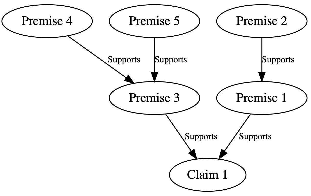
First, [cloning will be beneficial for many people who are in need of organ transplants]${}_{\textrm{Claim 1}}$. [Cloned organs will match perfectly to the blood group and tissue of patients]${}_{\textrm{Premise 1}}$ since [they can be raised from cloned stem cells of the patients]${}_{\textrm{Premise 2}}$. In addition, [it shortens the healing process]${}_{\textrm{Premise 3}}$. Usually [it is very rare to find an appropriate organ donor]${}_{\textrm{Premise 4}}$ and [by using cloning in order to raise required organs the waiting time can be shortened tremendously]${}_{\textrm{Premise 5}}$.

Table 6: An example text with annotated argumentative components.

Figure 6: Relations between the argumentative components of the example introduced in §D.1

.

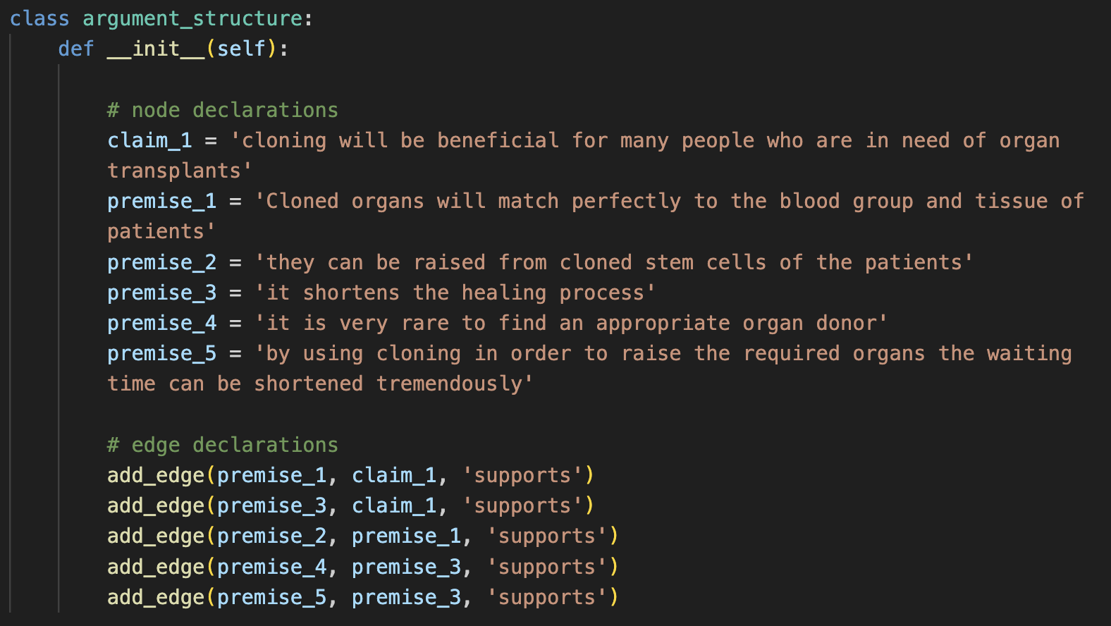
The example in Table 6 shows the different argumentative components in a text along with their categories. The objective of argument structure extraction entails not only the identification of different argumentative components but also the prediction of support or attack relations between them. The argumentative relations between the components is shown in Figure 6. The equivalent programming script representation of the aforementioned structure is shown in Figure 7.

Now, we provide some information on the datasets used to evaluate various approaches. We considered the following 3 datasets. (1) Essays Stab and Gurevych (2017) that consists of essays obtained from essaysforum.com. Each argumentative component within the essays is labeled at a sub-sentence level as either a premise, claim, or major claim. The relationships between these components are labeled as either attack or support. Test split consisting of $80$ datapoints is used for evaluation. We randomly select $7$ data points from the training split in the few-shot prompt. (2) AbstRCT Mayer et al. (2020) is constructed by annotating the argumentative structure in the abstracts of PubMed articles on Randomized Controlled Trial of diseases. For our few-shot set, we randomly choose $11$ data points from the training split. The dataset includes three test splits: two from homogeneous data sources and one constructed by collecting data points from various sources, including the homogeneous ones. We focus on evaluating the performance of our model on the test split curated from various sources, which consists of $100$ data points. (3) CDCP Park and Cardie (2018) is obtained from a public forum where argumentative texts regarding proposed rules on Consumer Debt Collection Practices (CDCP) are annotated with argumentative components and the corresponding support relations. From the training set, we randomly select $7$ data points as our few-shot prompt. We then assess the performance of our model on the test split, which consists of $150$ data points.

Figure 7: Programming script prompt used for argument structure extraction

D.2 Task 2: Explanation Graph Generation: Additional information on prompt design and datasets

As we are focusing on the task of generating the commonsense structure, we assume that the stance is provided and prompt the model to generate the structure only as done in Madaan et al. (2022). We use the same prompt scheme as employed by CoCoGen in representing a graph as a programming script by directly adopting their implementation.

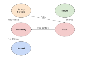
In this implementation, $30$ few-shot instances were used to prompt the LLM and the approach was evaluated over the development split consisting of $396$ datapoints. An example explanation task for this task is shown in Figure 8 for the following belief, argument and stance:

Belief: Factory farming should not be banned.
Argument: Factory farming feeds millions.
Stance: Support

Figure 8: Explanation graph for the example shown in the Appendix D.2.

D.3 Task 3: Script Planning: Additional information on task, prompt design and datasets

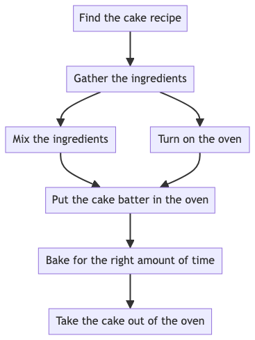
The input in Proscript Sakaguchi et al. (2021) specifies the high-level goal to be achieved and the intermediate steps required to achieve the goal. The task involves inferring a sequence of dependency relationships among these steps, where each directed arrow indicates that the step at the arrow’s head must be executed before the step at the tail. We utilize this dataset to evaluate the ability of various algorithms to automatically determine the order of operations needed to achieve the specified goal. We used $15$ few-shot instances for prompting and assessed the performance of various approaches over $100$ samples from the development dataset. An example of this datapoint is shown in Figure 9.

Figure 9: Script Planning for the goal "bake a cake". The steps shown in the figure are also provided as part of the input. The model has to predict directed relations between the steps that captures the temporal relations among them.

D.4 Task 4: Semantic Graph Generation: Additional information on task, prompt design and datasets

Input Text: While pop rock can trace its stylistic roots back to rock music, Reggae music evolved out of different musical genre, known as ska. Interestingly, the Train song, Mermaid, belongs to the genre of pop rock, but is also considered to be of the reggae genre as well

Semantic Structure: ("Mermaid Train song", "genre", "Pop rock"), ("Mermaid Train song", "genre", "Reggae"), ("Pop rock", "stylistic Origin", "Rock music"), ("Reggae", "stylistic Origin", "Ska")

Table 7: An example for Semantic Graph Generation.

The goal of this task is to extract the semantic graph from an input graph, which is represented as a list of edges. Each edge in the graph consists of a subject, a property, and the type of property. Han et al. (2023). An example of this task is shown in 7.

To gauge the efficacy of our model for such a task, we consider following datasets: (1) Kelm Agarwal et al. (2021): This is a large scale synthetic dataset where each datapoint consists of a sentence in natural language and the corresponding semantic structure in the form of linearized Knowledge Graph (KG). Most of the graphs in this dataset contains at most $6$ edges. (2) WebNLG Gardent et al. (2017): The datapoints in this dataset were curated by sampling triples from the DBpedia Auer et al. (2007). The sentences describing their respective graphs were crafted using a wide range of lexicalization patterns. (3) GenWiki Jin et al. (2020): Unlike previous datasets, this one does not provide paired datapoints that map a natural language sentence to its corresponding semantic graph representation. However, a technique formulated by Han et al. (2023) allows for the synthesis of pairwise annotated datasets, which we utilize in our assessments.

Appendix E Additional Analysis

E.1 Precision / Recall analysis for Argument structure extraction

Approach	Essays				AbstRCT				CDCP
	C(P)	C(R)	R50(P)	R50(R)	C(P)	C(R)	R50(P)	R50(R)	C(P)	C(R)	R50(P)	R50(R)
Greedy	77.7	59.6	37.4	28.9	86.9	81.9	50.1	61.4	55.0	52.6	13.4	21.0
MIDGARD	74.0	70.7	40.5	31.9	86.0	82.1	53.7	63.3	55.9	53.7	14.4	25.9

Table 8: Component and Relation Identification precision and recall for MIDGARD and Greedy. P and R within the parentheses represent precision and recall respectively.

In order to empirically demonstrate the effectiveness of our algorithm in reducing errors, we compute the precision and recall in component and relation identification for argument structure extraction. This analysis not only allows us to assess the efficacy of our approach in filtering out false properties, but also in capturing genuine properties from multiple samples that would have otherwise been overlooked if only a single sample was relied upon. Instead of using the F₁-scores of the metrics C and R₅₀ defined in §4.1, we compute the precision and recall of these metrics under same definition. Specifically, the precision and recall along component identification is denoted by C(P) and C(R). A consistent notation is used for relation identification as well.

From the Table 8, MIDGARD consistently improves the recall for component and relation identification across all datasets as it relies on multiple samples to formulate the final hypothesis, effectively addressing the issue of omitting true properties that would arise if relied on a single sample alone. Moreover, utilizing the consistencies among the samples leads to improved precision for relation identification, thereby helping reduce the number of spurious samples. While the precision for component identification is slightly impacted, adjusting the value of $\lambda_{1}$ allows us to achieve higher precision at the cost of slightly reduced recall.

E.2 Impact of increasing the number of samples for other argument structure extraction tasks

(a) Component Identification

(b) Relation Prediction

Figure 10: Performance of MIDGARD in comparison with Greedy for the AbstRCT Dataset when the number of samples from the LLM is varied. Results averaged over $5$ different random seeds.

(a) Component Identification

(b) Relation Prediction

Figure 11: Performance of MIDGARD in comparison with Greedy for the CDCP Dataset when the number of samples from the LLM is varied. Results averaged over $5$ different random seeds.

E.3 Impact of changing the number of few-shot examples for argument structure extraction

(a) Component Identification

(b) Relation Prediction

Figure 12: Performance of MIDGARD in comparison with Greedy for the Essays Dataset when the number of few shot examples ($N$) is varied. Results averaged over $5$ different random seeds.

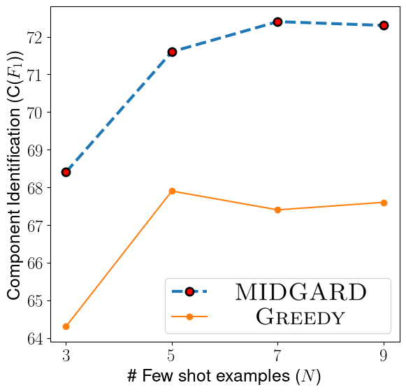
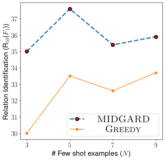
We assess the effectiveness of our approach for different numbers of few-shot instances ($N\in\{3,5,7,9\}$) in the context of argument structure extraction when $10$ samples are used from the LLM. As shown in Figure 12, MIDGARD consistently enhances the performance of Greedy approach across different numbers of few shot examples. The plots for AbstRCT and CDCP are shown in Figure 13 and Figure 14 respectively.

(a) Component Identification

(b) Relation Prediction

Figure 13: Performance of MIDGARD in comparison with Greedy for the AbstRCT Dataset when the number of few shot examples ($N$) is varied. Results averaged over $5$ different random seeds.

(a) Component Identification

(b) Relation Prediction

Figure 14: Performance of MIDGARD in comparison with Greedy for the CDCP Dataset when the number of few shot examples ($N$) is varied. Results averaged over $5$ different random seeds.

E.4 Comparison with Nucleus Sampling

While our evaluations considered Greedy decoding, we also compare against the Nucleus decoding Holtzman et al. (2020), a popular technique to combat neural text degeneration, for the task of argument structure extraction in Essays. As shown in the Table 9, the application of Nucleus decoding degrades the performance significantly for both the considered LLMs.

Approach	C	R100	R50
LLM: gpt-35-turbo
Greedy	67.4	21.5	32.6
Nucleus	64.1	19.2	31.2
MIDGARD	72.3	23.5	35.4
LLM: Code-Llama
Greedy	56.3	9.3	21.4
Nucleus	48.0	6.7	16.7
MIDGARD	60.3	11.0	24.5

Table 9: Comparison of different approaches on gpt-35-turbo and Code-LLAMA models.

E.5 Performance for gpt-4

Due to the prohibitive expense associated with gpt-4, we were limited in assessing its performance across all tasks. However, we have successfully evaluated its capabilities on the Argument Structure Extraction task using a selective subset of $20$ data points from the Essays Dataset. This specific evaluation thoroughly addresses both the identification of components (node evaluation) and the prediction of relations (edge evaluation), offering a more comprehensive analysis compared to other tasks. For the Essays dataset, which includes $80$ test data points, the estimated cost for GPT-4 analysis across 5 random instances of few-shot training examples could exceed $\$1000$. Given that other argument structure extraction datasets comprise over 80 test points, the expected inference costs would significantly increase. The results for the Essays dataset are tabulated in Table 10.

Approach	C	R100	R50
LLM: gpt-4
Greedy	77.1	30.7	40.9
MIDGARD	78.1	32.9	42.8

Table 10: Comparison of different approaches implemented on gpt-4 for Essays Dataset

E.6 Hyperparameters

In this experiment, we vary $\lambda_{1},\lambda_{2}\in\{0.0,0.1,0.2,\dots,1.0\}$ and compute the performance of component identification and relation prediction on Essays, and compare with that of hyperparameters automatically estimated (see Appendix C.3 for more details). Specifically, when varying $\lambda_{1}$, we set $\lambda_{2}$ to 1 in order to include all nodes in the hypothesis and focus solely on studying the influence of $\lambda_{1}$ on relation prediction. An analogous step is repeated to study the influence of $\lambda_{2}$ on component identification.

(a) Component Identification

(b) Relation Prediction

Figure 15: Assessing the performance of our algorithm for different values of $\{\lambda_{1},\lambda_{2}\}$ and comparing it with that of automatically estimated hyperparameters. Results averaged over $5$ different random seeds.

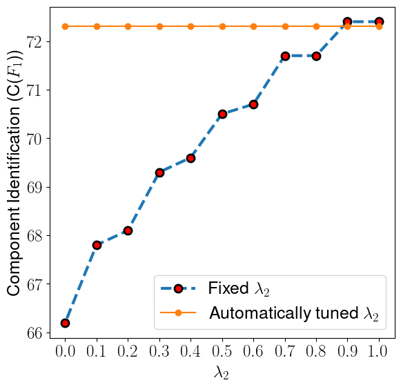
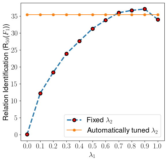
In Figure 15, we observe that the automatically estimated hyperparameter ($\lambda_{2}$) for component identification is near optimal performance. However, there is room for improvement in selecting $\lambda_{1}$. Additionally, we find that the optimal values for both hyperparameters are above $0.5$, suggesting that the description length of insertion is greater than that of deletion, as discussed in Section 3.2.

Appendix F Intuitive explanation for having unequal description lengths with addition versus deletion

To define a single deletion, it requires $\propto\log_{2}(|E(\mathcal{G})|)$ to specify the edge to be deleted from $\mathcal{G}$. On the other hand, to describe the edge to be added one needs to spend $\propto\log_{2}(|\mathbf{E}|)$ bits. Clearly, $\log_{2}(|\mathbf{E}|)\geq\log_{2}(|E(\mathcal{G})|)$ as $\mathbf{E}\supseteq E(\mathcal{G})$.

References

- Agarwal et al. (2021) Oshin Agarwal, Heming Ge, Siamak Shakeri, and Rami Al-Rfou. 2021. Knowledge graph based synthetic corpus generation for knowledge-enhanced language model pre-training. In Proceedings of the 2021 Conference of the North American Chapter of the Association for Computational Linguistics: Human Language Technologies, pages 3554–3565, Online. Association for Computational Linguistics.
- Auer et al. (2007) Sören Auer, Christian Bizer, Georgi Kobilarov, Jens Lehmann, Richard Cyganiak, and Zachary Ives. 2007. Dbpedia: A nucleus for a web of open data. In The Semantic Web, pages 722–735, Berlin, Heidelberg. Springer Berlin Heidelberg.
- Brown et al. (2020) Tom Brown, Benjamin Mann, Nick Ryder, Melanie Subbiah, Jared D Kaplan, Prafulla Dhariwal, Arvind Neelakantan, Pranav Shyam, Girish Sastry, Amanda Askell, et al. 2020. Language models are few-shot learners. Advances in neural information processing systems, 33:1877–1901.
- Bruni et al. (2022) Vittoria Bruni, Maria Lucia Cardinali, and Domenico Vitulano. 2022. A short review on minimum description length: An application to dimension reduction in pca. Entropy, 24(2):269.
- Chen et al. (2021) Mark Chen, Jerry Tworek, Heewoo Jun, Qiming Yuan, Henrique Ponde de Oliveira Pinto, Jared Kaplan, Harri Edwards, Yuri Burda, Nicholas Joseph, Greg Brockman, et al. 2021. Evaluating large language models trained on code. arXiv preprint arXiv:2107.03374.
- Chowdhery et al. (2022) Aakanksha Chowdhery, Sharan Narang, Jacob Devlin, Maarten Bosma, Gaurav Mishra, Adam Roberts, Paul Barham, Hyung Won Chung, Charles Sutton, Sebastian Gehrmann, Parker Schuh, Kensen Shi, Sasha Tsvyashchenko, Joshua Maynez, Abhishek Rao, Parker Barnes, Yi Tay, Noam Shazeer, Vinodkumar Prabhakaran, Emily Reif, Nan Du, Ben Hutchinson, Reiner Pope, James Bradbury, Jacob Austin, Michael Isard, Guy Gur-Ari, Pengcheng Yin, Toju Duke, Anselm Levskaya, Sanjay Ghemawat, Sunipa Dev, Henryk Michalewski, Xavier Garcia, Vedant Misra, Kevin Robinson, Liam Fedus, Denny Zhou, Daphne Ippolito, David Luan, Hyeontaek Lim, Barret Zoph, Alexander Spiridonov, Ryan Sepassi, David Dohan, Shivani Agrawal, Mark Omernick, Andrew M. Dai, Thanumalayan Sankaranarayana Pillai, Marie Pellat, Aitor Lewkowycz, Erica Moreira, Rewon Child, Oleksandr Polozov, Katherine Lee, Zongwei Zhou, Xuezhi Wang, Brennan Saeta, Mark Diaz, Orhan Firat, Michele Catasta, Jason Wei, Kathy Meier-Hellstern, Douglas Eck, Jeff Dean, Slav Petrov, and Noah Fiedel. 2022. Palm: Scaling language modeling with pathways.
- Clark et al. (2018) Peter Clark, Isaac Cowhey, Oren Etzioni, Tushar Khot, Ashish Sabharwal, Carissa Schoenick, and Oyvind Tafjord. 2018. Think you have solved question answering? try arc, the ai2 reasoning challenge. arXiv preprint arXiv:1803.05457.
- Cobbe et al. (2021) Karl Cobbe, Vineet Kosaraju, Mohammad Bavarian, Mark Chen, Heewoo Jun, Lukasz Kaiser, Matthias Plappert, Jerry Tworek, Jacob Hilton, Reiichiro Nakano, et al. 2021. Training verifiers to solve math word problems. arXiv preprint arXiv:2110.14168.
- Fu et al. (2023) Jinlan Fu, See-Kiong Ng, Zhengbao Jiang, and Pengfei Liu. 2023. Gptscore: Evaluate as you desire. arXiv preprint arXiv:2302.04166.
- Gardent et al. (2017) Claire Gardent, Anastasia Shimorina, Shashi Narayan, and Laura Perez-Beltrachini. 2017. The WebNLG challenge: Generating text from RDF data. In Proceedings of the 10th International Conference on Natural Language Generation, pages 124–133, Santiago de Compostela, Spain. Association for Computational Linguistics.
- Geva et al. (2021) Mor Geva, Daniel Khashabi, Elad Segal, Tushar Khot, Dan Roth, and Jonathan Berant. 2021. Did aristotle use a laptop? a question answering benchmark with implicit reasoning strategies. Transactions of the Association for Computational Linguistics, 9:346–361.
- Gou et al. (2023) Zhibin Gou, Zhihong Shao, Yeyun Gong, Yelong Shen, Yujiu Yang, Nan Duan, and Weizhu Chen. 2023. Critic: Large language models can self-correct with tool-interactive critiquing. arXiv preprint arXiv:2305.11738.
- Grünwald (2005) Peter Grünwald. 2005. Minimum description length tutorial. Advances in minimum description length: Theory and applications, 5:1–80.
- Han et al. (2023) Jiuzhou Han, Nigel Collier, Wray Buntine, and Ehsan Shareghi. 2023. Pive: Prompting with iterative verification improving graph-based generative capability of llms. arXiv preprint arXiv:2305.12392.
- He-Yueya et al. (2023) Joy He-Yueya, Gabriel Poesia, Rose E Wang, and Noah D Goodman. 2023. Solving math word problems by combining language models with symbolic solvers. arXiv preprint arXiv:2304.09102.
- Hoffmann et al. (2022) Jordan Hoffmann, Sebastian Borgeaud, Arthur Mensch, Elena Buchatskaya, Trevor Cai, Eliza Rutherford, Diego de Las Casas, Lisa Anne Hendricks, Johannes Welbl, Aidan Clark, Tom Hennigan, Eric Noland, Katie Millican, George van den Driessche, Bogdan Damoc, Aurelia Guy, Simon Osindero, Karen Simonyan, Erich Elsen, Jack W. Rae, Oriol Vinyals, and Laurent Sifre. 2022. Training compute-optimal large language models.
- Holtzman et al. (2020) Ari Holtzman, Jan Buys, Li Du, Maxwell Forbes, and Yejin Choi. 2020. The curious case of neural text degeneration. In International Conference on Learning Representations.
- Hua et al. (2019) Xinyu Hua, Mitko Nikolov, Nikhil Badugu, and Lu Wang. 2019. Argument mining for understanding peer reviews. In Proceedings of the 2019 Conference of the North American Chapter of the Association for Computational Linguistics: Human Language Technologies, Volume 1 (Long and Short Papers), pages 2131–2137, Minneapolis, Minnesota. Association for Computational Linguistics.
- Hua and Wang (2022) Xinyu Hua and Lu Wang. 2022. Efficient argument structure extraction with transfer learning and active learning. In Findings of the Association for Computational Linguistics: ACL 2022, pages 423–437, Dublin, Ireland. Association for Computational Linguistics.
- Huang et al. (2023) Jie Huang, Xinyun Chen, Swaroop Mishra, Huaixiu Steven Zheng, Adams Wei Yu, Xinying Song, and Denny Zhou. 2023. Large language models cannot self-correct reasoning yet. arXiv preprint arXiv:2310.01798.
- Jin et al. (2020) Zhijing Jin, Qipeng Guo, Xipeng Qiu, and Zheng Zhang. 2020. GenWiki: A dataset of 1.3 million content-sharing text and graphs for unsupervised graph-to-text generation. In Proceedings of the 28th International Conference on Computational Linguistics, pages 2398–2409, Barcelona, Spain (Online). International Committee on Computational Linguistics.
- Lam and Bacchus (1993) Wai Lam and Fahiem Bacchus. 1993. Using causal information and local measures to learn bayesian networks. In Uncertainty in Artificial Intelligence, pages 243–250. Elsevier.
- Lam and Bacchus (1994) Wai Lam and Fahiem Bacchus. 1994. Using new data to refine a bayesian network. In Uncertainty Proceedings 1994, pages 383–390. Elsevier.
- Li et al. (2023) Yifei Li, Zeqi Lin, Shizhuo Zhang, Qiang Fu, Bei Chen, Jian-Guang Lou, and Weizhu Chen. 2023. Making language models better reasoners with step-aware verifier. In Proceedings of the 61st Annual Meeting of the Association for Computational Linguistics (Volume 1: Long Papers), pages 5315–5333, Toronto, Canada. Association for Computational Linguistics.
- Ling et al. (2017) Wang Ling, Dani Yogatama, Chris Dyer, and Phil Blunsom. 2017. Program induction by rationale generation: Learning to solve and explain algebraic word problems. In Proceedings of the 55th Annual Meeting of the Association for Computational Linguistics (Volume 1: Long Papers), pages 158–167, Vancouver, Canada. Association for Computational Linguistics.
- Liu et al. (2023) Yang Liu, Dan Iter, Yichong Xu, Shuohang Wang, Ruochen Xu, and Chenguang Zhu. 2023. Gpteval: Nlg evaluation using gpt-4 with better human alignment. arXiv preprint arXiv:2303.16634.
- Madaan et al. (2021) Aman Madaan, Dheeraj Rajagopal, Niket Tandon, Yiming Yang, and Eduard Hovy. 2021. Could you give me a hint ? generating inference graphs for defeasible reasoning. In Findings of the Association for Computational Linguistics: ACL-IJCNLP 2021, pages 5138–5147, Online. Association for Computational Linguistics.
- Madaan et al. (2023) Aman Madaan, Niket Tandon, Prakhar Gupta, Skyler Hallinan, Luyu Gao, Sarah Wiegreffe, Uri Alon, Nouha Dziri, Shrimai Prabhumoye, Yiming Yang, et al. 2023. Self-refine: Iterative refinement with self-feedback. arXiv preprint arXiv:2303.17651.
- Madaan and Yang (2021) Aman Madaan and Yiming Yang. 2021. Neural language modeling for contextualized temporal graph generation. In Proceedings of the 2021 Conference of the North American Chapter of the Association for Computational Linguistics: Human Language Technologies, pages 864–881, Online. Association for Computational Linguistics.
- Madaan et al. (2022) Aman Madaan, Shuyan Zhou, Uri Alon, Yiming Yang, and Graham Neubig. 2022. Language models of code are few-shot commonsense learners. In Proceedings of the 2022 Conference on Empirical Methods in Natural Language Processing, pages 1384–1403, Abu Dhabi, United Arab Emirates. Association for Computational Linguistics.
- Mayer et al. (2020) Tobias Mayer, Elena Cabrio, and Serena Villata. 2020. Transformer-based argument mining for healthcare applications. In ECAI 2020, pages 2108–2115. IOS Press.
- Ni et al. (2023) Ansong Ni, Srini Iyer, Dragomir Radev, Veselin Stoyanov, Wen-tau Yih, Sida Wang, and Xi Victoria Lin. 2023. Lever: Learning to verify language-to-code generation with execution. In International Conference on Machine Learning, pages 26106–26128. PMLR.
- Park and Cardie (2018) Joonsuk Park and Claire Cardie. 2018. A corpus of eRulemaking user comments for measuring evaluability of arguments. In Proceedings of the Eleventh International Conference on Language Resources and Evaluation (LREC 2018), Miyazaki, Japan. European Language Resources Association (ELRA).
- Patel et al. (2021) Arkil Patel, Satwik Bhattamishra, and Navin Goyal. 2021. Are NLP models really able to solve simple math word problems? In Proceedings of the 2021 Conference of the North American Chapter of the Association for Computational Linguistics: Human Language Technologies, pages 2080–2094, Online. Association for Computational Linguistics.
- Qiao et al. (2022) Shuofei Qiao, Yixin Ou, Ningyu Zhang, Xiang Chen, Yunzhi Yao, Shumin Deng, Chuanqi Tan, Fei Huang, and Huajun Chen. 2022. Reasoning with language model prompting: A survey. arXiv preprint arXiv:2212.09597.
- Rae et al. (2022) Jack W. Rae, Sebastian Borgeaud, Trevor Cai, Katie Millican, Jordan Hoffmann, Francis Song, John Aslanides, Sarah Henderson, Roman Ring, Susannah Young, Eliza Rutherford, Tom Hennigan, Jacob Menick, Albin Cassirer, Richard Powell, George van den Driessche, Lisa Anne Hendricks, Maribeth Rauh, Po-Sen Huang, Amelia Glaese, Johannes Welbl, Sumanth Dathathri, Saffron Huang, Jonathan Uesato, John Mellor, Irina Higgins, Antonia Creswell, Nat McAleese, Amy Wu, Erich Elsen, Siddhant Jayakumar, Elena Buchatskaya, David Budden, Esme Sutherland, Karen Simonyan, Michela Paganini, Laurent Sifre, Lena Martens, Xiang Lorraine Li, Adhiguna Kuncoro, Aida Nematzadeh, Elena Gribovskaya, Domenic Donato, Angeliki Lazaridou, Arthur Mensch, Jean-Baptiste Lespiau, Maria Tsimpoukelli, Nikolai Grigorev, Doug Fritz, Thibault Sottiaux, Mantas Pajarskas, Toby Pohlen, Zhitao Gong, Daniel Toyama, Cyprien de Masson d’Autume, Yujia Li, Tayfun Terzi, Vladimir Mikulik, Igor Babuschkin, Aidan Clark, Diego de Las Casas, Aurelia Guy, Chris Jones, James Bradbury, Matthew Johnson, Blake Hechtman, Laura Weidinger, Iason Gabriel, William Isaac, Ed Lockhart, Simon Osindero, Laura Rimell, Chris Dyer, Oriol Vinyals, Kareem Ayoub, Jeff Stanway, Lorrayne Bennett, Demis Hassabis, Koray Kavukcuoglu, and Geoffrey Irving. 2022. Scaling language models: Methods, analysis & insights from training gopher.
- Rissanen (1978) J. Rissanen. 1978. Modeling by shortest data description. Automatica, 14(5):465–471.
- Rissanen (2000) Jorma Rissanen. 2000. Mdl denoising. IEEE Transactions on Information Theory, 46(7):2537–2543.
- Roziere et al. (2023) Baptiste Roziere, Jonas Gehring, Fabian Gloeckle, Sten Sootla, Itai Gat, Xiaoqing Ellen Tan, Yossi Adi, Jingyu Liu, Tal Remez, Jérémy Rapin, et al. 2023. Code llama: Open foundation models for code. arXiv preprint arXiv:2308.12950.
- Saha et al. (2021) Swarnadeep Saha, Prateek Yadav, Lisa Bauer, and Mohit Bansal. 2021. ExplaGraphs: An explanation graph generation task for structured commonsense reasoning. In Proceedings of the 2021 Conference on Empirical Methods in Natural Language Processing, pages 7716–7740, Online and Punta Cana, Dominican Republic. Association for Computational Linguistics.
- Sakaguchi et al. (2021) Keisuke Sakaguchi, Chandra Bhagavatula, Ronan Le Bras, Niket Tandon, Peter Clark, and Yejin Choi. 2021. proScript: Partially ordered scripts generation. In Findings of the Association for Computational Linguistics: EMNLP 2021, pages 2138–2149, Punta Cana, Dominican Republic. Association for Computational Linguistics.
- Srivastava et al. (2022) Aarohi Srivastava, Abhinav Rastogi, Abhishek Rao, Abu Awal Md Shoeb, Abubakar Abid, Adam Fisch, Adam R Brown, Adam Santoro, Aditya Gupta, Adrià Garriga-Alonso, et al. 2022. Beyond the imitation game: Quantifying and extrapolating the capabilities of language models. arXiv preprint arXiv:2206.04615.
- Stab and Gurevych (2017) Christian Stab and Iryna Gurevych. 2017. Parsing argumentation structures in persuasive essays. Computational Linguistics, 43(3):619–659.
- Wang et al. (2023a) Jiaan Wang, Yunlong Liang, Fandong Meng, Haoxiang Shi, Zhixu Li, Jinan Xu, Jianfeng Qu, and Jie Zhou. 2023a. Is chatgpt a good nlg evaluator? a preliminary study. arXiv preprint arXiv:2303.04048.
- Wang et al. (2023b) Xuezhi Wang, Jason Wei, Dale Schuurmans, Quoc V Le, Ed H. Chi, Sharan Narang, Aakanksha Chowdhery, and Denny Zhou. 2023b. Self-consistency improves chain of thought reasoning in language models. In The Eleventh International Conference on Learning Representations.
- Wei et al. (2022) Jason Wei, Xuezhi Wang, Dale Schuurmans, Maarten Bosma, Fei Xia, Ed Chi, Quoc V Le, Denny Zhou, et al. 2022. Chain-of-thought prompting elicits reasoning in large language models. Advances in Neural Information Processing Systems, 35:24824–24837.
- Welleck et al. (2022) Sean Welleck, Jiacheng Liu, Ximing Lu, Hannaneh Hajishirzi, and Yejin Choi. 2022. Naturalprover: Grounded mathematical proof generation with language models. Advances in Neural Information Processing Systems, 35:4913–4927.
- Yao et al. (2023) Shunyu Yao, Dian Yu, Jeffrey Zhao, Izhak Shafran, Thomas L Griffiths, Yuan Cao, and Karthik Narasimhan. 2023. Tree of thoughts: Deliberate problem solving with large language models. arXiv preprint arXiv:2305.10601.
- Yao et al. (2022) Shunyu Yao, Jeffrey Zhao, Dian Yu, Nan Du, Izhak Shafran, Karthik R Narasimhan, and Yuan Cao. 2022. React: Synergizing reasoning and acting in language models. In The Eleventh International Conference on Learning Representations.
- Zhang et al. (2019) Tianyi Zhang, Varsha Kishore, Felix Wu, Kilian Q Weinberger, and Yoav Artzi. 2019. Bertscore: Evaluating text generation with bert. In International Conference on Learning Representations.
- Zheng et al. (2023) Chujie Zheng, Hao Zhou, Fandong Meng, Jie Zhou, and Minlie Huang. 2023. On large language models’ selection bias in multi-choice questions. arXiv preprint arXiv:2309.03882.
- Zhou et al. (2022) Denny Zhou, Nathanael Schärli, Le Hou, Jason Wei, Nathan Scales, Xuezhi Wang, Dale Schuurmans, Claire Cui, Olivier Bousquet, Quoc V Le, et al. 2022. Least-to-most prompting enables complex reasoning in large language models. In The Eleventh International Conference on Learning Representations.