A score-based particle method for homogeneous Landau equation

Abstract

We propose a novel score-based particle method for solving the Landau equation in plasmas, that seamlessly integrates learning with structure-preserving particle methods [8]. Building upon the Lagrangian viewpoint of the Landau equation, a central challenge stems from the nonlinear dependence of the velocity field on the density. Our primary innovation lies in recognizing that this nonlinearity is in the form of the score function, which can be approximated dynamically via techniques from score-matching. The resulting method inherits the conservation properties of the deterministic particle method while sidestepping the necessity for kernel density estimation in [8]. This streamlines computation and enhances scalability with dimensionality. Furthermore, we provide a theoretical estimate by demonstrating that the KL divergence between our approximation and the true solution can be effectively controlled by the score-matching loss. Additionally, by adopting the flow map viewpoint, we derive an update formula for exact density computation. Extensive examples have been provided to show the efficiency of the method, including a physically relevant case of Coulomb interaction.

1 Introduction

The Landau equation stands as one of the fundamental kinetic equations, modeling the evolution of charged particles undergoing Coulomb interaction [27]. It is particularly useful for plasmas where collision effects become non-negligible. Computing the Landau equation presents numerous challenges inherent in kinetic equations, including high dimensionality, multiple scales, and strong nonlinearity and non-locality. On the other hand, deep learning has progressively transformed the numerical computation of partial differential equations by leveraging neural networks’ ability to approximate complex functions and the powerful optimization toolbox. However, straightforward application of deep learning to compute PDEs often encounters training difficulties and leads to a loss of physical fidelity. In this paper, we propose a score-based particle method that elegantly combines learning with structure-preserving particle methods. This method inherits the favorable conservative properties of deterministic particle methods while relying only on light training to dynamically obtain the score function over time. The learning component replaces the expensive density estimation in previous particle methods, drastically accelerating computation.

In general terms, the Landau equation takes the form

$$\partial_{t}f_{t}+{\boldsymbol{v}}\cdot\nabla_{\boldsymbol{x}}f_{t}+E\cdot\nabla_{\boldsymbol{v}}f_{t}=Q(f_{t},f_{t}):=\nabla_{\boldsymbol{v}}\cdot\left[\int_{\mathbb{R}^{d}}A({\boldsymbol{v}}-{\boldsymbol{v}}_{*})\left(f_{t}({\boldsymbol{v}}_{*})\nabla_{\boldsymbol{v}}f_{t}({\boldsymbol{v}})-f_{t}({\boldsymbol{v}})\nabla_{{\boldsymbol{v}}_{*}}f_{t}({\boldsymbol{v}}_{*})\right)\mathrm{d}{\boldsymbol{v}}_{*}\right],$$

where $f_{t}({\boldsymbol{x}},{\boldsymbol{v}})$ for $({\boldsymbol{x}},{\boldsymbol{v}})\in\Omega\times\mathbb{R}^{d}$ with $d\geq 2$, is the mass distribution function of charged particles, such as electrons and ions. $E$ represents the electric field, which can be prescribed or obtained self-consistently through the Poisson or Ampere equation. The collision kernel $A$ is expressed as

$$A(z)=C_{\gamma}|z|^{\gamma}(|z|^{2}I_{d}-z\otimes z)=:C_{\gamma}|z|^{\gamma+2}\Pi(z)\,,$$ (1)

where $C_{\gamma}>0$ is the collision strength, and $I_{d}$ is the identity matrix. Consequently, $\Pi(z)$ denotes the projection into the orthogonal complement of $\{z\}$. The parameter $\gamma$ can take values within the range $-d-1\leq\gamma\leq 1$. Among them, the most interesting case is when $d=3$ and $\gamma=-3$, which corresponds to the Coulomb interaction in plasma [11, 41]. Alternatively, the case $\gamma=0$ is commonly referred to as the Maxwell case. In this scenario, the equation reduces to a form of degenerate linear Fokker-Planck equation, preserving the same moments as the Landau equation.

In this paper, our primary focus is on computing the collision operator, and therefore we shall exclusively consider the spatially homogeneous Landau equation

$$\partial_{t}f_{t}=Q(f_{t},f_{t}).$$ (2)

Key properties of $Q$ includes conservation and entropy dissipation, which can be best understood formally though the following reformation:

$$Q(f_{t},f_{t})=\nabla\cdot\left[\int_{\mathbb{R}^{d}}A({\boldsymbol{v}}-{\boldsymbol{v}}_{*})f_{t}f_{*t}(\nabla\log f_{t}-\nabla_{*}\log f_{*t})\mathrm{d}{\boldsymbol{v}}_{*}\right],$$

where we have used the abbreviated notation

$$f_{t}:=f_{t}({\boldsymbol{v}}),~{}f_{*t}:=f_{t}({\boldsymbol{v}}_{*}),~{}\nabla:=\nabla_{{\boldsymbol{v}}},~{}\nabla_{*}:=\nabla_{{\boldsymbol{v}}_{*}}\,.$$

For an appropriate test functions $\phi=\phi({\boldsymbol{v}})$, it admits the weak formulation:

$$\int_{\mathbb{R}^{d}}Q(f_{t},f_{t})\phi\mathrm{d}{\boldsymbol{v}}=-\frac{1}{2}\iint_{\mathbb{R}^{2d}}(\nabla\phi-\nabla_{*}\phi_{*})\cdot A({\boldsymbol{v}}-{\boldsymbol{v}}_{*})(\nabla\log f_{t}-\nabla_{*}\log f_{*t})f_{t}f_{*t}\mathrm{d}{\boldsymbol{v}}\mathrm{d}{\boldsymbol{v}}_{*}.$$

Then choosing $\phi({\boldsymbol{v}})=1,{\boldsymbol{v}},|{\boldsymbol{v}}|^{2}$ leads to the conservation of mass, momentum and energy. Inserting $\phi({\boldsymbol{v}})=\log f_{t}({\boldsymbol{v}})$, one obtains the formal entropy decay with dissipation given by

$$\begin{split}\frac{\mathrm{d}}{\mathrm{d}t}\int_{\mathbb{R}^{d}}f_{t}\log f_{t}\mathrm{d}{\boldsymbol{v}}&=\int_{\mathbb{R}^{d}}Q(f_{t},f_{t})\log f_{t}\mathrm{d}{\boldsymbol{v}}\\ &=-\iint_{\mathbb{R}^{2d}}\nabla\log f_{t}\cdot A({\boldsymbol{v}}-{\boldsymbol{v}}_{*})(\nabla\log f_{t}-\nabla_{*}\log f_{*t})f_{t}f_{*t}\mathrm{d}{\boldsymbol{v}}\mathrm{d}{\boldsymbol{v}}_{*}\\ &=-\frac{1}{2}\iint_{\mathbb{R}^{2d}}B_{{\boldsymbol{v}},{\boldsymbol{v}}_{*}}\cdot A({\boldsymbol{v}}-{\boldsymbol{v}}_{*})B_{{\boldsymbol{v}},{\boldsymbol{v}}_{*}}f_{t}f_{*t}\mathrm{d}{\boldsymbol{v}}\mathrm{d}{\boldsymbol{v}}_{*}\leq 0,\end{split}$$ (3)

where we have used the fact that $A$ is symmetric and semi-positive definite, and $B_{{\boldsymbol{v}},{\boldsymbol{v}}_{*}}:=\nabla\log f_{t}-\nabla_{*}\log f_{*t}$. The equilibrium distribution is given by the Maxwellian

$$M_{\rho,\boldsymbol{u},T}=\frac{\rho}{(2\pi T)^{d/2}}\exp\left(-\frac{|{\boldsymbol{v}}-\boldsymbol{u}|^{2}}{2T}\right),$$

for $\rho,T$ and $\boldsymbol{u}$ given by

$$\rho=\int_{\mathbb{R}^{d}}f_{t}({\boldsymbol{v}})\mathrm{d}{\boldsymbol{v}},\quad\rho\boldsymbol{u}=\int_{\mathbb{R}^{d}}{\boldsymbol{v}}f_{t}({\boldsymbol{v}})\mathrm{d}{\boldsymbol{v}},\quad\rho\boldsymbol{u}^{2}+\rho dT=\int_{\mathbb{R}^{d}}|{\boldsymbol{v}}|^{2}f_{t}({\boldsymbol{v}})\mathrm{d}{\boldsymbol{v}}.$$

More rigorous approach can be found in [41, 18].

Theoretical understanding of the well-posedness of the homogeneous equation (2) with hard potential ($\gamma>0$) is now well-established, primarily due to the seminal works in [13, 14] and related literature. Regularity of the solution, such as moment propagation, has also been rigorously established. A pivotal aspect involves leveraging finite entropy dissipation, leading to the robust notion of ‘H-solution’ introduced by Villani [41]. Less is currently known about soft potentials ($\gamma<0$). One significant advancement in this regard was a global existence and uniqueness result by Guo [19], in which a sufficient regular solution close to the Maxwellian is considered in the spatially inhomogenesous case. Recently, a novel interpretation of the homogeneous Landau equation as a gradient flow has emerged [4], along with its connection to the Boltzmann equation via the gradient flow perspective [5].

Various numerical methods have been developed to compute the Landau operator, including the Fourier-Galerkin spectral method [32], the direct simulation Monte Carlo method [15], the finite difference entropy method [12, 2], and the deterministic particle method [8]. Among these, we are particularly interested in the deterministic particle method [8], which preserves all desirable physical quantities, including conservation of mass, momentum, energy, and entropy dissipation.

The main idea in [8] is to reformulate the homogeneous Landau equation (2) into a continuity equation with a gradient flow structure:

$$\begin{split}\partial_{t}f_{t}&=-\nabla\cdot(f_{t}\boldsymbol{U}[f_{t}]),\\ \boldsymbol{U}[f_{t}]&=-\int_{\mathbb{R}^{d}}A({\boldsymbol{v}}-{\boldsymbol{v}}_{*})\left(\nabla\frac{\delta\mathcal{E}}{\delta f}-\nabla_{*}\frac{\delta\mathcal{E}}{\delta f_{*}}\right)f_{*}\mathrm{d}{\boldsymbol{v}}_{*}\,,\quad\mathcal{E}=\int_{\mathbb{R}^{d}}f\log f\mathrm{d}{\boldsymbol{v}}\,,\end{split}$$ (4)

where $\boldsymbol{U}[f_{t}]$ is the velocity field. Employing a particle representation

$$f^{N}({\boldsymbol{v}},t)=\sum_{i=1}^{N}w_{i}\delta({\boldsymbol{v}}-{\boldsymbol{v}}_{i}(t))\,,$$

where $N$ is the total number of particles, and ${\boldsymbol{v}}_{i}(t)$ and $w_{i}$ are the velocity and weight of the particle $i$ respectively. Here $\delta$ is the Dirac-Delta function. Subsequently, the particle velocities update following the characteristics of (4):

$$\dot{{\boldsymbol{v}}}_{i}(t)=\boldsymbol{U}(f^{N})({\boldsymbol{v}}_{i}(t),t)=-\sum_{j}A({\boldsymbol{v}}_{i}-{\boldsymbol{v}}_{j})\left(\nabla\frac{\delta\mathcal{E}}{\delta f}-\nabla_{*}\frac{\delta\mathcal{E}}{\delta f_{*}}\right)\,.$$ (5)

To make sense of the entropy $\mathcal{E}$, a crucial aspect of this method involves replacing $\mathcal{E}=\int_{\mathbb{R}^{d}}f^{N}\log f^{N}\,\mathrm{d}{\boldsymbol{v}}$ with a regularized version:

$$\mathcal{E}^{\varepsilon}:=\int f^{N}_{\varepsilon}\log f^{N}_{\varepsilon}\mathrm{d}{\boldsymbol{v}},\quad f^{N}_{\varepsilon}=\psi_{\varepsilon}\ast f^{N}=\sum_{i=1}^{N}w_{i}\psi_{\varepsilon}({\boldsymbol{v}}-{\boldsymbol{v}}_{i}(t))\,,$$ (6)

where $\psi_{\varepsilon}$ is a mollifer such as a Gaussian. This way of regularization follows the previous work on blob method for diffusion [3]. The convergence of this method is obtained in [6], and a random batch version is also available in [9].

While being structure preserving, a significant bottleneck in (5–6) lies in the necessity to compute $f^{N}_{\varepsilon}$ in (6), a task often referred to as kernel density estimation. This task is further compounded when computing the velocity via $\nabla\frac{\delta\mathcal{E}^{\varepsilon}}{\delta f}$ (see (22)). It is widely recognized that this estimation scales poorly with dimension. To address this challenge, the main concept in this paper is to recognize that the nonlinear term in the velocity field, which depends on density, serves as the score function, i.e.,

$$\boldsymbol{U}[f_{t}]=-\int_{\mathbb{R}^{d}}A({\boldsymbol{v}}-{\boldsymbol{v}}_{*})(\underbrace{\nabla\log f_{t}}_{\text{score}}-\nabla_{*}\log f_{*t})f_{*t}\mathrm{d}{\boldsymbol{v}}_{*}\,,$$

and it can be efficiently learned from particle data by score-matching trick [21, 42]. More particularly, start with a set of $N$ particles $\{{\boldsymbol{V}}_{i}\}_{i=1}^{N}\stackrel{{\scriptstyle i.i.d.}}{{\sim}}f_{0}$, we propose the following update process for their later time $t$ velocities $\{{\boldsymbol{v}}_{i}(t)\}$ as

$$\begin{cases}{}{\boldsymbol{s}}({\boldsymbol{v}})\in\arg\min\frac{1}{N}\sum_{i=1}^{N}|{\boldsymbol{s}}({\boldsymbol{v}}_{i}(t))|^{2}+2\nabla\cdot{\boldsymbol{s}}({\boldsymbol{v}}_{i}(t))\,.\\ \\ \dot{{\boldsymbol{v}}}_{i}(t)=-\frac{1}{N}\sum_{j=1}^{N}A({\boldsymbol{v}}_{i}(t)-{\boldsymbol{v}}_{j}(t))({\boldsymbol{s}}({\boldsymbol{v}}_{i}(t))-{\boldsymbol{s}}({\boldsymbol{v}}_{j}(t)))\,.\end{cases}$$

This process involves initially learning a score function at each time step using the current particle velocity information and subsequently utilizing the learned score to update the particle velocities. Closest to our approach is the score-based method for Fokker-Planck equation [1, 30], where a similar idea of dynamically learning the score function is employed. Additionally, learning velocities instead of solutions, such as self-consistent velocity matching for Fokker-Planck-type equations [36, 35, 29], and the DeepJKO method for general gradient flows [28], are also related. However, a key distinction lies in our treatment of the real Landau operator, which is significantly more challenging than the Fokker-Planck operator. In this regard, our work represents the initial attempt at leveraging the score-matching technique to compute the Landau operator.

It’s worth noting that compared to other popular neural network-based PDE solvers, such as the physics-informed neural network (PINN) [33], the deep Galerkin method (DGM) [37], the deep Ritz Method [16], and the weak adversarial network (WAN) [43], as well as those specifically designed for kinetic equations [23, 24, 25, 31], the proposed method requires very light training. The sole task is to sequentially learn the score, and considering that the score doesn’t change significantly over each time step, only a small number of training operations (approximately 25 iterations) are needed. This method offers a compelling combination of classical methods with complementary machine learning techniques.

The rest of the paper is organized as follows. In the next section, we introduce the main formulation of our method based on a flow map reformulation and present the score-based algorithm. In Section 3, we establish a stability estimate using relative entropy, theoretically justifying the controllability of our numerical error by score-matching loss. Section 4 provides an exact update formula for computing the density along the trajectories of the particles. Numerical tests are presented in Section 5.

2 A score-based particle method

This section is devoted to the derivation of a deterministic particle method based on score-matching. As mentioned in the previous section, our starting point is the reformulation of the homogeneous Landau equation (2) into a continuity equation:

$$\begin{split}\partial_{t}f_{t}&=-\nabla\cdot(f_{t}\boldsymbol{U}[f_{t}]),\\ \boldsymbol{U}[f_{t}]&=-\int_{\mathbb{R}^{d}}A({\boldsymbol{v}}-{\boldsymbol{v}}_{*})(\nabla\log f_{t}-\nabla_{*}\log f_{*t})f_{*t}\mathrm{d}{\boldsymbol{v}}_{*}\,,\end{split}$$ (7)

where $\boldsymbol{U}[f_{t}]$ is the velocity field. For later notational convenience, we denote the exact solution of (7) by $\tilde{f}_{t}$ for the rest of the paper.

2.1 Lagrangian formulation via transport map

The formulation (7) gives access to the Lagrangian formulation. In particular, let $\boldsymbol{T}(\cdot,t)$ be the flow map, then for a particle started with velocity ${\boldsymbol{V}}$, its later time velocity can be obtained as ${\boldsymbol{v}}(t):=\boldsymbol{T}({\boldsymbol{V}},t)$, which satisfies the following ODE:

$$\frac{\mathrm{d}}{\mathrm{d}t}\boldsymbol{T}({\boldsymbol{V}},t)=-\int_{\mathbb{R}^{d}}A(\boldsymbol{T}({\boldsymbol{V}},t)-{\boldsymbol{v}}_{*})\left(\nabla\log\tilde{f}_{t}(\boldsymbol{T}({\boldsymbol{V}},t))-\nabla_{*}\log\tilde{f}_{t}({\boldsymbol{v}}_{*})\right)\tilde{f}_{t}({\boldsymbol{v}}_{*})\mathrm{d}{\boldsymbol{v}}_{*}\,.$$ (8)

Using the fact that the solution to (7) can be viewed as the pushforward measure under the flow map, i.e.,

$$\tilde{f}_{t}(\cdot)=\boldsymbol{T}(\cdot,t)_{\#}f_{0}(\cdot)\,,$$

we can rewrite (8) as

$$\begin{cases}{}\frac{\mathrm{d}}{\mathrm{d}t}\boldsymbol{T}({\boldsymbol{V}},t)=-\int_{\mathbb{R}^{d}}A(\boldsymbol{T}({\boldsymbol{V}},t)-\boldsymbol{T}({\boldsymbol{V}}_{*},t))\left(\nabla\log\tilde{f}_{t}(\boldsymbol{T}({\boldsymbol{V}},t))-\nabla_{*}\log\tilde{f}_{t}(\boldsymbol{T}({\boldsymbol{V}}_{*},t))\right)f_{0}({\boldsymbol{V}}_{*})\mathrm{d}{\boldsymbol{V}}_{*},\\ \boldsymbol{T}({\boldsymbol{V}},0)={\boldsymbol{V}}\,.\end{cases}$$ (9)

Therefore, if we start with a set of $N$ particles $\{{\boldsymbol{V}}_{i}\}_{i=1}^{N}\stackrel{{\scriptstyle i.i.d.}}{{\sim}}f_{0}$, then the later velocity ${\boldsymbol{v}}_{i}(t):=\boldsymbol{T}({\boldsymbol{V}}_{i},t)$ satisfies

$$\begin{cases}{}\dot{{\boldsymbol{v}}}_{i}(t)=-\frac{1}{N}\sum_{j=1}^{N}A({\boldsymbol{v}}_{i}(t)-{\boldsymbol{v}}_{j}(t))\left(\nabla\log\tilde{f}_{t}({\boldsymbol{v}}_{i}(t))-\nabla\log\tilde{f}_{t}({\boldsymbol{v}}_{j}(t))\right),\\ {\boldsymbol{v}}_{i}(0)={\boldsymbol{V}}_{i}\,,\end{cases}$$ (10)

for $1\leq i\leq N$.

This formulation immediately has the following favorable properties. Hereafter, we denote $\tilde{\boldsymbol{s}}_{t}:=\nabla\log\tilde{f}_{t}$.

Proposition 2.1.

The particle formulation (10) conserves mass, momentum, and energy. Specifically, the following quantities remain constant over time:

$$\sum_{i=1}^{N}\frac{1}{N},\quad\frac{1}{N}\sum_{i=1}^{N}{\boldsymbol{v}}_{i}(t),\quad\frac{1}{N}\sum_{i=1}^{N}|{\boldsymbol{v}}_{i}(t)|^{2}\,.$$

Moreover, the entropy

$$E^{N}(t):=\sum_{i=1}^{N}\tilde{f}_{t}({\boldsymbol{v}}_{i}(t))\log\tilde{f}_{t}({\boldsymbol{v}}_{i}(t))$$

decays in time, i.e., $\frac{\mathrm{d}}{\mathrm{d}t}E^{N}(t)\leq 0$.

Proof.

Indeed, for $\phi({\boldsymbol{v}})=1,{\boldsymbol{v}},|{\boldsymbol{v}}|^{2}$, we have

$$\begin{split}\frac{\mathrm{d}}{\mathrm{d}t}\frac{1}{N}\sum_{i=1}^{N}\phi({\boldsymbol{v}}_{i}(t))&=\frac{1}{N}\sum_{i=1}^{N}\nabla\phi({\boldsymbol{v}}_{i}(t))\cdot\dot{{\boldsymbol{v}}}_{i}(t)\\ &=-\frac{1}{N^{2}}\sum_{i,j=1}^{N}\nabla\phi({\boldsymbol{v}}_{i}(t))\cdot A({\boldsymbol{v}}_{i}(t)-{\boldsymbol{v}}_{j}(t))[\tilde{\boldsymbol{s}}_{t}({\boldsymbol{v}}_{i}(t))-\tilde{\boldsymbol{s}}_{t}({\boldsymbol{v}}_{j}(t))]\\ &=-\frac{1}{2N^{2}}\sum_{i,j=1}^{N}[\nabla\phi({\boldsymbol{v}}_{i}(t))-\nabla\phi({\boldsymbol{v}}_{j}(t))]\cdot A({\boldsymbol{v}}_{i}(t)-{\boldsymbol{v}}_{j}(t))[\tilde{\boldsymbol{s}}_{t}({\boldsymbol{v}}_{i}(t))-\tilde{\boldsymbol{s}}_{t}({\boldsymbol{v}}_{j}(t))]=0,\end{split}$$

which leads to the conversation of mass, momentum. For the entropy, we see that

$$\begin{split}\frac{\mathrm{d}}{\mathrm{d}t}E^{N}(t)&=-\sum_{i,j=1}^{N}\tilde{\boldsymbol{s}}_{t}({\boldsymbol{v}}_{i}(t))\cdot A({\boldsymbol{v}}_{i}(t)-{\boldsymbol{v}}_{j}(t))[\tilde{\boldsymbol{s}}_{t}({\boldsymbol{v}}_{i}(t))-\tilde{\boldsymbol{s}}_{t}({\boldsymbol{v}}_{j}(t))]\\ &=-\frac{1}{2}\sum_{i,j=1}^{N}[\tilde{\boldsymbol{s}}_{t}({\boldsymbol{v}}_{i}(t))-\tilde{\boldsymbol{s}}_{t}({\boldsymbol{v}}_{j}(t))]\cdot A({\boldsymbol{v}}_{i}(t)-{\boldsymbol{v}}_{j}(t))[\tilde{\boldsymbol{s}}_{t}({\boldsymbol{v}}_{i}(t))-\tilde{\boldsymbol{s}}_{t}({\boldsymbol{v}}_{j}(t))]\leq 0.\end{split}$$

∎

2.2 Learning the score

Implementing (10) faces a challenge in representing the score function $\tilde{\boldsymbol{s}}_{t}=\nabla\log\tilde{f}_{t}$ using particles. A natural approach is to employ kernel density estimation:

$$f_{t}({\boldsymbol{v}}_{i})\approx\frac{1}{N}\sum_{j=1}^{N}\psi_{\varepsilon}({\boldsymbol{v}}_{i}-{\boldsymbol{v}}_{j})\,,$$

where $\psi_{\varepsilon}$ could be, for instance, a Gaussian kernel. However, this estimation becomes impractical with increasing dimensions due to scalability issues. Instead, we propose utilizing the score-matching technique to directly learn the score ${\boldsymbol{s}}_{t}$ from the data. This technique dates back to [21, 42] and flourish in the context of score-based generative modeling [38, 39, 40] recently, and has been used to compute the Fokker-Planck type equations [1, 30].

Now let ${\boldsymbol{s}}_{t}({\boldsymbol{v}}):\mathbb{R}^{d}\to\mathbb{R}^{d}$ be an approximation to the exact score $\tilde{\boldsymbol{s}}_{t}({\boldsymbol{v}})$, we define the score-based Landau equation as

$$\partial_{t}f_{t}=-\nabla\cdot(\boldsymbol{U}^{\delta}f_{t}),\quad\boldsymbol{U}^{\delta}:=-\int_{\mathbb{R}^{d}}A({\boldsymbol{v}}-{\boldsymbol{v}}_{*})({\boldsymbol{s}}_{t}-{\boldsymbol{s}}_{*t})f_{*t}\mathrm{d}{\boldsymbol{v}}_{*},$$ (11)

where ${\boldsymbol{s}}_{t}:={\boldsymbol{s}}_{t}({\boldsymbol{v}}),~{}{\boldsymbol{s}}_{*t}:={\boldsymbol{s}}_{t}({\boldsymbol{v}}_{*})$. Let $\boldsymbol{T}(\cdot,t)$ be the corresponding flow map of (11), then we have

$$\frac{\mathrm{d}}{\mathrm{d}t}\boldsymbol{T}({\boldsymbol{V}},t)=-\int_{\mathbb{R}^{d}}A(\boldsymbol{T}({\boldsymbol{V}},t)-\boldsymbol{T}({\boldsymbol{V}}_{*},t))\left[{\boldsymbol{s}}_{t}(\boldsymbol{T}({\boldsymbol{V}},t))-{\boldsymbol{s}}_{*t}(\boldsymbol{T}({\boldsymbol{V}}_{*},t))\right]f_{0}({\boldsymbol{V}}_{*})\mathrm{d}{\boldsymbol{V}}_{*},\ \boldsymbol{T}({\boldsymbol{V}},0)={\boldsymbol{V}}.$$

For any $t\geq 0$, to get ${\boldsymbol{s}}_{t}$, we seek to minimize

$$\min_{{\boldsymbol{s}}_{t}}\int_{\mathbb{R}^{d}}\left[|{\boldsymbol{s}}_{t}(\boldsymbol{T}({\boldsymbol{V}},t))|^{2}+2\nabla\cdot{\boldsymbol{s}}_{t}(\boldsymbol{T}({\boldsymbol{V}},t))\right]f_{0}({\boldsymbol{V}})\mathrm{d}{\boldsymbol{V}}.$$ (12)

The following proposition assures that the loss function (12) is a viable choice in the sense that its minimizer adopts the form of a score function, such that (11) leads to the exact Landau equation. Put differently, (12) ensures that the score is dynamically learned in a self-consistent manner.

Proposition 2.2.

For any $t\geq 0$, the minimizer ${\boldsymbol{s}}_{t}$ to the problem (12) satisfies ${\boldsymbol{s}}_{t}({\boldsymbol{v}})=\nabla\log f_{t}({\boldsymbol{v}})$, where $f_{t}=\boldsymbol{T}_{\#}f_{0}$. Therefore, the equation for $f_{t}$ (11) is exactly the same as (7).

Proof.

Consider the following minimization problem

$$\min_{{\boldsymbol{s}}_{t}}\int_{\mathbb{R}^{d}}|{\boldsymbol{s}}_{t}(\boldsymbol{T}({\boldsymbol{V}},t))-\nabla\log f_{t}(\boldsymbol{T}({\boldsymbol{V}},t))|^{2}f_{0}({\boldsymbol{V}})\mathrm{d}{\boldsymbol{V}}.$$

Obviously the minimizer ${\boldsymbol{s}}_{t}$ is ${\boldsymbol{s}}_{t}({\boldsymbol{v}})=\nabla\log f_{t}({\boldsymbol{v}})$. Using the property of push-forward map $\boldsymbol{T}$, one has that

$$\int_{\mathbb{R}^{d}}|{\boldsymbol{s}}_{t}(\boldsymbol{T}({\boldsymbol{V}},t))-\nabla\log f_{t}(\boldsymbol{T}({\boldsymbol{V}},t))|^{2}f_{0}({\boldsymbol{V}})\mathrm{d}{\boldsymbol{V}}$$

$$= \int_{\mathbb{R}^{d}}\left[|{\boldsymbol{s}}_{t}(\boldsymbol{T}({\boldsymbol{V}},t))|^{2}-2{\boldsymbol{s}}_{t}(T({\boldsymbol{V}},t))\cdot\nabla\log f_{t}(\boldsymbol{T}({\boldsymbol{V}},t))+|\nabla\log f_{t}(\boldsymbol{T}({\boldsymbol{V}},t))|^{2}\right]f_{0}({\boldsymbol{V}})\mathrm{d}{\boldsymbol{V}}$$

$$= \int_{\mathbb{R}^{d}}\left[|{\boldsymbol{s}}_{t}({\boldsymbol{v}})|^{2}-2{\boldsymbol{s}}_{t}({\boldsymbol{v}})\cdot\nabla\log f_{t}({\boldsymbol{v}})+|\nabla\log f_{t}({\boldsymbol{v}})|^{2}\right]f_{t}({\boldsymbol{v}})\mathrm{d}{\boldsymbol{v}}$$

$$= \int_{\mathbb{R}^{d}}\left[|{\boldsymbol{s}}_{t}({\boldsymbol{v}})|^{2}+2\nabla\cdot{\boldsymbol{s}}_{t}({\boldsymbol{v}})+|\nabla\log f_{t}({\boldsymbol{v}})|^{2}\right]f_{t}({\boldsymbol{v}})\mathrm{d}{\boldsymbol{v}}$$

$$= \int_{\mathbb{R}^{d}}\left[|{\boldsymbol{s}}_{t}(\boldsymbol{T}({\boldsymbol{V}},t))|^{2}+2\nabla\cdot{\boldsymbol{s}}_{t}(\boldsymbol{T}({\boldsymbol{V}},t))+|\nabla\log f_{t}(\boldsymbol{T}({\boldsymbol{V}},t))|^{2}\right]f_{0}({\boldsymbol{V}})\mathrm{d}{\boldsymbol{V}}.$$

In the end, notice that the term $|\nabla\log f_{t}(\boldsymbol{T}({\boldsymbol{V}},t))|^{2}$ can be neglected. ∎

In practice, given $N$ initial particles with velocities $\{{\boldsymbol{V}}_{i}\}_{i=1}^{N}\stackrel{{\scriptstyle i.i.d.}}{{\sim}}f_{0}$, at each time $t$, we train the neural network ${\boldsymbol{s}}_{t}$ to minimize the implicit score-matching loss, i.e.,

$$\min_{{\boldsymbol{s}}_{t}}\frac{1}{N}\sum_{i=1}^{N}|{\boldsymbol{s}}_{t}(\boldsymbol{T}({\boldsymbol{V}}_{i},t))|^{2}+2\nabla\cdot{\boldsymbol{s}}_{t}(\boldsymbol{T}({\boldsymbol{V}}_{i},t))=\frac{1}{N}\sum_{i=1}^{N}|{\boldsymbol{s}}_{t}({\boldsymbol{v}}_{i}(t))|^{2}+2\nabla\cdot{\boldsymbol{s}}_{t}({\boldsymbol{v}}_{i}(t))\,,$$

and then evolves the particles via (10) with learned ${\boldsymbol{s}}_{t}$, i.e., replacing $\nabla\log\tilde{f}_{t}({\boldsymbol{v}})$ by ${\boldsymbol{s}}_{t}({\boldsymbol{v}})$.

2.3 Algorithm

We hereby summarize a few implementation details. The time discretization of (10) is done by the forward Euler method. The initial neural network ${\boldsymbol{s}}_{0}$ is trained to minimize the analytical relative loss,

$$\ell_{1}:=\frac{\int_{\mathbb{R}^{d}}|{\boldsymbol{s}}_{0}({\boldsymbol{v}})-\nabla\log f_{0}({\boldsymbol{v}})|^{2}f_{0}({\boldsymbol{v}})\mathrm{d}{\boldsymbol{v}}}{\int_{\mathbb{R}^{d}}|\nabla\log f_{0}({\boldsymbol{v}})|^{2}f_{0}({\boldsymbol{v}})\mathrm{d}{\boldsymbol{v}}}\approx\frac{\sum_{i=1}^{N}|{\boldsymbol{s}}_{0}({\boldsymbol{V}}_{i})-\nabla\log f_{0}({\boldsymbol{V}}_{i})|^{2}}{\sum_{i=1}^{N}|\nabla\log f_{0}({\boldsymbol{V}}_{i})|^{2}}.$$ (13)

For the subsequent steps, we initialize ${\boldsymbol{s}}_{n}$ using the previously trained ${\boldsymbol{s}}_{n-1}$, and train it to minimize the implicit score-matching loss at time $t_{n}$,

$$\ell_{2}:=\frac{1}{N}\sum_{i=1}^{N}|{\boldsymbol{s}}_{n}({\boldsymbol{v}}_{i}^{n})|^{2}+2\nabla\cdot{\boldsymbol{s}}_{n}({\boldsymbol{v}}_{i}^{n}),\quad{\boldsymbol{v}}_{i}^{n}\approx{\boldsymbol{v}}_{i}(t_{n}).$$ (14)

Note that to avoid the expensive computation of the divergence, especially in high dimensions, the denoising score-matching loss function introduced in [42] is often utilized. However, here we still compute the divergence exactly through automatic differentiation since the computation of the Jacobian $\nabla{\boldsymbol{s}}_{n}({\boldsymbol{v}}_{i}^{n})$ is needed in the density computation outlined later in Algorithm 2. Thus, there is no additional cost when computing the divergence exactly. Once the score is learned from (14), the velocity of particles can be updated via

$${\boldsymbol{v}}_{i}^{n+1}={\boldsymbol{v}}_{i}^{n}-\Delta t\frac{1}{N}\sum_{j=1}^{N}A({\boldsymbol{v}}_{i}^{n}-{\boldsymbol{v}}_{j}^{n})({\boldsymbol{s}}_{n}({\boldsymbol{v}}_{i}^{n})-{\boldsymbol{s}}_{n}({\boldsymbol{v}}_{j}^{n}))\,.$$ (15)

The procedure of score-based particle method is summarized in Algorithm 1.

Algorithm 1 Score-based particle method for the homogeneous Landau equation

0:  $N$ initial particles $\{{\boldsymbol{V}}_{i}\}_{i=1}^{N}\stackrel{{\scriptstyle i.i.d.}}{{\sim}}f_{0}$; time step $\Delta t$ and the total number of time steps $N_{T}$; error tolerance $\delta$ for the initial score-matching; max iteration numbers $I_{\max}$ for the implicit score-matching.

0:  Score neural networks ${\boldsymbol{s}}_{n}$ and particles $\{{\boldsymbol{v}}_{i}^{n}\}_{i=1}^{N}$ for all $n=1,\cdots,N_{T}$.

1:  Initialize neural network ${\boldsymbol{s}}_{0}$.

2:  while $\ell_{1}>\delta$ do

3:     Update parameters of ${\boldsymbol{s}}_{0}$ by applying optimizer to $\ell_{1}$ (13).

4:  end while

5:  for $i=1,\cdots,N$ do

6:     ${\boldsymbol{v}}_{i}^{1}={\boldsymbol{V}}_{i}-\Delta t\frac{1}{N}\sum_{j=1}^{N}A({\boldsymbol{V}}_{i}-{\boldsymbol{V}}_{j})({\boldsymbol{s}}_{0}({\boldsymbol{V}}_{i})-{\boldsymbol{s}}_{0}({\boldsymbol{V}}_{j}))$

7:  end for

8:  for $n=1,\cdots,N_{T}$ do

9:     Initialize neural network ${\boldsymbol{s}}_{n}$ using the previously trained ${\boldsymbol{s}}_{n-1}$.

10:     Set $I=0$.

11:     while $I\leq I_{\max}$ do

12:        Update parameters of ${\boldsymbol{s}}_{n}$ by applying optimizer to $\ell_{2}$ (14).

13:        $I=I+1$.

14:     end while

15:     for $i=1,\cdots,N$ do

16:        obtain ${\boldsymbol{v}}_{i}^{n+1}$ from ${\boldsymbol{v}}_{i}^{n}$ via (15)

17:     end for

18:  end for

Several macroscopic quantities can be computed using particles at time $t_{n}$, including mass, momentum and energy:

$$\sum_{i=1}^{N}\frac{1}{N},\quad\frac{1}{N}\sum_{i=1}^{N}{\boldsymbol{v}}_{i}^{n},\quad\frac{1}{N}\sum_{i=1}^{N}|{\boldsymbol{v}}_{i}^{n}|^{2},$$

and the entropy decay rate:

$$-\frac{1}{N^{2}}\sum_{i,j=1}^{N}{\boldsymbol{s}}_{n}({\boldsymbol{v}}_{i}^{n})\cdot A({\boldsymbol{v}}_{i}^{n}-{\boldsymbol{v}}_{j}^{n})({\boldsymbol{s}}_{n}({\boldsymbol{v}}_{i}^{n})-{\boldsymbol{s}}_{n}({\boldsymbol{v}}_{j}^{n})).$$

Proposition 2.3.

The score-based particle method conserves mass and momentum exactly, while the energy is conserved up to $\mathcal{O}(\Delta t)$.

Proof.

Note that mass is trivially conserved. To see the momentum conservation, observe that

$${\boldsymbol{v}}_{i}^{n+1}={\boldsymbol{v}}_{i}^{n}-\Delta t\underbrace{\frac{1}{N}\sum_{j=1}^{N}A({\boldsymbol{v}}_{i}^{n}-{\boldsymbol{v}}_{j}^{n})({\boldsymbol{s}}_{n}({\boldsymbol{v}}_{i}^{n})-{\boldsymbol{s}}_{n}({\boldsymbol{v}}_{j}^{n}))}_{G({\boldsymbol{v}}_{i}^{n})}.$$

Multiplying both sides by $\frac{1}{N}$ and sum over $i$, we obtain

$$\begin{split}\frac{1}{N}\sum_{i=1}^{N}{\boldsymbol{v}}_{i}^{n+1}-\frac{1}{N}\sum_{i=1}^{N}{\boldsymbol{v}}_{i}^{n}&=-\Delta t\frac{1}{N^{2}}\sum_{i,j=1}^{N}A({\boldsymbol{v}}_{i}^{n}-{\boldsymbol{v}}_{j}^{n})({\boldsymbol{s}}_{n}({\boldsymbol{v}}_{i}^{n})-{\boldsymbol{s}}_{n}({\boldsymbol{v}}_{j}^{n}))\\ &=\Delta t\frac{1}{N^{2}}\sum_{i,j=1}^{N}A({\boldsymbol{v}}_{i}^{n}-{\boldsymbol{v}}_{j}^{n})({\boldsymbol{s}}_{n}({\boldsymbol{v}}_{i}^{n})-{\boldsymbol{s}}_{n}({\boldsymbol{v}}_{j}^{n}))=0\,.\end{split}$$

Here the second equality is obtained by switching $i$ and $j$ and use the symmetry of matrix $A$.

For the energy, note that

$$\begin{split}\sum_{i=1}^{N}{\boldsymbol{v}}_{i}^{n}\cdot G({\boldsymbol{v}}_{i}^{n})&=\frac{1}{N}\sum_{i,j=1}^{N}{\boldsymbol{v}}_{i}^{n}\cdot A({\boldsymbol{v}}_{i}^{n}-{\boldsymbol{v}}_{j}^{n})({\boldsymbol{s}}_{n}({\boldsymbol{v}}_{i}^{n})-{\boldsymbol{s}}_{n}({\boldsymbol{v}}_{j}^{n}))\\ &=-\frac{1}{2N}\sum_{i,j=1}^{N}({\boldsymbol{v}}_{i}^{n}-{\boldsymbol{v}}_{j}^{n})\cdot A({\boldsymbol{v}}_{i}^{n}-{\boldsymbol{v}}_{j}^{n})({\boldsymbol{s}}_{n}({\boldsymbol{v}}_{i}^{n})-{\boldsymbol{s}}_{n}({\boldsymbol{v}}_{j}^{n}))=0,\end{split}$$

where we use the projection property of $A$. Thus

$$\begin{split}\frac{1}{N}\sum_{i=1}^{N}|{\boldsymbol{v}}_{i+1}^{n}|^{2}&=\frac{1}{N}\sum_{i=1}^{N}|{\boldsymbol{v}}_{i}^{n}-\Delta tG({\boldsymbol{v}}_{i}^{n})|^{2}\\ &=\frac{1}{N}\sum_{i=1}^{N}|{\boldsymbol{v}}_{i}^{n}|^{2}-2\Delta t\frac{1}{N}\sum_{i=1}^{N}{\boldsymbol{v}}_{i}^{n}\cdot G({\boldsymbol{v}}_{i}^{n})+\Delta t^{2}\frac{1}{N}\sum_{i=1}^{N}|G({\boldsymbol{v}}_{i}^{n})|^{2}\\ &=\frac{1}{N}\sum_{i=1}^{N}|{\boldsymbol{v}}_{i}^{n}|^{2}+\Delta t^{2}\frac{1}{N}\sum_{i=1}^{N}|G({\boldsymbol{v}}_{i}^{n})|^{2},\end{split}$$

which implies energy is conserved up to $\mathcal{O}(\Delta t)$. ∎

3 Theoretical analysis

In this section, we provide a theoretical justification of our score based formulation. In particular, we show that the KL divergence between the computed density obtained from the learned score and the true solution can be controlled by the score-matching loss. This result is in the same vein as the Proposition 1 in [1] and Theorem 1 in [30], but with significantly more details due to the intricate nature of the Landau operator. A similar relative entropy approach for obtaining quantitative propagation of chaos-type results for Landau-type equation has also been recently established in [7].

To simplify the analysis, we assume that ${\boldsymbol{v}}$ is on the torus $\mathbb{T}^{d}$. This is a common setting, as the universal function approximation of neural networks is typically applicable only over a compact set. Additionally, in this setting, the boundary terms resulting from integration by parts vanish. We then make the following additional assumptions:

• (A.1) The collision kernel $A$ satisfies $\lambda_{1}I_{d}\preceq A\preceq\lambda_{2}I_{d}$, $0<\lambda_{1}\leq\lambda_{2}$. This allows us to avoid the potential degeneracy and singularity at the origin.

• (A.2) Assume that the initial condition $f_{0}$ satisfies $f_{0}\geq 0$, $f_{0}\in W^{2,\infty}(\mathbb{T}^{d})$, and $\int_{\mathbb{T}^{d}}f_{0}\mathrm{d}{\boldsymbol{v}}=1$. This guarantees that the solution of (7) satisfies $\tilde{f}_{t}\in L^{\infty}([0,T],W^{2,\infty}(\mathbb{T}^{d}))$, $\tilde{f}_{t}\geq 0$, and $\int_{\mathbb{T}^{d}}\tilde{f}_{t}\mathrm{d}{\boldsymbol{v}}=1$ for all $t\in[0,T]$. In addition, we assume the solution of (11) satisfies $f_{t}\in L^{\infty}([0,T],W^{2,\infty}(\mathbb{T}^{d}))$, $f_{t}\geq 0$, and $\int_{\mathbb{T}^{d}}f_{t}\mathrm{d}{\boldsymbol{v}}=1$ for all $t\in[0,T]$.

• (A.3) The solution $\tilde{f}_{t}$ to the original Landau equation (7) satisfies

  $$\sup_{(v,t)\in\mathbb{T}^{d}\times[0,T]}|\nabla\log\tilde{f}_{t}|\leq M$$

  for some constant $M$.

Note that assumption (A.2) can be satisfied under assumption (A.1), following the classical theory of advection-diffusion equations. Assumption (A.3) is a direct consequence of (A.2). We list it here solely for ease of later reference. Regarding assumption (A.1), it is primarily needed to estimate term $I_{1}$ (see (3)) in the main theorem. However, its necessity can be relaxed to:

$$\int_{\mathbb{T}^{d}}A({\boldsymbol{v}}-{\boldsymbol{v}}_{*})f({\boldsymbol{v}})\mathrm{d}{\boldsymbol{v}}\succeq\lambda_{1}I_{d}$$

for any probability measure $f({\boldsymbol{v}})\mathrm{d}{\boldsymbol{v}}$, and $\lambda_{1}>0$. To this end, we present the following proposition to partially justify this assumption.

Proposition 3.1.

In 2D, for any probability measure $\rho({\boldsymbol{v}})\mathrm{d}{\boldsymbol{v}}$ on the torus $\mathbb{T}^{2}$, we have

$$\int_{\mathbb{T}^{2}}A({\boldsymbol{v}}-{\boldsymbol{v}}_{*})\rho({\boldsymbol{v}}_{*})\mathrm{d}{\boldsymbol{v}}_{*}\succ 0.$$

Proof.

Since the integration domain is a torus, it suffices to show that $\int_{\mathbb{T}^{2}}A({\boldsymbol{v}})\rho({\boldsymbol{v}})\mathrm{d}{\boldsymbol{v}}\succ 0$. Denote

$$\xi_{1}=\int_{\mathbb{T}^{2}}\rho v_{1}^{2}|{\boldsymbol{v}}|^{\gamma}\mathrm{d}{\boldsymbol{v}},\quad\xi_{2}=\int_{\mathbb{T}^{2}}\rho v_{1}v_{2}|{\boldsymbol{v}}|^{\gamma}\mathrm{d}{\boldsymbol{v}},\quad\xi_{3}=\int_{\mathbb{T}^{2}}\rho v_{2}^{2}|{\boldsymbol{v}}|^{\gamma}\mathrm{d}{\boldsymbol{v}}$$

then we have

$$\int_{\mathbb{T}^{2}}A({\boldsymbol{v}})\rho({\boldsymbol{v}})\mathrm{d}{\boldsymbol{v}}=\int_{\mathbb{T}^{2}}|{\boldsymbol{v}}|^{\gamma}\begin{bmatrix}v_{2}^{2}&-v_{1}v_{2}\\ -v_{1}v_{2}&v_{1}^{2}\end{bmatrix}\rho\mathrm{d}{\boldsymbol{v}}=\begin{bmatrix}\xi_{3}&-\xi_{2}\\ -\xi_{2}&\xi_{1}\end{bmatrix}=:B.$$

The eigenvalues $\lambda$ of $B$ are given by

$$\begin{split}(\lambda-\xi_{3})(\lambda-\xi_{1})-\xi_{2}^{2}=0&\implies\lambda^{2}-(\xi_{1}+\xi_{3})\lambda+\xi_{1}\xi_{3}-\xi_{2}^{2}=0.\\ &\implies\lambda=\frac{(\xi_{1}+\xi_{3})\pm\sqrt{(\xi_{1}+\xi_{3})^{2}-4(\xi_{1}\xi_{3}-\xi_{2}^{2})}}{2}.\end{split}$$

Denote $\xi=\int_{\mathbb{T}^{2}}\rho|{\boldsymbol{v}}|^{\gamma+2}d{\boldsymbol{v}}$. Note that $\xi_{1}+\xi_{3}=\xi$ and $\xi_{1}\xi_{3}>\xi_{2}^{2}$ by Cauchy-Schwarz inequality. Moreover, the eigenvalues of $B$ are real since $B$ is symmetric. Thus we have

$$\lambda=\frac{\xi\pm\sqrt{\xi^{2}-4(\xi_{1}\xi_{3}-\xi_{2}^{2})}}{2}>0,$$

which proves the positive-definiteness. ∎

We now state the main theorem in this section.

Theorem 3.2 (Time evolution of the KL divergence on $\mathbb{T}^{d}$).

Let $\tilde{f}_{t}$ and $f_{t}$ denote the solutions to the homogeneous Landau equation (7) and the score-based Landau equation (11) respectively. Under the above assumptions, we have

$$\frac{\mathrm{d}}{\mathrm{d}t}D_{\text{KL}}(f_{t}||\tilde{f}_{t})\leq CD_{\text{KL}}(f_{t}||\tilde{f}_{t})+\frac{4d^{2}}{\lambda_{1}}\|A\|_{L^{\infty}}^{2}\int_{\mathbb{T}^{d}}f_{t}|\delta_{t}|^{2}\mathrm{d}{\boldsymbol{v}}\,,$$

where $\delta_{t}({\boldsymbol{v}}):=\nabla\log f_{t}({\boldsymbol{v}})-{\boldsymbol{s}}_{t}({\boldsymbol{v}})$ is the score-matching error, and

$$C:=\frac{2d}{\lambda_{1}}\left\|\nabla\cdot A\right\|_{L^{\infty}}^{2}+M\frac{2d^{2}}{\lambda_{1}}\left\|A\right\|_{L^{\infty}}^{2}$$

is a constant independent of $f_{t}$ and $\tilde{f}_{t}$. Here the divergence of a matrix function is applied row-wise.

Before proving this theorem, we require the following lemma to quantify the KL divergence between two probability densities, both satisfying the continuity equation but with different velocity fields.

Lemma 3.3.

Let $f_{t}$ and $\tilde{f}_{t}$ be solutions to the following continuity equations respectively:

$$\partial_{t}f_{t}+\nabla\cdot[\boldsymbol{U}^{\delta}(f_{t})f_{t}]=0\quad\text{and}\quad\partial_{t}\tilde{f}_{t}+\nabla\cdot[\boldsymbol{U}(\tilde{f}_{t})\tilde{f}_{t}]=0.$$

Then

$$\frac{\mathrm{d}}{\mathrm{d}t}D_{\text{KL}}(f_{t}||\tilde{f}_{t})=\int_{\mathbb{T}^{d}}f_{t}\nabla\log\left(\frac{f_{t}}{\tilde{f}_{t}}\right)[\boldsymbol{U}^{\delta}(f_{t})-\boldsymbol{U}(\tilde{f}_{t})]\mathrm{d}{\boldsymbol{v}}.$$

Proof.

The formula follows from direct calculation:

$$\frac{\mathrm{d}}{\mathrm{d}t}D_{\text{KL}}(f||\tilde{f}) =\frac{\mathrm{d}}{\mathrm{d}t}\int_{\mathbb{T}^{d}}f\log\left(\frac{f}{\tilde{f}}\right)\mathrm{d}{\boldsymbol{v}}$$

$$=\int_{\mathbb{T}^{d}}f_{t}\log\left(\frac{f}{\tilde{f}}\right)\mathrm{d}{\boldsymbol{v}}-\int_{\mathbb{T}^{d}}\tilde{f}_{t}\left(\frac{f}{\tilde{f}}\right)\mathrm{d}{\boldsymbol{v}}$$

$$=-\int_{\mathbb{T}^{d}}\nabla\cdot[\boldsymbol{U}^{\delta}(f)f]\log\left(\frac{f}{\tilde{f}}\right)\mathrm{d}{\boldsymbol{v}}+\int_{\mathbb{T}^{d}}\nabla\cdot[\boldsymbol{U}(\tilde{f})\tilde{f}]\left(\frac{f}{\tilde{f}}\right)\mathrm{d}{\boldsymbol{v}}$$

$$=\int_{\mathbb{T}^{d}}\boldsymbol{U}^{\delta}(f)f\nabla\log\left(\frac{f}{\tilde{f}}\right)\mathrm{d}{\boldsymbol{v}}-\int_{\mathbb{T}^{d}}\boldsymbol{U}(\tilde{f})\tilde{f}\nabla\left(\frac{f}{\tilde{f}}\right)\mathrm{d}{\boldsymbol{v}}$$

$$=\int_{\mathbb{T}^{d}}\boldsymbol{U}^{\delta}(f)f\nabla\log\left(\frac{f}{\tilde{f}}\right)\mathrm{d}{\boldsymbol{v}}-\int_{\mathbb{T}^{d}}\boldsymbol{U}(\tilde{f})f\nabla\log\left(\frac{f}{\tilde{f}}\right)\mathrm{d}{\boldsymbol{v}}$$

$$=\int_{\mathbb{T}^{d}}f\nabla\log\left(\frac{f}{\tilde{f}}\right)[\boldsymbol{U}^{\delta}(f)-\boldsymbol{U}(\tilde{f})]\mathrm{d}{\boldsymbol{v}}.$$

∎

We are now prepared to prove the main theorem.

Proof of Theorem 3.2.

Denote

$$K({\boldsymbol{v}}):=\nabla\cdot A({\boldsymbol{v}})=-2|{\boldsymbol{v}}|^{\gamma}{\boldsymbol{v}}\,,$$

where the divergence of a matrix function is applied row-wise, the velocity field of (7) can be rewritten as

$$\boldsymbol{U}[\tilde{f}_{t}] =-\int_{\mathbb{T}^{d}}A({\boldsymbol{v}}-{\boldsymbol{v}}_{*})\tilde{f}_{*t}(\nabla\log\tilde{f}_{t}-\nabla_{*}\log\tilde{f}_{*t})\mathrm{d}{\boldsymbol{v}}_{*}$$

$$=-\int_{\mathbb{T}^{d}}A({\boldsymbol{v}}-{\boldsymbol{v}}_{*})\tilde{f}_{*t}\nabla\log\tilde{f}_{t}\mathrm{d}{\boldsymbol{v}}_{*}+\int_{\mathbb{T}^{d}}A({\boldsymbol{v}}-{\boldsymbol{v}}_{*})\nabla_{*}\tilde{f}_{*t}\mathrm{d}{\boldsymbol{v}}_{*}$$

$$=-\int_{\mathbb{T}^{d}}A({\boldsymbol{v}}-{\boldsymbol{v}}_{*})\tilde{f}_{*t}\nabla\log\tilde{f}_{t}\mathrm{d}{\boldsymbol{v}}_{*}-\int_{\mathbb{T}^{d}}\nabla_{*}\cdot A({\boldsymbol{v}}-{\boldsymbol{v}}_{*})\tilde{f}_{*t}\mathrm{d}{\boldsymbol{v}}_{*}$$

$$=-\int_{\mathbb{T}^{d}}A({\boldsymbol{v}}-{\boldsymbol{v}}_{*})\tilde{f}_{*t}\nabla\log\tilde{f}_{t}\mathrm{d}{\boldsymbol{v}}_{*}+K*\tilde{f}_{t}.$$

Here the convolution operation is applied entry-wise. Likewise, the velocity field of (11) rewrites into

$$\boldsymbol{U}^{\delta} =-\int_{\mathbb{T}^{d}}A({\boldsymbol{v}}-{\boldsymbol{v}}_{*})f_{*t}({\boldsymbol{s}}_{t}-{\boldsymbol{s}}_{*t})\mathrm{d}{\boldsymbol{v}}_{*}$$

$$=-\int_{\mathbb{T}^{d}}A({\boldsymbol{v}}-{\boldsymbol{v}}_{*})f_{*t}(\nabla\log f_{t}-\nabla_{*}\log f_{*t}-\delta_{t}+\delta_{*t})\mathrm{d}{\boldsymbol{v}}_{*}$$

$$=-\int_{\mathbb{T}^{d}}A({\boldsymbol{v}}-{\boldsymbol{v}}_{*})f_{*t}\nabla\log f_{t}\mathrm{d}{\boldsymbol{v}}_{*}+K*f_{t}+\int_{\mathbb{T}^{d}}A({\boldsymbol{v}}-{\boldsymbol{v}}_{*})f_{*t}(\delta_{t}-\delta_{*t})\mathrm{d}{\boldsymbol{v}}_{*},$$

where $\delta_{t}({\boldsymbol{v}}):=\nabla\log f_{t}({\boldsymbol{v}})-{\boldsymbol{s}}_{t}({\boldsymbol{v}})$. By Lemma 3.3, we have

$$\frac{\mathrm{d}}{\mathrm{d}t}D_{\text{KL}}(f_{t}||\tilde{f}_{t})=\int_{\mathbb{T}^{d}}f_{t}\nabla\log\left(\frac{f_{t}}{\tilde{f}_{t}}\right)\cdot\left(\boldsymbol{U}^{\delta}-\boldsymbol{U}\right)\mathrm{d}{\boldsymbol{v}}$$

$$= -\int_{\mathbb{T}^{d}}f_{t}\nabla\log\left(\frac{f_{t}}{\tilde{f}_{t}}\right)\cdot\int_{\mathbb{T}^{d}}A({\boldsymbol{v}}-{\boldsymbol{v}}_{*})f_{*t}\nabla\log f_{t}\mathrm{d}{\boldsymbol{v}}_{*}\mathrm{d}{\boldsymbol{v}}+\int_{\mathbb{T}^{d}}f_{t}\nabla\log\left(\frac{f_{t}}{\tilde{f}_{t}}\right)\cdot\int_{\mathbb{T}^{d}}A({\boldsymbol{v}}-{\boldsymbol{v}}_{*})\tilde{f}_{*t}\nabla\log\tilde{f}_{t}\mathrm{d}{\boldsymbol{v}}_{*}\mathrm{d}{\boldsymbol{v}}$$

$$+\int_{\mathbb{T}^{d}}f_{t}\nabla\log\left(\frac{f_{t}}{\tilde{f}_{t}}\right)\cdot K*(f_{t}-\tilde{f}_{t})\mathrm{d}{\boldsymbol{v}}+\int_{\mathbb{T}^{d}}f_{t}\nabla\log\left(\frac{f_{t}}{\tilde{f}_{t}}\right)\cdot\int_{\mathbb{T}^{d}}A({\boldsymbol{v}}-{\boldsymbol{v}}_{*})f_{*t}(\delta_{t}-\delta_{t*})\mathrm{d}{\boldsymbol{v}}_{*}\mathrm{d}{\boldsymbol{v}}$$

$$= \underbrace{\int_{\mathbb{T}^{d}}f_{t}\nabla\log\left(\frac{f_{t}}{\tilde{f}_{t}}\right)\cdot\int_{\mathbb{T}^{d}}A({\boldsymbol{v}}-{\boldsymbol{v}}_{*})f_{*t}\nabla\log\left(\frac{\tilde{f}_{t}}{f_{t}}\right)\mathrm{d}{\boldsymbol{v}}_{*}\mathrm{d}{\boldsymbol{v}}}_{I_{1}}+\underbrace{\int_{\mathbb{T}^{d}}f_{t}\nabla\log\left(\frac{f_{t}}{\tilde{f}_{t}}\right)\cdot\int_{\mathbb{T}^{d}}A({\boldsymbol{v}}-{\boldsymbol{v}}_{*})(\tilde{f}_{*t}-f_{*t})\nabla\log\tilde{f}_{t}\mathrm{d}{\boldsymbol{v}}_{*}\mathrm{d}{\boldsymbol{v}}}_{I_{2}}$$

$$+\underbrace{\int_{\mathbb{T}^{d}}f_{t}\nabla\log\left(\frac{f_{t}}{\tilde{f}_{t}}\right)\cdot K*(f_{t}-\tilde{f}_{t})\mathrm{d}{\boldsymbol{v}}}_{I_{3}}+\underbrace{\int_{\mathbb{T}^{d}}f_{t}\nabla\log\left(\frac{f_{t}}{\tilde{f}_{t}}\right)\cdot\int_{\mathbb{T}^{d}}A({\boldsymbol{v}}-{\boldsymbol{v}}_{*})f_{*t}(\delta_{t}-\delta_{t*})\mathrm{d}{\boldsymbol{v}}_{*}\mathrm{d}{\boldsymbol{v}}}_{I_{4}}\,.$$

For $I_{1}$, using assumption (A.1), we have

$$I_{1} =\int_{\mathbb{T}^{d}}f_{t}\nabla\log\left(\frac{f_{t}}{\tilde{f}_{t}}\right)\cdot\int_{\mathbb{T}^{d}}A({\boldsymbol{v}}-{\boldsymbol{v}}_{*})f_{*t}\nabla\log\left(\frac{\tilde{f}_{t}}{f_{t}}\right)\mathrm{d}{\boldsymbol{v}}_{*}\mathrm{d}{\boldsymbol{v}}$$

$$=-\int_{\mathbb{T}^{d}}\int_{\mathbb{T}^{d}}f_{t}f_{*t}\nabla\log\left(\frac{f_{t}}{\tilde{f}_{t}}\right)A({\boldsymbol{v}}-{\boldsymbol{v}}_{*})\nabla\log\left(\frac{f_{t}}{\tilde{f}_{t}}\right)\mathrm{d}{\boldsymbol{v}}_{*}\mathrm{d}{\boldsymbol{v}}$$

$$\leq-\lambda_{1}\int_{\mathbb{T}^{d}}f_{t}\left|\nabla\log\left(\frac{f_{t}}{\tilde{f}_{t}}\right)\right|^{2}\mathrm{d}{\boldsymbol{v}}\,.$$ (16)

$I_{3}$ can be estimated as follows:

$$I_{3} =\int_{\mathbb{T}^{d}}f_{t}\nabla\log\left(\frac{f_{t}}{\tilde{f}_{t}}\right)K*(f_{t}-\tilde{f}_{t})\mathrm{d}{\boldsymbol{v}}$$

$$\leq\frac{\lambda_{1}}{4}\int_{\mathbb{T}^{d}}f_{t}\left|\nabla\log\left(\frac{f_{t}}{\tilde{f}_{t}}\right)\right|^{2}\mathrm{d}{\boldsymbol{v}}+\frac{1}{\lambda_{1}}\int_{\mathbb{T}^{d}}f_{t}\left|K*(f_{t}-\tilde{f}_{t})\right|^{2}\mathrm{d}{\boldsymbol{v}}$$

$$\leq\frac{\lambda_{1}}{4}\int_{\mathbb{T}^{d}}f_{t}\left|\nabla\log\left(\frac{f_{t}}{\tilde{f}_{t}}\right)\right|^{2}\mathrm{d}{\boldsymbol{v}}+\frac{1}{\lambda_{1}}\left\||K*(f_{t}-\tilde{f}_{t})|^{2}\right\|_{L^{\infty}}\,.$$ (17)

By Young’s convolution inequality on torus, one has that

$$\left\||K*(f_{t}-\tilde{f}_{t})|^{2}\right\|_{L^{\infty}}\leq d\left\|K\right\|_{L^{\infty}}^{2}\left\|f_{t}-\tilde{f}_{t}\right\|_{L^{1}}^{2}.$$

Further by Csiszar-Kullback-Pinsker inequality on torus, one has that

$$\left\|f_{t}-\tilde{f}_{t}\right\|_{L^{1}}^{2}\leq 2D_{\text{KL}}(f_{t}||\tilde{f}_{t})\,.$$

Putting these into (3), we have

$$I_{3}\leq\frac{\lambda_{1}}{4}\int_{\mathbb{T}^{d}}f_{t}\left|\nabla\log\left(\frac{f_{t}}{\tilde{f}_{t}}\right)\right|^{2}\mathrm{d}{\boldsymbol{v}}+\frac{2d}{\lambda_{1}}\left\|K\right\|_{L^{\infty}}^{2}D_{\text{KL}}(f_{t}||\tilde{f}_{t})\,.$$

For $I_{2}$, we have that

$$I_{2} =\int_{\mathbb{T}^{d}}f_{t}\nabla\log\left(\frac{f_{t}}{\tilde{f}_{t}}\right)\int_{\mathbb{T}^{d}}A({\boldsymbol{v}}-{\boldsymbol{v}}_{*})(\tilde{f}_{*t}-f_{*t})\nabla\log\tilde{f}_{t}\mathrm{d}{\boldsymbol{v}}_{*}\mathrm{d}{\boldsymbol{v}}$$

$$=\int_{\mathbb{T}^{d}}f_{t}\nabla\log\left(\frac{f_{t}}{\tilde{f}_{t}}\right)A*(\tilde{f}_{t}-f_{t})\nabla\log\tilde{f}_{t}\mathrm{d}{\boldsymbol{v}}$$

$$\leq\frac{\lambda_{1}}{4}\int_{\mathbb{T}^{d}}f_{t}\left|\nabla\log\left(\frac{f_{t}}{\tilde{f}_{t}}\right)\right|^{2}\mathrm{d}{\boldsymbol{v}}+\frac{1}{\lambda_{1}}\int_{\mathbb{T}^{d}}f_{t}\left|A*(f_{t}-\tilde{f}_{t})\nabla\log\tilde{f}_{t}\right|^{2}\mathrm{d}{\boldsymbol{v}}$$

$$\leq\frac{\lambda_{1}}{4}\int_{\mathbb{T}^{d}}f_{t}\left|\nabla\log\left(\frac{f_{t}}{\tilde{f}_{t}}\right)\right|^{2}\mathrm{d}{\boldsymbol{v}}+M^{2}\frac{d^{2}}{\lambda_{1}}\left\|A\right\|_{L^{\infty}}^{2}\left\|f_{t}-\tilde{f}_{t}\right\|_{L^{1}}^{2}$$

$$\leq\frac{\lambda_{1}}{4}\int_{\mathbb{T}^{d}}f_{t}\left|\nabla\log\left(\frac{f_{t}}{\tilde{f}_{t}}\right)\right|^{2}\mathrm{d}{\boldsymbol{v}}+M^{2}\frac{2d^{2}}{\lambda_{1}}\left\|A\right\|_{L^{\infty}}^{2}D_{\text{KL}}(f_{t}||\tilde{f}_{t})\,,$$

where the second inequality utilizes assumption (A.3), the third inequality applies Young’s convolution inequality, and the final inequality employs the Csiszar-Kullback-Pinsker inequality.

To estimate $I_{4}$, first we have

$$I_{4} =\int_{\mathbb{T}^{d}}f_{t}\nabla\log\left(\frac{f_{t}}{\tilde{f}_{t}}\right)\int_{\mathbb{T}^{d}}A({\boldsymbol{v}}-{\boldsymbol{v}}_{*})f_{*t}(\delta_{t}-\delta_{t*})\mathrm{d}{\boldsymbol{v}}_{*}\mathrm{d}{\boldsymbol{v}}$$

$$=\int_{\mathbb{T}^{d}}f_{t}\nabla\log\left(\frac{f_{t}}{\tilde{f}_{t}}\right)[(A*f_{t})\delta_{t}-A*(f_{t}\delta_{t})]\mathrm{d}{\boldsymbol{v}}$$

$$\leq\frac{\lambda_{1}}{4}\int_{\mathbb{T}^{d}}f_{t}\left|\nabla\log\left(\frac{f_{t}}{\tilde{f}_{t}}\right)\right|^{2}\mathrm{d}{\boldsymbol{v}}+\frac{2}{\lambda_{1}}\int_{\mathbb{T}^{d}}f_{t}\left|(A*f_{t})\delta_{t}\right|^{2}\mathrm{d}{\boldsymbol{v}}+\frac{2}{\lambda_{1}}\int_{\mathbb{T}^{d}}f_{t}\left|A*(f_{t}\delta_{t})\right|^{2}\mathrm{d}{\boldsymbol{v}}\,.$$

Note that

$$\int_{\mathbb{T}^{d}}f_{t}\left|(A*f_{t})\delta_{t}\right|^{2}\mathrm{d}{\boldsymbol{v}}\leq\sum_{i,j=1}^{d}\|A_{ij}*f_{t}\|_{L^{\infty}}^{2}\int_{\mathbb{T}^{d}}f_{t}|\delta_{t}|^{2}\mathrm{d}{\boldsymbol{v}}\leq\sum_{i,j=1}^{d}\|A_{ij}\|_{L^{\infty}}^{2}\|f_{t}\|_{L^{1}}^{2}\int_{\mathbb{T}^{d}}f_{t}|\delta_{t}|^{2}\mathrm{d}{\boldsymbol{v}}=d^{2}\|A\|_{L^{\infty}}^{2}\int_{\mathbb{T}^{d}}f_{t}|\delta_{t}|^{2}\mathrm{d}{\boldsymbol{v}}$$

and

$$\int_{\mathbb{T}^{d}}f_{t}\left|A*(f_{t}\delta_{t})\right|^{2}\mathrm{d}{\boldsymbol{v}}\leq\||A*(f_{t}\delta_{t})|^{2}\|_{L^{\infty}}\int_{\mathbb{T}^{d}}f_{t}\mathrm{d}{\boldsymbol{v}}\leq\sum_{i=1}^{d}\left\|\left|\sum_{j=1}^{d}A_{ij}*(f_{t}\delta_{t,j})\right|^{2}\right\|_{L^{\infty}}$$

$$\leq d\sum_{i=1}^{d}\left\|\sum_{j=1}^{d}\left|A_{ij}*(f_{t}\delta_{t,j})\right|^{2}\right\|_{L^{\infty}}\leq d\sum_{i,j=1}^{d}\left\|A_{ij}*(f_{t}\delta_{t,j})\right\|_{L^{\infty}}^{2}\leq d\sum_{i,j=1}^{d}\|A_{ij}\|_{L^{\infty}}^{2}\|f_{t}\delta_{t,j}\|_{L^{1}}^{2}$$

$$\leq d^{2}\|A\|_{L^{\infty}}^{2}\sum_{j=1}^{d}\|f_{t}\delta_{t,j}\|_{L^{1}}^{2}\leq d^{2}\|A\|_{L^{\infty}}^{2}\sum_{j=1}^{d}\int_{\mathbb{T}^{d}}f_{t}\delta_{t,j}^{2}\mathrm{d}{\boldsymbol{v}}\int_{\mathbb{T}^{d}}f_{t}\mathrm{d}{\boldsymbol{v}}=d^{2}\|A\|_{L^{\infty}}^{2}\int_{\mathbb{T}^{d}}f_{t}|\delta_{t}|^{2}\mathrm{d}{\boldsymbol{v}}\,.$$

Hence

$$I_{4}\leq\frac{\lambda_{1}}{4}\int_{\mathbb{T}^{d}}f_{t}\left|\nabla\log\left(\frac{f_{t}}{\tilde{f}_{t}}\right)\right|^{2}\mathrm{d}{\boldsymbol{v}}+\frac{4d^{2}}{\lambda_{1}}\|A\|_{L^{\infty}}^{2}\int_{\mathbb{T}^{d}}f_{t}|\delta_{t}|^{2}\mathrm{d}{\boldsymbol{v}}\,.$$

Combining the inequalities for $I_{1},I_{2},I_{3},I_{4}$, one obtains that

$$\frac{\mathrm{d}}{\mathrm{d}t}D_{\text{KL}}(f_{t}||\tilde{f}_{t}) \leq-\frac{\lambda_{1}}{4}\int_{\mathbb{T}^{d}}f_{t}\left|\nabla\log\left(\frac{f_{t}}{\tilde{f}_{t}}\right)\right|^{2}\mathrm{d}{\boldsymbol{v}}+\left[\frac{2d}{\lambda_{1}}\left\|K\right\|_{L^{\infty}}^{2}+M^{2}\frac{2d^{2}}{\lambda_{1}}\left\|A\right\|_{L^{\infty}}^{2}\right]D_{\text{KL}}(f_{t}||\tilde{f}_{t})+\frac{4d^{2}}{\lambda_{1}}\|A\|_{L^{\infty}}^{2}\int_{\mathbb{T}^{d}}f_{t}|\delta_{t}|^{2}\mathrm{d}{\boldsymbol{v}}$$

$$\leq\underbrace{\left(\frac{2d}{\lambda_{1}}\left\|K\right\|_{L^{\infty}}^{2}+M\frac{2d^{2}}{\lambda_{1}}\left\|A\right\|_{L^{\infty}}^{2}\right)}_{C}D_{\text{KL}}(f_{t}||\tilde{f}_{t})+\frac{4d^{2}}{\lambda_{1}}\|A\|_{L^{\infty}}^{2}\int_{\mathbb{T}^{d}}f_{t}|\delta_{t}|^{2}\mathrm{d}{\boldsymbol{v}}\,.$$

Here $C$ is a constant independent of $f_{t}$ and $\tilde{f}_{t}$. ∎

Remark 1.

One may improve the above time-dependent estimate to a uniform-in-time estimate by deriving a Logarithmic Sobolev inequality under additional assumptions, a task we defer to future investigations.

4 Exact density computation

Although our algorithm (14–15) does not require density to advance in time, it is still advantageous to compute density since certain quantities, like entropy, rely on density values. In this section, we present an exact density computation formula by deriving the evolution equation for the logarithm of the determinant of the gradient of the transport map, i.e., $\det\nabla_{\boldsymbol{V}}\boldsymbol{T}({\boldsymbol{V}},t)$. This equation, together with the change of variable formula,

$$\tilde{f}_{t}(\boldsymbol{T}({\boldsymbol{V}},t))=\frac{f_{0}({\boldsymbol{V}})}{|\det\nabla_{\boldsymbol{V}}\boldsymbol{T}({\boldsymbol{V}},t)|}\,,$$

gives rise to the density along the particle trajectories.

More precisely, recall the flow map $\boldsymbol{T}(\cdot,t)$ corresponding to the Landau equation in (9):

$$\frac{\mathrm{d}}{\mathrm{d}t}\boldsymbol{T}({\boldsymbol{V}},t)=-\underbrace{\int_{\mathbb{R}^{d}}A(\boldsymbol{T}({\boldsymbol{V}},t)-\boldsymbol{T}({\boldsymbol{V}}_{*},t))\left(\nabla\log\tilde{f}_{t}(\boldsymbol{T}({\boldsymbol{V}},t))-\nabla_{*}\log\tilde{f}_{t}(\boldsymbol{T}({\boldsymbol{V}}_{*},t))\right)f_{0}({\boldsymbol{V}}_{*})\mathrm{d}{\boldsymbol{V}}_{*}}_{G(\boldsymbol{T}({\boldsymbol{V}},t))}\,.$$ (18)

In practice, computing $\det\nabla_{\boldsymbol{V}}T({\boldsymbol{V}},t)$ poses a significant bottleneck due to its cubic cost with respect to the dimension of ${\boldsymbol{V}}$. To address this issue, inspired from the concept of continuous normalizing flow [10, 17, 28], we derive the following proposition concerning the computation of the evolution of the logarithm of the determinant. This extends the instantaneous change of variable formula beyond the classical continuity equation.

Proposition 4.1.

Assume the transport map $\boldsymbol{T}(\cdot,t)$ from (18) is invertible, then log determinant of the its gradient satisfies the following evolution equation:

$$\frac{\mathrm{d}}{\mathrm{d}t}\log|\det\nabla_{\boldsymbol{V}}\boldsymbol{T}({\boldsymbol{V}},t)|=-\int_{\mathbb{R}^{d}}\nabla\cdot\left[A(\boldsymbol{T}({\boldsymbol{V}},t)-\boldsymbol{T}({\boldsymbol{V}}_{*},t))\left(\tilde{\boldsymbol{s}}_{t}(\boldsymbol{T}({\boldsymbol{V}},t))-\tilde{\boldsymbol{s}}_{*t}(\boldsymbol{T}({\boldsymbol{V}}_{*},t))\right)\right]f_{0}({\boldsymbol{V}}_{*})\mathrm{d}{\boldsymbol{V}}_{*}\,.$$ (19)

For the particular form of $A$ in (1), it becomes

$$\begin{split}&\frac{\mathrm{d}}{\mathrm{d}t}\log|\det\nabla_{\boldsymbol{V}}\boldsymbol{T}({\boldsymbol{V}},t)|\\ =&-C_{\gamma}\int_{\mathbb{R}^{d}}\bigg{\{}|\boldsymbol{T}({\boldsymbol{V}},t)-\boldsymbol{T}({\boldsymbol{V}}_{*},t)|^{\gamma+2}\nabla\cdot\left[\Pi(\boldsymbol{T}({\boldsymbol{V}},t)-\boldsymbol{T}({\boldsymbol{V}}_{*},t))\left(\tilde{\boldsymbol{s}}_{t}(\boldsymbol{T}({\boldsymbol{V}},t))-\tilde{\boldsymbol{s}}_{*t}(\boldsymbol{T}({\boldsymbol{V}}_{*},t))\right)\right]\bigg{\}}f_{0}({\boldsymbol{V}}_{*})\mathrm{d}{\boldsymbol{V}}_{*}.\end{split}$$ (20)

Proof.

Since we assume $\boldsymbol{T}(\cdot,t)$ is invertible, i.e. $\det\nabla_{\boldsymbol{V}}\boldsymbol{T}({\boldsymbol{V}},t)\not=0$, then

$$\frac{\mathrm{d}}{\mathrm{d}t}\log|\det\nabla_{\boldsymbol{V}}\boldsymbol{T}({\boldsymbol{V}},t)|= \text{Tr}\left((\nabla_{\boldsymbol{V}}\boldsymbol{T}({\boldsymbol{V}},t))^{-1}\frac{\mathrm{d}}{\mathrm{d}t}\nabla_{\boldsymbol{V}}\boldsymbol{T}({\boldsymbol{V}},t)\right)$$

$$= \text{Tr}\left((\nabla_{\boldsymbol{V}}\boldsymbol{T}({\boldsymbol{V}},t))^{-1}\nabla_{\boldsymbol{V}}\frac{\mathrm{d}}{\mathrm{d}t}\boldsymbol{T}({\boldsymbol{V}},t)\right)$$

$$= -\text{Tr}\left((\nabla_{\boldsymbol{V}}\boldsymbol{T}({\boldsymbol{V}},t))^{-1}\nabla_{\boldsymbol{V}}G(\boldsymbol{T}({\boldsymbol{V}},t))\right)$$

$$= -\text{Tr}\left((\nabla_{\boldsymbol{V}}\boldsymbol{T}({\boldsymbol{V}},t))^{-1}\nabla G(\boldsymbol{T}({\boldsymbol{V}},t))\nabla_{\boldsymbol{V}}\boldsymbol{T}({\boldsymbol{V}},t)\right)$$

$$= -\text{Tr}\left(\nabla G(\boldsymbol{T}({\boldsymbol{V}},t))\right)$$

$$= -\nabla\cdot G(\boldsymbol{T}({\boldsymbol{V}},t))$$

$$= -\int_{\mathbb{R}^{d}}\nabla\cdot\left[A(\boldsymbol{T}({\boldsymbol{V}},t)-\boldsymbol{T}({\boldsymbol{V}}_{*},t))\left(\tilde{\boldsymbol{s}}_{t}(\boldsymbol{T}({\boldsymbol{V}},t))-\tilde{\boldsymbol{s}}_{*t}(\boldsymbol{T}({\boldsymbol{V}}_{*},t))\right)\right]f_{0}({\boldsymbol{V}}_{*})\mathrm{d}{\boldsymbol{V}}_{*}\,.$$

Here the first equality uses the Jacobi’s identity. To go from (19) to (20), we use the projection property of the matrix $\Pi$ in the form of $A$. ∎

Remark 2.

If the collision kernel $A(z)=I_{d}$, then

$$\frac{\mathrm{d}}{\mathrm{d}t}\log|\det\nabla_{\boldsymbol{V}}\boldsymbol{T}({\boldsymbol{V}},t)|=-\int_{\mathbb{R}^{d}}\nabla\cdot\left(\tilde{\boldsymbol{s}}_{t}(\boldsymbol{T}({\boldsymbol{V}},t))-\tilde{\boldsymbol{s}}_{*t}(\boldsymbol{T}({\boldsymbol{V}}_{*},t))\right)f_{0}({\boldsymbol{V}}_{*})\mathrm{d}{\boldsymbol{V}}_{*}=-\nabla\cdot\tilde{\boldsymbol{s}}_{t}(\boldsymbol{T}({\boldsymbol{V}},t))\,,$$

which reduces to the classical case, see for instance [28, Equation (4c)].

For a more straightforward implementation, we compute the divergence term in Proposition 4.1 analytically, and summarize it in the following corollary.

Corollary 4.2.

Expanding the divergence term in equation (20), we get:

$$\begin{split}&\frac{\mathrm{d}}{\mathrm{d}t}\log|\det\nabla_{\boldsymbol{V}}\boldsymbol{T}({\boldsymbol{V}},t)|=-\int_{\mathbb{R}^{d}}\bigg{[}A(\boldsymbol{T}({\boldsymbol{V}},t)-\boldsymbol{T}({\boldsymbol{V}}_{*},t)):\nabla\tilde{\boldsymbol{s}}_{t}(\boldsymbol{T}({\boldsymbol{V}},t))^{\top}\\ &-C_{\gamma}|\boldsymbol{T}({\boldsymbol{V}},t)-\boldsymbol{T}({\boldsymbol{V}}_{*},t)|^{\gamma}(\boldsymbol{T}({\boldsymbol{V}},t)-\boldsymbol{T}({\boldsymbol{V}}_{*},t))\cdot\left(\tilde{\boldsymbol{s}}_{t}(\boldsymbol{T}({\boldsymbol{V}},t))-\tilde{\boldsymbol{s}}_{*t}(\boldsymbol{T}({\boldsymbol{V}}_{*},t))\right)\bigg{]}f_{0}({\boldsymbol{V}}_{*})\mathrm{d}{\boldsymbol{V}}_{*},\end{split}$$

where $A:B:=\sum_{ij}A_{ij}B_{ij}$.

Proof.

The proof is given in Appendix A. ∎

As with the particle dynamics (10), the log determinant obtained from the above formula admits a particle representation. Recall that we have $N$ particles started with velocities $\{{\boldsymbol{V}}_{i}\}_{i=1}^{N}\stackrel{{\scriptstyle i.i.d.}}{{\sim}}f_{0}$, and their later velocites are dentoed as ${\boldsymbol{v}}_{i}(t):=\boldsymbol{T}({\boldsymbol{V}}_{i},t)$, then we have, along the trajectory of the $i-$th particle:

$$\begin{split}&\frac{\mathrm{d}}{\mathrm{d}t}\log|\det\nabla_{\boldsymbol{V}}T({\boldsymbol{V}}_{i},t)|=-\frac{1}{N}\sum_{j=1}^{N}\bigg{[}A({\boldsymbol{v}}_{i}(t)-{\boldsymbol{v}}_{j}(t)):\nabla{\boldsymbol{s}}_{t}({\boldsymbol{v}}_{i}(t))^{\top}\\ &\hskip 113.81102pt-C_{\gamma}|{\boldsymbol{v}}_{i}(t)-{\boldsymbol{v}}_{j}(t)|^{\gamma}({\boldsymbol{v}}_{i}(t)-{\boldsymbol{v}}_{j}(t))\cdot({\boldsymbol{s}}_{t}({\boldsymbol{v}}_{i}(t))-{\boldsymbol{s}}_{t}({\boldsymbol{v}}_{j}(t)))\bigg{]}.\end{split}$$ (21)

In practice, the time discretization of equation (21) is also performed using the forward Euler method.

Now we summarize the procedure of score-based particle method with density computation in Algorithm 2.

Algorithm 2 Score-based particle method with density computation

0:  $N$ initial particles $\{{\boldsymbol{V}}_{i}\}_{i=1}^{N}\stackrel{{\scriptstyle i.i.d.}}{{\sim}}f_{0}$ and densities evaluated at the location of particles $f_{0}({\boldsymbol{V}}_{i})$; time step $\Delta t$ and the total number of time steps $N_{T}$; error tolerance $\delta$ for the initial score-matching; max iteration numbers $I_{\max}$ for the implicit score-matching.

0:  Score neural networks ${\boldsymbol{s}}_{n}$ and particles $\{{\boldsymbol{v}}_{i}^{n}\}_{i=1}^{N}$ for all $n=1,\cdots,N_{T}$ and density values values $\{f_{n}({\boldsymbol{v}}_{i}^{n})\}_{i=1}^{N}$ for all $n=1,\cdots,N_{T}$.

1:  for $n=0,\cdots,N_{T}-1$ do

2:     Use Algorithm 1 (line 1–4, 9–14) to learn the score ${\boldsymbol{s}}_{n}$.

3:     for $i=1,\cdots,N$ do

4:        obtain ${\boldsymbol{v}}^{n+1}_{i}$ from ${\boldsymbol{v}}^{n}_{i}$ via (15).

5:        $l_{i}^{n+1}=-\Delta t\frac{1}{N}\sum_{j=1}^{N}\left[A({\boldsymbol{v}}_{i}^{n}-{\boldsymbol{v}}_{j}^{n}):\nabla{\boldsymbol{s}}_{n}({\boldsymbol{v}}_{i}^{n})^{\top}-C_{\gamma}|{\boldsymbol{v}}_{i}^{n}-{\boldsymbol{v}}_{j}^{n}|^{\gamma}({\boldsymbol{v}}_{i}^{n}-{\boldsymbol{v}}_{j}^{n})\cdot({\boldsymbol{s}}_{n}({\boldsymbol{v}}_{i}^{n})-{\boldsymbol{s}}_{n}({\boldsymbol{v}}_{j}^{n}))\right]$.

6:        Compute density along particle trajectory: $f_{n+1}({\boldsymbol{v}}_{i}^{n+1})=\frac{f_{n}({\boldsymbol{v}}_{i}^{n})}{\exp(l_{i}^{n+1})}$.

7:     end for

8:  end for

5 Numerical results

In this section, we showcase several numerical examples using the proposed score-based particle method, in both Maxwell and Coulomb cases. To visualize particle density and compare it with the analytical or reference solution, we employ two approaches. One involves kernel density estimation (KDE), akin to the blob method for the deterministic particle method, as outlined in [8]. This is achieved by convolving the particle solution with the Gaussian kernel $\psi_{\varepsilon}$:

$$f_{n}^{kde}({\boldsymbol{v}}):=\frac{1}{N}\sum_{i=1}^{N}\psi_{\varepsilon}({\boldsymbol{v}}-{\boldsymbol{v}}_{i}^{n}).$$

The other approach is to apply our Algorithm 2, enabling us to directly obtain the density from those evolved particles.

We would like to highlight the efficiency gain in our approach in contrast to [8], which primarily lies in the computation of the score. In [8], the score is adjusted as the gradient of the variational derivative of regularized entropy, involving a double sum post discretization:

$$\nabla\frac{\delta\mathcal{E}^{\varepsilon}}{\delta f}({\boldsymbol{v}}_{i}(t))=\sum_{l=1}^{N}h^{d}\nabla\psi_{\varepsilon}({\boldsymbol{v}}_{i}(t)-{\boldsymbol{v}}_{l}^{c})\log\left(\sum_{k=1}^{N}w_{k}\psi_{\varepsilon}({\boldsymbol{v}}_{l}^{c}-{\boldsymbol{v}}_{k}(t))\right),$$ (22)

where $h$ is the mesh size, ${\boldsymbol{v}}_{i}^{c}$ is the center of each square of the mesh. On the contrary, in our present approach, we obtain the score using a neural network trained via the score-matching technique, markedly amplifying efficiency. Details will be provided in Section 5.4.

5.1 Example 1: 2D BKW solution for Maxwell molecules

For the initial two tests in this and next subsections, we consider the BKW solution in both 2D and 3D to verify the accuracy of our method. This solution stands as one of the few analytical solutions available for the Landau equation. Further details regarding this solution can be found in [8, Appendix A].

Consider the collision kernel

$$A(z)=\frac{1}{16}(|z|^{2}I_{d}-z\otimes z),$$

then an exact solution of (2) can be given by

$$\tilde{f}_{t}({\boldsymbol{v}})=\frac{1}{2\pi K}\exp\left(-\frac{|{\boldsymbol{v}}|^{2}}{2K}\right)\left(\frac{2K-1}{K}+\frac{1-K}{2K^{2}}|{\boldsymbol{v}}|^{2}\right),\quad K=1-\exp(-t/8)/2.$$

Setting.  In the experiment, we set $t_{0}=0$ and compute the solution until $t_{end}=5$. The time step is $\Delta t=0.01$. The total number of particles are set to be $N=150^{2}$, initially i.i.d. sampled from $\tilde{f}_{0}({\boldsymbol{v}})=\frac{1}{\pi}|{\boldsymbol{v}}|^{2}e^{-|{\boldsymbol{v}}|^{2}}$ using rejection sampling. The score ${\boldsymbol{s}}_{t}$ is parameterized as a fully-connected neural network with $3$ hidden layers, $32$ neurons per hidden layer, and swish activation function [34]. The biases of the hidden layer are set to zero initially, whereas the weights of the hidden layer are initialized using a truncated normal distribution with a variance of 1/fan_in, in accordance with the recommendations outlined in [22]. We train the neural networks using Adamax optimizer [26] with a learning rate of $\eta=10^{-4}$, loss tolerance $\delta=5\times 10^{-4}$ for the initial score-matching, and the max iteration numbers $I_{\max}=25$ for the following implicit score-matching.

Comparsion.  We first compare the learned score with the analytical score

$$\nabla\log\tilde{f}_{t}({\boldsymbol{v}})=\left(-\frac{1}{K}+\frac{1-K}{(2K-1)K+\frac{1-K}{2}|{\boldsymbol{v}}|^{2}}\right){\boldsymbol{v}}.$$

In Fig. 1, we present scatter plots the learned score and analytical score from different viewing angles at time $t=1$ and $t=5$. Here $score_{x}$ and $score_{y}$ refer to the $x$ and $y$ component of the score function, respectively.

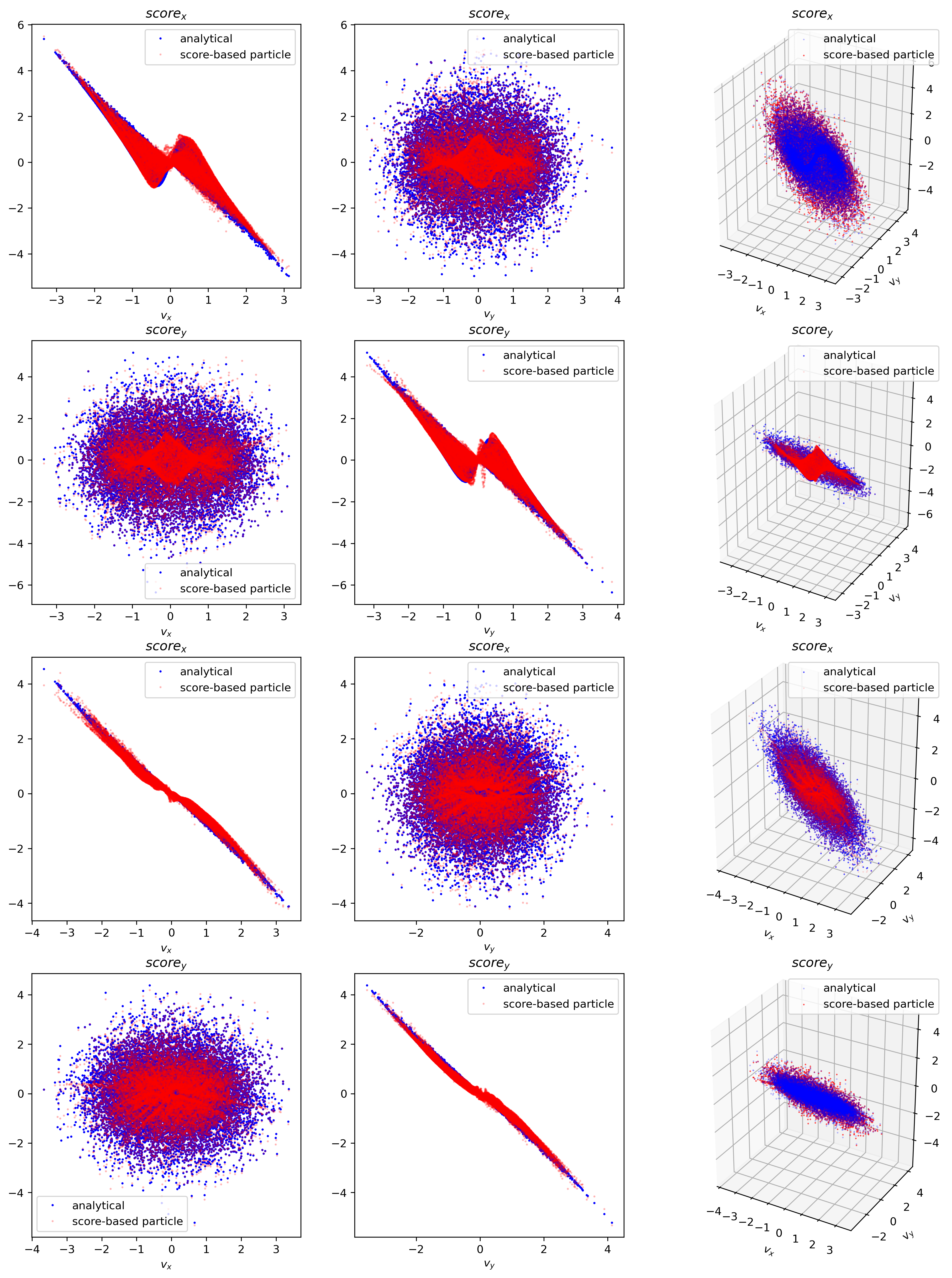
Figure 1: Score visualization. The first two rows are at $t=1$, the last two rows are at $t=5$.

To measure the accuracy of the learned score over time, we measure the goodness of fit using the relative Fisher divergence defined by

$$\frac{\int_{\mathbb{R}^{d}}|{\boldsymbol{s}}_{t}({\boldsymbol{v}})-\nabla\log\tilde{f}_{t}({\boldsymbol{v}})|^{2}f_{t}({\boldsymbol{v}})\mathrm{d}{\boldsymbol{v}}}{\int_{\mathbb{R}^{d}}|\nabla\log\tilde{f}_{t}({\boldsymbol{v}})|^{2}f_{t}({\boldsymbol{v}})\mathrm{d}{\boldsymbol{v}}}\approx\frac{\sum_{i=1}^{N}|{\boldsymbol{s}}_{n}({\boldsymbol{v}}_{i}^{n})-\nabla\log\tilde{f}_{t_{n}}({\boldsymbol{v}}_{i}^{n})|^{2}}{\sum_{i=1}^{N}|\nabla\log\tilde{f}_{t_{n}}({\boldsymbol{v}}_{i}^{n})|^{2}}.$$ (23)

This metric is plotted in Fig. 2, which demonstrates that the learned score closely matches the analytical score throughout the simulation duration.

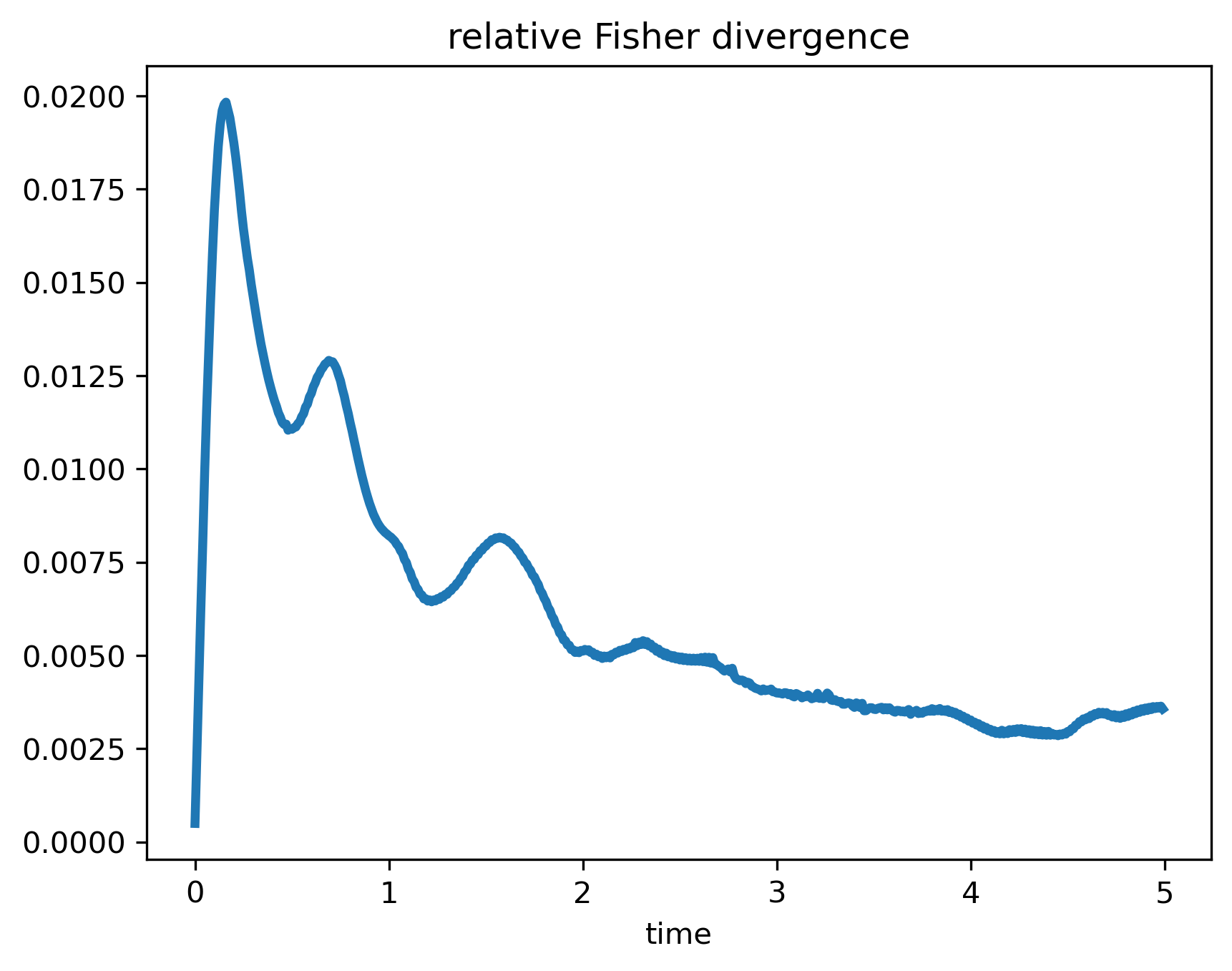
Figure 2: The evolution of the relative Fisher divergence (23).

The locations of particles at different time are displayed in Fig. 3.

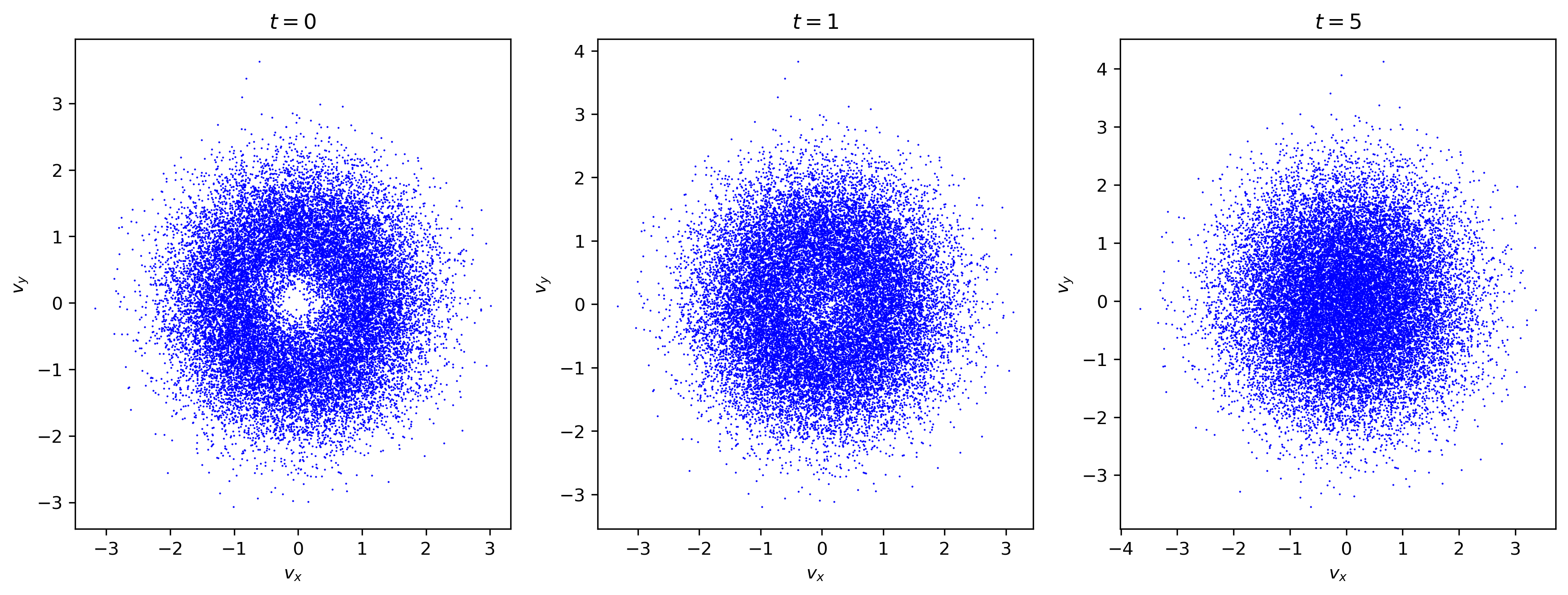
Figure 3: The location of particles at different time.

To further check the conservation and entropy decay properties of the method, we plot the time evolution of the total energy and the entropy decay rate in Fig. 4. The energy is conserved up to a small error while the entropy decay rate matches the analytical one (computed using (3) with quadrature rule).

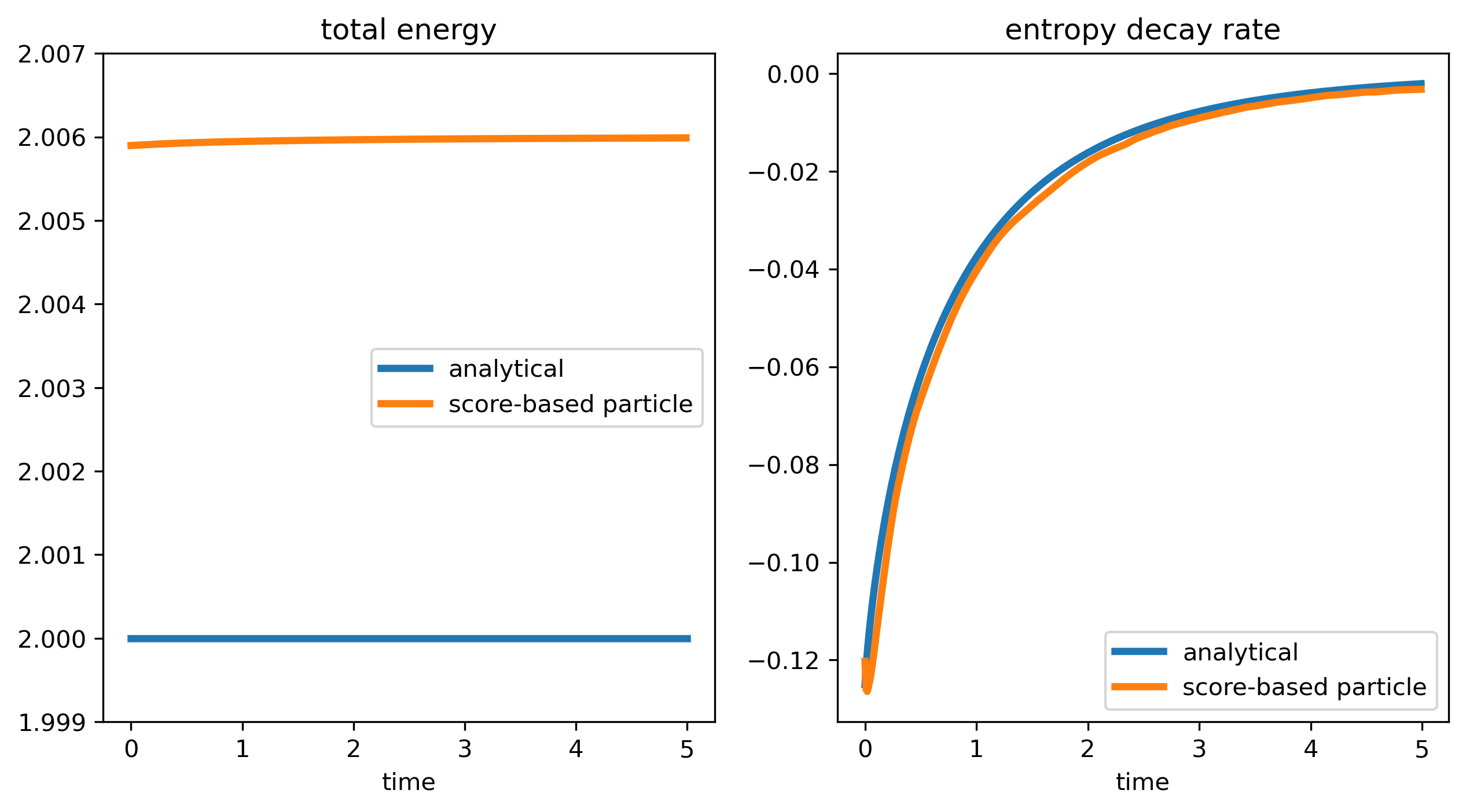
Figure 4: The evolution of the total energy (left) and the entropy decay rate (right).

Further, as is done in [8], we construct a KDE solution on the computational domain $[-L,L]^{2}$ with $L=4$, and uniformly divide the domain into $n=100^{2}$ meshes $\{Q_{i}\}_{i=1}^{n}$. The bandwidth of the Gaussian kernel is chosen to be $\varepsilon=0.15$. In Fig. 5, we track the discrete relative $L^{2}$-error between the analytical solution and the KDE solution defined by

$$\frac{\sqrt{\sum_{i=1}^{n}|\tilde{f}_{t}({\boldsymbol{v}}_{i}^{c})-\tilde{f}_{t}({\boldsymbol{v}}_{i}^{c})|^{2}}}{\sqrt{\sum_{i=1}^{n}|\tilde{f}_{t}({\boldsymbol{v}}_{i}^{c})|^{2}}},$$ (24)

where ${\boldsymbol{v}}_{i}^{c}$ is the center of $Q_{i}$.

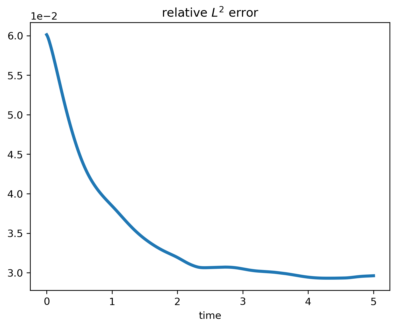
Figure 5: Time evolution of the relative $L^{2}$-error.

Finally in Fig. 6, we depict the slices of the solutions at different times. The plots demonstrate a close alignment between the KDE solutions and the analytical solutions.

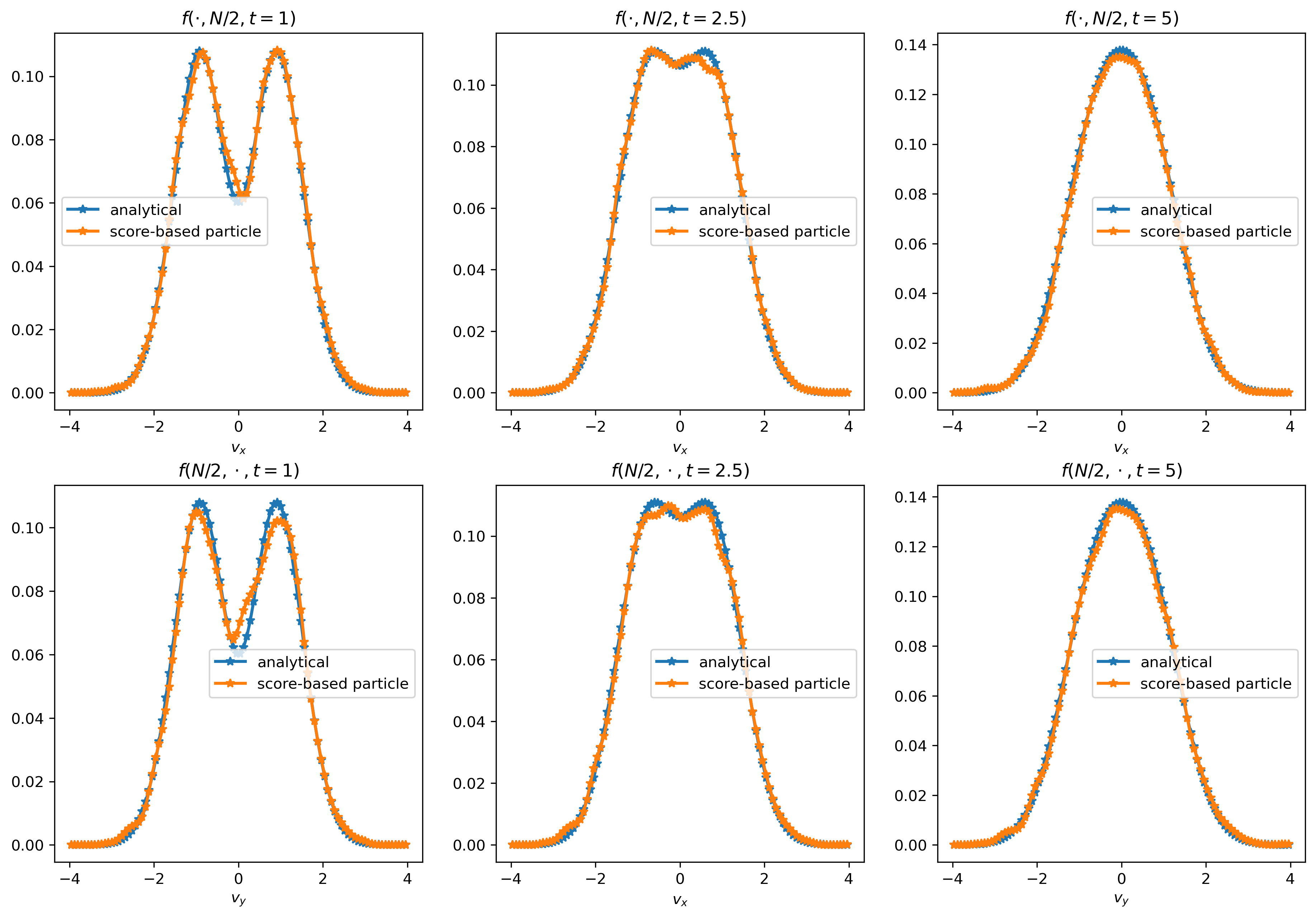
Figure 6: Slices of the numerical and analytical solutions at $t=1$, $2.5$, $5$.

5.2 Example 2: 3D BKW solution for Maxwell molecules

Consider the collision kernel

$$A(z)=\frac{1}{24}(|z|^{2}I_{d}-z\otimes z),$$

and an exact solution given by

$$\tilde{f}_{t}({\boldsymbol{v}})=\frac{1}{(2\pi K)^{3/2}}\exp\left(-\frac{|v|^{2}}{2K}\right)\left(\frac{5K-3}{2K}+\frac{1-K}{2K^{2}}|v|^{2}\right),\quad K=1-\exp(-t/6).$$

Setting.  In this test, we set $t_{0}=5.5$ and compute the solution until $t_{end}=6$. The time step is $\Delta t=0.01$. The total number of particles is $N=30^{3}$, initially i.i.d. sampled from $\tilde{f}_{5.5}$ by rejection sampling. The architecture of score ${\boldsymbol{s}}_{t}$ is a fully-connected neural network with $2$ hidden layers, $32$ neurons per hidden layer, and swish activation function. The initialization is identical to the first example. We train the neural networks using Adamax optimizer with a learning rate of $\eta=10^{-4}$, loss tolerance $\delta=5\times 10^{-4}$ for the initial score-matching, and the max iteration numbers $I_{\max}=15$ for the following implicit score-matching.

Comparison.  The time evolution of the relative Fisher divergence, the conserved total energy, and the entropy decay rate are shown in Fig. 7.

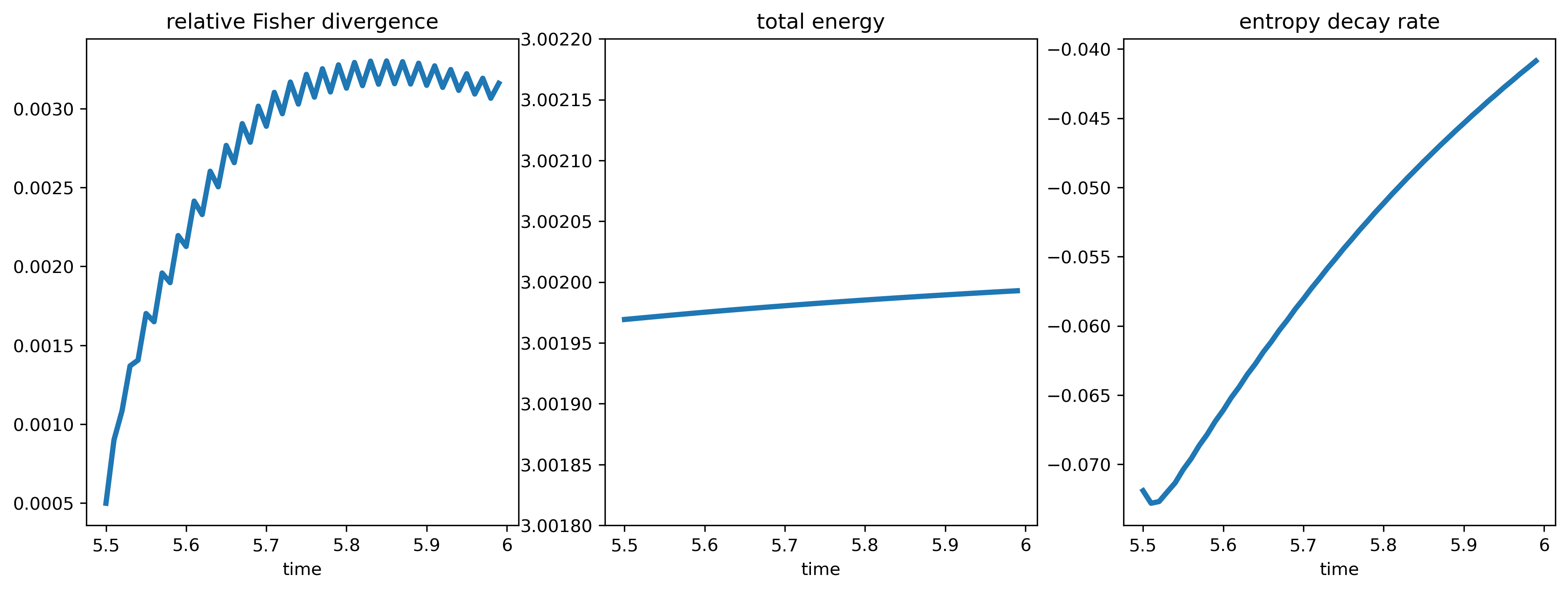
Figure 7: Time evolution of the relative Fisher divergence (left), the total energy (middle), and the entropy decay rate (right).

We construct a KDE solution on the computational domain $[-L,L]^{3}$ with $L=4$, and uniformly divide the domain into $n=30^{3}$ meshes. The bandwidth of the Gaussian kernel is chosen to be $\varepsilon=0.18$. In Fig. 8, we plot a slice of the solution at $t=6$ and track the discrete relative $L^{2}$-error (defined in (24)) between the analytical solution and the KDE solution.

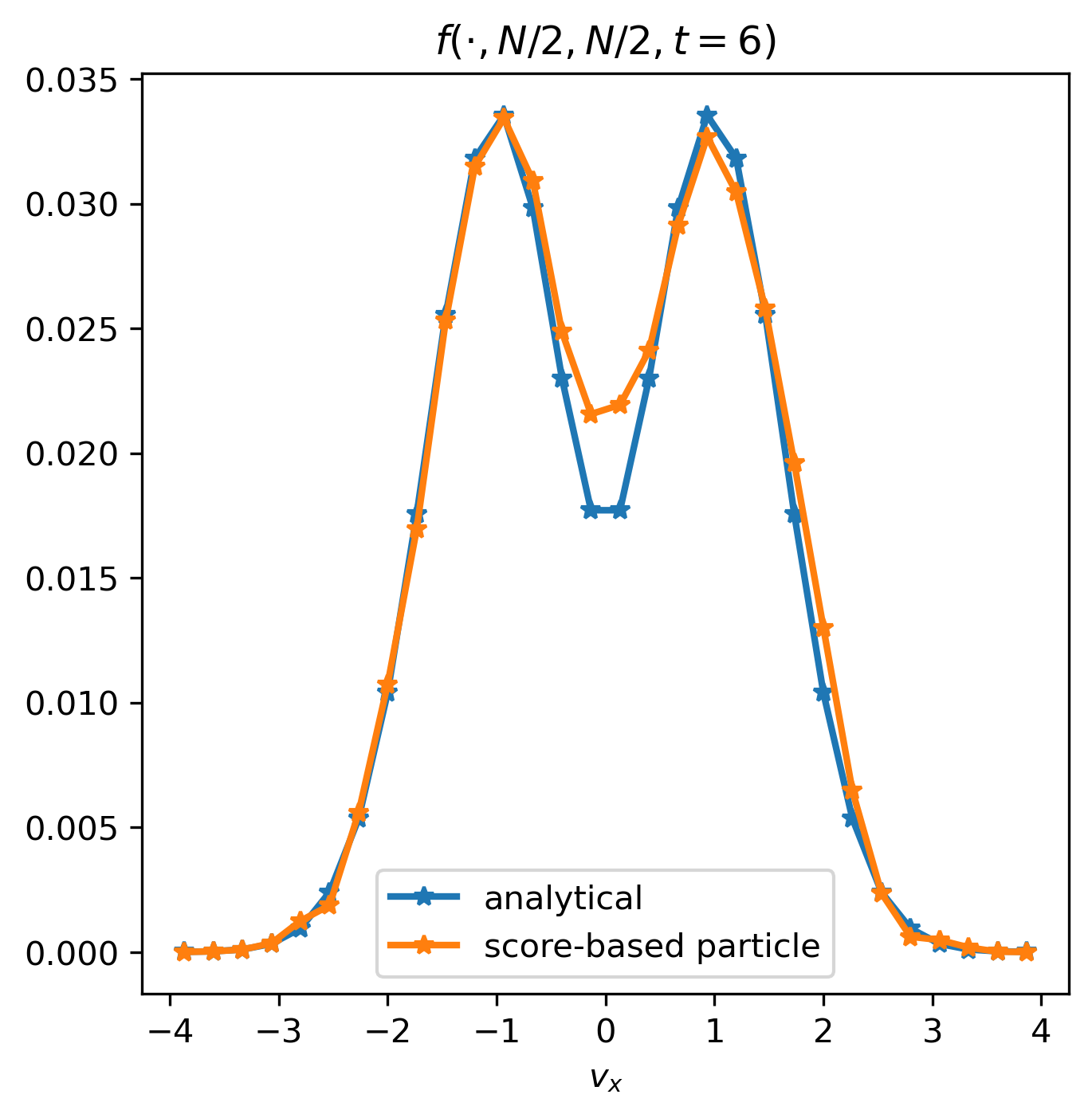
(a) Slice of the numerical and analytical solution at $t=6$.

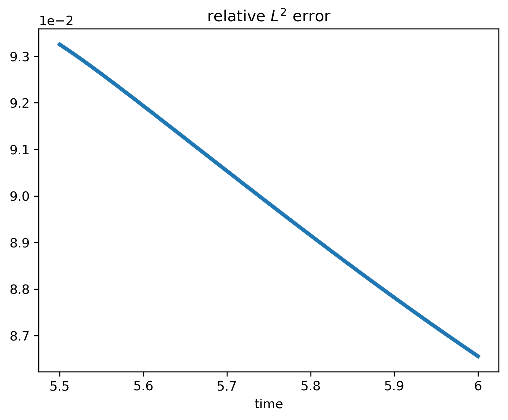
(b) Time evolution of the relative $L^{2}$-error.

Figure 8: Comparison of the numerical solution with the analytical solution.

5.3 Example 3: 2D anisotropic solution with Coulomb potential

Consider the Columb collision kernel

$$A(z)=\frac{1}{16}\frac{1}{|z|^{3}}(|z|^{2}I_{d}-z\otimes z),$$

and the initial condition given by a bi-Maxwellian

$$f_{0}({\boldsymbol{v}})=\frac{1}{4\pi}\left\{\exp\left(-\frac{|{\boldsymbol{v}}-u_{1}|^{2}}{2}\right)+\exp\left(-\frac{|{\boldsymbol{v}}-u_{2}|^{2}}{2}\right)\right\},\quad u_{1}=(-2,1),\quad u_{2}=(0,-1).$$

Setting.  In this experiment, we start from $t_{0}=0$ and compute the solution until $t_{end}=40$, with time step $\Delta t=0.1$. We choose the number of particles as $N=100^{2}$, sampled from $f_{0}$. We use a fully-connected neural network with $2$ hidden layers, $32$ neurons per hidden layer, and swish activation function to approximate the score ${\boldsymbol{s}}_{t}$. The initialization is identical to the first example. We train the neural networks using Adamax optimizer with a learning rate of $\eta=10^{-4}$, loss tolerance $\delta=10^{-5}$ for the initial score-matching, and the max iteration numbers $I_{\max}=25$ for the following implicit score-matching.

Result.  We construct a KDE solution on the computational domain $[-L,L]^{2}$ with $L=10$, and uniformly divide the domain into $n=128^{2}$ meshes. The bandwidth of the Gaussian kernel is chosen to be $\varepsilon=0.3$. The result in Fig. 9 closely resembles the findings in deterministic particle method and even the spectral method presented in [8].

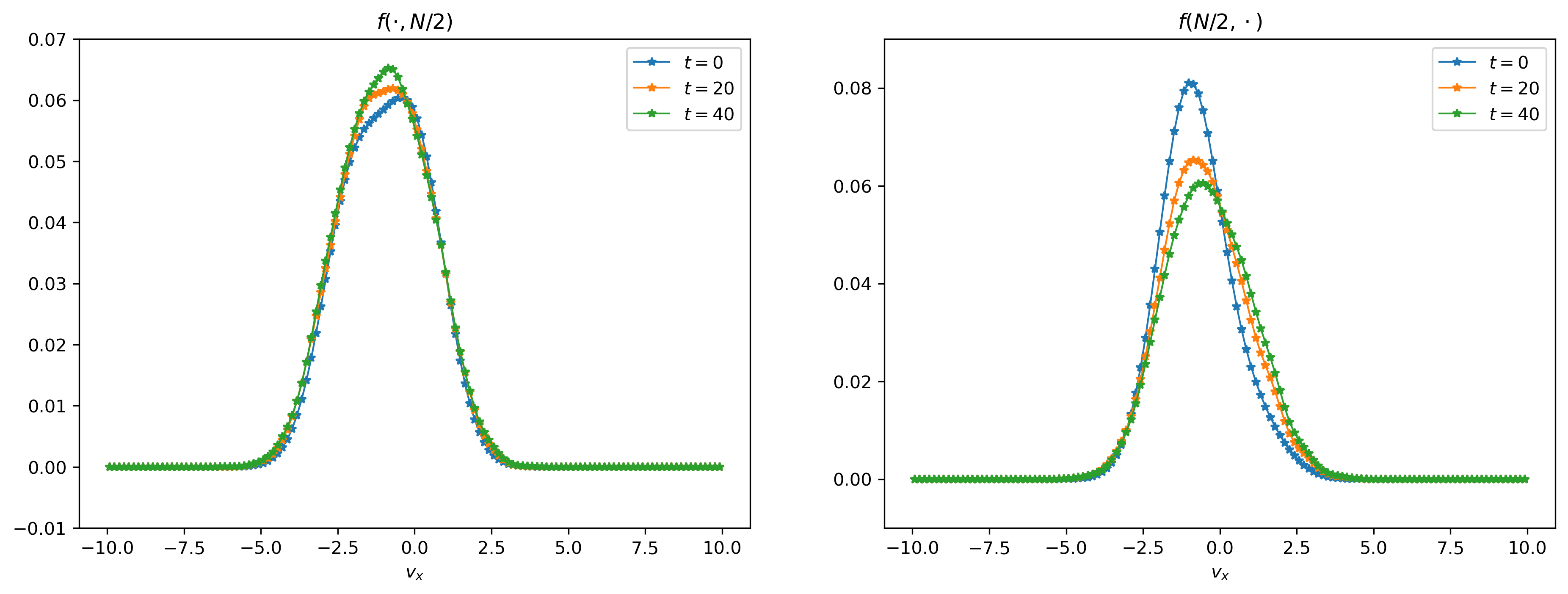
Figure 9: Slices of the numerical and analytical solutions at $t=0$, $20$, $40$.

5.4 Example 4: 3D Rosenbluth problem with Coulomb potential

Consider the collision kernel

$$A(z)=\frac{1}{4\pi}\frac{1}{|z|^{3}}(|z|^{2}I_{d}-z\otimes z),$$

and the initial condition

$$f_{0}({\boldsymbol{v}})=\frac{1}{S^{2}}\exp\left(-S\frac{(|{\boldsymbol{v}}|-\sigma)^{2}}{\sigma^{2}}\right),\quad\sigma=0.3,\quad S=10.$$

Setting.  In the example, we start from $t_{0}=0$ and compute the solution until $t_{end}=20$, with time step $\Delta t=0.2$. $N=30^{3}$ are initially sampled from $f_{0}$ by rejection sampling. The neural network approximating the score ${\boldsymbol{s}}_{t}$ is set to be a residue neural network [20] with $2$ hidden layers, $32$ neurons per hidden layer, and swish activation function. The initialization is identical to the first example. We train the neural networks using Adamax optimizer with a learning rate of $\eta=10^{-4}$, loss tolerance $\delta=5\times 10^{-4}$ for the initial score-matching, and the max iteration numbers $I_{\max}=25$ for the following implicit score-matching.

Result.  We construct a KDE solution on the computational domain $[-L,L]^{3}$ with $L=1$, and uniformly divide the domain into $n=64^{3}$ meshes. The bandwidth of the Gaussian kernel is chosen to be $\varepsilon=0.03$ for $t=10$ and $\varepsilon=0.05$ for $t=20$. In Fig. 10, we again observe a favorable agreement with the results presented in [8].

Efficiency.  To demonstrate the efficiency improvement in our approach, we compare the computation times for obtaining the score. In the score-based particle method, the total training time for the score is $42.835559$ seconds, utilizing PyTorch code on the Minnesota Supercomputer Institute Nvidia A40 GPU. In contrast, for the deterministic particle method [8], the computation time is approximately $5$ seconds per time step (with a total of $100$ time steps, resulting in approximately $500$ seconds for computing the score). These computations were performed using Matlab code on the Minnesota Supercomputer Institute Mesabi machine across $12$ nodes.

Nevertheless, we would like to point out that even though the score-based particle method speeds up score evaluation, the summation in $N$ on the right-hand side of (15) can be computationally expensive due to direct summations. To mitigate this, one could implement a treecode solver as demonstrated in [8], reducing the cost to $\mathcal{O}(N\log N)$, or adopt the random batch particle method proposed in [9], which reduces the cost to $\mathcal{O}(N)$. Since this paper primarily focuses on promoting the score-based concept, we leave further speed enhancements for future investigation.

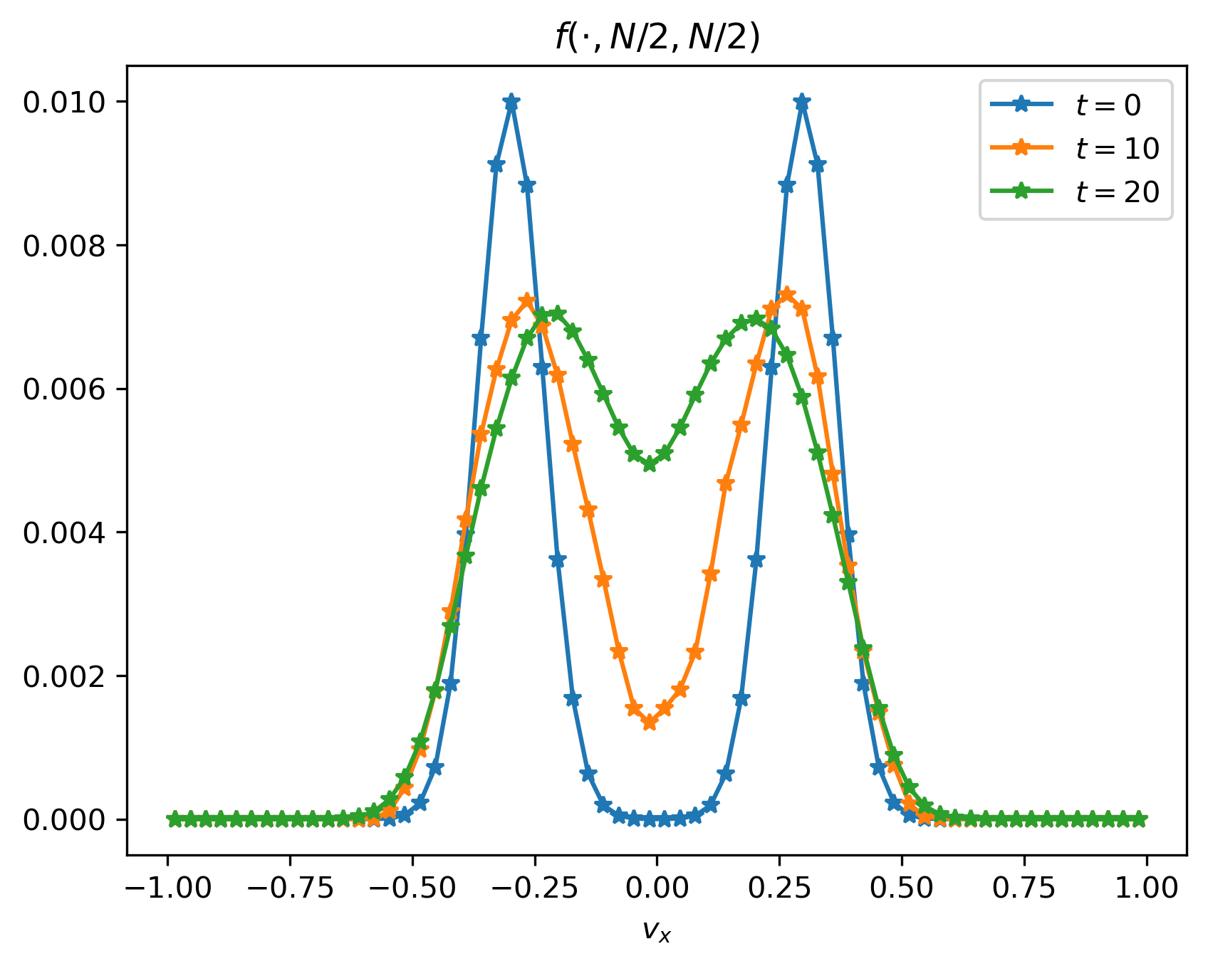
Figure 10: Slices of the solutions at $t=0$, $10$, $20$.

5.5 Density computation via Algorithm 2

This subsection is dedicated to investigating the density computation outlined in Section 4. We first examine the effectiveness of formula (line 5–6 in Algorithm 2) when the score function is provided exactly. To do so, we revisit the example in Section 5.1. If the exact score is available, then the only expected errors are the Monte Carlo error which scales as $\mathcal{O}(N^{-\frac{1}{2}})$ and time discretization error $\mathcal{O}(\Delta t)$. The same time step $\Delta t=0.01$ as in Section 5.1 is used for the subsequent tests.

We first track the relative $L^{1}$ and $L^{2}$ error of the solution with respect to particle numbers, and compute the convergence rate with respect to particle numbers at $t=1$, see Fig. 11. We observe the rate is slightly faster than the Monte Carlo convergence rate $\frac{1}{2}$.

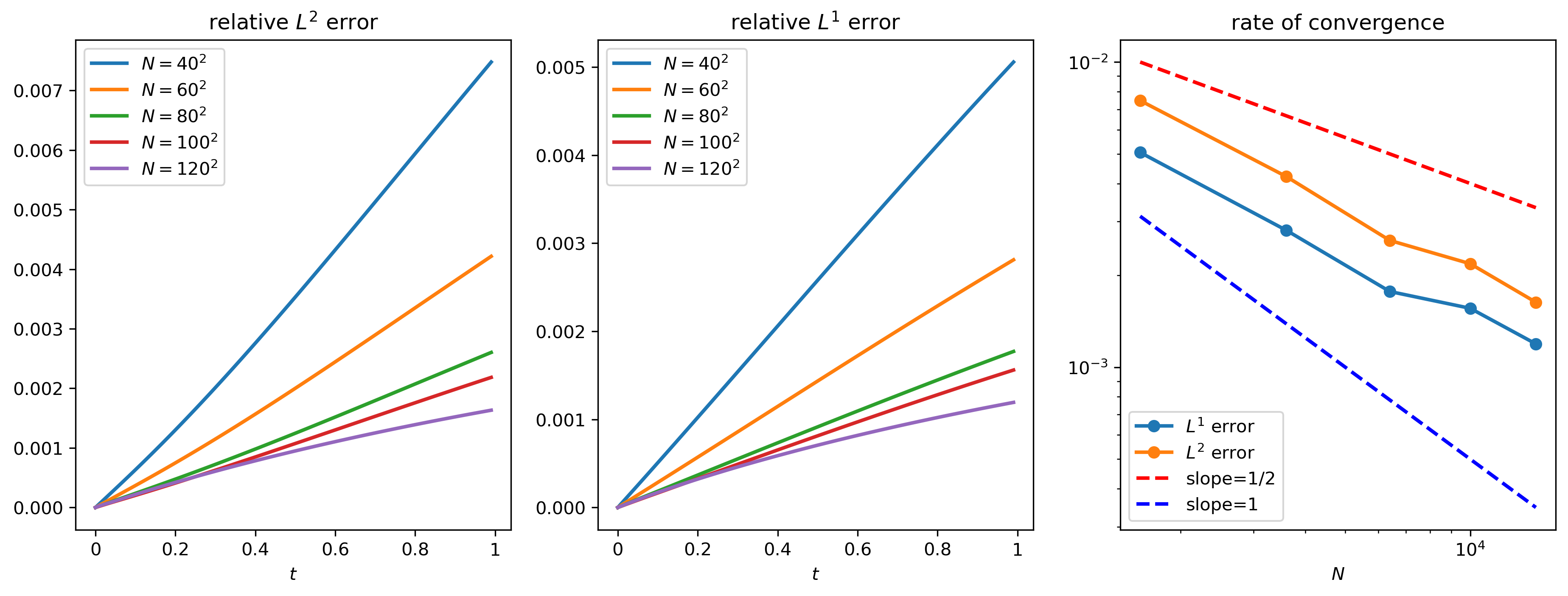
Figure 11: Time evolution of the relative $L^{1}$ and $L^{2}$ error with respect to particle numbers (left, middle); the rate of convergence with respect to particle numbers at $t=1$ (right).

To examine the long-term behavior of Algorithm 2, we compute the relative $L^{1}$ and $L^{2}$ errors (defined in (24) for $L^{2}$ and by removing the square in the formula for $L^{1}$) until $t=5$ using the same number of particles as in Section 5.1, as depicted in Fig. 12. It demonstrates that the error remains stable over time. We anticipate that better accuracy could be achieved by replacing the forward Euler time discretization with a higher-order method.

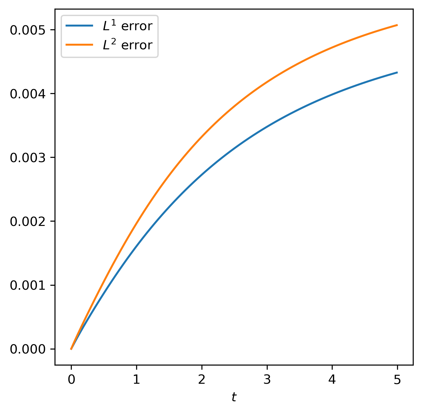
Figure 12: Long-term behavior of Algorithm 2.

Finally, we compare the numerical solution obtained by Algorithm 2 using the analytical score or score-matching with the analytical solution in Fig. 13. The experimental setup is identical to that in Section 5.1. Fig. 13a demonstrates that the numerical solution at $t=1$ obtained through Algorithm 2 using the analytical score closely overlaps with the analytical solution. In Fig. 13b, despite oscillations appearing near the top, the numerical solution still matches the analytical solution well. We attribute this to the fact that density computation uses the gradient of the score, while evolving particles only require the score itself, leading to higher accuracy demands on the score function for density computation. We defer the intriguing questions of how to learn the score function and its gradient with higher accuracy to future work.

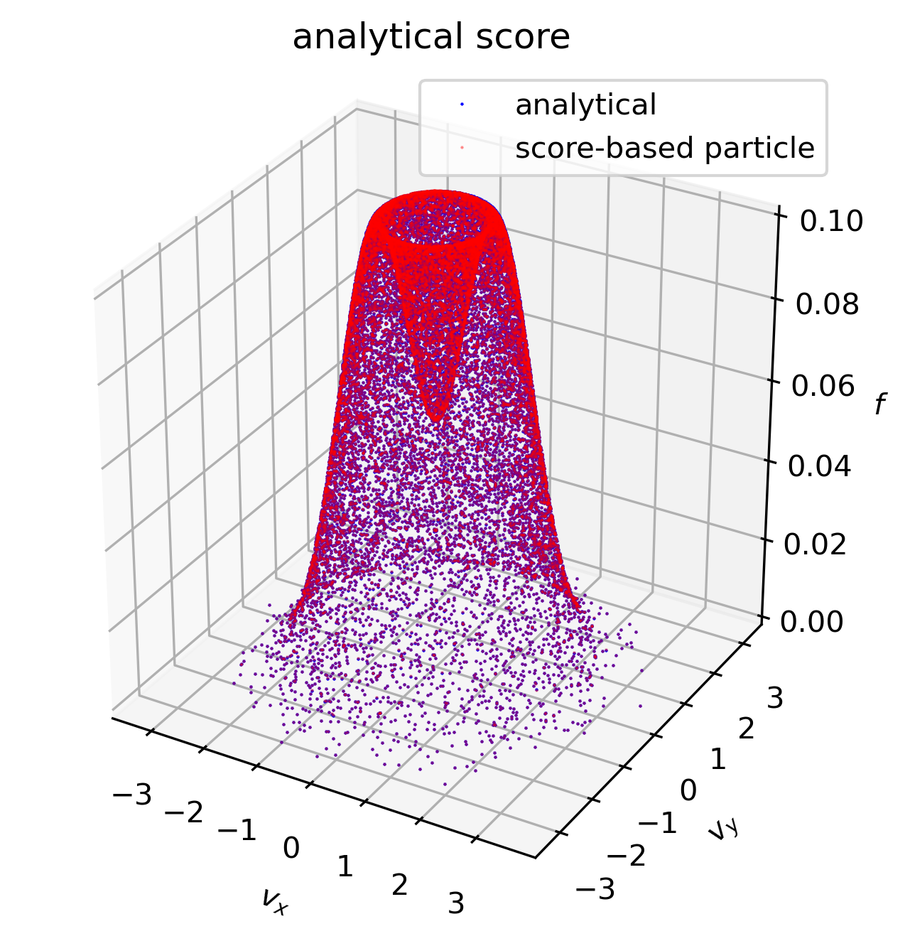
(a) Using analytical score.

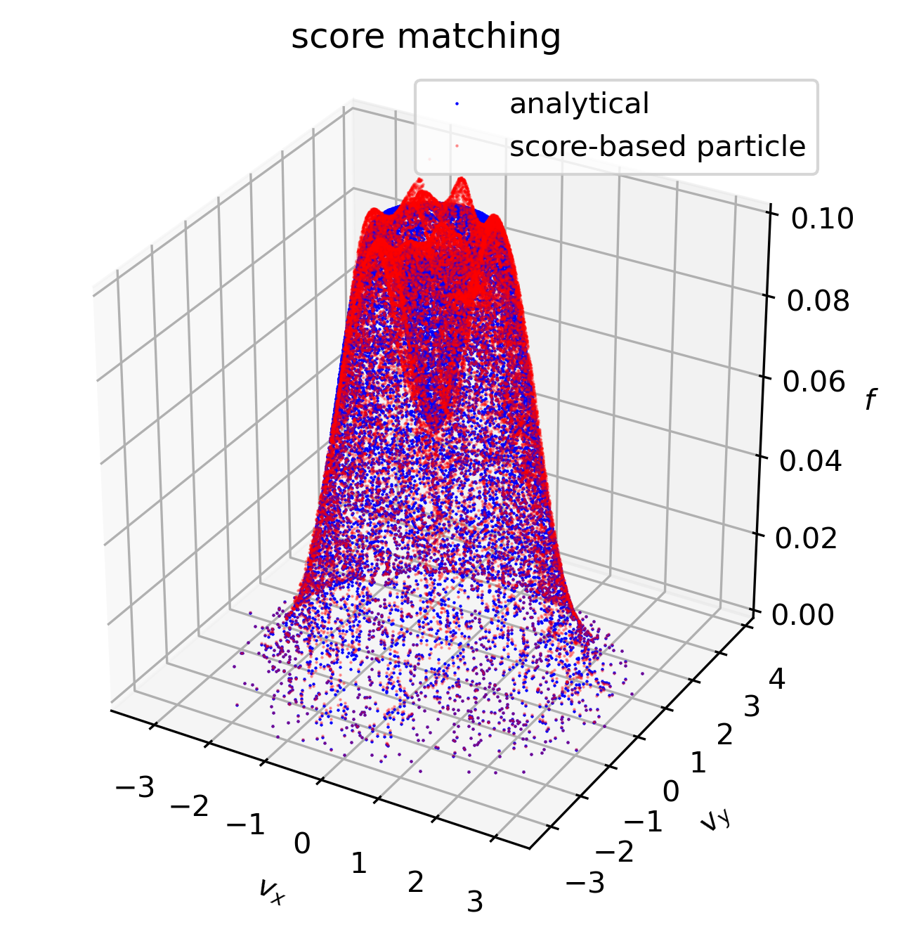
(b) Using neural network with score-matching.

Figure 13: Comparison of the analytical and numerical solutions obtained by Algorithm 2 at $t=1$.

Appendix A Proof of Corollary 4.2

Lemma A.1.

If $A(\boldsymbol{u})\in\mathbb{R}^{d\times d}$, $\boldsymbol{x}(\boldsymbol{u})\in\mathbb{R}^{d}$, and $\boldsymbol{u}\in\mathbb{R}^{d}$, then

$$\nabla_{\boldsymbol{u}}\cdot(A(\boldsymbol{u})\boldsymbol{x}(\boldsymbol{u}))=(\nabla_{\boldsymbol{u}}\cdot A(\boldsymbol{u})^{\top})\cdot\boldsymbol{x}(\boldsymbol{u})+A(\boldsymbol{u}):\nabla_{\boldsymbol{u}}\boldsymbol{x}(\boldsymbol{u})^{\top},$$

where $A:B:=\sum_{ij}A_{ij}B_{ij}$ and the divergence of matrix is applied row-wise.

Proof.

$$\begin{split}\nabla_{\boldsymbol{u}}\cdot(A(\boldsymbol{u})\boldsymbol{x}(\boldsymbol{u}))&=\frac{\mathrm{d}(a_{11}x_{1}+\cdots+a_{1d}x_{d})}{\mathrm{d}u_{1}}+\cdots+\frac{\mathrm{d}(a_{d1}x_{1}+\cdots+a_{dd}x_{d})}{\mathrm{d}u_{d}}\\ &=x_{1}\frac{\mathrm{d}a_{11}}{\mathrm{d}u_{1}}+\cdots+x_{d}\frac{\mathrm{d}a_{1d}}{\mathrm{d}u_{1}}+\cdots+x_{1}\frac{\mathrm{d}a_{d1}}{\mathrm{d}u_{d}}+\cdots+x_{d}\frac{\mathrm{d}a_{dd}}{\mathrm{d}u_{d}}+\\ &\quad+a_{11}\frac{\mathrm{d}x_{1}}{\mathrm{d}u_{1}}+\cdots+a_{1d}\frac{\mathrm{d}x_{d}}{\mathrm{d}u_{1}}+\cdots+a_{d1}\frac{\mathrm{d}x_{1}}{\mathrm{d}u_{d}}+\cdots+a_{dd}\frac{\mathrm{d}x_{d}}{\mathrm{d}u_{d}}\\ &=(\nabla_{\boldsymbol{u}}\cdot A(\boldsymbol{u})^{\top})\cdot\boldsymbol{x}(\boldsymbol{u})+A(\boldsymbol{u}):\nabla_{\boldsymbol{u}}\boldsymbol{x}(\boldsymbol{u})^{\top}.\end{split}$$

∎

Now we present the proof for Corollary 4.2.

Proof.

By Lemma A.1,

$$\nabla\cdot\left[\Pi(\boldsymbol{T}({\boldsymbol{V}},t)-\boldsymbol{T}({\boldsymbol{V}}_{*},t))\left(\tilde{\boldsymbol{s}}_{t}(\boldsymbol{T}({\boldsymbol{V}},t))-\tilde{\boldsymbol{s}}_{*t}(\boldsymbol{T}({\boldsymbol{V}}_{*},t))\right)\right]$$

$$= [\nabla\cdot\Pi(\boldsymbol{T}({\boldsymbol{V}},t)-\boldsymbol{T}({\boldsymbol{V}}_{*},t))^{\top}]\cdot(\tilde{\boldsymbol{s}}_{t}(\boldsymbol{T}({\boldsymbol{V}},t))-\tilde{\boldsymbol{s}}_{*t}(\boldsymbol{T}({\boldsymbol{V}}_{*},t)))+\Pi(\boldsymbol{T}({\boldsymbol{V}},t)-\boldsymbol{T}({\boldsymbol{V}}_{*},t)):\nabla\tilde{\boldsymbol{s}}_{t}(\boldsymbol{T}({\boldsymbol{V}},t))^{\top}$$

$$= [\nabla\cdot\Pi(\boldsymbol{T}({\boldsymbol{V}},t)-\boldsymbol{T}({\boldsymbol{V}}_{*},t))]\cdot(\tilde{\boldsymbol{s}}_{t}(\boldsymbol{T}({\boldsymbol{V}},t))-\tilde{\boldsymbol{s}}_{*t}(\boldsymbol{T}({\boldsymbol{V}}_{*},t)))+\Pi(\boldsymbol{T}({\boldsymbol{V}},t)-\boldsymbol{T}({\boldsymbol{V}}_{*},t)):\nabla\tilde{\boldsymbol{s}}_{t}(\boldsymbol{T}({\boldsymbol{V}},t))^{\top}.$$

Let $\boldsymbol{z}:=\boldsymbol{T}({\boldsymbol{V}},t)-\boldsymbol{T}({\boldsymbol{V}}_{*},t)$. Then

$$\Pi(\boldsymbol{z})=\frac{1}{z_{1}^{2}+z_{2}^{2}+z_{3}^{2}}\begin{pmatrix}z_{2}^{2}+z_{3}^{2}&-z_{1}z_{2}&-z_{1}z_{3}\\ -z_{1}z_{2}&z_{1}^{2}+z_{3}^{2}&-z_{2}z_{3}\\ -z_{1}z_{3}&-z_{2}z_{3}&z_{1}^{2}+z_{2}^{2}\end{pmatrix}\implies\nabla\cdot\Pi(\boldsymbol{z})=-\frac{\boldsymbol{z}}{|\boldsymbol{z}|^{2}}.$$

Therefore, the evolution for $\log|\det\nabla_{\boldsymbol{V}}\boldsymbol{T}({\boldsymbol{V}},t)|$ is

$$\frac{\mathrm{d}}{\mathrm{d}t}\log|\det\nabla_{\boldsymbol{V}}\boldsymbol{T}({\boldsymbol{V}},t)|=-\int_{\mathbb{R}^{d}}\bigg{\{}A(\boldsymbol{T}({\boldsymbol{V}},t)-\boldsymbol{T}({\boldsymbol{V}}_{*},t)):\nabla\tilde{\boldsymbol{s}}_{t}(\boldsymbol{T}({\boldsymbol{V}},t))^{\top}$$

$$-C_{\gamma}|\boldsymbol{T}({\boldsymbol{V}},t)-\boldsymbol{T}({\boldsymbol{V}}_{*},t)|^{\gamma}(\boldsymbol{T}({\boldsymbol{V}},t)-\boldsymbol{T}({\boldsymbol{V}}_{*},t))\cdot\left(\tilde{\boldsymbol{s}}_{t}(\boldsymbol{T}({\boldsymbol{V}},t))-\tilde{\boldsymbol{s}}_{*t}(\boldsymbol{T}({\boldsymbol{V}}_{*},t))\right)\bigg{\}}f_{0}({\boldsymbol{V}}_{*})\mathrm{d}{\boldsymbol{V}}_{*}.$$

∎

References

- [1] N. M. Boffi and E. Vanden-Eijnden, Probability flow solution of the fokker–planck equation, Machine Learning: Science and Technology, 4 (2023), p. 035012.
- [2] C. Buet and S. Cordier, Conservative and entropy decaying numerical scheme for the isotropic fokker–planck–landau equation, Journal of Computational Physics, 145 (1998), pp. 228–245.
- [3] J. A. Carrillo, K. Craig, and F. S. Patacchini, A blob method for diffusion, Calculus of Variations and Partial Differential Equations, 58 (2019), pp. 1–53.
- [4] J. A. Carrillo, M. G. Delgadino, L. Desvillettes, and J. S. H. Wu, The landau equation as a gradient flow, arXiv, (2022).
- [5] J. A. Carrillo, M. G. Delgadino, and J. Wu, Boltzmann to landau from the gradient flow perspective, Nonlinear Analysis, 219 (2022), p. 112824.
- [6] J. A. Carrillo, M. G. Delgadino, and J. S. H. Wu, Convergence of a particle method for a regularized spatially homogeneous landau equation, Mathematical Models and Methods in Applied Sciences, 33 (2023), pp. 971–1008.
- [7] J. A. Carrillo, S. Guo, and P.-E. Jabin, Mean-field derivation of landau-like equations, arXiv preprint arXiv:2403.12651, (2024).
- [8] J. A. Carrillo, J. Hu, L. Wang, and J. Wu, A particle method for the homogeneous landau equation, Journal of Computational Physics: X, 7 (2020), p. 100066.
- [9] J. A. Carrillo, S. Jin, and Y. Tang, Random batch particle methods for the homogeneous landau equation, Communications in Computational Physics, 31 (2022), pp. 997–1019.
- [10] R. T. Q. Chen, Y. Rubanova, J. Bettencourt, and D. K. Duvenaud, Neural ordinary differential equations, Advances in Neural Information Processing Systems, 31 (2018).
- [11] P. Degond and B. Lucquin-Desreux, The fokker-planck asymptotics of the boltzmann collision operator in the coulomb case, Mathematical Models and Methods in Applied Sciences, 2 (1992), pp. 167–182.
- [12] , An entropy scheme for the fokker-planck collision operator of plasma kinetic theory, Numerische Mathematik, 68 (1994), pp. 239–262.
- [13] L. Desvillettes and C. Villani, On the spatially homogeneous landau equation for hard potentials part i : existence, uniqueness and smoothness, Communications in Partial Differential Equations, 25 (2000), pp. 179–259.
- [14] , On the spatially homogeneous landau equation for hard potentials part ii : h-theorem and applications, Communications in Partial Differential Equations, 25 (2000), pp. 261–298.
- [15] G. Dimarco, R. Caflisch, and L. Pareschi, Direct simulation monte carlo schemes for coulomb interactions in plasmas, arXiv preprint arXiv:1010.0108, (2010).
- [16] W. E and B. Yu, The deep ritz method: A deep learning-based numerical algorithm for solving variational problems, Communications in Mathematics and Statistics, 6 (2018), pp. 1–12.
- [17] W. Grathwohl, R. T. Q. Chen, J. Bettencourt, and D. Duvenaud, Scalable reversible generative models with free-form continuous dynamics, International Conference on Learning Representations, (2019).
- [18] M. P. Gualdani and N. Zamponi, Spectral gap and exponential convergence to equilibrium for a multi-species landau system, Bulletin des Sciences Mathématiques, 141 (2017), pp. 509–538.
- [19] Y. Guo, The landau equation in a periodic box, Communications in Mathematical Physics, 231 (2002), pp. 391–434.
- [20] K. He, X. Zhang, S. Ren, and J. Sun, Deep residual learning for image recognition, 2016 IEEE Conference on Computer Vision and Pattern Recognition (CVPR), (2016), pp. 770–778.
- [21] A. Hyvärinen, Estimation of non-normalized statistical models by score matching, Journal of Machine Learning Research, 6 (2005), pp. 695–709.
- [22] S. Ioffe and C. Szegedy, Batch normalization: Accelerating deep network training by reducing internal covariate shift, Proceedings of the 32nd International Conference on Machine Learning, 37 (2015), pp. 448–456.
- [23] S. Jin, Z. Ma, and K. Wu, Asymptotic-preserving neural networks for multiscale time-dependent linear transport equations, Journal of Scientific Computing, 94 (2023), p. 57.
- [24] S. Jin, Z. Ma, and K. Wu, Asymptotic-preserving neural networks for multiscale kinetic equations, Communications in Computational Physics, 35 (2024), pp. 693–723.
- [25] S. Jin, Z. Ma, and T.-a. Zhang, Asymptotic-preserving neural networks for multiscale vlasov–poisson–fokker–planck system in the high-field regime, Journal of Scientific Computing, 99 (2024), p. 61.
- [26] D. P. Kingma and J. Ba, Adam: A method for stochastic optimization, arXiv, (2017).
- [27] L. D. Landau, The kinetic equation in the case of coulomb interaction., tech. rep., General Dynamics/Astronautics San Diego Calif, 1958.
- [28] W. Lee, L. Wang, and W. Li, Deep jko: time-implicit particle methods for general nonlinear gradient flows, arXiv preprint arXiv:2311.06700, (2023).
- [29] L. Li, S. Hurault, and J. M. Solomon, Self-consistent velocity matching of probability flows, Advances in Neural Information Processing Systems, 36 (2023), pp. 57038–57057.
- [30] J. Lu, Y. Wu, and Y. Xiang, Score-based transport modeling for mean-field fokker-planck equations, Journal of Computational Physics, 503 (2024), p. 112859.
- [31] Y. Lu, L. Wang, and W. Xu, Solving multiscale steady radiative transfer equation using neural networks with uniform stability, Research in the Mathematical Sciences, 9 (2022), p. 45.
- [32] L. Pareschi, G. Russo, and G. Toscani, Fast spectral methods for the fokker–planck–landau collision operator, Journal of Computational Physics, 165 (2000), pp. 216–236.
- [33] M. Raissi, P. Perdikaris, and G. Karniadakis, Physics-informed neural networks: A deep learning framework for solving forward and inverse problems involving nonlinear partial differential equations, Journal of Computational Physics, 378 (2019), pp. 686–707.
- [34] P. Ramachandran, B. Zoph, and Q. V. Le, Searching for activation functions, arXiv, (2017).
- [35] Z. Shen and Z. Wang, Entropy-dissipation informed neural network for mckean-vlasov type PDEs, Thirty-seventh Conference on Neural Information Processing Systems, (2023).
- [36] Z. Shen, Z. Wang, S. Kale, A. Ribeiro, A. Karbasi, and H. Hassani, Self-consistency of the fokker planck equation, Proceedings of Thirty Fifth Conference on Learning Theory, 178 (2022), pp. 817–841.
- [37] J. Sirignano and K. Spiliopoulos, Dgm: A deep learning algorithm for solving partial differential equations, Journal of Computational Physics, 375 (2018), pp. 1339–1364.
- [38] Y. Song and S. Ermon, Generative modeling by estimating gradients of the data distribution, Advances in Neural Information Processing Systems, 32 (2019).
- [39] , Improved techniques for training score-based generative models, Advances in Neural Information Processing Systems, 33 (2020), pp. 12438–12448.
- [40] Y. Song, J. Sohl-Dickstein, D. P. Kingma, A. Kumar, S. Ermon, and B. Poole, Score-based generative modeling through stochastic differential equations, International Conference on Learning Representations, (2021).
- [41] C. Villani, On a new class of weak solutions to the spatially homogeneous boltzmann and landau equations, Archive for Rational Mechanics and Analysis, 143 (1998), pp. 273–307.
- [42] P. Vincent, A connection between score matching and denoising autoencoders, Neural Computation, 23 (2011), pp. 1661–1674.
- [43] Y. Zang, G. Bao, X. Ye, and H. Zhou, Weak adversarial networks for high-dimensional partial differential equations, Journal of Computational Physics, 411 (2020), p. 109409.