Asymmetric Symmetry Breaking:
Unequal Probabilities of Vacuum Selection
Abstract
Spontaneous symmetry breaking is a fundamental notion in modern physics, ranging from high energy to condensed matter. However, the usual spontaneous symmetry breaking only considers the equal probability to select the vacua. In this work, we conceive a model to realize the unequal probability of the symmetry breaking, leading to an unbalanced number of ground states. Specifically, we study the probabilities of a scalar field to roll down from the top of a potential, where the top is only continuous. As the whole system is subject to random perturbations, we find that the probability for the field to roll down to the left or right side depends the square root of the second derivative of the potential at the top. We solve this problem theoretically by using the Fokker-Planck equations in stochastic process and verify our findings numerically. This study may potentially be a new mechanism to explain the origins of asymmetries in the Universe.
Spontaneous symmetry breaking (SSB) is an important concept in contemporary physics. It is vital for the Higgs mechanism in particle physics [1, 2], the cosmological phase transitions in cosmology [3], the superconducting phenomena in condensed matter physics [4] and the formation of topological defects in nonequilibrium dynamics [5, 6, 7], etc. A typical picture of SSB is a field to roll down a potential with Mexican-hat profile. The field was sitting at the top of the potential initially with higher symmetries. Since the top is unstable, the field will then roll down the potential randomly and settle down in one of the lowest energy states, aka ground states. Compared to the symmetries at the top, the chosen state has lower symmetries, thus, symmetry was broken. We call this process of SSB as “vacuum selection”.
Commonly, the probabilities for the field to roll down the potential are identical, that is to say, the probabilities of the vacuum selection are equal. For instance, if the potential is only one-dimensional, then the filed to roll down from the top to the left or right side are exactly one-half. A natural question is: how can it have unequal probabilities for the vacuum selection? This can be equivalently expressed as how can the field have the unequal probabilities to roll down the potential. If it can be realized, it may have important meanings to the physics of symmetry breaking, since ground states are overarching in quantum field theory [8, 9].
In this work, we utilize an artificial Higgs-type potential to realize the unequal probabilities of the vacuum selection. For simplicity, we will only consider one-dimensional potential. In particular, the top of the potential is only continuous, but discontinuous at higher order, like the sketchy picture shows in Fig.1. We call this potential as “ continuous”, in which the upper circle indicates that only the top is continuous while other parts are continuous.
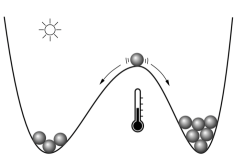
We assume that the whole system is subject to random external forces, for example coupled to a thermal reservoir. Under the random perturbations, the field at the top will have the probability to roll down to the left or right side. And eventually settle down to the lower energy states at the minimum of the potential. In this work, we use the Fokker-Planck equation in stochastic process [10] to solve this problem theoretically, and find that the probability for the field to roll down to the left (right) depends on the square root of the second derivative of the potential at the left (right) side of the top. Then we adopt the time-dependent Ginzburg-Landau model [11] for real scalar fields to simulate this process by virtue of the Higgs-type potential. From this model, we see that the numerical results are consistent with the theoretical predictions very well.
I Theory
We consider the time-dependent Ginzburg-Landau equation with an external random force ,
| (1) |
where is a real scalar field, is a coefficient related to the dissipations and is the potential. The random force satisfies the Gaussian white noise relation where is the fluctuation strength. If the random perturbation comes from the thermal fluctuations of a heat bath, will be linearly proportional to the temperature due to the fluctuation-dissipation theorem [12], i.e., where we have set the Boltzmann constant .
From stochastic process, the probability to find the field in the range at some instant satisfies the Fokker-Planck equation [10],
| (2) |
Assume that at initial time the field is sitting at the top of the potential like in Fig.1, because of the random fluctuations the field is unstable and will eventually roll down the potential to the left or right side. Without loss of generality, we can always translate the top of the potential to be seated at . Intuitively, the probability for the field to roll down to the left (right) of potential will only depends on the profile of the top and its vicinity, and has nothing to do with the far-away regions from the top. Therefore, we can expand the potential near the top , i.e., , where the symbol ′ indicates the derivative of with respect to and the subscripts imply that the values are taken at . Since the top is a maximum, we get . Hence, . Therefore, the corresponding Fokker-Planck equation Eq.(2) reduces to
| (3) |
In the Eq.(3) we have ignored the higher terms of the expansion in since they make minor contributions compared to the linear term of near .
Imagine that we make plenty of experiments to roll down the fields from the top, after enough times of the experiments we can find that the probability of rolling down to the left (right) of the potential will reach a stationary value, i.e, . From the reduced Fokker-Plank equation Eq.(3), the stationary solution is
| (4) |
It should be noted that the above solution is only valid nearby the top of the potential.
At the initial time sits at the top of the potential where . Then we evolve the system to see whether will roll down to the left or right. Random fluctuations of in this case plays a role of disturbing from to , where is a relatively small value. If is negative (positive), the field will roll to the left (right) and then roll down the potential persistently until the left (right) minimum. 111This behavior can be intuitively seen in the inset plot of the following Fig.2 b. Since is small, we can ignore the exponential term in the Eq.(4). Therefore, we can speculate that the probability to roll down to the left (right) directly depends the factor . Now consider that the potential is only continuous, then the second derivative of the potential near are different on each side of the top. We can define at , and then get
| (5) |
where indicates the probability of rolling down to the left (right) side. We have omitted the symbols of absolute value since the ratio are positive although they are individually negative. Since , it is readily to obtain from the Eq.(5) that
| (6) |
Or, equivalently, .
II Numerical Evidences
In the following we will use an effective potential to verify our conclusions, i.e., Eq.(5) and (6) above. Specifically, the potential is the Higgs-type potential as,
| (7) | |||||
where is the Heaviside step function with
| (11) |
One may find that the Higgs-type potential is not symmetric under , therefore the original system is not symmetric under transformation. Strictly speaking, this is not even a symmetry breaking. However, we need to stress that our starting point is from the time-dependent Ginzburg-Landau equation rather than from the Lagrangian or Hamiltonian formalism. We adopt the effective asymmetric potential to learn the probabilities of the field to roll down to the left or right. Nevertheless, in order to compare our study to the ordinary “symmetry breaking” with equal probabilities, we deliberately call our case as “asymmetric symmetry breaking”. The meaning of it can be understood from this aspect.
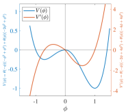
In numerics, we fix and vary in the range of . Please find the profile of the potential (blue) and its derivative (red) in the Fig.2 a, in which we set . Obviously, the profile of the potential satisfies the requirement of continuous. This potential has two minima and which are exactly the positive and negative vacuum values. In the numerics, we use the 4-th Runge-Kutta methods to evolve the system. And we have set the time step as , the coefficient and the temperature . For the counting statistics, we independently simulate the dynamics for 30000 times.
In the panel b of Fig.2 we show the time evolution of the scalar fields with the potential in panel a. In this plot we show three cases for the scalar field to select the positive vacuum and three cases for selecting the negative vacuum. Because of the random temperature perturbations, each three lines are not completely overlap. But at the final time they will overlap and reach the equilibrium values of the positive (negative) vacuum, respectively. The positive (negative) equilibrium value is () which are exactly the value of () corresponding to the two minima of the potential. In the inset plot of panel b we show the early evolutions of two cases of the fields. We can see that in the very early time the fields will fluctuate around due to the external temperature perturbations. But this fluctuation near the top of the potential will not last long enough time because they are unstable at the top. At certain time they will go away from the top at , and then persistently roll down the hill until meeting the minimum of the potential. The arrows in the inset plot imply the persistence of rolling down the hill. Finally, they will settle down at the minima of the potential, which is reflected by staying at the plateaus in panel b.
Panel c of Fig.2 shows the relation between and . From the potential Eq.(7) we see that at the top of the potential. From panel c we see that the numerical results (circles) match the theoretical prediction (red line) very well. Fig.2 c demonstrates the theoretical prediction in Eq.(6).
Panel d of Fig.2 exhibits the relation between and . Therefore, we see that the numerical data (circles) also match the theoretical prediction (red line) very well. The inset plot in panel d shows the double logarithmic plots of the relation, and the slope exactly means the square root relation in . Fig.2 d verifies the theoretical prediction in Eq.(5).
II.1 Counting statistics of the binomial distribution
If we regard the rolling down to the right side as a success with probability , then rolling down to the left is a failure with probability . Therefore, each time of the rolling down is a Bernoulli trial. Then after times of trials, the probability of rolling down to the right side as times should satisfy the binomial distributions [13]
| (12) |
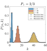
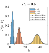
In Fig.3 we show the counting statistics of the rolling down to the right side with the Higgs-type potential. In the left column, i.e., Fig.3 a and c, we set and . Therefore, according to our theoretical prediction in Eq.(6), the probability of rolling down to the right side is . While in the right column, i.e., Fig.3 b and d, we set and , thus . Panel a and b of Fig.3 show the histogram of the probability , which means the probability for times of rolling down to the right side in trials. We can see that for different probabilities and different trial numbers , the histogram of are consistent with the theoretical binomial distributions in Eq.(12) very well. We did not show the error bars of the histogram since the errors are very tiny.
Fig.3 c and d exhibit the extremal cases that there are no events for rolling down to the right side in trials, i.e., , for different . Theoretically, from the binomial distribution Eq.(12), this probability for vanishing should be . From Fig.3 c and d, we see that the numerical statistics (circles) match the theoretical predictions (red lines) very well. The inset plots show the relations between and . From the binomial distribution, the theoretical relation should be , which are reflected by the linear relations in the inset plots. Moreover, the slopes are consistent with the theoretical predictions. Specifically, the slopes are in Fig.3 c and in Fig.3 d, respectively.
Therefore, we see that the binomial distributions with the given probability are consistent with the numerical statistics. This in turn implies that our theoretical prediction in Eq.(5) and Eq.(6) are correct.
We must stress that our main findings in Eq.(5) and Eq.(6) are robust against by varying other parameters. In numerics, we already checked that they are robust against: (I) varying the reservoir temperature ; (II) varying the coefficient ; (III) adding terms in the potential Eq.(7); (IV) changing the coefficients in front of ; (V) adding higher order terms in the potential, such as and etc. In the Supplemental Materials we adopt another cosine-type potential to numerically verifies our theoretical predictions. Therefore, all of these reflect that our predictions in Eq.(5) and Eq.(6) are robust and universal.
III Conclusions and Discussions
We studied the unequal probabilities of a field to roll down an asymmetric potential, in which the top is only continuous. By using the Fokker-Planck equation in stochastic process, we theoretically found that the probability to roll down to the left (right) depends on the square root of the second derivative of the potential at that top, i.e. our main conclusions are the Eq.(5) and Eq.(6). Then we used the Higgs-type potentials in the time-dependent Ginzburg-Landau equation to numerically verify our conclusions. We also found that our theoretical predictions are robust against varying other parameters. Therefore, our findings are universal results.
Our findings are important to the asymmetries of the vacuum selection. Potentially, this new mechanism may play an important role in explaining the origins of asymmetries in the early Universe given that one can build such an asymmetric effective potential first.
Acknowledgement
The authors thank Peng-Zhang He and Yu Zhou for the helpful discussions. HQZ would like to appreciate many interesting talks, which inspired him to think about this problem, during the conference “Workshops on Gravitation and Cosmology 2023” held in Beijing by ITP, CAS. This work was partially supported by the National Natural Science Foundation of China (Grants No.12175008).
References
- Higgs [1964a] P. W. Higgs, Broken symmetries, massless particles and gauge fields, Phys. Lett. 12, 132 (1964a).
- Higgs [1964b] P. W. Higgs, Broken Symmetries and the Masses of Gauge Bosons, Phys. Rev. Lett. 13, 508 (1964b).
- Guth [1981] A. H. Guth, The Inflationary Universe: A Possible Solution to the Horizon and Flatness Problems, Phys. Rev. D 23, 347 (1981).
- Tinkham [2004] M. Tinkham, Introduction to superconductivity (Courier Corporation, 2004).
- Kibble [1976] T. W. B. Kibble, Topology of cosmic domains and strings, J. of Phys. A: Math. Gen. 9, 1387 (1976).
- Kibble [1980] T. W. B. Kibble, Some implications of a cosmological phase transition, Phys. Reports 67, 183 (1980).
- Zurek [1985] W. H. Zurek, Cosmological experiments in superfluid helium?, Nature 317, 505 (1985).
- Weinberg [2005] S. Weinberg, The Quantum theory of fields. Vol. 1: Foundations (Cambridge University Press, 2005).
- Weinberg [2013] S. Weinberg, The quantum theory of fields. Vol. 2: Modern applications (Cambridge University Press, 2013).
- Risken [1996] H. Risken, The Fokker-Planck equation : methods of solution and applications (Springer Berlin, Heidelberg, 1996).
- Hohenberg and Krekhov [2015] P. C. Hohenberg and A. P. Krekhov, An introduction to the ginzburg–landau theory of phase transitions and nonequilibrium patterns, Physics Reports 572, 1 (2015).
- Kubo [1966] R. Kubo, The fluctuation-dissipation theorem, Rept. Prog. Phys. 29, 255 (1966).
- Collani and Drager [2001] E. V. Collani and K. Drager, Binomial distribution handbook for scientists and engineers (Birkhäuser Boston, MA, 2001).
*
—Supplemental Materials—
Appendix A Unequal probabilities of vacuum selection with cosine-type potential
We will use another potential to verify the correctness of our main findings in Eq.(5) and Eq.(6) in the main text. It is the cosine-type potential,
| (S1) |
In numerics, we fix and vary in the range of . Now we change the time step to be and still set and temperature .
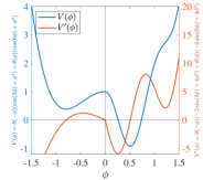
Panel a of Fig.S1 shows the profiles and the derivative of the potential (S1) with . Obviously, the potential satisfies our requirement of the continuous. The minimum values of potential sits at and .
Panel b of Fig.S1 exhibits the time evolutions of the scalar fields. There are respectively three cases for each of them to approach (the upper lines) and (the lower lines) at equilibrium time. The inset plot shows the initial fluctuations of the scalar fields around the top, and then continuously roll down the potential as the arrows indicate.
Panel c of Fig.S1 is the relation between and the ratio . From the potential (S1) we see that , therefore, the relations shown in panel c, i.e., , exactly satisfies our prediction in Eq.(6) in the main text.
Panel d of Fig.S1 shows the relations between and . The linear relation in numerics and theoretical predictions Eq.(5) in the main text match each other very well.
Appendix B Binomial distribution with cosine-type potential
In Fig.S2 we show the counting statistics of the rolling down to the right side with the cosine-type potential in Eq.(S1). For the left column, i.e., Fig.S2 a and c, we set and . Therefore, the probability to roll down to the right side is according to Eq.(6) in the main text. While for the right column, i.e., Fig.S2 b and d, we set and , thus .
From panel a and b of Fig.S2, we can see that for the different probabilities and different trials numbers , the histogram of are consistent with the theoretical binomial distributions in Eq.(12) in the main text very well.
Fig.S2 c and d shows the probability to roll down to the right with zero times in trials, i.e., . Theoretically, from the binomial distribution Eq.(12) in the main text, this probability should be . The two inset plots show the corresponding logarithmic figures, i.e., vs. . Specifically, from the inset plots we can see that the slopes are exactly the value of since . Therefore, from the two plots we see that the numerical statistics match the theoretical predictions very well.