Inflation Models with Correlation and Skew

Orcan Ögetbil111orcan.ogetbil@wellsfargo.com  and Bernhard Hientzsch222bernhard.hientzsch@wellsfargo.com
Corporate Model Risk, Wells Fargo Bank
Abstract

We formulate a forward inflation index model with multi-factor volatility structure featuring a parametric form that allows calibration to correlations between indices of different tenors observed in the market. Assuming the nominal interest rate follows a single factor Gaussian short rate model, we present analytical prices for zero-coupon and year-on-year swaps, caps, and floors. The same method applies to any interest rate model for which one can compute the zero-coupon bond prices and measure shifts. We extend the multi-factor model with leverage functions to capture the entire market volatility skew with a single process. The time-consuming calibration step of this model can be avoided in the simplified model that we further propose. We demonstrate the leveraged and the simplified models with market data.

1 Introduction

The general increase in the prices of goods and services in an economy is referred as inflation. Inflation is usually measured by some consumer price index (CPI), a weighted average of a selected set of goods and services. As inflation has direct impact on purchasing power it constitutes an investment risk, which can be mitigated by inflation-linked securities. The global increase in annual inflation over the past decade has been accompanied by growth in demand for such securities. According to [1], the global inflation-linked bonds market size has grown by 64% to USD 2.82 trillion over the decade leading to April 2023.

The most common instruments traded in the inflation-linked securities market are options on inflation index based zero-coupon and year-on-year swaps. In a zero-coupon swap, the fixed leg payoff at the payment date is computed by annually compounding a target rate $\bar{K}$ to maturity. The floating leg payoff is directly proportional to the inflation index observed at the reset date. The current US and EUR inflation markets exhibit a two to three month lag between inflation index reset and zero-coupon swap payoff dates. In a year-on-year swap, the floating payment depends on the ratio of two inflation index values that are reset one year apart, and the fixed payment is based on a simple target rate $\bar{K}_{Y}$.

Zero-coupon and Year-on-Year Inflation Markets might have different market participants and could well be considered as separate segments of the market with somewhat different factors impacting pricing in each. With sufficient data the two markets can be modeled independently. For example, [2] models the year-on-year market by a quadratic Gaussian process. As an alternative approach [3] builds a framework to calibrate to both markets in a single SABR-like model. While making a modeling choice, a significant concern is data availability. Zero-coupon option data seems to be more readily available than year-on-year option data. While the models we present in this paper can be calibrated to both markets, our focus is calibrating to zero-coupon market; in the mean time the models can price both types of options.

In earlier work, Jarrow and Yildirim considered modeling three processes [4]: real forward rate, nominal forward rate and the CPI, where the drift of the CPI process is the difference between nominal and real interest rates. While this formulation allows pricing of zero-coupon and year-on-year swaps, it relies on unobservable real forward rate data for calibration. Kazziha models inflation rates as discrete forward processes in [5]. In this approach, the forward inflation rate follows log-normal dynamics and is a martingale in the associated forward measure. Log-normal dynamics have been further analyzed in [6] and [7]. Modeling both the short rate and the inflation index with simple Hull-White processes allows closed form solutions [8]. A multi-factor volatility model with SABR-like volatility dynamics with closed form approximations under frozen drift assumptions were formulated by [3]. [9] studies the joint evolution of interest and inflation rates as jump processes in the European market. A Cox-Ingersoll-Ross type stochastic variance process for inflation was introduced in [10], which yields a fast Fourier transform based analytical solution for the uncorrelated case, and an approximation with frozen drift assumption for the correlated case. Extending real and nominal rates modeling approach, [11] proposes a stochastic local volatility model. It however excludes details for calibration steps of leverage functions as well as numerical demonstration.

Our first goal in this paper is to construct a multi-factor log-normal model for inflation index that captures correlations between underliers of different tenors observed in the market. We model the interest rate stochastically by a one factor Gaussian process. While our approach can work with any short rate model as long as certain quantities can be computed, here we demonstrate it with the one factor Gaussian model G1++. We start by reviewing the Kazziha model subject to G1++ interest rate in section 2. Section 3 introduces the zero-coupon and year-on-year swaps, caps and floors under consideration. In section 4, we formulate parametric two and three factor models which capture the market correlations, and present closed form formulae for zero-coupon and year-on-year instruments. Later we extend this model with leverage functions to capture the volatility skew observed in the market. To conclude this section, we further propose a simplified model, which avoids the calibration step required by the leveraged model, and performs similarly well. Finally, section 5 summarizes our findings.

2 Kazziha inflation model under G1++ interest rate

Before proceeding with modeling the inflation we furnish the base environment with a short rate process by which we can compute bond prices. Let $W^{\mathbb{Q}\text{(r)}}$ be a Brownian motion under risk-neutral measure $\mathbb{Q}$ of filtered probability space $\left(\Omega,\mathcal{F},\left\{\mathcal{F}_{t},t\geq 0\right\},\mathbb{Q}\right)$. We assume that the numéraire associated with the risk-neutral measure $\mathbb{Q}$, that is the money market account $B(t)$, accrues at short rate $r(t)$ by $dB(t)=r(t)B(t)dt$. The short rate is modeled by a Gaussian single factor process [12],

$$\begin{split}r_{t}&=x_{t}+\phi_{t},\\ dx_{t}&=-a_{t}x_{t}dt+\sigma^{r}_{t}dW^{\mathbb{Q}\text{(r)}}_{t}.\end{split}$$ (2.1)

Here $\phi_{t}$ is the shift function that is calibrated to market discount curve, $a_{t}\geq 0$ are the mean reversion coefficients, $\sigma^{r}_{t}>0$ are the volatility coefficients, and $x_{0}=0$. The discount factor is given by $D(t)\equiv 1/B(t)=\exp{\left[-\int_{0}^{t}r(u)du\right]}$.

We denote by $P(t,T)\equiv\mathbf{E}^{\mathbb{Q}}\left[\frac{D(T)}{D(t)}\middle|\mathcal{F}_{t}\right]$ the time $t$ value of the zero coupon bond maturing at time $T$, through which we define the instantaneous forward rate

$$f(t,T)\equiv-\frac{\partial\log P(t,T)}{\partial T}=-\frac{1}{P(t,T)}\frac{\partial P(t,T)}{\partial T}.$$ (2.2)

Under the $T$-forward measure $\mathbb{P}^{T}$ defined by the numéraire $P(t,T)$, the short rate process evolves as [13]

$$dx_{t}=\left[-a_{t}x_{t}-b(t,T)(\sigma^{r}_{t})^{2}\right]dt+\sigma^{r}_{t}dW^{\mathbb{P}^{T}\text{(r)}}_{t},$$ (2.3)

with

$$b(t,T)\equiv\int_{t}^{T}e^{-\int_{t}^{v}a_{z}dz}dv.$$

Here $W^{\mathbb{P}^{T}\text{(r)}}$ is a Brownian motion under the $T$-forward measure $\mathbb{P}^{T}$, and it is related to $W^{\mathbb{Q}\text{(r)}}$ by

$$dW^{\mathbb{P}^{T}\text{(r)}}_{t}=dW^{\mathbb{Q}\text{(r)}}_{t}+b(t,T)\sigma^{r}_{t}dt.$$ (2.4)

Using Itô’s lemma one can write the SDEs for the zero coupon bond and the instantaneous forward rate in the risk neutral measure as

$$\begin{split}\frac{dP(t,T)}{P(t,T)}=&r_{t}dt-b(t,T)\sigma^{r}_{t}dW^{\mathbb{Q}\text{(r)}}_{t},\\ df(t,T)=&b(t,T)\frac{\partial b(t,T)}{\partial T}(\sigma^{r}_{t})^{2}dt+\frac{\partial b(t,T)}{\partial T}\sigma^{r}_{t}dW^{\mathbb{Q}\text{(r)}}_{t},\end{split}$$ (2.5)

and in the $T$-forward measure $\mathbb{P}^{T}$ as

$$\begin{split}\frac{dP(t,T)}{P(t,T)}=&\left[r_{t}+\left(b(t,T)\sigma^{r}_{t}\right)^{2}\right]dt-b(t,T)\sigma^{r}_{t}dW^{\mathbb{P}^{T}\text{(r)}}_{t},\\ df(t,T)=&\frac{\partial b(t,T)}{\partial T}\sigma^{r}_{t}dW^{\mathbb{P}^{T}\text{(r)}}_{t}.\end{split}$$ (2.6)

The above zero coupon bond price is solved as

$$\frac{P(t,T)}{P(0,T)}=\exp{\left[\int_{0}^{t}\left(r_{s}+\frac{1}{2}\left(b(s,T)\sigma^{r}_{s}\right)^{2}\right)ds-\int_{0}^{t}b(s,T)\sigma^{r}_{s}dW^{\mathbb{P}^{T}\text{(r)}}_{s}\right]},$$ (2.7)

where $P(0,T)$ is the time-zero market value of the zero coupon bond $P(t,T)$. The time $t$ value of the zero coupon bond price can be written as

$$P(t,T)=\exp\left[-\int_{t}^{T}\left(\phi_{s}-\frac{1}{2}\left(b(s,T)\sigma_{s}^{r}\right)^{2}\right)ds-b(t,T)x_{t}\right]$$ (2.8)

Given a set of time-zero discount factors $P(0,T_{1}),\ldots,P(0,T_{N})$ at times $T_{1},\ldots,T_{N}$ and model parameters $a_{t},\sigma_{t}^{r}$, one can compute the shift function with

$$\phi_{T_{n}}=\frac{1}{T_{n}-T_{n-1}}\log\frac{P^{z}(0,T_{n})P(0,T_{n-1})}{P^{z}(0,T_{n-1})P(0,T_{n})},$$ (2.9)

where

$$P^{z}(t,T)=\exp\left[\frac{1}{2}\int_{t}^{T}\left(b(s,T)\sigma_{s}^{r}\right)^{2}ds-b(t,T)x_{t}\right].$$

Consider a new zero coupon bond $P(t,\bar{T})$ maturing at time $\bar{T}$, with associated $\bar{T}$-forward measure $\mathbb{P}^{\bar{T}}$. The Radon-Nikodym derivative reads

$$\frac{d\mathbb{P}^{\bar{T}}}{d\mathbb{P}^{T}}=\frac{P(t,T)P(0,\bar{T})}{P(t,\bar{T})P(0,T)}.$$

Plugging in (2.7), this derivative becomes

$$\begin{split}\frac{d\mathbb{P}^{\bar{T}}}{d\mathbb{P}^{T}}=\exp\Big{[}&\int_{0}^{t}-\frac{1}{2}(\sigma^{r}_{s})^{2}\left(b^{2}(s,\bar{T})-b^{2}(s,T)\right)ds\\ &-\int_{0}^{t}\sigma^{r}_{s}b(s,\bar{T})dW^{\mathbb{P}^{\bar{T}}\text{(r)}}_{s}+\int_{0}^{t}\sigma^{r}_{s}b(s,T)dW^{\mathbb{P}^{T}\text{(r)}}_{s}\Big{]}.\end{split}$$

By Girsanov theorem, one sees that

$$dW^{\mathbb{P}^{\bar{T}}\text{(r)}}_{t}=dW^{\mathbb{P}^{T}\text{(r)}}_{t}+\sigma^{r}_{t}\left(b(t,\bar{T})-b(t,T)\right)dt$$ (2.10)

is a Brownian motion under $\mathbb{P}^{\bar{T}}$.

Let us denote by $I(t)$ the CPI at time $t$. Consider a single payment fixed-float swap on the CPI. The forward CPI $F(t;T,\tilde{T})$ is defined as the fixed amount to be set at $T$ and exchanged at time $\tilde{T}$ so that the swap has zero value at time $t$.

$$F(t;T,\tilde{T})=E^{\mathbb{P}^{\tilde{T}}}\left[I(T)\arrowvert\mathcal{F}_{t}\right].$$ (2.11)

We define inflation linked zero coupon bond in terms of the nominal bond $P(t,\tilde{T})$ and the forward CPI rate $F(t;T,\tilde{T})$ as

$$P_{\text{IL}}(t,\tilde{T})\equiv P(t,\tilde{T})\cdot F(t;T,\tilde{T}).$$

CPI values are announced at times $T_{i}=T_{0},T_{1},\ldots,T_{I}$. In Kazziha model, the dynamics for $F_{i}(t)\equiv F(t;T_{i},\tilde{T}_{i})$ are specified by the single-factor log-normal process [5]

$$\frac{dF_{i}(t)}{F_{i}(t)}=\sigma_{i}dW^{\mathbb{P}^{\tilde{T}_{i}}\text{(F)}}_{t}$$ (2.12)

where $W^{\mathbb{P}^{\tilde{T}_{i}}\text{(F)}}$ is a Brownian motion under the $\tilde{T}_{i}$-forward measure $\mathbb{P}^{\tilde{T}_{i}}$ with numéraire $P(t,\tilde{T}_{i})$.

To price derivatives involving two or more forward CPIs, one needs a common measure. For this purpose one considers a nominal zero coupon bond $P(t,T_{p})$ of maturity $T_{p}$. Under the measure associated with $P(t,T_{p})$, the CPI process generally has nonzero drift,

$$\frac{dF_{i}(t)}{F_{i}(t)}=\mu_{i}(t)dt+\sigma_{i}dW^{\mathbb{P}^{T_{p}}\text{(F)}}_{t}.$$

Let $\rho_{rF}$ be the coefficient of correlation between the Brownian motions $W^{\mathbb{P}^{T_{p}}\text{(r)}}$ and $W^{\mathbb{P}^{T_{p}}\text{(F)}}$ is $\rho_{rF}=\frac{d}{dt}\left<W^{\mathbb{P}^{T_{p}}\text{(r)}},W^{\mathbb{P}^{T_{p}}\text{(F)}}\right>_{t}$. Using (2.10) and Lemma A.1 of [13], we find that under $\mathbb{P}^{T_{p}}$ the CPI process follows

$$\frac{dF_{i}(t)}{F_{i}(t)}=-\rho_{rF}\sigma_{i}\sigma^{r}_{t}\left(b(t,T_{p})-b(t,\tilde{T}_{i})\right)dt+\sigma_{i}dW^{\mathbb{P}^{T_{p}}\text{(F)}}_{t},$$ (2.13)

so that $\mu_{i}(t)=-\rho_{rF}\sigma_{i}\sigma^{r}_{t}\left(b(t,T_{p})-b(t,\tilde{T}_{i})\right)$. One can use the above SDEs to compute the expectation of the forward CPI as

$$E^{\mathbb{P}^{T_{p}}}\left[F_{i}({T}_{i})\arrowvert\mathcal{F}_{t}\right]=F_{i}(t)e^{\int_{t}^{{T}_{i}}\mu_{i}(s)ds}.$$ (2.14)

Applying the shift in the Brownian motion (2.4) in the reverse direction to the SDE (2.12), or setting $T_{p}=b(t,T_{p})=0$ in (2.13), we obtain the evolution of the CPI process in risk neutral measure

$$\frac{dF_{i}(t)}{F_{i}(t)}=\rho_{rF}\sigma_{i}\sigma^{r}_{t}b(t,\tilde{T}_{i})dt+\sigma_{i}dW^{\mathbb{Q}\text{(F)}}_{t}.$$ (2.15)

3 Inflation Instruments

3.1 Zero-coupon swap, cap, floor

Zero-coupon swaps, caps and floors are the most standard exchange traded instruments. The general swap(let) has a single payoff at time $\tilde{T}_{i}$, that depends on the inflation rate set at time $T_{i}$ as

$$\text{Swap}_{i}=\bar{N}\cdot\left[\frac{I(T_{i})}{\bar{I}}-(1+\bar{K})^{\bar{T}}\right],$$

where $\bar{N}$ is the notional amount, $\bar{I}$ is the reference rate, $\bar{K}$ is the compounded strike, and $\bar{T}$ is the tenor as contractual quantities. Defining $N\equiv\frac{\bar{N}}{\bar{I}}$, and $K\equiv\bar{I}\left(1+\bar{K}\right)^{\bar{T}}$, the payoff can be written as

$$\text{Swap}_{i}(K,\tilde{T}_{i},T_{i},\tilde{T}_{i})=N(I(T_{i})-K).$$ (3.1)

The time $t$ value of this swap can be evaluated analytically as

$$\begin{split}\text{Swap}_{i}(K,t,T_{i},\tilde{T}_{i})=&N\cdot P(t,\tilde{T}_{i})\cdot E^{\mathbb{P}^{\tilde{T}_{i}}}\left[I(T_{i})-K\middle|\mathcal{F}_{t}\right]\\ =&N\cdot P(t,\tilde{T}_{i})\cdot\left[F_{i}(t)-K\right].\end{split}$$ (3.2)

The cap(let) and the floor(let) have a single payoff at time $\tilde{T}_{i}$, that depends on the capped/floored CPI rate set at time $T_{i}$ as

$$\begin{split}\text{Cap}_{i}(K,\tilde{T}_{i},T_{i},\tilde{T}_{i})=&N\cdot\left[I(T_{i})-K\right]^{+},\\ \text{Floor}_{i}(K,\tilde{T}_{i},T_{i},\tilde{T}_{i})=&N\cdot\left[K-I(T_{i})\right]^{+}.\end{split}$$ (3.3)

where the quantities are as defined for the zero coupon swap. The time $t$ value of the cap and the floor are given by

$$\begin{split}\text{Cap}_{i}(K,t,T_{i},\tilde{T}_{i})=&N\cdot P(t,\tilde{T}_{i})\cdot E^{\mathbb{P}^{\tilde{T}_{i}}}\left[\left(I(T_{i})-K\right)^{+}\middle|\mathcal{F}_{t}\right],\\ =&N\cdot P(t,\tilde{T}_{i})\cdot\left[F_{i}(t)\Phi(d_{1})-K\Phi(d_{2})\right],\\ \text{Floor}_{i}(K,t,T_{i},\tilde{T}_{i})=&N\cdot P(t,\tilde{T}_{i})\cdot E^{\mathbb{P}^{\tilde{T}_{i}}}\left[\left(K-I(T_{i})\right)^{+}\middle|\mathcal{F}_{t}\right].\\ =&N\cdot P(t,\tilde{T}_{i})\cdot\left[K\Phi(-d_{2})-F_{i}(t)\Phi(-d_{1})\right],\end{split}$$ (3.4)

where $d_{1}\equiv\frac{1}{\sigma_{i}\sqrt{\tau_{i}}}\log\left(\frac{F_{i}(t)}{K}\right)+\frac{\sigma_{i}\sqrt{\tau_{i}}}{2}$, $d_{2}\equiv d_{1}-\sigma_{i}\sqrt{\tau_{i}}$, $\tau_{i}\equiv T_{i}-t$, $\Phi(\cdot)$ is the cumulative Gaussian probability distribution, the Kazziha parameter $\sigma_{i}$ corresponds to the market volatility $\Sigma_{i}(K)$ for strike $K$ and maturity $T_{i}$, and the zero coupon bond price $P(t,\tilde{T}_{i})$ is given in (2.8).

3.2 Year-on-year swap, cap, floor

The year-on-year inflation swap(let) has a single payoff at time $T_{p}$, that depends on the inflation rates set at time $T_{i}$ and $T_{j}$, with $t<T_{i}<T_{j}<T_{p}$ as

$$\text{YOYSwap}_{i}(K,T_{p},T_{i},T_{j},T_{p})=N\cdot\left[\frac{I(T_{j})}{I(T_{i})}-(1+\bar{K}_{Y})\right],$$ (3.5)

where $N$ is the notional amount, and $\bar{K}_{Y}$ is the strike as contractual quantities. $T_{j}$ is $T_{i}$ plus one year. The time $t$ value of this swap is given by

$$\begin{split}\text{YOYSwap}_{i}(K_{Y},t,T_{i},T_{j},T_{p})=&N\cdot P(t,T_{p})\cdot E^{\mathbb{P}^{T_{p}}}\left[\frac{I(T_{j})}{I(T_{i})}-K_{Y}\middle|\mathcal{F}_{t}\right]\\ =&N\cdot P(t,T_{p})\cdot\left[X_{ij}(t)-K_{Y}\right],\end{split}$$ (3.6)

with $K_{Y}\equiv 1+\bar{K}_{Y}$. The expectation of the forward ratio $X_{ij}(t)\equiv E^{\mathbb{P}^{T_{p}}}\left[\frac{I(T_{j})}{I(T_{i})}\middle|\mathcal{F}_{t}\right]$ is calculated as

$$X_{ij}(t)=\frac{F_{j}(t)}{F_{i}(t)}\exp\left[\int_{t}^{T_{j}}\sigma_{j}\bar{\nu}_{j}(s)ds-\int_{t}^{T_{i}}\sigma_{i}\bar{\nu}_{i}(s)ds-\left(\sigma_{i}\sigma_{j}+\sigma_{i}^{2}\right)(T_{i}-t)\right],$$ (3.7)

and

$$\bar{\nu}_{i}(t)\equiv\rho_{rF}\sigma^{r}_{t}\left(b(t,\tilde{T}_{i})-b(t,T_{p})\right).$$

The year-on-year cap(let) and the floor(let) have a single payoff at time $T_{p}$, that depends on the capped/floored inflation rates set at times $T_{i}$ and $T_{j}$ as

$$\begin{split}\text{YOYCap}_{i}(K_{Y},T_{p},T_{i},T_{j},T_{p})=&N\cdot\left[\frac{I(T_{j})}{I(T_{i})}-K_{Y}\right]^{+},\\ \text{YOYFloor}_{i}(K_{Y},T_{p},T_{i},T_{j},T_{p})=&N\cdot\left[K_{Y}-\frac{I(T_{j})}{I(T_{i})}\right]^{+},\end{split}$$ (3.8)

where the quantities are as defined for the year-on-year swap. The time $t$ value of the cap and the floor are computed analytically as

$$\begin{split}\text{YOYCap}_{i}(K_{Y},t,T_{i},T_{j},T_{p})&=N\cdot P(t,T_{p})\cdot E^{\mathbb{P}^{T_{p}}}\left[\left(\frac{I(T_{j})}{I(T_{i})}-K_{Y}\right)^{+}\middle|\mathcal{F}_{t}\right],\\ &=N\cdot P(t,T_{p})\cdot\left[X_{ij}(t)\Phi(d_{1})-K_{Y}\Phi(d_{2})\right],\\ \text{YOYFloor}_{i}(K_{Y},t,T_{i},T_{j},T_{p})&=N\cdot P(t,T_{p})\cdot E^{\mathbb{P}^{T_{p}}}\left[\left(K_{Y}-\frac{I(T_{j})}{I(T_{i})}\right)^{+}\middle|\mathcal{F}_{t}\right].\\ &=N\cdot P(t,T_{p})\cdot\left[K_{Y}\Phi(-d_{2})-X_{ij}(t)\Phi(-d_{1})\right],\end{split}$$ (3.9)

with

$$\begin{split}d_{1}\equiv&\frac{\log\left(\frac{X_{ij}(t)}{K_{Y}}\right)}{\sqrt{\eta_{ij}(t)}}+\frac{1}{2}\sqrt{\eta_{ij}(t)},\\ d_{2}\equiv&d_{1}-\sqrt{\eta_{ij}(t)},\\ \eta_{ij}(t)\equiv&\sigma_{j}^{2}(T_{j}-t)+\left(\sigma_{i}^{2}-2\sigma_{i}\sigma_{j}\right)(T_{i}-t).\\ \end{split}$$

4 Multi-factor models

4.1 Imperfect Correlations

A significant drawback of the model (2.12) is that it is driven by a single Brownian factor, so that it implies perfect correlation of swap rate returns between different maturities. We investigate the number of random factors needed by a model to make it consistent with market correlation behavior by doing principal component analysis (PCA) on the daily changes of swap rates, specifically of $X_{k}(t)\equiv\log F_{k}(t)$ where the index denotes the $k$th nearest maturity after calendar time $t$. PCA results are summarized in Figure 4.1. We see that 71%, 86% and 75% of the variations in curve movements are explained by a single factor for USD, EUR, and GBP respectively. The numbers go over 89%, 97%, and 94% with two factors, and over 95%, 99%, and 98% with three factors.

Refer to caption
Refer to caption
Refer to caption
Figure 4.1: First three eigenvectors computed by PCA on daily returns of $X_{k}(t)$. We used historical daily closing values between 2020-03-01 and 2023-01-23 for USD, and between 2019-11-11 and 2022-11-08 for EUR and GBP inflation.

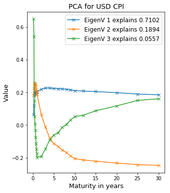
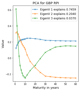
We observe that the PCA yielded similar eigenvectors for the three inflation curves considered. The first eigenvector is nearly constant through maturity whereas the second and third eigenvectors contain twists that generate the imperfect correlations. Motivated by this analysis, we decide to formulate a model in $\tilde{T}_{i}$-forward measure $\mathbb{P}^{\tilde{T}_{i}}$ with $M$ independent random factors $W^{\mathbb{P}^{\tilde{T}_{i}}(F^{\alpha})},\alpha\in\{1,\ldots,M\}$ and parameters $\mathcal{P}_{M}$ to incorporate imperfect market correlations between different maturites in the inflation curve,

$$\frac{dF_{i}(t)}{F_{i}(t)}=\sigma_{i}\sum_{\alpha=1}^{M}\lambda_{i}^{\alpha}(t)dW^{\mathbb{P}^{\tilde{T}_{i}}(F^{\alpha})}_{t},$$ (4.1)

with Kazziha parameter $\sigma_{i}$. For $M=1$ and $\lambda_{i}^{1}(t)=1$ this corresponds to the Kazziha model. For a two factor model setup, $M=2$, we write

$$\begin{split}\lambda_{i}^{1}(t)=&1,\\ \lambda_{i}^{2}(t)=&h_{1}e^{-\kappa(T_{i}-t)}+h_{2},\end{split}$$ (4.2)

with model parameters $\mathcal{P}_{2}=\{h_{1},h_{2},\kappa\}$, and $\kappa>0$; and for three factors, $M=3$, we extend this as

$$\begin{split}\lambda_{i}^{1}(t)=&1,\\ \lambda_{i}^{2}(t)=&h_{1}e^{-\kappa_{1}(T_{i}-t)}+h_{2},\\ \lambda_{i}^{3}(t)=&h_{3}(T_{i}-t)e^{-\kappa_{2}(T_{i}-t)}+h_{4},\end{split}$$ (4.3)

with model parameters $\mathcal{P}_{3}=\{h_{1},h_{2},h_{3},h_{4},\kappa_{1},\kappa_{2}\}$, and $\kappa_{1},\kappa_{2}>0$. The multifactor model implies the following instantaneous correlation at time $t$ between different tenors of the inflation curve,

$$\rho^{M}(t,T_{i},T_{j})=\text{corr}\left(d\log F_{i}(t),d\log F_{j}(t)\right)=\frac{\zeta_{ij}^{M}(t)}{\sqrt{\zeta^{M}_{ii}(t)\zeta^{M}_{jj}(t)}},$$ (4.4)

where we defined

$$\zeta^{M}_{ij}(t)\equiv{\sum_{\alpha=1}^{M}\lambda_{i}^{\alpha}(t)\lambda_{j}^{\alpha}(t)}.$$ (4.5)

We note that $\zeta^{1}_{ij}(t)=1$ for the Kazziha model. For a better fit to historical correlation behavior, one can obtain market correlations $\rho_{\text{market}}(T_{j},T_{k})$ from historical data series and then minimize the objective function333This correlation matching methodology was introduced in [14] for commodity underliers. Here we apply the idea to inflation index underliers.

$$J(\mathcal{P}_{M})=\sum_{j=0}^{I}\sum_{k=j}^{I}\left[\rho^{M}(0,T_{j},T_{k})-\rho_{\text{market}}(T_{j},T_{k})\right]^{2}.$$ (4.6)

Having a set of calibrated parameters $\mathcal{P}_{M}$, $\sigma_{i}$ remains the last parameter to determine. The total variance is computed by integrating the log-variance of the process (4.1) over the lifetime of the option. Setting the model total implied variance to the variance implied by the market allows the model to produce market prices. In practice, one typically sets $\sigma_{i}$ to match market volatilities $\Sigma_{i}$; for example at-the-money volatilities, or volatilities corresponding to a target strike,

$$w^{M}_{i}(t)\equiv\Sigma_{i}^{2}(T_{i}-t)=\sigma_{i}^{2}\int_{t}^{T_{i}}\zeta^{M}_{ii}(s)ds.$$ (4.7)

The integral on the right hand side can be solved explicitly for the two-factor model (4.2) as

$$\int_{t}^{T_{i}}\zeta^{2}_{ii}(s)ds=(1+h_{2}^{2})\tau_{i}+\frac{h_{1}^{2}}{2\kappa}\left(1-e^{-2\kappa\tau_{i}}\right)+\frac{2h_{1}h_{2}}{\kappa}\left(1-e^{-\kappa\tau_{i}}\right),$$

and for the three-factor model (4.3) as

$$\begin{split}\int_{t}^{T_{i}}\zeta^{3}_{ii}(s)ds=&(1+h_{2}^{2}+h_{4}^{2})\tau_{i}+\frac{h_{1}^{2}}{2\kappa_{1}}\left(1-e^{-2\kappa_{1}\tau_{i}}\right)+\frac{2h_{1}h_{2}}{\kappa_{1}}\left(1-e^{-\kappa_{1}\tau_{i}}\right)\\ &-\frac{h_{3}^{2}\tau_{i}}{2\kappa_{2}^{2}}(\kappa_{2}\tau_{i}+1)e^{-2\kappa_{2}\tau_{i}}-\frac{2h_{3}h_{4}\tau_{i}}{\kappa_{2}}e^{-\kappa_{2}\tau_{i}}\\ &+\frac{h_{3}^{2}}{4\kappa_{2}^{3}}\left(1-e^{-2\kappa_{2}\tau_{i}}\right)+\frac{2h_{3}h_{4}}{\kappa_{2}^{2}}\left(1-e^{-\kappa_{2}\tau_{i}}\right),\end{split}$$

with time to maturity $\tau_{i}\equiv T_{i}-t$.

The cap and floor prices have the analytical solutions

$$\begin{split}\text{Cap}_{i}(K,t,T_{i})&=N\cdot P(t,\tilde{T}_{i})\cdot\left[F_{i}(t)\Phi(d_{1})-K\Phi(d_{2})\right],\\ \text{Floor}_{i}(K,t,T_{i})&=N\cdot P(t,\tilde{T}_{i})\cdot\left[K\Phi(-d_{2})-F_{i}(t)\Phi(-d_{1})\right],\end{split}$$ (4.8)

with

$$\begin{split}d_{1}\equiv&\frac{\log\left(\frac{F_{i}(t)}{K}\right)}{\sqrt{w^{M}_{i}(t)}}+\frac{1}{2}\sqrt{w^{M}_{i}(t)},\\ d_{2}\equiv&d_{1}-\sqrt{w^{M}_{i}(t)},\\ \end{split}$$

The year-on-year cap and floor prices have the analytical solutions

$$\begin{split}\text{YOYCap}_{i}(K_{Y},t,T_{i},T_{j},T_{p})&=N\cdot P(t,T_{p})\cdot\left[X_{ij}(t)\Phi(d_{1})-K_{Y}\Phi(d_{2})\right],\\ \text{YOYFloor}_{i}(K_{Y},t,T_{i},T_{j},T_{p})&=N\cdot P(t,T_{p})\cdot\left[K_{Y}\Phi(-d_{2})-X_{ij}(t)\Phi(-d_{1})\right],\end{split}$$ (4.9)

with

$$\begin{split}X_{ij}(t)\equiv&\frac{F_{j}(t)}{F_{i}(t)}\exp\left[\int_{t}^{T_{j}}\sigma_{j}\bar{\nu}^{M}_{j}(s)ds-\int_{t}^{T_{i}}\left(\sigma_{i}\bar{\nu}^{M}_{i}(s)-\sigma_{i}\sigma_{j}\zeta^{M}_{ij}(s)-\sigma_{i}^{2}\zeta^{M}_{ii}(s)\right)ds\right],\\ d_{1}\equiv&\frac{\log\left(\frac{X_{ij}(t)}{K_{Y}}\right)}{\sqrt{\eta^{M}_{ij}(t)}}+\frac{1}{2}\sqrt{\eta^{M}_{ij}(t)},\\ d_{2}\equiv&d_{1}-\sqrt{\eta^{M}_{ij}(t)},\\ \bar{\nu}^{M}_{i}(t)\equiv&\sigma^{r}_{t}\left(b(t,\tilde{T}_{i})-b(t,T_{p})\right)\sum_{\alpha=1}^{M}\rho_{rF^{\alpha}}\lambda_{i}^{\alpha}(t).\\ \end{split}$$

The implied variance $\eta^{M}_{ij}(t)$ of the year-on-year forward ratio can be written in terms of model parameters as

$$\begin{split}\eta^{M}_{ij}(t)\equiv&\int_{t}^{T_{j}}\sigma_{j}^{2}\zeta^{M}_{jj}(s)ds+\int_{t}^{T_{i}}\left(\sigma_{i}^{2}\zeta^{M}_{ii}(s)-2\sigma_{i}\sigma_{j}\zeta^{M}_{ij}(s)\right)ds.\\ =&w^{M}_{j}(t)+w^{M}_{i}(t)-2\sigma_{i}\sigma_{j}\int_{t}^{T_{i}}\zeta^{M}_{ij}(s)ds.\\ \end{split}$$

In the ideal case broker quotes are available for options on the year-on-year forward ratio $\frac{I(T_{j})}{I(T_{i})}$, one can calibrate the model parameters $\sigma_{i}$ to fit the quotes. In the absence of such quotes, once can use the $\sigma_{i}$s from regular cap-floors. In this case, however, the moneyness to choose for each individual underlier $F_{i}(t)$ and $F_{j}(t)$ will have significant impact on the year-on-year price. We will investigate this issue in subsection 4.4.

Before moving on we write down the evolution of the multi-factor model (4.1) in the risk neutral measure $\mathbb{Q}$ as

$$\frac{dF_{i}(t)}{F_{i}(t)}=\sigma_{i}\nu^{M}_{i}(t)dt+\sigma_{i}\sum_{\alpha=1}^{M}\lambda_{i}^{\alpha}(t)dW^{\mathbb{Q}(F^{\alpha})}_{t},$$ (4.10)

where

$$\nu^{M}_{i}(t)\equiv\sigma^{r}_{t}b(t,\tilde{T}_{i})\sum_{\alpha=1}^{M}\rho_{rF^{\alpha}}\lambda_{i}^{\alpha}(t).$$ (4.11)

4.1.1 Calibration Example

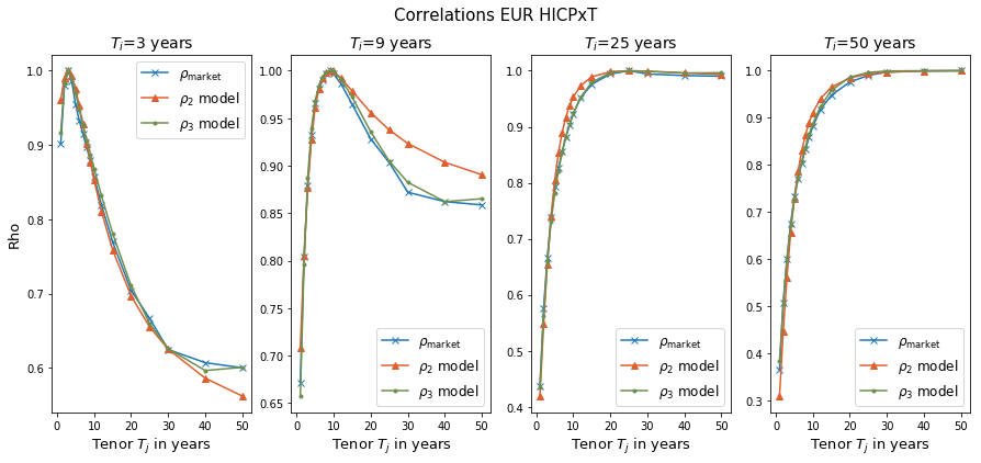
We calibrate the two and three factor models (4.2) and (4.3) to historical data using scipy’s L-BFGS-B optimizer on the objective function (4.6). Figure 4.2 compares the correlations implied by the two and three factor models to historical market correlations. The two factor model seems to capture most of the historical market correlation behavior, and evidently the three factor model provides some additional improvement.

Refer to caption
Figure 4.2: Market correlations and correlations implied by two and three factor models for several $T_{i}$s as a function of $T_{j}$. Market correlations were computing using historical daily closing values between 2019-11-11 and 2022-11-08 for EUR inflation.

For the two factor model the best fitting parameters are found to be $\mathcal{P}_{2}=\{h_{1},h_{2},\kappa\}=\{-3.689,\ 3.553,\ 0.042\}$, whereas for the three factor model they are $\mathcal{P}_{3}=\{h_{1},h_{2},h_{3},h_{4},\kappa_{1},\kappa_{2}\}=\{2.319,\ -2.068,\ 0.275,\ -0.145,$ $0.085,\ 0.142\}.$

Table 4.1 lists the market quotes for the volatilities at various tenors and strikes for EUR inflation index HICPxT as of 2023-04-28.

$\bar{K}$
$T_{i}$ $F_{i}(0)$ -0.02 -0.01 0.00 0.01 0.02 0.03 0.04 0.05
1 124.43 3.101% 2.756% 2.442% 2.189% 1.974% 1.839% 1.841% 1.969%
2 127.26 2.523% 2.242% 1.987% 1.781% 1.409% 1.293% 1.587% 1.971%
5 136.30 3.620% 3.218% 2.851% 2.556% 2.243% 2.415% 2.915% 3.471%
7 142.97 4.152% 3.691% 3.270% 2.931% 2.755% 2.986% 3.466% 4.005%
10 153.93 4.991% 4.437% 3.931% 3.523% 3.493% 3.789% 4.273% 4.817%
12 162.04 5.494% 4.884% 4.327% 3.878% 3.929% 4.253% 4.735% 5.273%
15 175.83 6.043% 5.371% 4.759% 4.265% 4.393% 4.735% 5.206% 5.729%
20 201.50 7.102% 6.313% 5.593% 5.013% 5.203% 5.548% 6.008% 6.525%
Table 4.1: Market volatility quotes $\Sigma_{i}(K)$ for various tenors $\bar{T}=T_{i}$ and strikes $\bar{K}$ with $K=F_{i}(0)\left(1+\bar{K}\right)^{\bar{T}}$ for EUR inflation index HICPxT. Time is given in years.

We compute the volatility factors $\sigma_{i}$ by using at-the-money ($\bar{K}=0$) market volatilities in (4.7) and list them in Table 4.2.

$\sigma_{i}$
$T_{i}$ (years) $M=1$ $M=2$ $M=3$
1 0.02925 0.02916 0.02404
2 0.02178 0.02170 0.01952
5 0.02961 0.02836 0.02595
7 0.03360 0.03070 0.02795
10 0.04007 0.03363 0.03091
12 0.04396 0.03477 0.03245
15 0.04820 0.03496 0.03357
20 0.05647 0.03598 0.03634
Table 4.2: Inflation volatility factors $\sigma_{i}$ calibrated for the 1, 2 and 3 factor models (4.1)

4.2 Leverage functions

The multi-factor model we introduced in the last subsection aims to capture cross-tenor correlations as well as market volatilities for a target strike. In order to capture the market volatility smile, that is to reprice market quotes of different strikes, we extend the model (4.1) with unique leverage functions $L_{i}$ for each tenor,

$$\frac{dF_{i}(t)}{F_{i}(t)}=L_{i}(F_{i}(t),t)\sum_{\alpha=1}^{M}\lambda_{i}^{\alpha}(t)dW^{\mathbb{P}^{\tilde{T}_{i}}(F^{\alpha})}_{t}.$$ (4.12)

This model evolves in the risk neutral measure $\mathbb{Q}$ as

$$\frac{dF_{i}(t)}{F_{i}(t)}=\nu^{M}_{i}(t)L_{i}(F_{i}(t),t)dt+L_{i}(F_{i}(t),t)\sum_{\alpha=1}^{M}\lambda_{i}^{\alpha}(t)dW^{\mathbb{Q}(F^{\alpha})}_{t},$$ (4.13)

where $\nu^{M}_{i}(t)$ is defined as in (4.11). The leverage functions are to be calibrated to market quotes. They are related to time-zero prices of $T$-maturity cap(let)s paying (3.3) at time $\tilde{T}_{i}\geq T$ by the Dupire equation [15],

$$L_{i}(K,T)^{2}=\frac{\frac{\partial\text{Cap}_{i}(K,0,T,\tilde{T}_{i})}{\partial T}+\theta_{i}^{\text{Cap}}(K,T)}{\frac{1}{2}K^{2}\frac{\partial^{2}\text{Cap}_{i}(K,0,T,\tilde{T}_{i})}{\partial K^{2}}\zeta^{M}_{ii}(T)},$$ (4.14)

where

$$\begin{split}\theta_{i}^{\text{Cap}}(K,T)\equiv&N\mathbf{E}^{\mathbb{Q}}\left[D(\tilde{T}_{i})\left\{\left[F_{i}(T)-K\right]r_{T}-\nu^{M}_{i}(T)L_{i}(F_{i}(T),T)F_{i}(T)\right\}\mathds{1}_{F_{i}(T)>K}\right]\\ &-f(0,T)\text{Cap}_{i}(K,0,T,\tilde{T}_{i}).\end{split}$$

In terms of floor(let)s with payoff (3.3), the leverage functions are,

$$L_{i}(K,T)^{2}=\frac{\frac{\partial\text{Floor}_{i}(K,0,T,\tilde{T}_{i})}{\partial T}+\theta_{i}^{\text{Floor}}(K,T)}{\frac{1}{2}K^{2}\frac{\partial^{2}\text{Floor}_{i}(K,0,T,\tilde{T}_{i})}{\partial K^{2}}\zeta^{M}_{ii}(T)},$$ (4.15)

where

$$\begin{split}\theta_{i}^{\text{Floor}}(K,T)\equiv&N\mathbf{E}^{\mathbb{Q}}\left[D(\tilde{T}_{i})\left\{\left[K-F_{i}(T)\right]r_{T}+\nu^{M}_{i}(T)L_{i}(F_{i}(T),T)F_{i}(T)\right\}\mathds{1}_{F_{i}(T)<K}\right]\\ &-f(0,T)\text{Floor}_{i}(K,0,T,\tilde{T}_{i}).\end{split}$$

The time-zero price function for a time-$T$ maturity caplet with underlier $F_{i}$ that pays at time $\tilde{T}_{i}$ can be parametrized in terms of log-moneyness $y=\log\frac{K}{F_{i}(0)}$ and the total implied variance $w_{i}$ as [16]

$$\text{Cap}_{i}(y,w_{i})=NP(0,\tilde{T}_{i})F_{i}(0)\left[\Phi(d_{1})-e^{y}\Phi(d_{2})\right]$$ (4.16)

where $d_{1}=-yw_{i}^{-\frac{1}{2}}+\frac{1}{2}w_{i}^{\frac{1}{2}}$, and $d_{2}=d_{1}-w_{i}^{\frac{1}{2}}$. In the total implied variance parametrization, the Dupire equation 4.14 can be casted to $\bar{L}_{i}(y,T)=L_{i}(F_{i}(0)e^{y},T)$ as [15],

$$\bar{L}_{i}(y,T)^{2}=\frac{\frac{\partial\text{Cap}_{i}}{\partial w_{i}}\frac{\partial w_{i}}{\partial T}+\theta^{\text{Cap}}_{i}(F_{i}(0)e^{y},T)}{\frac{\partial\text{Cap}_{i}}{\partial w_{i}}\left[1-\frac{y}{w_{i}}\frac{\partial w_{i}}{\partial y}+\frac{1}{2}\frac{\partial^{2}w_{i}}{\partial y^{2}}+\frac{1}{4}\left(\frac{\partial w_{i}}{\partial y}\right)^{2}\left(-\frac{1}{4}-\frac{1}{w_{i}}+\frac{y^{2}}{w_{i}^{2}}\right)\right]\zeta^{M}_{ii}(T)},$$ (4.17)

with

$$\frac{\partial\text{Cap}_{i}}{\partial w_{i}}=\frac{1}{2}NP(0,\tilde{T}_{i})F_{i}(0)e^{y}\Phi^{\prime}(d_{2})w_{i}^{-\frac{1}{2}}.$$

Similary, the time-zero price function for a time-$T$ maturity floorlet underlier $F_{i}$ that pays at time $\tilde{T}_{i}$ can be parametrized as

$$\text{Floor}_{i}(y,w_{i})=NP(0,\tilde{T}_{i})F_{i}(0)\left[-\Phi(-d_{1})+e^{y}\Phi(-d_{2})\right].$$ (4.18)

In the total implied variance parametrization, the Dupire equation becomes

$$\bar{L}_{i}(y,T)^{2}=\frac{\frac{\partial\text{Floor}_{i}}{\partial w_{i}}\frac{\partial w_{i}}{\partial T}+\theta^{\text{Floor}}_{i}(F_{i}(0)e^{y},T)}{\frac{\partial\text{Floor}_{i}}{\partial w_{i}}\left[1-\frac{y}{w_{i}}\frac{\partial w_{i}}{\partial y}+\frac{1}{2}\frac{\partial^{2}w_{i}}{\partial y^{2}}+\frac{1}{4}\left(\frac{\partial w_{i}}{\partial y}\right)^{2}\left(-\frac{1}{4}-\frac{1}{w_{i}}+\frac{y^{2}}{w_{i}^{2}}\right)\right]\zeta^{M}_{ii}(T)},$$ (4.19)

with

$$\frac{\partial\text{Floor}_{i}}{\partial w_{i}}=\frac{1}{2}NP(0,\tilde{T}_{i})F_{i}(0)e^{y}\Phi^{\prime}(-d_{2})w_{i}^{-\frac{1}{2}}.$$

In the limit the interest rate volatility $\sigma^{r}_{t}$ approaches zero one has $\nu^{M}_{i}(t)=\theta^{\text{Cap}}_{i}=\theta^{\text{Floor}}_{i}=0$, and the expression for the leverage function simplifies to

$$\bar{L}^{s}_{i}(y,T){}^{2}=\frac{\frac{\partial w_{i}}{\partial T}}{\left[1-\frac{y}{w_{i}}\frac{\partial w_{i}}{\partial y}+\frac{1}{2}\frac{\partial^{2}w_{i}}{\partial y^{2}}+\frac{1}{4}\left(\frac{\partial w_{i}}{\partial y}\right)^{2}\left(-\frac{1}{4}-\frac{1}{w_{i}}+\frac{y^{2}}{w_{i}^{2}}\right)\right]\zeta^{M}_{ii}(T)}.$$ (4.20)

We use this expression in the calibration routine below for computing the leverage function at time $t$ close to initial time, where the interest rate is observed at a fixed value.

Inflation options traded on the market written on $F_{i}$ typically have a single maturity $T_{i}$. Accordingly, the market implied volatility $\Sigma_{i}(K)$ for strike $K$ yields a total implied variance $\Sigma_{i}(K)^{2}T_{i}$ at maturity $T_{i}$. Here we make the assumption that the total implied variance accumulates linearly in time as $w_{i}=\Sigma_{i}(K)^{2}T$ for times $T\leq T_{i}$,

$$w_{i}(y,T)=\Sigma_{i}(F_{i}(0)e^{y})^{2}T.$$ (4.21)

We adapt the calibration approach proposed in [13] to compute the leverage functions $\bar{L}_{i}$ for every underlier $F_{i}$ simultaneously time slice by time slice. We perform a Monte Carlo simulation to estimate the expectation appearing in the expressions for $\theta_{i}^{\text{Cap}}(K,T)$ and $\theta_{i}^{\text{Floor}}(K,T)$.

Inputs for calibration

Our calibration routine expects the following quantities as input for leverage function calibration:

  • A multi-factor model (4.1) with parameters calibrated to market data

  • Market CPI rates $F_{i}(0)$ as of the valuation time $t=0$

  • Market implied volatility $\Sigma_{i}(K)$ for each maturity

  • Market yield curve $P(0,T)$

  • G1++ short rate model (2.1) (or any rate model for which one can compute the zero-coupon bond price and the measure shift terms) with parameters calibrated to market data.

  • Coefficients of correlation between the Brownian motions of the short rate and the multi-factor inflation models

Steps for calibration

We calibrate the leverage functions time slice by time slice, in a bootstrapping fashion. Let $t_{k};k=1,\ldots,n$ be the increasing sequence of (positive) times where we will perform the calibration.

  1. 1.

    Using the market implied volatilities $\Sigma_{i}(K)=\Sigma_{i}(F_{i}(0)e^{y})$, generate a total implied variance surface $w_{i}(y,T)$ interpolator. The interpolator must be able to compute the partial derivatives appearing in the local volatility expressions.

  2. 2.

    For the first time slice $t_{1}$, evaluate the simplified equation (4.20) to compute the leverage function values $\bar{L}_{i}(y,t_{1})$ for a predetermined range of strikes for every $i$. This step requires no Monte Carlo simulation. As a result, obtain leverage function values to be used until time $t_{2}$ in the subsequent calibration steps.

  3. 3.

    For each of the subsequent time slices $t_{k},k>1$, Simulate the SDE system (4.1), (2.1) up to time $t_{k}$. By choosing out-of-money options for a predetermined grid of strikes, that is caps for $y>0$ and floors for $y<0$, compute the Monte Carlo estimate for the expectation appearing in (4.2) or (4.2) for every $i$. Obtain the leverage function values $\bar{L}_{i}(y,t_{k})$ from these equations. These values will be used during subsequent simulation steps from time $t_{k}$ to time $t_{k+1}$. This step is first performed with $k=2$ and is then repeated for the remaining time slices.

4.2.1 Calibration Example

We calibrate the multifactor model to market data as of 2023-04-28. We use the same multifactor model parameters we estimated in subsection 4.1.1, and the same volatility data from Table 4.1. For simplicity we ignore the market lag, as is common in the examples in the literature, such that $T_{i}=\tilde{T}_{i}\ \forall i$. The G1++ model parameters are fit to market interest rate swaptions. Here we do not go into details of this fitting. Instead we list the parameters that we use as input, and refer to [17] for calibration of Hull-White-type models with time-dependent parameters. G1++ mean reversion is set to be constant, $a_{t}=0.02$. The market discount curve and G1++ volatility parameters are given in Table 4.3.

$T$ (years) $P(0,T)$
0 1
1 0.9656
2 0.9379
5 0.8706
7 0.8264
10 0.7596
12 0.7152
15 0.6547
20 0.5800
$t$ (years) $\sigma^{r}_{t}$
1 1.071%
2 1.093%
3 0.992%
5 0.839%
10 0.686%
20 0.683%
Table 4.3: Discount factors $P(0,T)$ and G1++ model volatility $\sigma^{r}_{t}$.

The coefficient of correlation between the Brownian motions $W^{\mathbb{Q}(r)}$ and $W^{\mathbb{Q}(F^{\alpha})}$ is $\rho_{rF^{\alpha}}=\frac{d}{dt}\left<W^{\mathbb{Q}(r)},W^{\mathbb{Q}(F^{\alpha})}\right>_{t}=-0.5\ \forall\alpha$.

The leverage functions strike grid is chosen to cover regions of concern. In our implementation, we construct a uniform grid for $\bar{K}$ between -0.02 and 0.05 with spacing 0.001. This is translated to log-moneyness as $y=\bar{T}\log(1+\bar{K})$ for contractual maturity $\bar{T}$. It is important that the chosen grid is covered by the implied volatility data. For the maturity coordinate we first construct a time grid with uniform spacing, e.g. $t_{k+1}-t_{k}=1/4$ until the latest maturity, and then we add the quoted option maturity times to this grid. The expectation in the leverage equation is estimated by simulating 2000 paths and computing Monte Carlo averages of the argument of the expectation.

We simulate the calibrated model over 2000 paths to price caps at various maturities and strikes. The leverage function values are interpolated piecewise linearly in both dimensions during simulation. We invert the pricing formula (4.8) to compute the model implied volatilities from the Monte Carlo price means, as well as price means bumped by two Monte Carlo standard errors in both directions. Figure 4.3 shows that the market implied volatilities are within two Monte Carlo errors of the simulation means for most strikes within the test range.

Refer to caption
Figure 4.3: Market and Monte Carlo implied volatilities for the leveraged model (4.12) with $M=3$ factors (4.3) for EUR inflation as of 2023-04-28. The market implied volatilities are within two Monte Carlo standard errors (blue shaded regions) for most strikes.

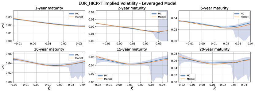
This test demonstrates that the implementation of the leveraged three factor model recovers market quotes at various strikes and maturities.

4.3 Simplified Model

The leveraged model of the previous subsection seems to capture the market skew for caps and floors well. The calibration routine of the leverage function, however, involves a Monte Carlo estimation. Here we formulate a simplified model by ignoring negligible terms in the Dupire equation such that the resulting model does not require the calibration step.

We can approximate the leverage function by

$$\bar{L}_{i}(y,T)^{2}\approx\Lambda_{i}(y,T)^{2}\equiv\frac{\frac{\partial w_{i}}{\partial T}}{\left[1-\frac{1}{2}\frac{y}{w_{i}}\frac{\partial w_{i}}{\partial y}\right]^{2}\zeta^{M}_{ii}(T)}.$$ (4.22)

By plugging in the expression (4.21) for total implied variance, (4.22) can be written as

$$\Lambda_{i}(y,T)=\frac{q_{i}(F_{i}(0)e^{y})}{\sqrt{\zeta^{M}_{ii}(T)}},$$ (4.23)

where

$$q_{i}(K)\equiv\frac{\Sigma_{i}(K)}{1-\frac{K\log{\frac{K}{F_{i}(0)}}}{\Sigma_{i}(K)}\frac{\partial\Sigma_{i}}{\partial K}}.$$ (4.24)

With this function, we can formulate a simplified multi-factor model as

$$\frac{dF_{i}(t)}{F_{i}(t)}=\frac{q_{i}(F_{i}(t))}{\sqrt{\zeta^{M}_{ii}(t)}}\sum_{\alpha=1}^{M}\lambda_{i}^{\alpha}(t)dW^{\mathbb{P}^{\tilde{T}_{i}}(F^{\alpha})}_{t}.$$ (4.25)

In practice we use an algorithmic cap parameter $\eta$ for $q_{i}(K)$,

$$q_{i}(K)\equiv\frac{\Sigma_{i}(K)}{\max\left(\frac{1}{\eta},1-\frac{K\log{\frac{K}{F_{i}(0)}}}{\Sigma_{i}(K)}\frac{\partial\Sigma_{i}}{\partial K}\right)}.$$ (4.26)

Our testing and analysis shows that $\eta=10$ is typically a good choice.

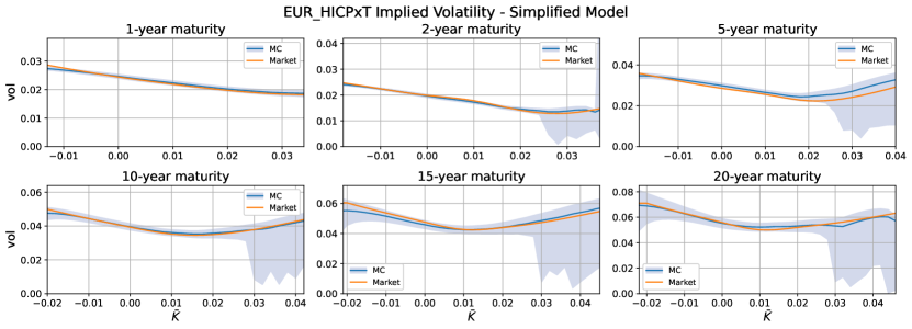
As in the previous subsection, we simulate the calibrated model over 2000 paths to price caps at various maturities and strikes. We compute the model implied volatilities from the Monte Carlo prices by inverting the pricing formula (4.8). Figure 4.4 shows that the market implied volatilities are within two Monte Carlo errors of the simulation means for most strikes within the test range. Moreover comparison to Figure 4.3 reveals that the simplified model performs similarly to the leveraged model in terms of accuracy.

Refer to caption
Figure 4.4: Market and Monte Carlo implied volatilities for the simplified model (4.25) with $M=3$ factors (4.3) for EUR inflation as of 2023-04-28. The market implied volatilities are within two Monte Carlo standard errors (blue shaded regions) for most strikes.

4.4 Pricing Example

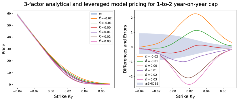
We simulate the leveraged model (4.12) and the simplified model (4.25) with 3 factors over 2000 paths to price 1-year to 2-year caps for several strikes with payoff defined in (3.8). We compare the Monte Carlo prices to the analytical prices given by (4.9). We note that the strike $K_{Y}$ of the year-on-year contract does not directly correspond to the strike $K$ that goes in $\Sigma_{i}(K)$ while calibrating the Kazziha parameter $\sigma_{i}$ to market volatilities by (4.7) for underlier $F_{i}$. If regular cap/floor quotes, e.g. $\Sigma_{i}(K)$, are only what is available as market data, one needs to pick a moneyness for the underlier $F_{i}$ to compute $\sigma_{i}$. Here we study the impact of this choice by computing analytical prices with $\bar{K}$ ranging from -0.02 to 0.03, where $K=F_{i}(0)(1+\bar{K})^{T_{i}}$.

Figure 4.5 compares the Monte Carlo prices for the leveraged model to the analytical prices computed by (4.9). Similarly, Figure 4.6 shows the comparison between the Monte Carlo prices for the simplified model to the analytical prices. The first observation is that both the leveraged and the simplified model give similar prices. The second observation is, the analytical model prices vary significantly by the choice of individual underlier moneynesses ($\bar{K}$) when calibrating the Kazziha parameter $\sigma_{i}$ to market volatilities $\Sigma_{i}(K)$. For both the leveraged and the simplified models, the simulated model prices are close to the analytical prices, that is the differences are within two standard errors for most strikes in the test range, only if we choose the individual underlier moneynesses close to at-the-money ($\bar{K}\rightarrow 0$) during the analytical price computation.

Refer to caption
Figure 4.5: Monte Carlo 1-year to 2-year cap prices for the leveraged model (4.12) with $M=3$ factors (4.3) for EUR inflation as of 2023-04-28 and notional $N=1000$, compared to analytical prices computed with several individual underlier moneynesses $\bar{K}$. The analytical prices are within two Monte Carlo standard errors (blue shaded regions) for most strikes when individual underlier moneynesses are chosen near at-the-money ($\bar{K}\rightarrow 0$).
Refer to caption
Figure 4.6: Monte Carlo 1-year to 2-year cap prices for the simplified model (4.25) with $M=3$ factors (4.3) for EUR inflation as of 2023-04-28 and notional $N=1000$, compared to analytical prices computed with several individual underlier moneynesses. The analytical prices are within two Monte Carlo standard errors (blue shaded regions) for most strikes when individual underlier moneynesses are chosen near at-the-money ($\bar{K}\rightarrow 0$).

5 Discussion

After reviewing the dynamics of the single-factor Kazziha inflation model coupled with single-factor G1++ interest rate model, we explored multi-factor inflation models that can be calibrated to historical correlations between inflation index underliers of available maturities. The multi-factor model (4.1) that we propose is analytically tractable, and we give closed form solutions for the prices of the inflation instruments under consideration. This model can be calibrated to regular or year-on-year caps/floors provided there is market data available. If year-on-year market data is unavailable, one can still calibrate individual underliers to available regular cap/floor market data. In this case, however, the individual underlier moneyness that one picks has an impact on the analytical year-on-year cap/floor price.

We further extended the multi-factor model with leverage functions (4.12) to capture the market skew nonparametrically. We proposed a slice-by-slice calibration methodology for the leverage functions using Monte Carlo simulation, and demonstrated that the calibrated model captures the market skew in volatility. By ignoring terms of small size in the expression of the leverage function, we formulated a simplified multi-factor model (4.25) which does not require the calibration step. Remarkably the simplified model replicates the market skew as well as the full leveraged model, and also produces similar year-on-year cap/floor prices. We compared the year-on-year cap prices of the leveraged and simplified models to the analytical prices with Kazziha parameter calibrated to several underlier moneynesses. We observed that the analytical prices are closer to leveraged or simplified model prices when the individual underlier moneynesses are chosen close to zero. The leveraged and simplified models do not have this ambiguity as they are constructed to capture the skew at all moneynesses, instead of a target moneyness.

Acknowledgments

The authors thank Agus Sudjianto for his support on research throughout the years leading into this work, and Vijayan Nair for his comments and suggestions regarding this work. Any opinions, findings and conclusions or recommendations expressed in this material are those of the authors and do not necessarily reflect the views of Wells Fargo Bank, N.A., its parent company, affiliates and subsidiaries.

References

  • [1] Marcin Wojtowicz. Inflation-linked bonds explained. Technical report, ETF & Index Fund Investment Analytics, UBS AM, 2023. ubs.com.
  • [2] Hringur Gretarsson. A Quadratic Gaussian Year-on-Year Inflation Model. PhD thesis, Imperial College London, 2013. spiral.imperial.ac.uk.
  • [3] Fabio Mercurio and Nicola Moreni. Inflation modelling with sabr dynamics. Risk, 22(6):98, 2009. SSRN:1337811.
  • [4] Robert A. Jarrow and Yildiray Yildirim. Pricing treasury inflation protected securities and related derivative securities using an hjm model. Journal of Financial and Quantitative Analysis, 38(2):337–58, 2003. SSRN:585828.
  • [5] Soraya Kazziha. Interest rate models, inflation-based derivatives, trigger notes and crosscurrency swaptions. PhD thesis, Imperial College of Science, Technology and Medicine, London, 1999.
  • [6] Nabyl Belgrade, Eric Benhamou, and Etienne Koehler. A market model for inflation. Cahiers de la maison des sciences economiques, Université Panthéon-Sorbonne (Paris 1), 2004. SSRN:576081.
  • [7] Fabio Mercurio. Pricing inflation-indexed derivatives. Quantitative Finance, 5(3):289–302, 2005. citeseerx.ist.psu.edu.
  • [8] Matthew J. W. Dodgson and Dherminder Kainth. Inflation-linked derivatives. Technical report, QuaRC, Group Market Risk, Royal Bank of Scotland Group, 2006. citeseerx.ist.psu.edu.
  • [9] Flavia Antonacci, Cristina Costantini, Fernanda D’Ippoliti, and Marco Papi. Risk neutral valuation of inflation-linked interest rate derivatives, 2019. arXiv:1911.00386.
  • [10] Fabio Mercurio and Nicola Moreni. Inflation with a smile. Risk, 19(3):70–75, 2006. risk.net.
  • [11] Vivien Begot. Stochastic local volatility models for inflation, 2016. lexifi.com.
  • [12] L.B.G. Andersen and V.V. Piterbarg. Interest Rate Modeling. Number v. 1 in Interest Rate Modeling. Atlantic Financial Press, 2010.
  • [13] Orcan Ögetbil, Narayan Ganesan, and Bernhard Hientzsch. Calibrating Local Volatility Models with Stochastic Drift and Diffusion. International Journal of Theoretical and Applied Finance, 25(02):2250011, 2022. arXiv:2009.14764.
  • [14] Leif Andersen. Markov models for commodity futures: Theory and practice. Quantitative Finance, 10(8):831–854, 2010. SSRN:1138782.
  • [15] Orcan Ögetbil and Bernhard Hientzsch. Extensions of Dupire Formula: Stochastic Interest Rates and Stochastic Local Volatility. SIAM Journal on Financial Mathematics, 14(2):452–474, 2023. arXiv:2005.05530.
  • [16] J. Gatheral. The Volatility Surface: A Practitioner’s Guide. Wiley finance series. John Wiley & Sons, 2006. wiley.com.
  • [17] Sébastien Gurrieri, Masaki Nakabayashi, and Tony Wong. Calibration methods of Hull-White model. Technical report, Risk Management Department, Mizuho Securities, Tokyo, 2009. SSRN:1514192.