Mass function of stellar black holes as revealed by the LIGO-Virgo-KAGRA observations
Abstract
Ninety gravitational wave events have been detected by the LIGO-Virgo-KAGRA network and are released in the Gravitational-Wave Transient Catalog. Among these events, 83 cases are definitely binary black hole mergers since the masses of all the objects involved significantly exceed the upper limit of neutron stars. The black holes in these merger events naturally form two interesting samples, a pre-merger sample that includes all the black holes before the mergers and a post-merger sample that consists of the black holes generated during the merging processes. The former represents black holes that once existed in the Universe, while the latter represents newly born black holes. Here we present a statistical analysis on these two samples. The non-parametric statistic method is adopted to correct for the observational selection effect. The Lynden-Bell’s method is further applied to derive the mass distribution and density function of black holes. It is found that the mass distribution can be expressed as a broken power-law function. More interestingly, the power-law index in the high mass region is comparable for the two samples. The number density of black holes is found to depend on redshift as – based on the two samples. Implications of these findings on the origin of black holes are discussed.
1 Introduction
As the first gravitational wave (GW) event being detected, GW150914 was produced by the merger of two black holes (BHs) whose masses are and , respectively (Abbott et al., 2016). Since then, the LIGO-Virgo-KAGRA (LVK) gravitational wave detector network (LIGO Scientific Collaboration et al., 2015; Acernese et al., 2015; Akutsu et al., 2018) has recorded about 90 confident binary merger events, which are reported in the Gravitational-Wave Transient Catalog (GWTC) 111https://gwosc.org/ (Abbott et al., 2021a, 2023a; The LIGO Scientific Collaboration et al., 2023). While the possibility that neutron stars might be involved in two or three GW events still cannot be completely expelled, it is believed that the majority of the GW events were produced by binary black hole (BBH) mergers. In fact, among the 90 GW events, at least 83 candidates come from BBH systems with the black hole mass ranging in 5 – 140 (Chattopadhyay et al., 2023; Abbott et al., 2023b). These GW events thus provide a valuable sample of stellar mass black holes.
GW observations provide useful information on the masses and distances of the black hole members, which can be used to probe the binary origin. There are many opinions on the origin of binary black holes, such as binaries in the field area of galaxies with a relatively low stellar density (Bethe & Brown, 1998; Giacobbo & Mapelli, 2018; Gallegos-Garcia et al., 2021; The LIGO Scientific Collaboration et al., 2023), dynamically-driven BBHs in dense stellar clusters (Portegies Zwart & McMillan, 2000; Banerjee et al., 2010; Rodriguez et al., 2016; Chattopadhyay et al., 2022), BBHs originated from triple systems (Antonini et al., 2017; Martinez et al., 2020; Vigna-Gómez et al., 2021) or via gas capture in the disks of active galactic nuclei (McKernan et al. (2012); Bartos et al. (2017); Fragione et al. (2019); Tagawa et al. (2020)). The exact processes that give birth to the BBHs detected by LVK have not yet been conclusively determined (Fakhry, 2024). The number of BHs existed in a unit comoving volume, i.e., the comoving BH number density, can provide information on the number of BHs formed at a certain redshift and can help to understand the progenitors of BHs at various stages of evolution (Lloyd-Ronning et al., 2002). However, there are several selection effects in the GW observations of BBHs, which prevent us from deriving the redshift distribution and mass distribution of BHs directly. As a result, the number densities of BHs in BBH systems could be derived only when the selection effects are properly accounted for.
The Lynden-Bell’s method (Lynden-Bell, 1971) is usually used to solve mutually independent truncated bivariate data distributions. It has been applied in many fields of astronomy, such as short/long gamma-ray bursts (Lloyd-Ronning et al., 2002; Yu et al., 2015; Pescalli et al., 2016; Zhang & Wang, 2018; Liu et al., 2021; Dong et al., 2022, 2023; Li et al., 2024), fast radio bursts (Deng et al., 2019), galaxies (Kirshner et al., 1978; Loh & Spillar, 1986; Peterson et al., 1986) and quasars (Singal et al., 2011; Zeng et al., 2021). The method is quite useful in deriving the intrinsic luminosity functions of various objects based on their flux and redshift measurements. Interestingly, it is also proved to be effective in correcting for the observational selection effects whenever a bivariate (or, more generally, multivariate) distribution is involved (Lynden-Bell, 1971; Efron & Petrosian, 1992, 1999; Dainotti et al., 2015; Levine et al., 2022).
A key assumption in the method is about the data independence. Therefore, it is important to ensure the independence of the truncated data. The statistic method is a unique non-parametric technique widely applied to truncated data for assessing the independence of parameters Efron & Petrosian (1992). The joint operation of the statistic method and Lynden-Bell’s method provides an ideal non-parametric method. It is extremely effective for a truncated sample since it does not depend on any pre-assumed models and can give a point-by-point description of the cumulative distribution.
In this study, we adopt the non-parametric method to explore the mass function and redshift distribution of BHs associated with BBH mergers. The BH number density will also be derived based on the analysis. The structure of our paper is organized as follows. In Section 2, data acquisition and the two BH samples used for the analysis are described. Section 3 introduces the non-parametric method and the calculation processes in detail. The numerical results are presented in Section 4. Finally, we end up with our conclusions and discussion in Section 5.
2 BBH merger events
The LVK gravitational wave detector network has completed three rounds of observation operations (O1/O2/O3) as of March 27, 2020 (Abbott et al., 2018). It began the fourth observing run on May 24, 2023. The online GWTC is a cumulative set of gravitational wave transients maintained by the LVK collaboration. It contains confirmed GW events from multiple data releases. Totally 90 GW events are included in the catalog as of March 27, 2020. Note that in 7 events, the mass of at least one binary member is not massive enough to be definitely identified as a black hole. In other words, these 7 events might be generated by binary neutron star mergers or neutron star-BH mergers. Since we are only interested in BBH mergers here, we exclude these GW events in our analyses.
Recently, the LVK collaboration specially reported a new GW event, GW230529_181500, detected during a preliminary analysis of the O4 data (The LIGO Scientific Collaboration et al., 2024). It seems to be produced by the coalescing of a less massive compact binary, with the masses of the two objects ranging in 2.5 – 4.5 and 1.2 – 2.0 . As a typical lower mass gap system, it is widely believed that the compact stars involved are neutron stars, although the possibility that they are BHs still cannot be excluded (Huang et al., 2024). Considering this uncertainty, we do not include the event in our study.
To sum up, we have 83 GW events in which all the compact objects are confirmed BHs. Our sample is composed of these BHs. For each GW event, we denote the mass of the heavier companion as and the mass of the lighter BH as . The mass of the final product of the merger, i.e. the newly born massive BH, is denoted as . Note that during the GW observation of a merger event, the unknown spin of each black hole will affect the estimated BH masses. In the GWTC catalog, the BH masses are estimated based on the assumption that the BH spins are in accordance with the angular speed of the innermost stable circular orbit. For a GW event, the chirp mass and mass ratio can be derived from the waveform information. The values of , and can then be determined from the chirp mass and (Poisson & Will, 1995; Hannam et al., 2013). To assess the event rate of BBH mergers, we need the redshift () information, which is also available in the GWTC catalog (Abbott et al., 2018). The relevant parameters of these BHs have been taken from the GWTC website and are listed in Table LABEL:tab:1 (Abbott et al., 2016, 2021a, 2023a).
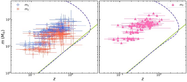
All the confirmed BHs are further divided into two samples. The first sample is called the pre-merger sample (), which includes all the separate black holes in the binary systems before the merging process. So, the number of BHs in the sample is . It represents one part of the confirmed BHs once existed in the universe. The second sample is called the post-merger sample (), which includes all the BHs produced after the merger. The number of BHs in the sample is simply 83. It represents the newly born BHs observed in the universe, which can also be regarded as a sample of stellar BHs at the relatively higher mass segment. Figure 1 plots the distribution of the two samples of BHs on the mass-redshift plane.
In our study, we assume a flat -CDM cosmology with the Hubble parameter and the density parameters taken as , , and . It is consistent with the cosmology parameters taken by the LVK collaboration (Planck Collaboration et al., 2016; Abbott et al., 2018, 2023a).
3 The non-parametric method
The mass function and number density of BHs can be inferred from the observed BH samples given that the BH masses and redshifts are available. However, note that the BH samples are truncated due to the detection threshold of the GW detectors. In Figure 1, the dashed line shows the truncation line, which represents the maximum redshift of BHs that the upgraded (A+) Advanced LIGO can detect when the signal-to-noise ratio is no less than 8 (Evans et al., 2021). The observational bias caused by this truncation line should be considered when we try to reconstruct the intrinsic distributions of BHs based on the observational data.
The BHs form a bivariate sample with two truncated parameters, i.e. mass () and redshift (). The joint distribution of BHs is a function of both mass and distance, which can be written as . If the dependence of the joint distribution on the two parameters is independent of each other, then we have , where represents the mass function and represents the redshift distribution of black holes. The Lynden-Bell’s method (Lynden-Bell, 1971) is suitable for dealing with such mutually independent bivariate problems, which can help obtain the number density of the black holes. Therefore, ensuring the independence of the bivariate truncated data is the basis for us to get a meaningful statistical results from the BBH mass and redshift observations (Efron & Petrosian, 1992, 1999).
In Figure 1, there is a clear positive correlation between the observed mass and redshift for both the pre-merger sample and the post-merger sample. This may be caused by the observational selection effect (Hirai & Mandel, 2021; Okano & Suyama, 2023; Karathanasis et al., 2023). A GW detector has a limited sensitivity. It can sensitively record nearby GW events. But for distant mergers, it can only detect those events involving relatively massive BHs. Such an observational selection effect also needs to be corrected for before drawing firm conclusions on the intrinsic distribution of BHs. Therefore, in this section, we first introduce the method to remove the dependence between mass and redshift and then describe how to apply the Lynden-Bell’s method to bivariate independent parameter samples to obtain the BH mass function, redshift distribution and number density.
3.1 The method of statistics
The non-parametric statistic method (Efron & Petrosian, 1992, 1999) can be applied to remove the bias caused by observational selection effects, i.e. the induced correlation between and . When this method is used in other fields such as gamma-ray bursts and fast radio bursts, it is usually assumed that a power-law relation exists between the luminosity and the redshift due to the observational selection effects (Conselice et al., 2020; Babak et al., 2023). Similarly, in this study, we use to represent the biased dependence of mass on the redshift, where is a constant. Once the power-law index is determined, we then can correct the mass as . In this way, we can get the independent parameter pair of and , which means the BH distribution function can be expressed as .
The value of could be determined from the observational data. For a specific , the observed data point of each black hole will change from to the corrected point of . For the th data point in the BH sample, we first define a data set as
| (1) |
where is the corrected mass of the th BH and is the maximum redshift at which a BH with mass can be detected by the detector. The number of BHs contained in this region is denoted as , and the number of BHs with redshift less than or equal to in this region is designated as . The test statistic is expressed as
| (2) |
where and are the expected mean value and the variance of , respectively.
According to the statistic test, if is uniformly distributed between 1 and , then the probability of and should be nearly equal so that we have . In this case, we could know that the distribution of mass and redshift are independent of each other. It means that the assumed value can correctly remove the bias introduced by the observational selection effect. On the other hand, if does not equal zero, then we need to adjust the value of . The above calculation process is repeated until is satisfied and the correct value is determined.
During the calculations, the truncation line is a key ingredient which is used to calculate . However, note that the truncation line in Figure 1 is a complex function which could not be described by a simple analytical equation. Luckily, for our BH samples, the limit curve in the region does not have any impact on the statistics of the non-parametric method. Consequently, we are only concerned about the limit curve in the segment. In this region, we notice that the limit curve in fact could be well represented by a simple straight line of (i.e. the solid line in the figure). So, we use this straight line as the the effective truncation limit to perform our calculations.
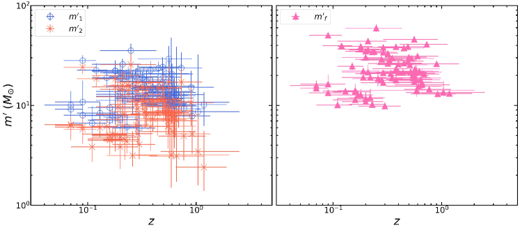
Using this method of statistics, we finally get the best value as for the pre-merger sample and for the post-merger sample. The observed BH masses are then corrected by dividing them with . The distributions of the BHs after correction are shown in Figure 2. It can be seen that the masses of the black holes no longer show any correlation with the redshifts.
3.2 The Lynden-Bell’s method
The Lynden-Bell’s method is an effective way to derive the bivariate distributions of astronomical objects from the truncated data. In Equation (1), the number of BHs in the region of is . The Lynden-Bell’s method does not include the th BH in the analysis, which means the BH number is smaller by 1, i.e. . This is the reason that the method is called the “” method (Lynden-Bell, 1971). To carry out the calculations, we need to further define another set as
| (3) |
where is the limit mass at the redshift . We denote the number of BHs in as .
According to the Lynden-Bell’s method, the cumulative mass function can then be calculated as (Lynden-Bell, 1971; Efron & Petrosian, 1992)
| (4) |
where means that the operation applies to all BHs whose mass is larger than . Similarly, the cumulative redshift distribution can be expressed as
| (5) |
where means that the operation applies to all BHs whose redshift is less than .
The number density of BHs can be written as
| (6) |
where the term of results from the cosmological time dilation and is the differential comoving volume which can be further expressed as (Khokhriakova & Popov, 2019)
| (7) |
Note that the comoving volume at a redshift of is , where the comoving distance is (Hogg 1999).
4 results
We have applied the unbiased non-parametric statistics method on the pre-merger and post-merger BH samples to correct for the dependence between mass and redshift of BHs induced by the observational selection effects. The Lynden-Bell’s method is then used to derive the intrinsic mass function and redshift distribution of BHs based on the two samples. Additionally, the number density of BHs in the Universe is inferred by considering the redshift information of the BHs. Here we present our numerical results as follows.
4.1 Mass distribution function
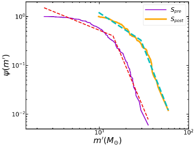
The mass distribution function of BHs can be calculated by using Equation (4). The results derived from the pre-merger sample and the post-merger sample are shown in Figure 3. We see that for both samples, the mass function shows a decreasing trend with the increasing mass. However, it is obvious that the mass distribution of the pre-merger sample is different from that of the post-merger sample. In the former case, the mass is mainly distributed between 2 and 40 ; while it is in a range of 10 – 60 in the latter case. It clearly shows that the post-merger BHs are significantly more massive.
We have used a simple broken power law function to fit the mass distribution function, i.e.
| (8) |
where is the mass at the broken position, and are the two power-law indices characterizing the steepness of the mass function before and after the broken. The best fitting results of the pre-merger sample are , , and . For the post-merger sample, the best fitting results are , , and . The results are shown by the dashed lines in Figure 3. We see that the broken mass of of the post-merger sample is significantly larger than that of the pre-merger sample. This is easy to understand since the BHs in the post-merger sample are generally more massive. It is interesting to note that the power-law index in the high mass segment, i.e. , is generally consistent with each other for the two samples, which means that the mass function of BHs has a steep index of – . On the other hand, the index of is clearly different for the two samples. The reason may be that there are too few less massive BHs in the post-merger sample.
4.2 Redshift distribution and number density of BHs
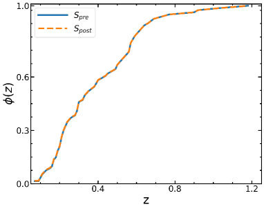
The cumulative redshift distribution of the two BH samples can be calculated by using Equation (5). The results are shown in Figure 4. We see that the cumulative distribution is almost identical for the two samples. This is easy to understand, since each post-merger BH corresponds to two pre-merger BHs at a particular redshift. Also, it is interesting to note that the cumulative distribution increases rapidly at two redshifts, i.e. and . It indicates that there are more BHs at these two distances.
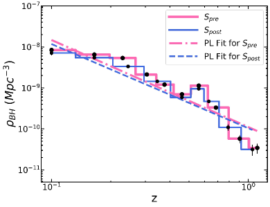
After obtaining the redshift distribution, we have further calculated the number density of black holes by using Equation (6). The number density is plot versus redshift in Figure 5 for the two BH samples. We see that for both BH samples, the number density decreases steadily as the redshift increases. The behavior can be well fited by a power-law function in the form of , where is the power-law index. For the pre-merger sample, the best-fit value is . For the post-merger sample, we have . Interestingly, these two indices are consistent with each other, suggesting that the number density of BHs in the two samples has a similar redshift dependence. Furthermore, from Figure 5, we can notice that the number density has a slight excess at 0.2 – 0.3 and 0.5 – 0.6, which is exactly the reason that leads to the two rapidly increasing episodes illustrated in Figure 4.
5 Conclusions and Discussion
Ninety credible GW events are released in the GWTC catalogue by the LVK collaboration, among which 83 cases are confirmed binary black hole mergers. In this study, we have carried out a statistical analysis on the masses and redshifts of these BHs. Two samples consisted of the 166 pre-merger BHs and the 83 post-merger BHs are considered separately, with the former sample representing BHs that once exist in the Universe and the latter representing newly born BHs. The non-parametric statistic method is adopted to remove the bias caused by observational selection effect, which leads to a dependence between redshift and mass as for the pre-merger sample and for the post-merger sample. After correcting for the selection effect, the mass and redshift become two independent parameters for the two samples, based on which meaningful statistical analysis can be carried out. Using the Lynden-Bell’s method, it is found that the mass distribution can be expressed as a broken power-law function for both samples. In the case of the pre-merger sample, the power-law indices are and in the smaller mass region and the higher mass region, respectively, with the break occurring at . For the post-merger sample, the indices are and correspondingly, with the broken mass being . We notice that the power-law index in the higher mass region is essentially identical for the two samples. Additionally, the number density of BHs is derived as – from the two samples.
The merger rate of binary black hole systems has been explored by many groups (Spera et al., 2019; Antonini & Gieles, 2020; Abbott et al., 2021b; He et al., 2023; Fishbach & Fragione, 2023; Cui & Li, 2023; Fakhry, 2024), with different conclusions being reached. For example, Conselice et al. (2020) studied the merger process of black holes in ultra low-mass dwarf galaxies. Although their merger rate is high enough to account for the gravitational wave events detected by LIGO/Virgo, a special feature of their results is that the rate increases with the increasing redshift under various time delay assumptions. On the other hand, Vijaykumar et al. (2023) argued that if BBHs were hosted by a sample of galaxies purely weighted by their stellar mass, then the BBH number density would roughly decrease with the increasing redshift as . The different outcomes on BBH rates may result from different assumptions and different samples being used. It also reflects the complexity of this difficult problem. In our study, we have used a non-parametric method in which as fewer assumptions are made as possible. Additionally, our study is based on the unified GW events detected by the LVK collaboration. So, it is a beneficial attempt on this issue.
It deserves mentioning that the BHs in our post-merger samples are universally produced via the merging of two smaller BHs. However, the origin of the BHs in the pre-merger sample is uncertain. Theoretically, they could come from direct collapse of old massive stars, growth of less massive BHs through accretion, or merging of two BHs. The similarity of some features between the two samples, such as the consistent power-law index of the mass distribution function in the higher mass region, and the almost equal power-law index of the number density, could potentially provide interesting information on the origin of the pre-merger BHs. It points to the possibility that the majority of them, especially those at the higher mass end, should also be of merger origin. Currently, the number of BHs in the two samples is still very limited. The fourth observing run (O4) of LVK is still in progress. When it ends in February 2025, the total number of detected GW events is expected to exceed 200. A much larger catalogue of BBHs will be available, which will be helpful for us to further explore the origin and distribution of BHs in the Universe.
6 Acknowledgements
We are grateful to Yi-Han Iris Yin for helpful discussions. This study was supported by the National Natural Science Foundation of China (Grant Nos. 12233002, U2031118), by the National SKA Program of China No. 2020SKA0120300, by the National Key R&D Program of China (2021YFA0718500). LXJ acknowledges the support by Shandong Provincial Natural Science Foundation (Grant No. ZR2023MA049). YFH also acknowledges the support from the Xinjiang Tianchi Program.
References
- Abbott et al. (2016) Abbott, B. P., Abbott, R., Abbott, T. D., et al. 2016, Phys. Rev. Lett., 116, 061102, doi: 10.1103/PhysRevLett.116.061102
- Abbott et al. (2018) —. 2018, Living Reviews in Relativity, 21, 3, doi: 10.1007/s41114-018-0012-9
- Abbott et al. (2021a) Abbott, R., Abbott, T. D., Abraham, S., et al. 2021a, Physical Review X, 11, 021053, doi: 10.1103/PhysRevX.11.021053
- Abbott et al. (2021b) —. 2021b, ApJ, 913, L7, doi: 10.3847/2041-8213/abe949
- Abbott et al. (2023a) Abbott, R., Abbott, T. D., Acernese, F., et al. 2023a, Physical Review X, 13, 041039, doi: 10.1103/PhysRevX.13.041039
- Abbott et al. (2023b) —. 2023b, Physical Review X, 13, 011048, doi: 10.1103/PhysRevX.13.011048
- Acernese et al. (2015) Acernese, F., Agathos, M., Agatsuma, K., et al. 2015, Classical and Quantum Gravity, 32, 024001, doi: 10.1088/0264-9381/32/2/024001
- Akutsu et al. (2018) Akutsu, T., Ando, M., Araki, S., et al. 2018, Progress of Theoretical and Experimental Physics, 2018, 013F01, doi: 10.1093/ptep/ptx180
- Antonini & Gieles (2020) Antonini, F., & Gieles, M. 2020, Phys. Rev. D, 102, 123016, doi: 10.1103/PhysRevD.102.123016
- Antonini et al. (2017) Antonini, F., Toonen, S., & Hamers, A. S. 2017, ApJ, 841, 77, doi: 10.3847/1538-4357/aa6f5e
- Babak et al. (2023) Babak, S., Caprini, C., Figueroa, D. G., et al. 2023, J. Cosmology Astropart. Phys, 2023, 034, doi: 10.1088/1475-7516/2023/08/034
- Banerjee et al. (2010) Banerjee, S., Baumgardt, H., & Kroupa, P. 2010, MNRAS, 402, 371, doi: 10.1111/j.1365-2966.2009.15880.x
- Bartos et al. (2017) Bartos, I., Kocsis, B., Haiman, Z., & Márka, S. 2017, ApJ, 835, 165, doi: 10.3847/1538-4357/835/2/165
- Bethe & Brown (1998) Bethe, H. A., & Brown, G. E. 1998, ApJ, 506, 780, doi: 10.1086/306265
- Chattopadhyay et al. (2022) Chattopadhyay, D., Hurley, J., Stevenson, S., & Raidani, A. 2022, MNRAS, 513, 4527, doi: 10.1093/mnras/stac1163
- Chattopadhyay et al. (2023) Chattopadhyay, D., Stegmann, J., Antonini, F., Barber, J., & Romero-Shaw, I. M. 2023, MNRAS, 526, 4908, doi: 10.1093/mnras/stad3048
- Conselice et al. (2020) Conselice, C. J., Bhatawdekar, R., Palmese, A., & Hartley, W. G. 2020, ApJ, 890, 8, doi: 10.3847/1538-4357/ab5dad
- Cui & Li (2023) Cui, Z., & Li, X.-D. 2023, MNRAS, 523, 5565, doi: 10.1093/mnras/stad1800
- Dainotti et al. (2015) Dainotti, M., Petrosian, V., Willingale, R., et al. 2015, MNRAS, 451, 3898, doi: 10.1093/mnras/stv1229
- Deng et al. (2019) Deng, C.-M., Wei, J.-J., & Wu, X.-F. 2019, Journal of High Energy Astrophysics, 23, 1, doi: 10.1016/j.jheap.2019.05.001
- Dong et al. (2022) Dong, X. F., Li, X. J., Zhang, Z. B., & Zhang, X. L. 2022, MNRAS, 513, 1078, doi: 10.1093/mnras/stac949
- Dong et al. (2023) Dong, X. F., Zhang, Z. B., Li, Q. M., Huang, Y. F., & Bian, K. 2023, ApJ, 958, 37, doi: 10.3847/1538-4357/acf852
- Efron & Petrosian (1992) Efron, B., & Petrosian, V. 1992, ApJ, 399, 345, doi: 10.1086/171931
- Efron & Petrosian (1999) —. 1999, Journal of the American Statistical Association, 94, 824
- Evans et al. (2021) Evans, M., Adhikari, R. X., Afle, C., et al. 2021, arXiv e-prints, arXiv:2109.09882, doi: 10.48550/arXiv.2109.09882
- Fakhry (2024) Fakhry, S. 2024, ApJ, 961, 8, doi: 10.3847/1538-4357/ad0e66
- Fishbach & Fragione (2023) Fishbach, M., & Fragione, G. 2023, MNRAS, 522, 5546, doi: 10.1093/mnras/stad1364
- Fragione et al. (2019) Fragione, G., Leigh, N. W. C., & Perna, R. 2019, MNRAS, 488, 2825, doi: 10.1093/mnras/stz1803
- Gallegos-Garcia et al. (2021) Gallegos-Garcia, M., Berry, C. P. L., Marchant, P., & Kalogera, V. 2021, ApJ, 922, 110, doi: 10.3847/1538-4357/ac2610
- Giacobbo & Mapelli (2018) Giacobbo, N., & Mapelli, M. 2018, MNRAS, 480, 2011, doi: 10.1093/mnras/sty1999
- Hannam et al. (2013) Hannam, M., Brown, D. A., Fairhurst, S., Fryer, C. L., & Harry, I. W. 2013, ApJ, 766, L14, doi: 10.1088/2041-8205/766/1/L14
- He et al. (2023) He, J.-G., Shao, Y., Gao, S.-J., & Li, X.-D. 2023, ApJ, 953, 153, doi: 10.3847/1538-4357/ace348
- Hirai & Mandel (2021) Hirai, R., & Mandel, I. 2021, PASA, 38, e056, doi: 10.1017/pasa.2021.53
- Hogg (1999) Hogg, D. W. 1999, arXiv e-prints, astro, doi: 10.48550/arXiv.astro-ph/9905116
- Huang et al. (2024) Huang, Q.-G., Yuan, C., Chen, Z.-C., & Liu, L. 2024, arXiv e-prints, arXiv:2404.05691, doi: 10.48550/arXiv.2404.05691
- Karathanasis et al. (2023) Karathanasis, C., Mukherjee, S., & Mastrogiovanni, S. 2023, MNRAS, 523, 4539, doi: 10.1093/mnras/stad1373
- Khokhriakova & Popov (2019) Khokhriakova, A. D., & Popov, S. B. 2019, Journal of High Energy Astrophysics, 24, 1, doi: 10.1016/j.jheap.2019.09.004
- Kirshner et al. (1978) Kirshner, R. P., Oemler, A., J., & Schechter, P. L. 1978, AJ, 83, 1549, doi: 10.1086/112363
- Levine et al. (2022) Levine, D., Dainotti, M., Zvonarek, K. J., et al. 2022, ApJ, 925, 15, doi: 10.3847/1538-4357/ac4221
- Li et al. (2024) Li, Q. M., Sun, Q. B., Zhang, Z. B., Zhang, K. J., & Long, G. 2024, MNRAS, 527, 7111, doi: 10.1093/mnras/stad3619
- LIGO Scientific Collaboration et al. (2015) LIGO Scientific Collaboration, Aasi, J., Abbott, B. P., et al. 2015, Classical and Quantum Gravity, 32, 074001, doi: 10.1088/0264-9381/32/7/074001
- Liu et al. (2021) Liu, Z.-Y., Zhang, F.-W., & Zhu, S.-Y. 2021, Research in Astronomy and Astrophysics, 21, 254, doi: 10.1088/1674-4527/21/10/254
- Lloyd-Ronning et al. (2002) Lloyd-Ronning, N. M., Fryer, C. L., & Ramirez-Ruiz, E. 2002, ApJ, 574, 554, doi: 10.1086/341059
- Loh & Spillar (1986) Loh, E. D., & Spillar, E. J. 1986, ApJ, 307, L1, doi: 10.1086/184717
- Lynden-Bell (1971) Lynden-Bell, D. 1971, MNRAS, 155, 95, doi: 10.1093/mnras/155.1.95
- Martinez et al. (2020) Martinez, M. A. S., Fragione, G., Kremer, K., et al. 2020, ApJ, 903, 67, doi: 10.3847/1538-4357/abba25
- McKernan et al. (2012) McKernan, B., Ford, K. E. S., Lyra, W., & Perets, H. B. 2012, MNRAS, 425, 460, doi: 10.1111/j.1365-2966.2012.21486.x
- Okano & Suyama (2023) Okano, S., & Suyama, T. 2023, Astrophys. Space Sci., 368, 5, doi: 10.1007/s10509-022-04160-4
- Pescalli et al. (2016) Pescalli, A., Ghirlanda, G., Salvaterra, R., et al. 2016, A&A, 587, A40, doi: 10.1051/0004-6361/201526760
- Peterson et al. (1986) Peterson, B. A., Ellis, R. S., Efstathiou, G., et al. 1986, MNRAS, 221, 233, doi: 10.1093/mnras/221.2.233
- Planck Collaboration et al. (2016) Planck Collaboration, Ade, P. A. R., Aghanim, N., et al. 2016, A&A, 594, A13, doi: 10.1051/0004-6361/201525830
- Poisson & Will (1995) Poisson, E., & Will, C. M. 1995, Phys. Rev. D, 52, 848, doi: 10.1103/PhysRevD.52.848
- Portegies Zwart & McMillan (2000) Portegies Zwart, S. F., & McMillan, S. L. W. 2000, ApJ, 528, L17, doi: 10.1086/312422
- Rodriguez et al. (2016) Rodriguez, C. L., Chatterjee, S., & Rasio, F. A. 2016, Phys. Rev. D, 93, 084029, doi: 10.1103/PhysRevD.93.084029
- Singal et al. (2011) Singal, J., Petrosian, V., Lawrence, A., & Stawarz, Ł. 2011, ApJ, 743, 104, doi: 10.1088/0004-637X/743/2/104
- Spera et al. (2019) Spera, M., Mapelli, M., Giacobbo, N., et al. 2019, MNRAS, 485, 889, doi: 10.1093/mnras/stz359
- Tagawa et al. (2020) Tagawa, H., Haiman, Z., Bartos, I., & Kocsis, B. 2020, ApJ, 899, 26, doi: 10.3847/1538-4357/aba2cc
- The LIGO Scientific Collaboration et al. (2024) The LIGO Scientific Collaboration, the Virgo Collaboration, & the KAGRA Collaboration. 2024, arXiv e-prints, arXiv:2404.04248, doi: 10.48550/arXiv.2404.04248
- The LIGO Scientific Collaboration et al. (2023) The LIGO Scientific Collaboration, the Virgo Collaboration, the KAGRA Collaboration, et al. 2023, arXiv e-prints, arXiv:2308.03822, doi: 10.48550/arXiv.2308.03822
- Vigna-Gómez et al. (2021) Vigna-Gómez, A., Toonen, S., Ramirez-Ruiz, E., et al. 2021, ApJ, 907, L19, doi: 10.3847/2041-8213/abd5b7
- Vijaykumar et al. (2023) Vijaykumar, A., Fishbach, M., Adhikari, S., & Holz, D. E. 2023, arXiv e-prints, arXiv:2312.03316, doi: 10.48550/arXiv.2312.03316
- Yu et al. (2015) Yu, H., Wang, F. Y., Dai, Z. G., & Cheng, K. S. 2015, ApJS, 218, 13, doi: 10.1088/0067-0049/218/1/13
- Zeng et al. (2021) Zeng, H., Petrosian, V., & Yi, T. 2021, ApJ, 913, 120, doi: 10.3847/1538-4357/abf65e
- Zhang & Wang (2018) Zhang, G. Q., & Wang, F. Y. 2018, ApJ, 852, 1, doi: 10.3847/1538-4357/aa9ce5
| () | () | () | |
|---|---|---|---|
Note. The data are taken from GWTC (https://gwosc.org/).