Longitudinal spin polarization in a thermal model with dissipative corrections
Abstract
In this work, we address the problem of longitudinal spin polarization of the hyperons produced in relativistic heavy-ion collisions. We combine a relativistic kinetic-theory framework that includes spin degrees of freedom treated in a classical way with the freeze-out parametrization used in previous investigations. The use of the kinetic theory allows us to incorporate dissipative corrections (due to the thermal shear and gradients of thermal vorticity) into the Pauli-Lubanski vector that determines spin polarization and can be directly compared with the experimental data. As in earlier similar studies, it turns out that a successful description of data can only be achieved with additional assumptions – in our case, they involve the use of projected thermal vorticity and a suitably adjusted time for spin relaxation (). From our analysis, we find that fm/, which is comparable with other estimates.
keywords:
spin polarization , kinetic theory , spin relaxation time , thermal models[a]organization=School of Physical Sciences, National Institute of Science Education and Research, An OCC of Homi Bhabha National Institute, city=Jatni, postcode=752050, country=India
[b]organization=Institute of Theoretical Physics, Jagiellonian University,city=Kraków, postcode=30-348, country=Poland
[c]organization=Institute of Nuclear Physics, Polish Academy of Sciences,city=Kraków, postcode=31-342, country=Poland
1 Introduction
One of the recent motivations for studying non-central heavy-ion collisions is to study the spin polarization effects of various produced particles, for example, hyperons [1, 2, 3] and vector mesons [4], for a recent review see Ref. [5] and for various related theoretical developments see Refs. [6, 7, 8, 9, 10, 11, 12, 13, 14, 15, 16, 17, 18, 19, 20, 21, 22, 23, 24, 25, 26, 27, 28, 29, 30, 31, 32, 33, 34, 35, 36]. In particular, there is a lot of interest in the measurement of the longitudinal spin polarization of ’s produced in Au-Au collisions at the beam energy of GeV [3]. In this case, the data indicates a quadrupole structure of the longitudinal polarization in the transverse momentum plane, which disagrees in sign with most theoretical predictions (the so-called sign problem) [37].
In this paper, we continue some of the earlier studies of the longitudinal polarization [38, 39] that use thermal model to parametrize freeze-out conditions in Au-Au collisions. A novel feature of the current analysis is that we incorporate dissipative corrections to the Pauli-Lubanski vector. They are determined within the framework of kinetic theory, which treats spin degrees of freedom classically [40]. This approach turns out to be consistent with the formalism that uses Wigner functions in the semiclassical expansion and considers GLW versions of the energy-momentum and spin tensors.
The most common approach in the polarization studies is to assume that the spin polarization tensor is given by the thermal vorticity
| (1) |
Here is the ratio of the hydrodynamic flow and temperature, . This leads to the expression for the Pauli-Lubanski vector that includes the spin equilibrium distribution function depending on . The kinetic-theory approach allows for including corrections to the equilibrium distributions. In our case, they are obtained from the kinetic equation treated in the relaxation time approximation (RTA) [41, 20, 42]. In this way, we naturally obtain contributions from the thermal shear
| (2) |
and gradients of thermal vorticity. We note that the effects due to the thermal shear were first considered in Refs. [43, 44, 45]. Thus, our approach offers yet another method to incorporate such corrections.
We use the freeze-out parametrization introduced in Ref. [46]. It turned out to be very successful in describing many observables like the transverse-momentum spectra or elliptic flow coefficients of various hadronic species. However, as the model is boost-invariant, it cannot reproduce the global spin polarization that points in the out-of-plane direction. On the other hand, as it correctly reproduces the elliptic flow, it is natural to use it in the studies of longitudinal polarization as these two phenomena are considered to be interconnected [5].
It has been demonstrated before that inclusion of the thermal shear helps to overcome the sign problem [43, 44, 45]. However, further conjectures were usually made to reproduce the data (for example, neglecting temperature gradients at freeze-out [45] or exchanging the mass by the strange quark mass [43]). In our case, we also introduce an additional assumption – it involves the use of projected thermal vorticity. By projected vorticity we mean the thermal vorticity tensor with all “electric” like components neglected, i.e., with . As found in our previous work [38], this procedure is consistent with a non-relativistic treatment where polarization is determined solely by the spatial components of the rotation [47].
The use of the projected thermal vorticity leads to a correct sign of the quadrupole structure of the longitudinal spin polarization, however, there remains a quantitative difference between theoretical predictions and the data [17]. In this work, we show that this disagreement can be removed by the inclusion of dissipative corrections described above with a suitably fitted spin relaxation time. Our numerical calculations show that a very good description of the effect can be obtained with the spin relaxation time fm/, which is in agreement with earlier estimates of the spin relaxation time [48, 49, 50, 51].
Notation and conventions: For the Levi-Civita tensor we follow the convention . The metric tensor is of the form . Throughout the text we make use of natural units, .
2 Spin observables at freeze-out
The mean spin polarization of hyperons can be found from the Pauli-Lubanski (PL) vector [12, 40]
| (3) |
where is the four-momentum with the on-mass-shell energy , is the mass ( GeV), is an infinitesimal element of the freeze-out hypersurface, and is the spin tensor discussed in more detail in A. Integration of Eq. (3) over the freeze-out hypersurface gives the momentum density of the PL vector
| (4) |
Here is defined as the ratio of the baryon chemical potential and temperature, is the spin polarization tensor, is the spin relaxation time, and .
As we are interested in the spin polarization per particle, we introduce the particle number density
| (5) |
A quantity which can be directly compared with the experimental results is the ratio of the integrated densities
| (6) |
Given the above theoretical setup, we use thermal vorticity as a proxy for the spin polarization tensor () and use it in the thermal model discussed in more detail below.
3 Thermal model
3.1 Freeze-out parametrization
In this work, we use a thermal model that assumes simultaneous kinetic and chemical freeze-outs [52, 53]. In its standard formulation, the single freeze-out model has only four parameters: temperature (), baryon chemical potential (), proper time (), and system size (). Temperature and chemical potential are inferred from the measured ratios of hadronic abundances, while the proper time and system size are extracted from the fits to the experimental transverse-momentum spectra. As we study collisions at ultrarelativistic energies we can set ().
As the effects of the longitudinal polarization are related to the phenomenon of elliptic flow, we adopt here an extended version of the single-freeze-out model [46] that allows for asymmetry of the hydrodynamic flow in the transverse plane
| (7) |
This introduces an additional parameter . For , the flow in the reaction plane(along -axis) is stronger than in the out-of-plane direction(along -axis), leading to the positive elliptic flow coefficients . The parameter is determined from the normalization condition , which gives
| (8) |
where is the proper time at freeze-out
| (9) |
Along with the asymmetric flow profile, we introduce the asymmetry of the fireball boundary in the transverse plane. This is achieved with the boundary parametrization of the form
| (10) |
where is the azimuthal angle. The parameter controls the spatial elongation of the system. For , the emitting source is elongated in the out-of-plane direction [54].
| cent. (%) | [fm] | [fm] | ||
|---|---|---|---|---|
| 0–15 | 0.055 | 0.12 | 7.666 | 6.540 |
| 15–30 | 0.097 | 0.26 | 6.258 | 5.417 |
| 30–60 | 0.137 | 0.37 | 4.266 | 3.779 |
Following earlier studies, we assume that freeze-out occurs at a fixed value of the proper time and temperature, denoted as and . Under these conditions, a three-dimensional component of the freeze-out hypersurface, denoted as , is expressed by the formula
| (11) |
where
| (12) |
satisfies the normalization condition and is the spacetime rapidity. The particle four-momentum can be parametrized in terms of the rapidity , transverse momentum , and the azimuthal angle as
| (13) |
with being the transverse mass.
3.2 Spin polarization at freeze-out
The thermal vorticity can be written as a sum of two terms
| (14) |
Similarly, we use the following decomposition for the thermal shear
| (15) |
The derivatives of the temperature can be determined from the hydrodynamic equations
| (16) |
where . We find that turns out to be the same as . The explicit expressions for all tensor components of can be found in Ref. [38]. The forms of and can be found in Ref. [39]. In this work, we consider [55], which affects the polarization results through Eq. (15). The derivatives of thermal vorticity () are listed in B.
4 Results and Discussion
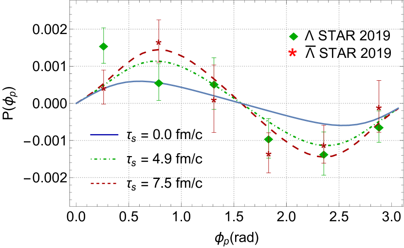
In this section, we present our numerical results for the -integrated longitudinal component of the mean Pauli-Lubanski four-vector, which characterizes the longitudinal spin polarization of the and hyperons. The model parameters utilized in the calculations are provided in Table 1. These parameters were previously fitted to describe the PHENIX data at the beam energy of GeV for three centrality classes: –, –, and –, at freeze-out temperature GeV.
As our primary interest lies in the longitudinal polarization, there is no need to boost the quantity back to the particle’s rest frame due to its invariance under transverse boosts. Additionally, to align with experimental practices, we solely focus on the central rapidity region (). We perform the transverse momentum () integral in the range from 0 to 3 GeV, and we have verified that extending the range to the experimental momentum range of 0.5–6.0 GeV does not significantly alter the results.

The magnitude of dissipative corrections depends on the value of the spin relaxation time . We observe that the inclusion of dissipative correction leads to an increase in the magnitude of longitudinal polarization. This feature may be attributed to the fact that dissipation results in increased conversion of fluid angular momentum to spin polarization. To determine the value of , we have performed a reduced chi-squared test. We find that the optimal description of the data for hyperons is achieved with fm/, corresponding to the reduced chi-squared value . On the other hand, for hyperons, we find good agreement with fm/ corresponding to . These values of the spin relaxation times are in agreement with those obtained in Refs. [48, 49, 50, 51].
In Fig. 1 we show the longitudinal polarization as a function of the azimuthal angle for 30–60% Au-Au collisions at GeV. Experimental data points are taken from [3], and conversion from to polarization helicity (PH) is conducted using [56]. Error bars represent the combined statistical and systematic uncertainties. The solid line represents our theoretical result without dissipative corrections, the dashed line corresponds to the dissipative case with , while the dashed-dotted line corresponds to . In Fig. 2 we present our theoretical predictions for two other centrality classes for the same colliding system.
5 Summary and conclusions
In this study, we addressed the issue of longitudinal spin polarization of hyperons generated in relativistic heavy-ion collisions. We employed a relativistic kinetic-theory framework, incorporating classical treatment of spin degrees of freedom, combined with the freeze-out parametrization utilized in prior investigations. By employing kinetic theory, we were able to include dissipative corrections, such as those arising from thermal shear and gradients of thermal vorticity, into the Pauli-Lubanski vector, which determines spin polarization. This allowed for direct comparison with experimental data. Similar to previous studies, we found that a comprehensive explanation of the data necessitated additional assumptions. Specifically, we employed projected thermal vorticity as a proxy to spin polarization tensor. The spin relaxation time was fitted to match the experimental data through a reduced chi-squared minimization procedure. The estimated spin relaxation time was found to be approximately fm/, which is consistent with earlier estimates [48, 49, 50, 51]. From this analysis, we conclude that dissipative corrections to spin tensor play an important role in explaining the observed longitudinal polarization in heavy-ion collisions.
Acknowledgements
The authors would like to thank Sourav Dey for useful discussions. S. Banerjee acknowledges the kind hospitality of Jagiellonian University, where part of this work was carried out. This work was supported in part by the Polish National Science Centre Grants No. 2022/47/B/ST2/01372 (W.F. and S. Banerjee) and No. 2018/30/E/ST2/00432 (R.R.).
Appendix A Pauli-Lubanski vector with dissipative corrections
In this section, we outline the steps to evaluate Eq. (4) starting from the kinetic theory expression of the non-equilibrium correction to phase-space distribution function, given by,
| (17) |
Using this we can determine the off-equilibrium correction to spin tensor as,
| (18) |
where we have used the result as derived in Refs. [40, 20] and the integral measures are defined as,
| (19) | ||||
| (20) |
Furthermore, using the relations [57, 40, 20],
| (21) | ||||
| (22) |
we can carry out the integration over spin to obtain,
| (23) |
where the square brackets imply anti-symmetric combination i.e., . The Pauli-Lubanski vector in Eq. (3) can then be expressed as
| (24) |
Integrating over the spacetime volume we can write,
| (25) |
with,
| (26) |
Appendix B Derivative of Thermal Vorticity Components
Here we list the derivatives of the “magnetic like” components of the thermal vorticity.
| (27) | ||||
| (28) | ||||
| (29) | ||||
| (30) | ||||
| (31) | ||||
| (32) | ||||
| (33) | ||||
| (34) | ||||
| (35) | ||||
| (36) | ||||
| (37) | ||||
| (38) |
References
- [1] L. Adamczyk, et al., Global hyperon polarization in nuclear collisions: evidence for the most vortical fluid, Nature 548 (2017) 62–65. arXiv:1701.06657, doi:10.1038/nature23004.
- [2] J. Adam, et al., Global polarization of hyperons in Au+Au collisions at = 200 GeV, Phys. Rev. C 98 (2018) 014910. arXiv:1805.04400, doi:10.1103/PhysRevC.98.014910.
- [3] J. Adam, et al., Polarization of () hyperons along the beam direction in Au+Au collisions at = 200 GeV, Phys. Rev. Lett. 123 (13) (2019) 132301. arXiv:1905.11917, doi:10.1103/PhysRevLett.123.132301.
- [4] S. Acharya, et al., Evidence of Spin-Orbital Angular Momentum Interactions in Relativistic Heavy-Ion Collisions, Phys. Rev. Lett. 125 (1) (2020) 012301. arXiv:1910.14408, doi:10.1103/PhysRevLett.125.012301.
- [5] T. Niida, S. A. Voloshin, Polarization phenomenon in heavy-ion collisions (4 2024). arXiv:2404.11042.
- [6] Z.-T. Liang, X.-N. Wang, Globally polarized quark-gluon plasma in non-central A+A collisions, Phys. Rev. Lett. 94 (2005) 102301, [Erratum: Phys.Rev.Lett. 96, 039901 (2006)]. arXiv:nucl-th/0410079, doi:10.1103/PhysRevLett.94.102301.
- [7] Z.-T. Liang, X.-N. Wang, Spin alignment of vector mesons in non-central A+A collisions, Phys. Lett. B 629 (2005) 20–26. arXiv:nucl-th/0411101, doi:10.1016/j.physletb.2005.09.060.
- [8] F. Becattini, L. Tinti, The Ideal relativistic rotating gas as a perfect fluid with spin, Annals Phys. 325 (2010) 1566–1594. arXiv:0911.0864, doi:10.1016/j.aop.2010.03.007.
- [9] D. Montenegro, L. Tinti, G. Torrieri, Ideal relativistic fluid limit for a medium with polarization, Phys. Rev. D 96 (5) (2017) 056012, [Addendum: Phys.Rev.D 96, 079901 (2017)]. arXiv:1701.08263, doi:10.1103/PhysRevD.96.056012.
- [10] D. Montenegro, L. Tinti, G. Torrieri, Sound waves and vortices in a polarized relativistic fluid, Phys. Rev. D 96 (7) (2017) 076016. arXiv:1703.03079, doi:10.1103/PhysRevD.96.076016.
- [11] W. Florkowski, B. Friman, A. Jaiswal, E. Speranza, Relativistic fluid dynamics with spin, Phys. Rev. C 97 (4) (2018) 041901. arXiv:1705.00587, doi:10.1103/PhysRevC.97.041901.
- [12] W. Florkowski, B. Friman, A. Jaiswal, R. Ryblewski, E. Speranza, Spin-dependent distribution functions for relativistic hydrodynamics of spin-1/2 particles, Phys. Rev. D 97 (11) (2018) 116017. arXiv:1712.07676, doi:10.1103/PhysRevD.97.116017.
- [13] W. Florkowski, A. Kumar, R. Ryblewski, Thermodynamic versus kinetic approach to polarization-vorticity coupling, Phys. Rev. C 98 (4) (2018) 044906. arXiv:1806.02616, doi:10.1103/PhysRevC.98.044906.
- [14] Y. Sun, C. M. Ko, Azimuthal angle dependence of the longitudinal spin polarization in relativistic heavy ion collisions, Phys. Rev. C 99 (1) (2019) 011903. arXiv:1810.10359, doi:10.1103/PhysRevC.99.011903.
- [15] K. Hattori, M. Hongo, X.-G. Huang, M. Matsuo, H. Taya, Fate of spin polarization in a relativistic fluid: An entropy-current analysis, Phys. Lett. B 795 (2019) 100–106. arXiv:1901.06615, doi:10.1016/j.physletb.2019.05.040.
- [16] Y. Xie, D. Wang, L. P. Csernai, Fluid dynamics study of the polarization for Au + Au collisions at GeV, Eur. Phys. J. C 80 (1) (2020) 39. arXiv:1907.00773, doi:10.1140/epjc/s10052-019-7576-8.
- [17] W. Florkowski, A. Kumar, R. Ryblewski, R. Singh, Spin polarization evolution in a boost invariant hydrodynamical background, Phys. Rev. C 99 (4) (2019) 044910. arXiv:1901.09655, doi:10.1103/PhysRevC.99.044910.
- [18] N. Weickgenannt, X.-L. Sheng, E. Speranza, Q. Wang, D. H. Rischke, Kinetic theory for massive spin-1/2 particles from the Wigner-function formalism, Phys. Rev. D 100 (5) (2019) 056018. arXiv:1902.06513, doi:10.1103/PhysRevD.100.056018.
- [19] N. Weickgenannt, E. Speranza, X.-l. Sheng, Q. Wang, D. H. Rischke, Generating Spin Polarization from Vorticity through Nonlocal Collisions, Phys. Rev. Lett. 127 (5) (2021) 052301. arXiv:2005.01506, doi:10.1103/PhysRevLett.127.052301.
- [20] S. Bhadury, W. Florkowski, A. Jaiswal, A. Kumar, R. Ryblewski, Dissipative Spin Dynamics in Relativistic Matter, Phys. Rev. D 103 (1) (2021) 014030. arXiv:2008.10976, doi:10.1103/PhysRevD.103.014030.
- [21] S. Shi, C. Gale, S. Jeon, From chiral kinetic theory to relativistic viscous spin hydrodynamics, Phys. Rev. C 103 (4) (2021) 044906. arXiv:2008.08618, doi:10.1103/PhysRevC.103.044906.
- [22] R. Singh, G. Sophys, R. Ryblewski, Spin polarization dynamics in the Gubser-expanding background, Phys. Rev. D 103 (7) (2021) 074024. arXiv:2011.14907, doi:10.1103/PhysRevD.103.074024.
- [23] C. Yi, S. Pu, D.-L. Yang, Reexamination of local spin polarization beyond global equilibrium in relativistic heavy ion collisions, Phys. Rev. C 104 (6) (2021) 064901. arXiv:2106.00238, doi:10.1103/PhysRevC.104.064901.
- [24] D.-L. Wang, S. Fang, S. Pu, Analytic solutions of relativistic dissipative spin hydrodynamics with Bjorken expansion, Phys. Rev. D 104 (11) (2021) 114043. arXiv:2107.11726, doi:10.1103/PhysRevD.104.114043.
- [25] M. Hongo, X.-G. Huang, M. Kaminski, M. Stephanov, H.-U. Yee, Relativistic spin hydrodynamics with torsion and linear response theory for spin relaxation, JHEP 11 (2021) 150. arXiv:2107.14231, doi:10.1007/JHEP11(2021)150.
- [26] W. Florkowski, R. Ryblewski, R. Singh, G. Sophys, Spin polarization dynamics in the non-boost-invariant background, Phys. Rev. D 105 (5) (2022) 054007. arXiv:2112.01856, doi:10.1103/PhysRevD.105.054007.
- [27] D.-L. Wang, X.-Q. Xie, S. Fang, S. Pu, Analytic solutions of relativistic dissipative spin hydrodynamics with radial expansion in Gubser flow, Phys. Rev. D 105 (11) (2022) 114050. arXiv:2112.15535, doi:10.1103/PhysRevD.105.114050.
- [28] M. Hongo, X.-G. Huang, M. Kaminski, M. Stephanov, H.-U. Yee, Spin relaxation rate for heavy quarks in weakly coupled QCD plasma, JHEP 08 (2022) 263. arXiv:2201.12390, doi:10.1007/JHEP08(2022)263.
- [29] N. Weickgenannt, D. Wagner, E. Speranza, D. H. Rischke, Relativistic second-order dissipative spin hydrodynamics from the method of moments, Phys. Rev. D 106 (9) (2022) 096014. arXiv:2203.04766, doi:10.1103/PhysRevD.106.096014.
- [30] G. Sarwar, M. Hasanujjaman, J. R. Bhatt, H. Mishra, J.-e. Alam, Causality and stability of relativistic spin hydrodynamics, Phys. Rev. D 107 (5) (2023) 054031. arXiv:2209.08652, doi:10.1103/PhysRevD.107.054031.
- [31] D. Wagner, N. Weickgenannt, D. H. Rischke, Lorentz-covariant nonlocal collision term for spin-1/2 particles, Phys. Rev. D 106 (11) (2022) 116021. arXiv:2210.06187, doi:10.1103/PhysRevD.106.116021.
- [32] A. Kumar, B. Müller, D.-L. Yang, Spin polarization and correlation of quarks from the glasma, Phys. Rev. D 107 (7) (2023) 076025. arXiv:2212.13354, doi:10.1103/PhysRevD.107.076025.
- [33] R. Biswas, A. Daher, A. Das, W. Florkowski, R. Ryblewski, Relativistic second-order spin hydrodynamics: An entropy-current analysis, Phys. Rev. D 108 (1) (2023) 014024. arXiv:2304.01009, doi:10.1103/PhysRevD.108.014024.
- [34] N. Weickgenannt, Linearly stable and causal relativistic first-order spin hydrodynamics, Phys. Rev. D 108 (7) (2023) 076011. arXiv:2307.13561, doi:10.1103/PhysRevD.108.076011.
- [35] M. Kiamari, N. Sadooghi, M. S. Jafari, Relativistic magnetohydrodynamics of a spinful and vortical fluid: Entropy current analysis, Phys. Rev. D 109 (3) (2024) 036024. arXiv:2310.01874, doi:10.1103/PhysRevD.109.036024.
- [36] A. Kumar, D.-L. Yang, P. Gubler, Spin alignment of vector mesons by second-order hydrodynamic gradients, Phys. Rev. D 109 (5) (2024) 054038. arXiv:2312.16900, doi:10.1103/PhysRevD.109.054038.
- [37] F. Becattini, I. Karpenko, Collective Longitudinal Polarization in Relativistic Heavy-Ion Collisions at Very High Energy, Phys. Rev. Lett. 120 (1) (2018) 012302. arXiv:1707.07984, doi:10.1103/PhysRevLett.120.012302.
- [38] W. Florkowski, A. Kumar, R. Ryblewski, A. Mazeliauskas, Longitudinal spin polarization in a thermal model, Phys. Rev. C 100 (5) (2019) 054907. arXiv:1904.00002, doi:10.1103/PhysRevC.100.054907.
- [39] W. Florkowski, A. Kumar, A. Mazeliauskas, R. Ryblewski, Effect of thermal shear on longitudinal spin polarization in a thermal model, Phys. Rev. C 105 (6) (2022) 064901. arXiv:2112.02799, doi:10.1103/PhysRevC.105.064901.
- [40] W. Florkowski, A. Kumar, R. Ryblewski, Relativistic hydrodynamics for spin-polarized fluids, Prog. Part. Nucl. Phys. 108 (2019) 103709. arXiv:1811.04409, doi:10.1016/j.ppnp.2019.07.001.
- [41] S. Bhadury, W. Florkowski, A. Jaiswal, A. Kumar, R. Ryblewski, Relativistic dissipative spin dynamics in the relaxation time approximation, Phys. Lett. B 814 (2021) 136096. arXiv:2002.03937, doi:10.1016/j.physletb.2021.136096.
- [42] S. Bhadury, W. Florkowski, A. Jaiswal, A. Kumar, R. Ryblewski, Relativistic Spin Magnetohydrodynamics, Phys. Rev. Lett. 129 (19) (2022) 192301. arXiv:2204.01357, doi:10.1103/PhysRevLett.129.192301.
- [43] B. Fu, S. Y. F. Liu, L. Pang, H. Song, Y. Yin, Shear-Induced Spin Polarization in Heavy-Ion Collisions, Phys. Rev. Lett. 127 (14) (2021) 142301. arXiv:2103.10403, doi:10.1103/PhysRevLett.127.142301.
- [44] F. Becattini, M. Buzzegoli, A. Palermo, Spin-thermal shear coupling in a relativistic fluid, Phys. Lett. B 820 (2021) 136519. arXiv:2103.10917, doi:10.1016/j.physletb.2021.136519.
- [45] F. Becattini, M. Buzzegoli, G. Inghirami, I. Karpenko, A. Palermo, Local Polarization and Isothermal Local Equilibrium in Relativistic Heavy Ion Collisions, Phys. Rev. Lett. 127 (27) (2021) 272302. arXiv:2103.14621, doi:10.1103/PhysRevLett.127.272302.
- [46] W. Broniowski, A. Baran, W. Florkowski, Thermal model at RHIC. Part 2. Elliptic flow and HBT radii, AIP Conf. Proc. 660 (1) (2003) 185–195. arXiv:nucl-th/0212053, doi:10.1063/1.1570571.
-
[47]
S. A. Voloshin, Vorticity and particle polarization in heavy ion collisions (experimental perspective), EPJ Web of Conferences 171 (2018) 07002.
doi:10.1051/epjconf/201817107002.
URL http://dx.doi.org/10.1051/epjconf/201817107002 - [48] J. I. Kapusta, E. Rrapaj, S. Rudaz, Relaxation Time for Strange Quark Spin in Rotating Quark-Gluon Plasma, Phys. Rev. C 101 (2) (2020) 024907. arXiv:1907.10750, doi:10.1103/PhysRevC.101.024907.
- [49] A. Ayala, D. de la Cruz, L. A. Hernández, J. Salinas, Relaxation time for the alignment between the spin of a finite-mass quark or antiquark and the thermal vorticity in relativistic heavy-ion collisions, Phys. Rev. D 102 (5) (2020) 056019. arXiv:2003.06545, doi:10.1103/PhysRevD.102.056019.
- [50] Y. Hidaka, M. Hongo, M. Stephanov, H.-U. Yee, Spin relaxation rate for baryons in thermal pion gas (12 2023). arXiv:2312.08266.
- [51] D. Wagner, M. Shokri, D. H. Rischke, On the damping of spin waves (5 2024). arXiv:2405.00533.
- [52] W. Broniowski, W. Florkowski, Explanation of the RHIC p(T) spectra in a thermal model with expansion, Phys. Rev. Lett. 87 (2001) 272302. arXiv:nucl-th/0106050, doi:10.1103/PhysRevLett.87.272302.
- [53] W. Florkowski, W. Broniowski, M. Michalec, Thermal analysis of particle ratios and p(t) spectra at RHIC, Acta Phys. Polon. B 33 (2002) 761–769. arXiv:nucl-th/0106009.
- [54] A. Baran, Description of azimuthal asymmetry in relativistic heavy-ion collisions based on a thermal model of particle production, Ph.D. thesis, Institute of Nuclear Physics, Krakow, Poland (2004).
- [55] A. Bazavov, et al., Equation of state in ( 2+1 )-flavor QCD, Phys. Rev. D 90 (2014) 094503. arXiv:1407.6387, doi:10.1103/PhysRevD.90.094503.
- [56] P. A. Zyla, et al., Review of Particle Physics, PTEP 2020 (8) (2020) 083C01. doi:10.1093/ptep/ptaa104.
- [57] S. R. De Groot, Relativistic Kinetic Theory. Principles and Applications, 1980.