Power Variable Projection
for Initialization-Free Large-Scale
Bundle Adjustment

Abstract

Initialization-free bundle adjustment (BA) remains largely uncharted. While Levenberg-Marquardt algorithm is the golden method to solve the BA problem, it generally relies on a good initialization. In contrast, the under-explored Variable Projection algorithm (VarPro) exhibits a wide convergence basin even without initialization. Coupled with object space error formulation, recent works have shown its ability to solve (small-scale) initialization-free bundle adjustment problem. We introduce Power Variable Projection (PoVar), extending a recent inverse expansion method based on power series. Importantly, we link the power series expansion to Riemannian manifold optimization. This projective framework is crucial to solve large-scale bundle adjustment problem without initialization. Using the real-world BAL dataset, we experimentally demonstrate that our solver achieves state-of-the-art results in terms of speed and accuracy. In particular, our work is the first, to our knowledge, that addresses the scalability of BA without initialization and opens new venues for initialization-free Structure-from-Motion.

1 Introduction

Bundle adjustment (BA) is the key component of many structure-from-motion and 3D reconstruction algorithms. With the recent emergence of large-scale internet photo collections [3] and new applications (mixed reality, autonomous driving), the need to solve large-scale BA has become a hard challenge. Traditional BA formulation addresses the following question: given image measurements and approximate landmark positions and camera parameters, can we derive the exact positions and parameters? The gold standard is to use the Levenberg-Marquardt algorithm [27] coupled with the Schur complement trick and a scalable solver for the reduced camera system, which is often the preconditioned conjugate gradient algorithm. Latest work [25] achieves outstanding speed for large-scale BA by using a power series expansion of the inverse Schur complement.

Recently, a new line of works [13, 14, 11] has attempted to solve the BA problem without careful initialization: given only image measurements, how do we derive pose parameters and 3D landmark positions? This challenge is largely uncharted, and the scalability a blind spot. In particular, most of these works aim to formalize the problem into a stratified BA formulation, and none of them try to effectively design suitable solvers. It is noteworthy that even the most recent works only use direct factorization which becomes impractical for large-scale problems with several hundreds of cameras. The deficiency of competitive solvers, contrary to the traditional BA problem, can be broadly explained by the difference of convergence behaviours between a well-initialized problem and an initialization-free problem.

Following up on the recent findings concerning inverse expansion methods, we address the scalability of initialization-free BA. Our new solver based on the Variable Projection algorithm overcomes the issues of convergence of the scalable preconditioned conjugate gradients algorithm, while being very efficient for thousand of camera viewpoints. This leads to the following contributions:

• We introduce Power Variable Projection (PoVar) for efficient large-scale bundle adjustment without good initialization of camera poses and 3D landmarks. To the best of our knowledge, we are the first to address the scalability of initialization-free bundle adjustment formulation.

• We provide theoretical proofs that justify the extension of recent inverse expansion method to the variable projection algorithm. While sharing a close algorithmic structure, the proposed extension and the existing power-series-based method largely differ in the theory, in the applications and in the convergence behaviour.

• We theoretically extend the power series expansion for bundle adjustment to Riemannian manifold optimization. We take advantage of the matrix-specific structure to propose an efficient storage and memory-efficient computation for such optimization.

• We perform extensive evaluation of the proposed approach on the real-world BAL dataset. We emphasize the benefits of PoVar in terms of scalability, speed and accuracy. In contrast to state-of-the-art solvers, our work is the first that solves large-scale bundle adjustment without initialization.

• We release our solver as open source to facilitate further research: https://github.com/tum-vision/povar.

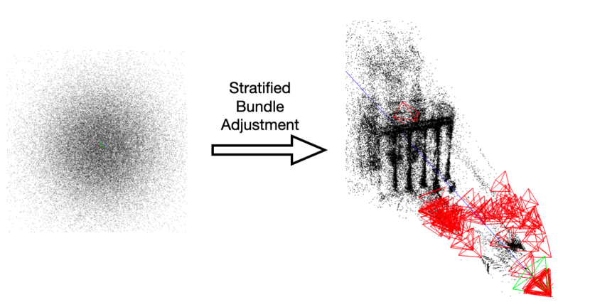
Figure 1: In contrast to traditional bundle adjustment problem, initialization-free BA is a very under-explored problem. It does not assume any approximation of pose and landmark parameters, making the problem much harder to solve. From a random initialization (left figure), and given only image measurements, we aim to recover pose and landmark parameters. Our approach, that extends inverse expansion method, is motivated by the lack of scalability of existing solvers. On the real-world BAL problems (e.g. Venice-89, right figure), we demonstrate the efficiency of the proposed combination of our novel solver Power Variable Projection (PoVar) and Riemannian manifold optimization framework for expansion method to solve the stratified BA problem.

2 Related Work

As we address the scalability of the variable projection (VarPro) algorithm for initialization-free bundle adjustment (BA), we review works on VarPro and on BA from arbitrary initialization. We also provide some background on the inverse expansion methods. A more general description of BA can be found in [23].

Variable projection (VarPro) algorithm.

VarPro is an optimization approach for solving bivariate problems that can be formulated as minimizing a cost function $f(u,v)$ with $f:\mathbb{R}^{m}\times\mathbb{R}^{n}\rightarrow\mathbb{R}$ over two sets of variables $u\in\mathbb{R}^{m}$ and $v\in\mathbb{R}^{n}$. Unlike alternation, which fixes $u$ and optimizes over $v$ and vice versa, or joint optimization, which optimizes the stack of $u$ and $v$ simultaneously, variable projection replaces $v$ with $v^{*}(u):=\operatorname*{arg\,min}_{u}f(u,v)$ ($v$ always optimal over $u$) such that the optimized cost function $f(u,v^{*}(u))=:f^{*}(u)$ becomes a function of $u$ only. The original VarPro algorithm by Golub and Pereyra [9] and its approximations by Ruhe and Wedin [20] assume solving a separable nonlinear least squares (SNLS) problem where $v^{*}(u)$ can be obtained in closed form. VarPro was consistently ignored in the computer vision community and even misidentified as a form of alternating optimization [5]. It first receives proper attention when Okatani et al. [17] demonstrates VarPro equipped with a trust-region approach such as Levenberg-Marquardt can yield a wide basin of convergence for several toy problems that can be formulated as a SNLS problem such as affine structure-from-motion and factorization-based non-rigid structure-from-motion. Shortly after, Strelow [21, 22] extends VarPro to the nonlinear case where $v^{*}(u)$ is not in closed form such as bundle adjustment. Nevertheless, these works do not address the issue of increased algorithmic complexity. Later, it has been shown by Hong et al. [12] that VarPro can be efficiently implemented by performing inner iterations [2] (also known as embedded point iterations [15]) over the set of eliminated variables $u$ followed by performing a joint optimization step with no damping on $u$. While this enables faster runtime compared to previous studies, it has only been tested up to small-medium sized problems with around 300 camera views. To this date, no work to the best of our knowledge has improved the scalability of the VarPro algorithm beyond [12].

Initialization-free bundle adjustment.

While traditional (large-scale) bundle adjustment is regularly studied ([3, 6, 26, 7, 19, 30, 4]), initialization-free BA is a recent research topic. In a seminal work, Hong et al. [13] propose to solve projective bundle adjustment from arbitrary initialization with the Variable Projection algorithm. Notably, they propose a stratified bundle adjustment formulation with increasing difficulty. In a follow-up work, pOSE [11] incorporates the equivalence between nonlinear VarPro and the Schur complement recently identified in [12]. Additionally, they define an objective in-between affine and projective models that leads to a wide convergence bassin. Iglesias et al. [14] complements this pseudo object space error formulation with an exponential regularization term, and show interesting results on very-small-scale problems. Nevertheless, up to our knowledge, none of these studies look closely into the scalability of the proposed frameworks for initialization-free bundle adjustment.

Inverse expansion method.

Despite its short recent appearance in the literature, inverse expansion method is a highly efficient and competitive approach for solving the linearized system of equations for bundle adjustment that is already challenging established factorization and iterative methods. It links the Schur complement [28] to the power series expansion of its inverse. Using the power Schur complement as a preconditioner for normal equations leads to very good results for physics problems such that convection-diffusion [29]. PoBA [25] proposes to directly apply the power Schur complement to the right-hand side of the reduced camera system. Their solver results in improved speed and accuracy for traditional bundle adjustment formulation with respect to the existing methods.

3 Problem Statement and Motivation

We consider a typical form of bundle adjustment. Given observations $m_{ij}$ for pose $i$ and landmark $j$, $K_{i}$, $R_{i}\in\,SO(3)$, $t_{i}\in\mathbb{R}^{3}$ the intrinsics, rotation and translation of pose $i$, and $x_{j}\in\mathbb{R}^{3}$,$\tilde{x}_{j}\in\,S^{4}$ the inhomogeneous and homogeneous landmark 3D positions (where $S^{n}$ denotes the set of all vectors on the unit $n$-sphere), we aim to solve:

$$\min_{\{R_{i}\}\in SO(3),\{t_{i}\},\{\tilde{x}_{j}\}}\sum_{(i,j)\in\Omega}\lVert\pi(K_{i}[R_{i}|t_{i}]\tilde{x}_{j})-m_{ij}\rVert^{2}_{2}\,,$$ (1)

where $\pi$ is the perspective projection $\pi([x,y,z]^{\top}):=[x/z,y/z]^{\top}$.

Recently, Equation 1 with good initialization has been solved very efficiently with a novel inverse expansion method.

3.1 Inverse expansion method

Inverse expansion method [29, 25] relies on the expansion of the inverse of a matrix into a power series, as stated in the following proposition:

Proposition 1

Let $M$ be a $n\times n$ matrix. If the spectral radius of $M$ satisfies $\lVert M\rVert<1$, then

$$(I-M)^{-1}=\sum_{i=0}^{m}M^{i}+R\,,$$ (2)

where the error matrix

$$R=\sum_{i=m+1}^{\infty}M^{i}\,,$$ (3)

satisfies

$$\lVert R\rVert\leq\frac{\lVert M\rVert^{m+1}}{1-\lVert M\rVert}\,.$$ (4)

Given a linear approximation of Equation 1 followed by the Schur complement trick, Weber et al. [25] relies the inverse Schur complement of the Levenberg-Marquardt algorithm to its power series. They show significant improvement in terms of speed and accuracy to solve BA problem with good initialization. In addition to this empirical insights, some convergence behaviour concerning the approximated results for the BA problem are theoretically proved.

However, it is well-known in the literature (see e.g. [13]) that solving Equation 1 from arbitrary initialization is non-feasible. Hong et al. [11] override this challenge by proposing a stratified bundle adjustment problem. Let us revisit the formulation of this approach.

3.2 Initialization-free bundle adjustment

The stratified BA problem is decomposed in two minimization problems, followed by a metric upgrade. Although we consider a pinhole camera model, the first stage assumes a projective model.

3.2.1 First stage: separable nonlinear optimization with projective camera.

Given $n_{p}$ poses and $n_{l}$ landmarks, $x=(x_{p},x_{l})$ contains all the optimization variables. We mimic the camera as a projective model. For pose $i$, we consider the camera parameters $x_{p}^{i}\in\mathbb{R}^{3\times 4}$ and solve the following generic nonlinear separable problem:

$$\min_{x_{p},\tilde{x}_{l}}F(x_{p},\tilde{x}_{l})=\big{\lVert}r(x_{p},\tilde{x}_{l})\big{\rVert}_{2}^{2}=\big{\lVert}G(x_{p})\tilde{x}_{l}^{j}-z(x_{p})\big{\rVert}_{2}^{2}\,,$$ (5)

with $G(.)$ and $z(.)$ some linear operators, and the last coefficient of $\tilde{x}_{l}^{j}$ fixed to 1. For instance, pOSE [11] – extensively used in our analysis (see Supplemental), proposes the following minimization problem:

$$F_{pOSE}(x_{p},x_{l})=\sum_{(i,j)\in\Omega}\begin{Vmatrix}\sqrt{1-\eta}(x_{p}^{i,1:2}\tilde{x}_{l}^{j}-(x_{p}^{i,3}\tilde{x}_{l}^{j})m_{ij})\\ \sqrt{\eta}(x_{p}^{i,1:2}\tilde{x}_{l}^{j}-m_{ij})\end{Vmatrix}_{2}^{2}\,,$$ (6)

with $x_{p}^{i,1:2}$ and $x_{p}^{i,3}$ respectively the first two lines and the third line of $x_{p}^{i}$, and $\eta\in[0,1]$.

Hong et al. [12] argue the superiority of VarPro over joint optimization to solve the previous equation, due to the random initialization of this stage.

Second stage: projective refinement.

The cameras and landmarks parameters obtained by solving Equation 5 are refined by minimizing the projective standard objective [13] over the projective camera models in homogeneous form ($\{\tilde{x}_{p}^{i}~{}|~{}\mathrm{vec}(\tilde{x}_{p}^{i})\in\,S^{12}\}$) and the 3D landmarks in homogeneous coordinates ($\{\tilde{x}_{l}^{j}~{}|~{}\tilde{x}_{l}^{j}\in\,S^{4}\})$:

$$\sum_{(i,j)\in\Omega}\big{\lVert}\pi(\tilde{x}^{i}_{p}\tilde{x}^{j}_{l})-m_{ij}\big{\rVert}_{2}^{2}.$$ (7)

Importantly, the optimization is performed in homogeneous coordinates. Especially, Riemannian manifold optimization [1] has to be incorporated.

Metric upgrade.

The last stage is a minimization problem to enforce the projective camera matrices to satisfy $SE(3)$ properties. Note that our work mostly focuses on the first two stages. The proposed implementation for this third stage has illustrative purpose, see Figure 1. We refer the reader to Supplemental for further details.

3.3 Limitations and proposed method

In contrast to the Levenberg-Marquardt algorithm, very few solvers have been designed to efficiently solve VarPro. In practice, even the most recent works [11, 14] use a direct factorization (e.g. Cholesky decomposition, QR factorization), that is well-known to be very poorly scalable (see e.g. [3]), to solve Equation 5. In particular, we note that these works consider bundle adjustment problems with only few tens of cameras – sometimes less than ten. On the other hand, Hong and Fitzgibbon [10] show that coupling VarPro with the popular preconditioned conjugate gradients algorithm may not converge very efficiently.

We propose to build on recent inverse expansion method. We first adapt the power series expansion to the VarPro algorithm (Section 4.2). We show that the so-called PoVar efficiently solves Equation 5. Moving forward, we extend the power series expansion to Riemannian manifold optimization (Section 4.3). This new Riemannian framework, that we call RiPoBA, is necessary to use expansion method for solving Equation 7. We demonstrate that the combination of this two solvers is highly competitive (Section 5).

4 Power Variable Projection

First, let us briefly revisit the VarPro algorithm. We refer the reader to [9] for further details.

4.1 Revisited variable projection

In contrast to joint optimization, VarPro optimizes over landmark parameters and camera parameters, but in a way different from the standard alternating least squares such that landmarks are not assumed to be fixed when updating the camera parameters. It first considers Equation 5 as a nonlinear minimization problem over $x_{l}$ only. Due to the separability of the equation, a closed-form solution for optimal $x_{l}^{*}(x_{p})$ is straightforward:

$$x_{l}^{*}(x_{p})=\operatorname*{arg\,min}_{\tilde{x}_{l}}\lVert G(x_{p})\tilde{x}_{l}-z(x_{p})\rVert_{2}^{2}=G(x_{p})^{{\dagger}}z(x_{p})\,,$$ (8)

with $G(x_{p})^{{\dagger}}$ the pseudo-inverse of $G(x_{p})$. Substituting $x_{l}^{*}(x_{p})$ in Equation 5 leads to the following reduced problem:

$$\min_{x_{p}}r^{*}(x_{p})=\min_{x_{p}}\lVert(G(x_{p})G^{{\dagger}}(x_{p})-I)z(x_{p})\rVert_{2}^{2}\,.$$ (9)

Following [12], Equation 9 can be solved with LM algorithm over $x_{p}$. The Jacobian of $r^{*}$ is approximated with the so-called RW2 approximation [16], that leads to the normal equation:

$$\begin{pmatrix}U_{\lambda}&&W\\ W^{\top}&&V_{0}\end{pmatrix}\begin{pmatrix}\Delta x_{p}\\ \Delta x_{l}\end{pmatrix}=-\begin{pmatrix}b_{p}\\ b_{l}\end{pmatrix}\,,$$ (10)

where

$$U_{\lambda}=J_{p}^{\top}J_{p}+\lambda D_{p}^{\top}D_{p}\,,$$ (11)

$$V_{0}=J_{l}^{\top}J_{l}\,,\quad W=J_{p}^{\top}J_{l}\,,$$ (12)

$$b_{p}=J_{p}^{\top}r^{0}\,,\quad b_{l}=J_{l}^{\top}r^{0}\,,$$ (13)

with $J_{l}$ and $J_{p}$ respectively the landmark and pose Jacobians of the original residual (Equation 5) around an equilibrium $r^{0}$, and $D_{p}$ diagonal damping matrix for pose variables. In contrast to joint optimization, only the pose Jacobian is damped in the associated Hessian. It follows that $U_{\lambda}$ is symmetric positive-definite [23], whereas $V_{0}$ is only guaranteed to be symmetric positive-semidefinite. Nevertheless, we observe $V_{0}$ is usually of full rank unless a 3D landmark is observed by few cameras with narrow baselines. By using the Schur complement trick, the update equation for VarPro becomes:

$$(U_{\lambda}-WV_{0}^{-1}W^{\top})\Delta x_{p}=b_{p}-WV_{0}^{-1}b_{l}\,.$$ (14)

Note that the Schur complement associated to VarPro:

$$S^{V}=U_{\lambda}-WV_{0}^{-1}W^{\top}\,,$$ (15)

while sharing a close structure to the Schur complement of the traditional BA problem, has a very different convergence behaviour, due to the undamped landmark Jacobian $V_{0}$.

4.2 Power series for VarPro

Inspired by Weber et al. [25], the following lemma holds, even if $V_{0}$ is only symmetric positive-semidefinite:

Lemma 1

Let $\mu$ be an eigenvalue of $U_{\lambda}^{-1}WV_{0}^{-1}W^{\top}$. Then

$$\mu\in[0,1[\,.$$ (16)

Proof

We refer the reader to the Supplemental.

It follows that the pose update $\Delta x_{p}$ in Equation 14 can be directly approximated by $x(m)$ with Proposition 1 applied to the Schur complement $S^{V}$:

$$x(m)=-\sum_{i=0}^{m}(U_{\lambda}^{-1}WV_{0}^{-1}W^{\top})^{i}U_{\lambda}^{-1}(b_{p}-WV_{0}^{-1}b_{l})\,.$$ (17)

Once the pose update is estimated, the landmark update can be derived following closed-form Equation 8 or the incremental method described in [12]. That extends the inverse expansion method to Variable Projection algorithm. The difference between both solvers is the role of the damped parameters. While it seems slight, this is enough to offer a very dissimilar convergence behaviour, as we will see in the experiments.

Before that, let investigate Riemannian manifold optimization, that is necessary to solve the second stage of the stratified BA problem. In particular, we show that we can link this framework to expansion method.

4.3 Power Riemannian manifold optimization

As the projective refinement step in Equation 7 involves both camera matrices and 3D landmarks in homogeneous forms, we exhibit local scale freedom for both camera and landmark parameters. This necessitates incorporation of the Riemannian manifold optimization framework without which the linearized system of equations is always rank-deficient and unsolvable. While a complete theoretical overview of such framework can be found in [1], we formalize Equation 7 as:

$$\operatorname*{arg\,min}_{\Delta\tilde{x}_{p},\Delta\tilde{x}_{l}}\lVert f(\tilde{x}_{p}+\Delta\tilde{x}_{p},\tilde{x}_{l}+\Delta\tilde{x}_{l})\rVert_{2}^{2},$$ (18)

where $\tilde{x}_{p}\in\mathbb{R}^{12n_{p}}$ denotes the stack of vectorized homogeneous camera parameters, $\tilde{x}_{l}\in\mathbb{R}^{4n_{l}}$ denotes the stack of homogeneous 3D landmarks and $\Delta\tilde{x}_{p}\in\mathbb{R}^{12n_{p}}$ and $\Delta\tilde{x}_{l}\in\mathbb{R}^{4n_{l}}$ are the updates in homogeneous camera parameters and 3D landmarks respectively. The unknowns are searched in the tangent space of current $\tilde{x}=[\tilde{x}_{p}^{\top},\tilde{x}_{l}^{\top}]^{\top}$, that we note $\tilde{x}^{\perp}\in\mathbb{R}^{(12n_{p}+4n_{l})\times(11n_{p}+3n_{l})}$ such that $(\tilde{x}^{\perp})^{\top}x=0$. To simplify notations, $\tilde{x}_{p}$ is considered as a vector in this section, and $\tilde{x}_{p}^{\perp}\in\mathbb{R}^{12n_{p}\times 11n_{p}}$, $\tilde{x}_{l}^{\perp}\in\mathbb{R}^{4n_{l}\times 3n_{l}}$ are block-diagonal, each block corresponding to the associated pose $i$ and landmark $j$, respectively. The projective refinement becomes:

$$\operatorname*{arg\,min}_{\Delta\tilde{x}\perp\tilde{x}}\lVert f(\tilde{x}_{p}+\Delta\tilde{x}_{p},\tilde{x}_{l}+\Delta\tilde{x}_{l})\rVert_{2}^{2}\,.$$ (19)

By coupling Riemannian manifold optimization and LM algorithm, and according to [1], we get the following normal equation, projected onto the tangent space of $\tilde{x}$:

$$\begin{pmatrix}(\tilde{x}_{p}^{\perp})^{\top}U_{\lambda}\tilde{x}_{p}^{\perp}&&(\tilde{x}_{p}^{\perp})^{\top}W\tilde{x}_{l}^{\perp}\\ (\tilde{x}_{l}^{\perp})^{\top}W^{\top}\tilde{x}_{p}^{\perp}&&(\tilde{x}_{l}^{\perp})^{\top}V_{\lambda}\tilde{x}_{l}^{\perp}\end{pmatrix}\begin{pmatrix}\Delta x_{p}\\ \Delta x_{l}\end{pmatrix}=-\begin{pmatrix}(\tilde{x}_{p}^{\perp})^{\top}b_{p}\\ (\tilde{x}_{l}^{\perp})^{\top}b_{l}\end{pmatrix}\,.$$ (20)

where $\Delta x_{p}\in\mathbb{R}^{11n_{p}}$ and $\Delta x_{l}\in\mathbb{R}^{3n_{l}}$ are the camera update and the landmark update respectively made on the tangent space of $x$. By keeping coherent notations we can note the projected Jacobians and the projected damping parameters onto the tangent space of $x$ as:

$$\tilde{J}_{p}=J_{p}\tilde{x}_{p}^{\perp}\,,\quad\tilde{J}_{l}=J_{l}\tilde{x}_{l}^{\perp}\,,\quad\tilde{\lambda}_{p}=(\tilde{x}_{p}^{\perp})^{\top}\lambda\tilde{x}_{p}^{\perp}\,,\quad\tilde{\lambda}_{l}=(\tilde{x}_{l}^{\perp})^{\top}\lambda\tilde{x}_{l}^{\perp}\,,$$ (21)

and then Equation 20 becomes:

$$\begin{pmatrix}\tilde{U}_{\lambda}&&\tilde{W}\\ \tilde{W}^{\top}&&\tilde{V}_{\lambda}\end{pmatrix}\begin{pmatrix}\Delta x_{p}\\ \Delta x_{l}\end{pmatrix}=-\begin{pmatrix}\tilde{b}_{p}\\ \tilde{b}_{l}\end{pmatrix}\,,$$ (22)

where

$$\tilde{U}_{\lambda}=\tilde{J}_{p}^{\top}\tilde{J}_{p}+D_{p}^{\top}\tilde{\lambda}_{p}D_{p}\,,$$ (23)

$$\tilde{V}_{\lambda}=\tilde{J}_{l}^{\top}\tilde{J}_{l}+D_{l}^{\top}\tilde{\lambda}_{l}D_{l}\,,$$ (24)

$$W=\tilde{J}_{p}^{\top}\tilde{J}_{l}\,,$$ (25)

$$\tilde{b}_{p}=\tilde{J}_{p}^{\top}r^{0}\,,\quad\tilde{b}_{l}=\tilde{J}_{l}^{\top}r^{0}\,,$$ (26)

We have unified the notations of bundle adjustment with Riemannian manifold optimization. As the projection $x^{\perp}$ is full-rank, it follows that $\tilde{U}_{\tilde{\lambda}}$ and $\tilde{V}_{\tilde{\lambda}}$ are symmetric positive-definite (see Supplemental), and then the associated Riemannian Schur complement:

$$\tilde{S}=\tilde{U}_{\tilde{\lambda}}-\tilde{W}\tilde{V}_{\tilde{\lambda}}^{-1}\tilde{W}^{\top}$$ (27)

satisfies the assumption of Proposition 1:

Lemma 2

Let $\tilde{\mu}$ be an eigenvalue of $\tilde{U}_{\tilde{\lambda}}^{-1}\tilde{W}\tilde{V}_{\tilde{\lambda}}^{-1}\tilde{W}^{\top}$. Then

$$\tilde{\mu}\in[0,1[\,.$$ (28)

The power series expansion can be applied to the inverse Riemannian Schur complement:

$$\tilde{S}^{-1}\approx\sum_{i=0}^{m}(\tilde{U}_{\tilde{\lambda}}^{-1}\tilde{W}\tilde{V}_{\tilde{\lambda}}^{-1}\tilde{W}^{\top})^{i}\tilde{U}_{\tilde{\lambda}}^{-1}\,,$$ (29)

to get pose updates, and then landmark updates by back-substitution.

Finally, the homogeneous pose and landmark updates $\Delta\tilde{x}_{p}$ and $\Delta\tilde{x}_{l}$ are retrieved by back-projecting pose and landmark updates in the tangent space to the original vector space dimension as follows:

$$\Delta\tilde{x}_{p}=\tilde{x}_{p}^{\perp}\Delta x_{p}\,,\quad\Delta\tilde{x}_{l}=\tilde{x}_{l}^{\perp}\Delta x_{l}.$$

After above updates are added to the pose and landmark parameters $x$, we carry out manifold retraction by normalizing individual vectors of camera parameters and 3D landmarks to maintain their normalized homogeneous forms.

We call this projective framework Riemannian PoBA (RiPoBA), that extends PoBA [25] to the Riemannian manifold optimization framework.

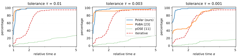
Figure 2: Performance profiles for all real-world BAL problems for solving the first stage Equation 5. Given a tolerance $\tau\in\{0.01,0.003,0.001\}$, it represents the percentage of solved problems ($y$-axis) with relative runtime $\alpha$ ($x$-axis). Expansion methods PoVar and PoBA are very competitive. Our solver PoVar is very competitive, and most notably for the highest accuracy $\tau=0.001$ and $\tau=0.003$.

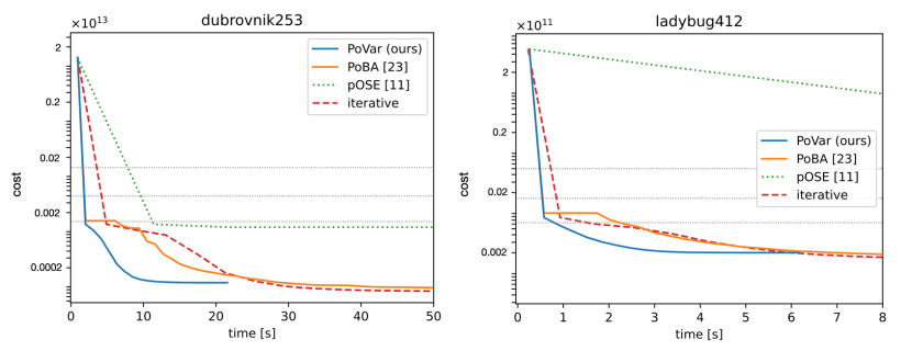
Figure 3: Convergence plots of Dubrovnik-253 (left) from BAL datasets with 253 poses and Ladybug-412 with 412 poses, for solving the first stage (Equation 5). The dotted lines correspond to cost thresholds for tolerance $\tau\in\{0.01,0.003,0.001\}$.

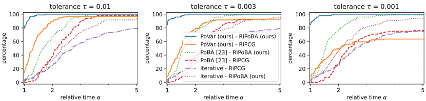
Figure 4: Performance profiles for all real-world BAL problems for solving the first two stages Equation 5 and Equation 7. In each combination, the first solver is used to solve the first stage, and the second solver is used for the second stage. Our proposed combination PoVar followed by a Riemannian expansion method outperforms by a large margin compared to all its competitors. Let emphasize that our proposed Riemannian expansion method RiPoBA outperforms the iterative baseline in all cases, given a same solver for the first stage.

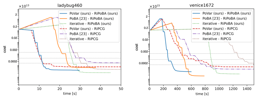
Figure 5: Convergence plots of Ladybug-460 (left) from BAL datasets with 460 poses and Venice-1672 with 1672 poses, for solving the second stage (Equation 7). The dotted lines correspond to cost thresholds for tolerance $\tau\in\{0.01,0.003,0.001\}$. Note that for fair comparison, the initial cost is derived before the first stage. The second cost – that may be higher than the initial one, is the initial cost of the second stage, after the first stage has been run. The runtime includes the time spent to solve the first stage.

5 Experiments

5.1 Implementation

We implement pOSE [11], PoVar and RiPoBA framework in C++, directly on the publicly available implementation of PoBA [25]. That leads to fair comparisons with this recent and very challenging solver. pOSE differs from PoVar by the use of a direct sparse Cholesky factorization. We also compare to VarPro with the conjugate gradients algorithm, preconditioned with Schur-Jacobi preconditioner, called iterative in our experiments. For the second stage, we compare RiPoBA to the conjugate gradients algorithm preconditioned by Schur-Jacobi preconditioners with Riemannian manifold optimization framework, called RiPCG in our experiments. Except the solver itself, all implementations share much of the code with [25]. We run experiments on MacOS 14.2.1 with an Intel Core i5 and 4 cores at 2GHz.

5.2 Experimental settings

5.2.1 Setup.

For each stage, we set the maximum number of iterations to $50$, stopping earlier if a relative function tolerance of $10^{-6}$ is achieved. The damping parameter $\lambda$ starts for each stage at $10^{-4}$ and is updated accordingly to the success or failure of the iteration. For expansion methods, we set the maximal order of power series to $20$ and a threshold to $0.01$. For iterative methods, we set the maximal number of inner iterations to $500$. We set the coefficient $\eta$ for the pOSE residuals (Equation 6) to $0.1$.

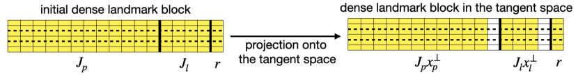
Figure 6: Example of dense landmark block in the tangent space, with three observations of the considered landmark. We project the initial dense landmark block (left figure) onto the tangent space by applying to each $i$-th pose Jacobian $J_{p_{i}}\in\mathbb{R}^{2\times 12}$ the projection $\tilde{x}_{p_{i}}^{\perp}$, and to each $j$-th landmark Jacobian $J_{l_{j}}\in\mathbb{R}^{2\times 4}$ the projection $\tilde{x}_{l_{j}}^{\perp}$. The resulting pose and landmark Jacobians in the tangent space (right figure) respectively belong to $\mathbb{R}^{2\times 11}$ and $\mathbb{R}^{2\times 3}$.

5.2.2 Efficient storage for Riemannian manifold optimization framework.

As in [25], we leverage the special structure of BA problem and propose a memory-efficient storage. We design a dense projected landmark blocks. In particular, we apply on each row associated to a landmark the block-matrices of the projection $\tilde{x}^{\perp}_{l_{j}},\tilde{x}^{\perp}_{p_{i}}$ corresponding to the landmark and to the cameras stored in the considered dense landmark block (see Figure 6).

5.2.3 Dataset.

We extensively evaluate our solver and the baselines on the $97$ real-world bundle adjustment problems from the BAL project page [3]. The number of poses goes from $16$ to $13682$. We refer the reader to Supplemental for further details about these problems. For each problem, we only keep the observation measurements. Pose parameters are randomly drawn from an isotropic Gaussian distribuaton with mean $0$ and variance $1$, and landmark parameters are deduced with Equation 8. Notably and contrary to previous works on initialization-free BA, each solver is ran on the same randomized problem, for fair comparisons.

5.3 Performance profile

To present a broad and fair analysis, we jointly evaluate both runtime and accuracy with performance profiles [8]. Given a solver, the performance profile maps the relative runtime $\alpha$ to the percentage of problems solved with accuracy $\tau$. Graphically, the performance profile of a given solver is the percentage of problems solved faster than the relative runtime $\alpha$ on the $x$-axis. Let be $S$ and $P$ the sets of solvers and problems, respectively. In practice, we can define the objective threshold for a problem $p$ by:

$$f_{\tau}(p)=f^{*}(p)+\tau(f^{0}(p)-f^{*}(p))\,,$$ (30)

with $f^{0}(p)$ the initial objective and $f^{*}(p)$ the smallest error reached by the family of solvers. The runtime a solver $s$ needs to reach this threshold is noted $T_{\tau}(p,s)$. The performance profile of a solver for a relative runtime $\alpha$ is defined as:

$$\rho(s,\alpha)=\frac{100}{\lvert P\rvert}\lvert\{p\in P|T_{\tau}(p,s)\leq\alpha\min_{s\in S}T_{\tau}(p,s)\}\lvert\,.$$ (31)

Graphically, a curve on the left of the performance profile is linked to better runtime, whereas a curve on the right is related to better accuracy. Note that for meaningful comparison, all solvers should have the same initial objective.

5.4 Analysis

5.4.1 First stage.

Figure 2 shows the performance profiles for all BAL datasets with tolerances $\tau\in\{0.01,0.003,0.001\}$ to solve Equation 5. As expected, the direct factorization solver (dashed green curve) used in Hong et al. [11] shows poor performance. Our solver PoVar (blue curve) challenges PoBA for the largest tolerance $0.01$, and is by far the most competitive solver for the smallest tolerance $\tau=0.001$, that is for the highest accuracy. For $\tau=0.003$, PoVar slightly outperforms PoBA. Let also highlight that our solver clearly outperforms the two competitors associated to the VarPro algorithm, iterative (dashed red) and direct factorization.

Figure 3 illustrates on two examples the cost decrease during the first stage. Notably, PoVar (blue curve) shows a much smoother convergence than its main challenger PoBA, that tends to stuck during the first iterations. By considering the intersections of the solvers with the cost thresholds (dashed grey lines), it also highlights the slowness of the popular iterative method compared to expansion methods, in terms of runtime.

5.4.2 First and second stage.

Figure 4 shows the performance profiles for all BAL datasets with tolerances $\tau\in\{0.01,0.003,0.001\}$ to solve the first two stages, that are Equation 5 followed by Equation 7. Note that we compare in this experiment the cost of the second stage only, as the first stage is only used to get an approximated initialization for the projective formulation. As direct factorization shows very poor performance during the first stage, we only take into account the most promising combinations of solvers. PoVar followed by RiPoBA (blue curve) clearly outperforms all the competitors with a large margin, both in terms of runtime and accuracy. The combinations with RiPoBA outperform RiPCG for the highest accuracy $\tau=0.001$ for all relative time greater than $\alpha=2$, that reflects the better convergence of Riemannian expansion method compared to RiPCG. Last but not least, given a same solver during first stage, RiPoBA clearly outperforms RiPCG during second stage, for all tolerances.

Figure 5 illustrates on two examples the cost decrease during the second stage. On the left figure, associated to Ladybug-460, the best two solvers in terms of final convergence are built on our framework RiPoBA. On the right figure, associated to Venice-1672, all the solvers using RiPoBA converge to a smaller error than their iterative competitor RiPCG. By considering the intersection between the solvers and the cost thresholds (dashed grey lines), the combination PoVar-RiPoBA clearly outperforms all the other combinations, and most notably for the largest problem with $1672$ poses.

5.4.3 Conclusive remark.

Overall, the experiments emphasize the high effectivity of our solvers PoVar and RiPoBA, during both first and second stages of the stratified BA problem. Concerning the first stage, the convergence of PoVar is much smoother than its competitors, that explains its larger speed with respect to PoBA to reach the cost thresholds, albeit both are built with power series. Regarding the second stage, for a same given solver in the first stage, our proposed RiPoBA clearly outperforms the popular preconditioned conjugate gradients with Riemannian manifold optimization framework in terms of speed and accuracy, especially when coupled with PoVar.

6 Conclusion

We introduce a novel approach to address the scalability challenge for initialization-free bundle adjustment. Our proposed Power Variable Projection (PoVar) algorithm, theoretically justified, offers new insights to this uncharted problem. By extending recent inverse expansion techniques to the VarPro algorithm on one hand, and to Riemannian manifold optimization on the other hand, we have demonstrated the capability to efficiently solve large-scale stratified BA problem with thousands of cameras. Notably, we achieve state-of-the-art results in terms of speed and accuracy on the real-world BAL dataset. While initialization-free BA is still in its nascent stage, we hope that our proposed method will pave the way for further exploration of this difficult optimization problem, and will generate further steps towards initialization-free structure-from-motion.

Power Variable Projection
for Initialization-Free Large-Scale
Bundle Adjustment
Appendix

This supplemental material is organized as follows:
Appendix 0.A studies robustness of PoVar with respect to $\eta$ and random initialization.
Appendix 0.B complements the theoretical justifications of PoVar and RiPoBA.
Appendix 0.C briefly comments a recent follow-up formulation of pOSE error.
Appendix 0.D addresses the metric upgrade stage, necessary to estimate the projective transformation and to get Euclidean reconstruction.
Appendix 0.E gives more details about the $97$ BAL problems used in our experiments.

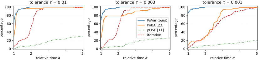
Figure 7: With $\eta=0.2$, performance profiles for all real-world BAL problems for solving the first stage (6). Given a tolerance $\tau\in\{0.01,0.003,0.001\}$, it represents the percentage of solved problems ($y$-axis) with relative runtime $\alpha$ ($x$-axis). Our solver PoVar is very competitive, and most notably for the highest accuracy $\tau=0.001$ and $\tau=0.003$.

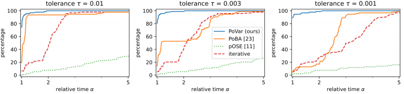
Figure 8: With $\eta=0.3$, performance profiles for all real-world BAL problems for solving the first stage (6).

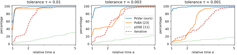
Figure 9: With $\eta=0.4$, performance profiles for all real-world BAL problems for solving the first stage (6).

Appendix 0.A Robustness

We illustrate the robustness of our solver PoVar for solving the first stage with respect to the coefficient $\eta$ in the pOSE formulation. Figure 7, Figure 8 and Figure 9 represent the performance profile for $\eta=0.2$, $\eta=0.3$ and $\eta=0.4$, respectively. We conclude that expansion methods PoBA and PoVar are both very competitive for the largest tolerance $\tau=0.01$ for all coefficients $\eta$, in line with our analysis in the main paper with $\eta=0.1$. In particular, it outperforms iterative, and direct factorization (dashed green curves) shows very poor performance due to its lack of scalability. For highest accuracy $\tau=0.003$ and $\tau=0.001$, PoVar clearly outperforms all its competitors, in line with the main paper. Note that for each $\eta$, we have randomly selected a new set of 97 problems. We can also conclude from our ablation study that our analysis is robust to random initialization.

Appendix 0.B Proof of Lemma 1

The proof in Weber et al. [23] uses the positive-definiteness of $U_{\lambda}$ and $S$ – that still holds, to show that $\mu<1$. It uses the positive-semi-definiteness of $U_{\lambda}^{-\frac{1}{2}}WV_{\lambda}^{-1}W^{\top}U_{\lambda}^{-\frac{1}{2}}$ to conclude that $\mu\geq 0$. For our VarPro formulation, we consider $V_{0}$ instead of $V_{\lambda}$. Nevertheless, it is straightforward that $U_{\lambda}^{-\frac{1}{2}}WV_{0}^{-1}W^{\top}U_{\lambda}^{-\frac{1}{2}}$ is also symmetric positive semi-definite, and then the proof stays almost the same. In details, here is the adapted proof:

Proof

On the one hand $U_{\lambda}^{-\frac{1}{2}}WV_{0}^{-1}W^{\top}U_{\lambda}^{-\frac{1}{2}}$ is symmetric positive semi-definite, as $U_{\lambda}$ is symmetric positive definite, and $V_{0}$ is symmetric positive semi-definite. Then its eigenvalues are greater than $0$. As $U_{\lambda}^{-\frac{1}{2}}WV_{0}^{-1}W^{\top}U_{\lambda}^{-\frac{1}{2}}$ and $U_{\lambda}^{-1}WV_{0}^{-1}W^{\top}$ are similar,

$$\mu\geq 0\,.$$ (32)

On the other hand $U_{\lambda}^{-\frac{1}{2}}SU_{\lambda}^{-\frac{1}{2}}$ is symmetric positive definite as $S$ and $U_{\lambda}$ are. It follows that the eigenvalues of $U_{\lambda}^{-1}S$ are all strictly positive due to its similarity with $U_{\lambda}^{-\frac{1}{2}}SU_{\lambda}^{-\frac{1}{2}}$. As

$$U_{\lambda}^{-1}WV_{0}^{-1}W^{\top}=I-U_{\lambda}^{-1}S\,,$$ (33)

it follows that

$$\mu<1\,,$$ (34)

that concludes the proof.

Concerning Riemannian manifold optimization framework, as the projection $x^{\perp}$ is full rank, it follows that $\tilde{U}_{\tilde{\lambda}}$ and $\tilde{V}_{\tilde{\lambda}}$ are symmetric positive-definite. Then, the previous proof can be very easily adapted to prove Lemma 2.

Appendix 0.C pOSE Formulation

We extensively use the pOSE formulation [11] for testing our solvers. Recently, the follow-up expOSE formulation [14] has been proposed to override some limitations of pOSE. However, such formulation raises some issues for the scalability analysis. In addition to the fact that the authors do not use the exact VarPro algorithm, expOSE requires an experimental preprocessing step over each image measurements. Without this first step, the exponential function is equal to $0$ and the algorithm does not update. Nevertheless, such preprocessing is not feasible, in terms of runtime, when the considered dataset is large enough – which is the topic of our paper, where the number of observations goes up to several tens of millions. Although interesting, expOSE is so far limited to small-scale problems, in line with the problems used by the authors – between $19$ and $30$ poses in their core paper. Extending this pseudo object space error to large-scale formulation is an interesting research direction, orthogonal to our work.

That being said, note that our proposed solver PoVar can be used for solving generic nonlinear problems, and is not restricted to the pOSE formulation.

Appendix 0.D Metric Upgrade

The third stage of pOSE [11] is the autocalibration step (see e.g. [18]), aiming to find an ambiguity matrix $H\in\mathbb{R}^{4\times 4}$ that forces the camera matrices to satisfy the $SE(3)$ constraints, that is to find $H$ such that, for all poses $i$:

$$x_{p}^{i}H=x_{p}^{i}\begin{pmatrix}A&&0\\ c^{\top}&&1\end{pmatrix}\approx K_{i}[R_{i}t_{i}]\,,$$ (35)

where $\begin{pmatrix}c^{\top}&&1\end{pmatrix}$ represents the plane at infinity. By denoting $\tilde{H}$ the three left-most columns of $H$, the $SE(3)$ constraint leads to

$$(K_{i}^{-1}x_{p}^{i})\tilde{H}\tilde{H}^{\top}(K_{i}^{-1}x_{p}^{i})^{\top}\approx I.$$ (36)

We find $c$ and the camera scales $\alpha_{i}$ by solving:

$$\min_{c,\{\alpha_{i}\}}\sum_{i=1}^{n_{p}}\lVert\alpha_{i}(K_{i}^{-1}x_{p}^{i})\tilde{H}(c)\tilde{H}(c)^{\top}(K_{i}^{-1}x_{p}^{i})^{\top}-I\rVert_{F}^{2}\,,$$ (37)

with the VarPro algorithm.

In particular, we use the chain rule and the following thorem [24]:

Theorem 0.D.1

The derivative of $\tilde{H}\tilde{H}^{\top}$ with respect to $\tilde{H}$ is equal to:

$$\frac{d\tilde{H}\tilde{H}^{\top}}{d\tilde{H}}=(I\otimes\tilde{H}^{\top})+(\tilde{H}^{\top}\otimes I)T\,,$$ (38)

where $T$ is the matrix that transforms $vec(\tilde{H})$ in $vec(\tilde{H}^{\top})$:

$$Tvec(\tilde{H})=vec(\tilde{H}^{\top})\,,$$ (39)

and $vec(H)$ is the operator that creates vector by stringing together the columns of $H$.

Appendix 0.E Dataset

Table 1: List of all 97 BAL problems [3] including number of cameras, landmarks and observations.

	cameras	landmarks	observations
ladybug-49	49	7,766	31,812
ladybug-73	73	11,022	46,091
ladybug-138	138	19,867	85,184
ladybug-318	318	41,616	179,883
ladybug-372	372	47,410	204,434
ladybug-412	412	52,202	224,205
ladybug-460	460	56,799	241,842
ladybug-539	539	65,208	277,238
ladybug-598	598	69,193	304,108
ladybug-646	646	73,541	327,199
ladybug-707	707	78,410	349,753
ladybug-783	783	84,384	376,835
ladybug-810	810	88,754	393,557
ladybug-856	856	93,284	415,551
ladybug-885	885	97,410	434,681
ladybug-931	931	102,633	457,231
ladybug-969	969	105,759	474,396
ladybug-1064	1,064	113,589	509,982
ladybug-1118	1,118	118,316	528,693
ladybug-1152	1,152	122,200	545,584
ladybug-1197	1,197	126,257	563,496
ladybug-1235	1,235	129,562	576,045
ladybug-1266	1,266	132,521	587,701
ladybug-1340	1,340	137,003	612,344
ladybug-1469	1,469	145,116	641,383
ladybug-1514	1,514	147,235	651,217
ladybug-1587	1,587	150,760	663,019
ladybug-1642	1,642	153,735	670,999
ladybug-1695	1,695	155,621	676,317
ladybug-1723	1,723	156,410	678,421
	cameras	landmarks	observations
trafalgar-21	21	11,315	36,455
trafalgar-39	39	18,060	63,551
trafalgar-50	50	20,431	73,967
trafalgar-126	126	40,037	148,117
trafalgar-138	138	44,033	165,688
trafalgar-161	161	48,126	181,861
trafalgar-170	170	49,267	185,604
trafalgar-174	174	50,489	188,598
trafalgar-193	193	53,101	196,315
trafalgar-201	201	54,427	199,727
trafalgar-206	206	54,562	200,504
trafalgar-215	215	55,910	203,991
trafalgar-225	225	57,665	208,411
trafalgar-257	257	65,131	225,698
	cameras	landmarks	observations
dubrovnik-16	16	22,106	83,718
dubrovnik-88	88	64,298	383,937
dubrovnik-135	135	90,642	552,949
dubrovnik-142	142	93,602	565,223
dubrovnik-150	150	95,821	567,738
dubrovnik-161	161	103,832	591,343
dubrovnik-173	173	111,908	633,894
dubrovnik-182	182	116,770	668,030
dubrovnik-202	202	132,796	750,977
dubrovnik-237	237	154,414	857,656
dubrovnik-253	253	163,691	898,485
dubrovnik-262	262	169,354	919,020
dubrovnik-273	273	176,305	942,302
dubrovnik-287	287	182,023	970,624
dubrovnik-308	308	195,089	1,044,529
dubrovnik-356	356	226,729	1,254,598
	cameras	landmarks	observations
venice-52	52	64,053	347,173
venice-89	89	110,973	562,976
venice-245	245	197,919	1,087,436
venice-427	427	309,567	1,695,237
venice-744	744	542,742	3,054,949
venice-951	951	707,453	3,744,975
venice-1102	1,102	779,640	4,048,424
venice-1158	1,158	802,093	4,126,104
venice-1184	1,184	815,761	4,174,654
venice-1238	1,238	842,712	4,286,111
venice-1288	1,288	865,630	4,378,614
venice-1350	1,350	893,894	4,512,735
venice-1408	1,408	911,407	4,630,139
venice-1425	1,425	916,072	4,652,920
venice-1473	1,473	929,522	4,701,478
venice-1490	1,490	934,449	4,717,420
venice-1521	1,521	938,727	4,734,634
venice-1544	1,544	941,585	4,745,797
venice-1638	1,638	975,980	4,952,422
venice-1666	1,666	983,088	4,982,752
venice-1672	1,672	986,140	4,995,719
venice-1681	1,681	982,593	4,962,448
venice-1682	1,682	982,446	4,960,627
venice-1684	1,684	982,447	4,961,337
venice-1695	1,695	983,867	4,966,552
venice-1696	1,696	983,994	4,966,505
venice-1706	1,706	984,707	4,970,241
venice-1776	1,776	993,087	4,997,468
venice-1778	1,778	993,101	4,997,555
	cameras	landmarks	observations
final-93	93	61,203	287,451
final-394	394	100,368	534,408
final-871	871	527,480	2,785,016
final-961	961	187,103	1,692,975
final-1936	1,936	649,672	5,213,731
final-3068	3,068	310,846	1,653,045
final-4585	4,585	1,324,548	9,124,880
final-13682	13,682	4,455,575	28,973,703

References

- [1] Absil, P.A., Mahony, R., Sepulchre, R.: Optimization algorithms on matrix manifolds. Princeton University Press (2008)
- [2] Agarwal, S., Mierle, K., Others: Ceres solver. http://ceres-solver.org (2024)
- [3] Agarwal, S., Snavely, N., Seitz, S.M., Szeliski, R.: Bundle adjustment in the large. In: Computer Vision–ECCV 2010: 11th European Conference on Computer Vision, Heraklion, Crete, Greece, September 5-11, 2010, Proceedings, Part II 11. pp. 29–42. Springer (2010)
- [4] Belder, A., Vivanti, R., Tal, A.: A game of bundle adjustment-learning efficient convergence. In: Proceedings of the IEEE/CVF International Conference on Computer Vision. pp. 8428–8437 (2023)
- [5] Buchanan, A.M., Fitzgibbon, A.W.: Damped Newton algorithms for matrix factorization with missing data. In: 2005 IEEE Conference on Computer Vision and Pattern Recognition (CVPR). vol. 2, pp. 316–322 (2005). https://doi.org/10.1109/CVPR.2005.118
- [6] Demmel, N., Gao, M., Laude, E., Wu, T., Cremers, D.: Distributed photometric bundle adjustment. In: 2020 International Conference on 3D Vision (3DV). pp. 140–149. IEEE (2020)
- [7] Demmel, N., Sommer, C., Cremers, D., Usenko, V.: Square root bundle adjustment for large-scale reconstruction. In: Proceedings of the IEEE/CVF Conference on Computer Vision and Pattern Recognition. pp. 11723–11732 (2021)
- [8] Dolan, E.D., Moré, J.J.: Benchmarking optimization software with performance profiles. Mathematical programming 91, 201–213 (2002)
- [9] Golub, G.H., Pereyra, V.: The differentiation of pseudo-inverses and nonlinear least squares problems whose variables separate. SIAM Journal on numerical analysis 10(2), 413–432 (1973)
- [10] Hong, J.H., Fitzgibbon, A.: Secrets of matrix factorization: Approximations, numerics, manifold optimization and random restarts. In: Proceedings of the IEEE International Conference on Computer Vision. pp. 4130–4138 (2015)
- [11] Hong, J.H., Zach, C.: pose: Pseudo object space error for initialization-free bundle adjustment. In: Proceedings of the IEEE Conference on Computer Vision and Pattern Recognition. pp. 1876–1885 (2018)
- [12] Hong, J.H., Zach, C., Fitzgibbon, A.: Revisiting the variable projection method for separable nonlinear least squares problems. In: 2017 IEEE Conference on Computer Vision and Pattern Recognition (CVPR). pp. 5939–5947. IEEE (2017)
- [13] Hong, J.H., Zach, C., Fitzgibbon, A., Cipolla, R.: Projective bundle adjustment from arbitrary initialization using the variable projection method. In: Computer Vision–ECCV 2016: 14th European Conference, Amsterdam, The Netherlands, October 11–14, 2016, Proceedings, Part I 14. pp. 477–493. Springer (2016)
- [14] Iglesias, J.P., Nilsson, A., Olsson, C.: expose: Accurate initialization-free projective factorization using exponential regularization. In: Proceedings of the IEEE/CVF Conference on Computer Vision and Pattern Recognition. pp. 8959–8968 (2023)
- [15] Jeong, Y., Nister, D., Steedly, D., Szeliski, R., Kweon, I.S.: Pushing the envelope of modern methods for bundle adjustment. In: 2010 IEEE Conference on Computer Vision and Pattern Recognition (CVPR). pp. 1474–1481 (2010). https://doi.org/10.1109/CVPR.2010.5539795
- [16] Kaufman, L.: A variable projection method for solving separable nonlinear least squares problems. BIT Numerical Mathematics 15, 49–57 (1975)
- [17] Okatani, T., Yoshida, T., Deguchi, K.: Efficient algorithm for low-rank matrix factorization with missing components and performance comparison of latest algorithms. In: 2011 IEEE International Conference on Computer Vision (ICCV). pp. 842–849 (2011). https://doi.org/10.1109/ICCV.2011.6126324
- [18] Pollefeys, M., Koch, R., Gool, L.V.: Self-calibration and metric reconstruction inspite of varying and unknown intrinsic camera parameters. International Journal of Computer Vision 32(1), 7–25 (1999)
- [19] Ren, J., Liang, W., Yan, R., Mai, L., Liu, S., Liu, X.: Megba: A gpu-based distributed library for large-scale bundle adjustment. In: European Conference on Computer Vision. pp. 715–731. Springer (2022)
- [20] Ruhe, A., Wedin, P.Å.: Algorithms for separable nonlinear least squares problems. SIAM Review (SIREV) 22(3), 318–337 (1980). https://doi.org/10.1137/1022057
- [21] Strelow, D.: General and nested Wiberg minimization. In: 2012 IEEE Conference on Computer Vision and Pattern Recognition (CVPR). pp. 1584–1591 (2012). https://doi.org/10.1109/CVPR.2012.6247850
- [22] Strelow, D.: General and nested Wiberg minimization: L2 and maximum likelihood. In: 12th European Conference on Computer Vision (ECCV). pp. 195–207 (2012). https://doi.org/10.1007/978-3-642-33786-4_15
- [23] Triggs, B., McLauchlan, P.F., Hartley, R.I., Fitzgibbon, A.W.: Bundle adjustment—a modern synthesis. In: Vision Algorithms: Theory and Practice: International Workshop on Vision Algorithms Corfu, Greece, September 21–22, 1999 Proceedings. pp. 298–372. Springer (2000)
- [24] Wang, X., Yang, W., Sun, B.: Derivatives of kronecker products themselves based on kronecker product and matrix calculus. Journal of Theoretical and Applied Information Technology 48(1) (2013)
- [25] Weber, S., Demmel, N., Chan, T.C., Cremers, D.: Power bundle adjustment for large-scale 3d reconstruction. In: Proceedings of the IEEE/CVF Conference on Computer Vision and Pattern Recognition. pp. 281–289 (2023)
- [26] Weber, S., Demmel, N., Cremers, D.: Multidirectional conjugate gradients for scalable bundle adjustment. In: DAGM German Conference on Pattern Recognition. pp. 712–724. Springer (2021)
- [27] Wright, S.J.: Numerical optimization. Springer (2006)
- [28] Zhang, F.: The Schur complement and its applications, vol. 4. Springer Science & Business Media (2006)
- [29] Zheng, Q., Xi, Y., Saad, Y.: A power schur complement low-rank correction preconditioner for general sparse linear systems. SIAM Journal on Matrix Analysis and Applications 42(2), 659–682 (2021)
- [30] Zhou, L., Luo, Z., Zhen, M., Shen, T., Li, S., Huang, Z., Fang, T., Quan, L.: Stochastic bundle adjustment for efficient and scalable 3d reconstruction. In: European Conference on Computer Vision. pp. 364–379. Springer (2020)