Towards Efficient Training and Evaluation of Robust Models against $l_{0}$ Bounded Adversarial Perturbations

Abstract

This work studies sparse adversarial perturbations bounded by $l_{0}$ norm. We propose a white-box PGD-like attack method named sparse-PGD to effectively and efficiently generate such perturbations. Furthermore, we combine sparse-PGD with a black-box attack to comprehensively and more reliably evaluate the models’ robustness against $l_{0}$ bounded adversarial perturbations. Moreover, the efficiency of sparse-PGD enables us to conduct adversarial training to build robust models against sparse perturbations. Extensive experiments demonstrate that our proposed attack algorithm exhibits strong performance in different scenarios. More importantly, compared with other robust models, our adversarially trained model demonstrates state-of-the-art robustness against various sparse attacks. Codes are available at https://github.com/CityU-MLO/sPGD.

1 Introduction

Deep learning has been developing tremendously fast in the last decade. However, it is shown vulnerable to adversarial attacks: imperceivable adversarial perturbations [1, 2] could change the prediction of a model without altering the input’s semantic content, which poses great challenges in safety-critical systems. Among different kinds of adversarial perturbations, the ones bounded by $l_{\infty}$ or $l_{2}$ norms are mostly well-studied [3, 4, 5] and benchmarked [6], because these adversarial budgets, i.e., the sets of all allowable perturbations, are convex, which facilitates theoretical analyses and algorithm design. By contrast, we study perturbations bounded by $l_{0}$ norm in this work. These perturbations are sparse and quite common in physical scenarios, including broken pixels in LED screens to fool object detection models and adversarial stickers on road signs to make an auto-driving system fail [7, 8, 9, 10, 11].

However, constructing $l_{0}$ bounded adversarial perturbations is challenging as the corresponding adversarial budget is non-convex. Therefore, gradient-based methods, such as projected gradient descent (PGD) [4], usually cannot efficiently obtain a strong adversarial perturbation. In this regard, existing methods to generate sparse perturbations [12, 13, 14, 15, 16] either cannot control the $l_{0}$ norm of perturbations or have prohibitively high computational complexity, which makes them inapplicable for adversarial training to obtain robust models against sparse perturbations. The perturbations bounded by $l_{1}$ norm are the closest scenario to sparse perturbations among convex adversarial budgets defined by an $l_{p}$ norm. Nevertheless, adversarial training in this case [17, 18] still suffers from issues such as slow convergence and instability. Jiang et al. [19] demonstrates that these issues arise from non-sparse perturbations bounded by $l_{1}$ norm. In other words, $l_{1}$ adversarial budget still cannot guarantee the sparsity of the perturbations. Thus, it is necessary to study the case of $l_{0}$ bounded perturbations.

In this work, we propose a white-box attack named sparse-PGD (sPGD) to effectively and efficiently generate sparse perturbations bounded by $l_{0}$ norm. Specifically, we decompose the sparse perturbation $\bm{\delta}$ as the product of a magnitude tensor ${\bm{p}}$ and a binary sparse mask ${\bm{m}}$: $\bm{\delta}={\bm{p}}\odot{\bm{m}}$ , where ${\bm{p}}$ and ${\bm{m}}$ determine the magnitudes and the locations of perturbed features, respectively. We adopt PGD-like algorithms to update ${\bm{p}}$ and ${\bm{m}}$. However, it is challenging to directly optimize the binary mask ${\bm{m}}$ in the discrete space. We thereby introduce an alternative continuous variable $\widetilde{{\bm{m}}}$ to approximate ${\bm{m}}$ and update $\widetilde{{\bm{m}}}$ by gradient-based methods, $\widetilde{{\bm{m}}}$ is then transformed to ${\bm{m}}$ by projection to the discrete space. Due to the sparsity of ${\bm{m}}$ by the projection operator, the gradient of ${\bm{p}}$ is sparse, which may lead to slow convergence by coordinate descent. Therefore, we can remove the projection operator in the backpropagation to obtain the unprojected gradient of ${\bm{p}}$. We use both the original sparse gradient and the unprojected gradient of ${\bm{p}}$ to boost the attack performance. Moreover, we design a random reinitialization mechanism to enhance the exploration capability for the mask ${\bm{m}}$. On top of sPGD, we propose sparse-AutoAttack (sAA), which is the ensemble of the white-box sPGD and another black-box sparse attack, for a more comprehensive and reliable evaluation against $l_{0}$ bounded perturbations. Through extensive experiments, we show that our method exhibits better performance than other attacks.

More importantly, we explore adversarial training to obtain robust models against sparse attacks. In this context, the attack method will be called in each mini-batch update, so it should be both effective and efficient. Compared with existing methods, our proposed sPGD performs much better when using a small number of iterations, making it feasible for adversarial training and its variants [20]. Empirically, models adversarially trained by sPGD demonstrate the strongest robustness against various sparse attacks.

We summarize the contributions of this paper as follows:

1. We propose an effective and efficient white-box attack algorithm named sparse-PGD (sPGD) to generate $l_{0}$ bounded adversarial perturbations.

2. sPGD achieves the best performance among white-box sparse attacks. We then combine it with a black-box sparse attack to construct sparse-AutoAttack (sAA) for more comprehensive robustness evaluation against $l_{0}$ bounded adversarial perturbations.

3. sPGD achieves much better performance in the regime of limited iterations, it is then adopted for adversarial training. Extensive experiments demonstrate that models adversarially trained by sPGD have significantly stronger robustness against various sparse attacks.

2 Preliminaries

We use image classification as an example, although the proposed methods are applicable to any classification model. Under $l_{p}$ bounded perturbations, the robust learning aims to solve the following min-max optimization problem.

$$\begin{split}\mathop{\min}\limits_{\bm{\theta}}\frac{1}{N}\sum_{i=1}^{N}\mathop{\max}\limits_{\bm{\delta}_{i}}\mathcal{L}(\bm{\theta},{\bm{x}}_{i}+\bm{\delta}_{i}),\\ \mathrm{s.t.}\ ||\bm{\delta}_{i}||_{p}\leq\epsilon,\ 0\leq{\bm{x}}_{i}+\bm{\delta}_{i}\leq 1.\end{split}$$ (1)

where $\bm{\theta}$ denotes the parameters of the model and ${\mathcal{L}}$ is the loss objective function. ${\bm{x}}_{i}\in\mathbb{R}^{h\times w\times c}$ is the input image where $h$, $w$ and $c$ represent the height, width, and number of channels, respectively. $\bm{\delta}_{i}$ has the same shape as ${\bm{x}}_{i}$ and represents the perturbation. The perturbations are constrained by its $l_{p}$ norm and the bounding box. In this regard, we use the term adversarial budget to represent the set of all allowable perturbations. Adversarial attacks focus on the inner maximization problem of (1) and aim to find the optimal adversarial perturbation, while adversarial training focuses on the outer minimization problem of (1) and aims to find a robust model parameterized by $\bm{\theta}$. Due to the high dimensionality and non-convexity of the loss function when training a deep neural network, [21] has proven that solving the problem (1) is at least NP-complete.

We consider the pixel sparsity for image inputs in this work, which is more meaningful than feature sparsity and consistent with existing works [13, 16]. That is, a pixel is considered perturbed if any of its channel is perturbed, and sparse perturbation means few pixels are perturbed.

3 Related Works

Non-Sparse Attacks: The pioneering work [1] finds the adversarial perturbations to fool image classifiers and proposes a method to minimize the $l_{2}$ norm of such perturbations. To more efficiently generate adversarial perturbations, the fast gradient sign method (FGSM) [3] generates $l_{\infty}$ perturbation in one step, but its performance is significantly surpassed by the multi-step variants [22]. Projected Gradient Descent (PGD) [4] further boosts the attack performance by using iterative updating and random initialization. Specifically, each iteration of PGD updates the adversarial perturbation $\bm{\delta}$ by:

$$\bm{\delta}\longleftarrow\Pi_{{\mathcal{S}}}(\bm{\delta}+\alpha\cdot s(\nabla_{\bm{\delta}}\mathcal{L}({\bm{\theta}},{\bm{x}}+\bm{\delta})))$$ (2)

where ${\mathcal{S}}$ is the adversarial budget, $\alpha$ is the step size, $s:\mathbb{R}^{h\times w\times c}\rightarrow\mathbb{R}^{h\times w\times c}$ selects the steepest ascent direction based on the gradient of the loss $\mathcal{L}$ with respect to the perturbation. Inspired by the first-order Taylor expansion, Madry et al. [4] derives the steepest ascent direction for $l_{2}$ bounded and $l_{\infty}$ bounded perturbations to efficiently find strong adversarial examples; SLIDE [17] and $l_{1}$-APGD [18] use $k$-coordinate ascent to construct $l_{1}$ bounded perturbations, which is shown to suffer from the slow convergence [19].

Besides the attacks that have access to the gradient of the input (i.e., white-box attacks), there are black-box attacks that do not have access to model parameters, including the ones based on gradient estimation through finite differences [23, 24, 25, 26, 27] and the ones based on evolutionary strategies or random search [28, 29]. To improve the query efficiency of these attacks, [30, 31, 32, 33] generate adversarial perturbation at the corners of the adversarial budget.

To more reliably evaluate the robustness, Croce and Hein [34] proposes AutoAttack (AA) which consists of an ensemble of several attack methods, including both black-box and white-box attacks. Croce and Hein [18] extends AA to the case of $l_{1}$ bounded perturbations and proposes AutoAttack-$l_{1}$ (AA-$l_{1}$). Although the $l_{1}$ bounded perturbations are usually sparse, Jiang et al. [19] demonstrates that AA-$l_{1}$ is able to find non-sparse perturbations that cannot be found by SLIDE to fool the models. That is to say, $l_{1}$ bounded adversarial perturbations are not guaranteed to be sparse. We should study perturbations bounded by $l_{0}$ norm.

Sparse Attacks: For perturbations bounded by $l_{0}$ norm, directly adopting vanilla PGD as in Eq. (2) leads to suboptimal performance due to the non-convexity nature of the adversarial budget: $\mathrm{PGD_{0}}$ [13], which updates the perturbation by gradient ascent and project it back to the adversarial budget, turns out very likely to trap in the local maxima. Different from $\mathrm{PGD_{0}}$, CW L0 [35] projects the perturbation onto the feasible set based on the absolute product of gradient and perturbation and adopts a mechanism similar to CW L2 [35] to update the perturbation. SparseFool [12] and GreedyFool [15] also generate sparse perturbations, but they do not strictly restrict the $l_{0}$ norm of perturbations. If we project their generated perturbations to the desired $l_{0}$ ball, their performance will drastically drop. Sparse Adversarial and Interpretable Attack Framework (SAIF) [36] is similar to our method in that SAIF also decomposes the $l_{0}$ perturbation into a magnitude tensor and sparsity mask, but it uses the Frank-Wolfe algorithm [37] to separately update them. SAIF turns out to get trapped in local minima and shows poor performance on adversarially trained models. Besides white-box attacks, there are black-box attacks to generate sparse adversarial perturbations, including CornerSearch [13] and Sparse-RS [16]. However, these black-box attacks usually require thousands of queries to find an adversarial example, making it difficult to scale up to large datasets.

Adversarial Training: Despite the difficulty in obtaining robust deep neural network, adversarial training [4, 38, 39, 40, 41, 42, 43, 44] stands out as a reliable and popular approach to do so [45, 34]. It generates adversarial examples first and then uses them to optimize model parameters. Despite effective, adversarial training is time-consuming due to multi-step attacks. Shafahi et al. [46], Zhang et al. [47], Wong et al. [48], Sriramanan et al. [49] use weaker but faster one-step attacks to reduce the overhead, but they may suffer from catastrophic overfitting [50]: the model overfits to these weak attacks during training instead of achieving true robustness to various attacks. Kim et al. [51], Andriushchenko and Flammarion [52], Golgooni et al. [53], de Jorge et al. [54] try to overcome catastrophic overfitting while maintaining efficiency.

Compared with $l_{\infty}$ and $l_{2}$ bounded perturbations, adversarial training against $l_{1}$ bounded perturbations is shown to be even more time-consuming to achieve the optimal performance [18]. In the case of $l_{0}$ bounded perturbations, PGD₀ [13] is adopted for adversarial training. However, models trained by PGD₀ exhibit poor robustness against strong sparse attacks. In this work, we propose an effective and efficient sparse attack that enables us to train a model that is more robust against various sparse attacks than existing methods.

4 Methods

In this section, we introduce sparse-PGD (sPGD): a white-box attack that generates sparse perturbations. Similar to AutoAttack [34, 18], we further combine sPGD with a black-box attack to construct sparse-AutoAttack (sAA) for more comprehensive and reliable robustness evaluation.

In the end, we incorporate sPGD into the framework of adversarial training to boost the model’s robustness against sparse perturbations.

4.1 Sparse-PGD (sPGD)

Inspired by SAIF [36], we decompose the sparse perturbation $\bm{\delta}$ into a magnitude tensor ${\bm{p}}\in\mathbb{R}^{h\times w\times c}$ and a sparsity mask ${\bm{m}}\in\{0,1\}^{h\times w\times 1}$, i.e., $\bm{\delta}={\bm{p}}\odot{\bm{m}}$. Therefore, the attacker aims to maximize the following loss objective function:

$$\max_{\|\bm{\delta}\|_{0}\leq k,0\leq{\bm{x}}+\bm{\delta}\leq 1}{\mathcal{L}}(\bm{\theta},{\bm{x}}+\bm{\delta})=\max_{{\bm{p}}\in{\mathcal{S}}_{\bm{p}},{\bm{m}}\in{\mathcal{S}}_{\bm{m}}}\mathcal{L}(\bm{\theta},{\bm{x}}+{\bm{p}}\odot{\bm{m}}).$$ (3)

The feasible sets for ${\bm{p}}$ and ${\bm{m}}$ are ${\mathcal{S}}_{\bm{p}}=\{{\bm{p}}\in\mathbb{R}^{h\times w\times c}|0\leq{\bm{x}}+{\bm{p}}\leq 1\}$ and ${\mathcal{S}}_{\bm{m}}=\{{\bm{m}}\in\{0,1\}^{h\times w\times 1}|\|{\bm{m}}\|_{0}\leq k\}$, respectively. Similar to PGD, sPGD iteratively updates ${\bm{p}}$ and ${\bm{m}}$ until finding a successful adversarial example or reaching the maximum iteration number.

Update Magnitude Tensor ${\bm{p}}$: The magnitude tensor ${\bm{p}}$ is only constrained by the input domain. In the case of images, the input is bounded between $0$ and $1$. Note that the constraints on ${\bm{p}}$ are elementwise and similar to those of $l_{\infty}$ bounded perturbations. Therefore, instead of greedy or random search [13, 16], we utilize PGD in the $l_{\infty}$ case, i.e., use the sign of the gradients, to optimize ${\bm{p}}$ as demonstrated by Eq. (4) below, with $\alpha$ being the step size.

$${\bm{p}}\longleftarrow\Pi_{{\mathcal{S}}_{{\bm{p}}}}\left({\bm{p}}+\alpha\cdot\mathtt{sign}(\nabla_{{\bm{p}}}{\mathcal{L}}(\bm{\theta},{\bm{x}}+{\bm{p}}\odot{\bm{m}}))\right),$$ (4)

Update Sparsity Mask ${\bm{m}}$: The sparsity mask ${\bm{m}}$ is binary and constrained by its $l_{0}$ norm. Directly optimizing the discrete variable ${\bm{m}}$ is challenging, so we update its continuous alternative $\widetilde{{\bm{m}}}\in\mathbb{R}^{h\times w\times 1}$ and project $\widetilde{{\bm{m}}}$ to the feasible set ${\mathcal{S}}_{\bm{m}}$ to obtain ${\bm{m}}$ before multiplying it with the magnitude tensor ${\bm{p}}$ to obtain the sparse perturbation $\bm{\delta}$. Specifically, $\widetilde{{\bm{m}}}$ is updated by gradient ascent. Projecting $\widetilde{{\bm{m}}}$ to the feasible set ${\mathcal{S}}_{{\bm{m}}}$ is to set the $k$-largest elements in $\widetilde{{\bm{m}}}$ to $1$ and the rest to $0$. In addition, we adopt the sigmoid function to normalize the elements of $\widetilde{{\bm{m}}}$ before projection.

Mathematically, the update rules for $\widetilde{{\bm{m}}}$ and ${\bm{m}}$ are demonstrated as follows:

$$\widetilde{{\bm{m}}} \longleftarrow\widetilde{{\bm{m}}}+\beta\cdot\nabla_{\widetilde{{\bm{m}}}}{\mathcal{L}}/||\nabla_{\widetilde{{\bm{m}}}}{\mathcal{L}}||_{2},$$ (5)

$${\bm{m}} \longleftarrow\Pi_{{\mathcal{S}}_{{\bm{m}}}}(\sigma(\widetilde{{\bm{m}}}))$$ (6)

where $\beta$ is the step size for updating the sparsity mask’s continuous alternative $\widetilde{{\bm{m}}}$, $\sigma(\cdot)$ denotes the sigmoid function. Furthermore, to prevent the magnitude of $\widetilde{{\bm{m}}}$ from becoming explosively large, we do not update $\widetilde{{\bm{m}}}$ when $||\nabla_{\widetilde{{\bm{m}}}}{\mathcal{L}}||_{2}<\gamma$, which indicates that $\widetilde{{\bm{m}}}$ is located in the saturation zone of sigmoid function. The gradient $\nabla_{\widetilde{{\bm{m}}}}{\mathcal{L}}$ is calculated at the point $\bm{\delta}={\bm{p}}\odot\Pi_{{\mathcal{S}}_{{\bm{m}}}}(\sigma(\widetilde{{\bm{m}}}))$, where the loss function is not always differentiable. We demonstrate how to estimate the update direction in the next part.

Backward Function: Based on Eq. (3), we can calculate the gradient of the magnitude tensor ${\bm{p}}$ by $\nabla_{\bm{p}}{\mathcal{L}}=\nabla_{\bm{\delta}}{\mathcal{L}}(\bm{\theta},{\bm{x}}+\bm{\delta})\odot{\bm{m}}$ and use $g_{{\bm{p}}}$ to represent this gradient for notation simplicity. At most, $k$ non-zero elements are in the mask ${\bm{m}}$, so $g_{\bm{p}}$ is sparse and has at most $k$ non-zero elements. That is to say, we update at most $k$ elements of the magnitude tensor ${\bm{p}}$ based on the gradient $g_{\bm{p}}$. Like coordinate descent, this may result in suboptimal performance since most elements of ${\bm{p}}$ are unchanged in each iterative update. To tackle this problem, we discard the projection to the binary set ${\mathcal{S}}_{{\bm{m}}}$ when calculating the gradient and use the unprojected gradient $\widetilde{g}_{{\bm{p}}}$ to update ${\bm{p}}$. Based on Eq. (6), we have $\widetilde{g}_{{\bm{p}}}=\nabla_{\bm{\delta}}{\mathcal{L}}(\bm{\theta},{\bm{x}}+\bm{\delta})\odot\sigma(\widetilde{{\bm{m}}})$. The idea of the unprojected gradient is inspired by training pruned neural networks and lottery ticket hypothesis [55, 56, 57, 58]. All these methods train importance scores to prune the model parameters but update the importance scores based on the whole network instead of the pruned sub-network to prevent the sparse update, which leads to suboptimal performance.

In practice, the performance of using $g_{{\bm{p}}}$ and $\widetilde{g}_{{\bm{p}}}$ to optimize ${\bm{p}}$ is complementary. The sparse gradient $g_{{\bm{p}}}$ is consistent with the forward propagation and is thus better at exploitation. By contrast, the unprojected gradient $\widetilde{g}_{{\bm{p}}}$ updates the ${\bm{p}}$ by a dense tensor and is thus better at exploration. In view of this, we set up an ensemble of attacks with both gradients to balance exploration and exploitation.

When calculating the gradient of the continuous alternative $\widetilde{{\bm{m}}}$, we have $\frac{\partial{\mathcal{L}}}{\partial\widetilde{{\bm{m}}}}=\frac{\partial{\mathcal{L}}(\theta,{\bm{x}}+\bm{\delta})}{\partial\bm{\delta}}\odot{\bm{p}}\odot\frac{\partial\Pi_{{\mathcal{S}}_{{\bm{m}}}}(\sigma(\widetilde{{\bm{m}}}))}{\partial\widetilde{{\bm{m}}}}$. Since the projection to the set ${\mathcal{S}}_{{\bm{m}}}$ is not always differentiable, we discard the projection operator and use the approximation $\frac{\partial\Pi_{{\mathcal{S}}_{{\bm{m}}}}(\sigma(\widetilde{{\bm{m}}}))}{\partial\widetilde{{\bm{m}}}}\simeq\sigma^{\prime}(\widetilde{{\bm{m}}})$ to calculate the gradient.

Algorithm 1 Sparse-PGD

1:  Input: Clean image: ${\bm{x}}\in[0,1]^{h\times w\times c}$; Model parameters: ${\bm{\theta}}$; Max iteration number: $T$; Tolerance: $t$; $l_{0}$ budget: $k$; Step size: $\alpha$, $\beta$; Small constant: $\gamma=2\times 10^{-8}$

2:  Random initialize ${\bm{p}}$ and $\widetilde{{\bm{m}}}$

3:  for $i=0,1,...,T-1$ do

4:     ${\bm{m}}=\Pi_{{\mathcal{S}}_{{\bm{m}}}}(\sigma(\widetilde{{\bm{m}}}))$

5:     Calculate the loss $\mathcal{L}({\bm{\theta}},{\bm{x}}+{\bm{p}}\odot{\bm{m}})$

6:     if unprojected then

7:        $g_{{\bm{p}}}=\nabla_{\bm{\delta}}{\mathcal{L}}\odot\sigma(\widetilde{{\bm{m}}})$       {$\bm{\delta}={\bm{p}}\odot{\bm{m}}$}

8:     else

9:        $g_{{\bm{p}}}=\nabla_{\bm{\delta}}{\mathcal{L}}\odot{\bm{m}}$

10:     end if

11:     $g_{\widetilde{{\bm{m}}}}=\nabla_{\bm{\delta}}{\mathcal{L}}\odot{\bm{p}}\odot\sigma^{\prime}(\widetilde{{\bm{m}}})$

12:     ${\bm{p}}=\Pi_{{\mathcal{S}}_{{\bm{p}}}}({\bm{p}}+\alpha\cdot\mathtt{sign}(g_{{\bm{p}}}))$

13:     ${\bm{d}}=g_{\widetilde{{\bm{m}}}}/(||g_{\widetilde{{\bm{m}}}}||_{2})$ if $||g_{\widetilde{{\bm{m}}}}||_{2}\geq\gamma$ else $0$

14:     ${\bm{m}}_{old},\ \widetilde{{\bm{m}}}={\bm{m}},\ \widetilde{{\bm{m}}}+\beta\cdot{\bm{d}}$

15:     if attack succeeds then

16:        break

17:     end if

18:     if $||\Pi_{{\mathcal{S}}_{{\bm{m}}}}(\sigma(\widetilde{{\bm{m}}}))-{\bm{m}}_{old}||_{0}\leq 0$ for $t$ consecutive iters then

19:        Random initialize $\widetilde{{\bm{m}}}$

20:     end if

21:  end for

22:  Output: Perturbation: $\bm{\delta}={\bm{p}}\odot{\bm{m}}$

Random Reinitialization: Due to the projection to the set ${\mathcal{S}}_{{\bm{m}}}$ in Eq. (6), the sparsity mask ${\bm{m}}$ changes only when the relative magnitude ordering of the continuous alternative $\widetilde{{\bm{m}}}$ changes. In other words, slight changes in $\widetilde{{\bm{m}}}$ usually mean no change in ${\bm{m}}$. As a result, ${\bm{m}}$ usually gets trapped in a local maximum. To solve this problem, we propose a random reinitialization mechanism. Specifically, when the attack fails, i.e., the model still gives the correct prediction, and the current sparsity mask ${\bm{m}}$ remains unchanged for three consecutive iterations, the continuous alternative $\widetilde{{\bm{m}}}$ will be randomly reinitialized for better exploration.

To summarize, we provide the pseudo-code of sparse PGD (sPGD) in Algorithm 1. SAIF [36] also decomposes the perturbation $\bm{\delta}$ into a magnitude tensor ${\bm{p}}$ and a mask ${\bm{m}}$, but uses a different update rule: it uses Frank-Wolfe to update both ${\bm{p}}$ and ${\bm{m}}$. By contrast, we introduce the continuous alternative $\widetilde{{\bm{m}}}$ of ${\bm{m}}$ and use gradient ascent to update ${\bm{p}}$ and $\widetilde{{\bm{m}}}$. Moreover, we include unprojected gradient and random reinitialization techniques in Algorithm 1 to further enhance the performance.

4.2 Sparse-AutoAttack (sAA)

AutoAttack (AA) [34] is an ensemble of four diverse attacks for a standardized parameters-free and reliable evaluation of robustness against $l_{\infty}$ and $l_{2}$ attacks. Croce and Hein [18] extends AutoAttack to $l_{1}$ bounded perturbations. In this work, we propose sparse-AutoAttack (sAA), which is also a parameter-free ensemble of both black-box and white-box attacks for comprehensive robustness evaluation against $l_{0}$ bounded perturbations. It can be used in a plug-and-play manner. However, different from the $l_{\infty}$, $l_{2}$ and $l_{1}$ cases, the adaptive step size, momentum and difference of logits ratio (DLR) loss function do not improve the performance in the $l_{0}$ case, so they are not adopted in sAA. In addition, compared with targeted attacks, sPGD turns out stronger when using a larger query budget in the untargeted settings given the same total number of back-propagations. As a result, we only include the untargeted sPGD with cross-entropy loss and constant step sizes in sAA. Specifically, we run sPGD twice for two different backward functions: one denoted as sPGD_proj uses the sparse gradient $g_{{\bm{p}}}$, and the other denoted as sPGD_unproj uses the unprojected gradient $\widetilde{g}_{{\bm{p}}}$ as described in Section 4.1. As for the black-box attack, we adopt the strong black-box attack Sparse-RS [16], which can generate $l_{0}$ bounded perturbations. We run each version of sPGD and Sparse-RS for $10000$ iterations, respectively. We use cascade evaluation to improve the efficiency. Concretely, suppose we find a successful adversarial perturbation by one attack for one instance. Then, we will consider the model non-robust in this instance and the same instance will not be further evaluated by other attacks. Based on the efficiency and the attack success rate, the attacks in sAA are sorted in the order of sPGD_unproj, sPGD_proj and Sparse-RS.

4.3 Adversarial Training

In addition to robustness evaluation, we also explore adversarial training to build robust models against sparse perturbations. In the framework of adversarial training, the attack is used to generate adversarial perturbation in each training iteration, so the attack algorithm should not be too computationally expensive. In this regard, we run the untargeted sPGD (Algorithm 1) for $20$ iterations to generate sparse adversarial perturbations during training. We incorporate sPGD in the framework of vanilla adversarial training [4] and TRADES [20] and name corresponding methods sAT and sTRADES, respectively. Note that we use sAT and sTRADES as two examples of applying sPGD to adversarial training, since sPGD can be incorporated into any other adversarial training variant as well. To accommodate the scenario of adversarial training, we make the following modifications to sPGD.

Random Backward Function: Since the sparse gradient and the unprojected gradient as described in Section 4.1 induce different exploration-exploitation trade-offs, we randomly select one of them to generate adversarial perturbations for each mini-batch when using sPGD to generate adversarial perturbations. Compared with mixing these two backward functions together, as in sAA, random backward function does not introduce computational overhead.

Multi-$k$ Strategy: Inspired by $l_{1}$-APGD [18] and Fast-EG-$l_{1}$ [19], multi-$k$ strategy is adopted to strengthen the robustness of model. That is, we use a larger sparsity threshold, i.e., $k$ in Algorithm 1, in the training phase than in the test phase.

Higher Tolerance for Reinitialization: The default tolerance for reinitialization in sPGD is $3$ iterations, which introduces strong stochasticity. However, in the realm of adversarial training, we have a limited number of iterations. As a result, the attacker should focus more on the exploitation ability to ensure the strength of the generated adversarial perturbations. While stochasticity introduced by frequent reinitialization hurts exploitation, we find a higher tolerance for reinitialization improves the performance. In practice, we set the tolerance to $10$ iterations in adversarial training.

5 Experiments

In this section, we conduct extensive experiments to compare our attack methods with baselines in evaluating the robustness of various models against $l_{0}$ bounded perturbations. Besides the effectiveness with an abundant query budget, we also study the efficiency of our methods when we use limited iterations to generate adversarial perturbations. Our results demonstrate that the proposed sPGD achieves the best performance among white-box attacks. When using limited iterations, sPGD achieves significantly better performance than existing methods. Therefore, sAA, consisting of the best white-box and black-box attacks, has the best attack success rate. sPGD, due to its efficiency, is utilized for adversarial training to obtain the best robust models against $l_{0}$ bounded adversarial perturbations. To further demonstrate the efficacy of our method, we evaluate the transferability of sPGD. The results show that sPGD has a high transfer success rate, making it applicable in more practical scenarios. In addition, we conduct ablation studies for analysis. The adversarial examples generated by our methods are visually interpretable and presented in Appendix C. Implementation details are deferred to Appendix B.

Table 1: Robust accuracy of various models on different attacks that generate $l_{0}$ bounded perturbations, where the sparsity level $k=20$. The models are trained on CIFAR-10. Note that we report results of Sparse-RS (RS) with fine-tuned hyperparameters, which outperforms its original version in Croce et al. [16]. CornerSearch (CS) is evaluated on $1000$ samples due to its high computational complexity.

Model	Network	Clean	Black-Box		White-Box					sAA
			CS	RS	SF	PGD0	SAIF	sPGDproj	sPGDunproj
Vanilla	RN-18	93.9	1.2	0.0	17.5	0.4	3.2	0.0	0.0	0.0
$l_{\infty}$-adv. trained, $\epsilon=8/255$
GD	PRN-18	87.4	26.7	6.1	52.6	25.2	40.4	9.0	15.6	5.3
PORT	RN-18	84.6	27.8	8.5	54.5	21.4	42.7	9.1	14.6	6.7
DKL	WRN-28	92.2	33.1	7.0	54.0	29.3	41.1	9.9	15.8	6.1
DM	WRN-28	92.4	32.6	6.7	49.4	26.9	38.5	9.9	15.1	5.9
$l_{2}$-adv. trained, $\epsilon=0.5$
HAT	PRN-18	90.6	34.5	12.7	56.3	22.5	49.5	9.1	8.5	7.2
PORT	RN-18	89.8	30.4	10.5	55.0	17.2	48.0	6.3	5.8	4.9
DM	WRN-28	95.2	43.3	14.9	59.2	31.8	59.6	13.5	12.0	10.2
FDA	WRN-28	91.8	43.8	18.8	64.2	25.5	57.3	15.8	19.2	14.1
$l_{1}$-adv. trained, $\epsilon=12$
$l_{1}$-APGD	PRN-18	80.7	32.3	25.0	65.4	39.8	55.6	17.9	18.8	16.9
Fast-EG-$l_{1}$	PRN-18	76.2	35.0	24.6	60.8	37.1	50.0	18.1	18.6	16.8
$l_{0}$-adv. trained, $k=20$
PGD0-A	PRN-18	77.5	16.5	2.9	62.8	56.0	47.9	9.9	21.6	2.4
PGD0-T	PRN-18	90.0	24.1	4.9	85.1	61.1	67.9	27.3	37.9	4.5
sAT	PRN-18	84.5	52.1	36.2	81.2	78.0	76.6	75.9	75.3	36.2
sTRADES	PRN-18	89.8	69.9	61.8	88.3	86.1	84.9	84.6	81.7	61.7

5.1 Evaluation of Different Attack Methods

First, we compare our proposed sPGD, including sPGD_proj and sPGD_unproj as defined in Section 4.2, and sAA with existing white-box and black-box attacks that generate sparse perturbations. We evaluate different attack methods based on the models trained on CIFAR-10 [59] and report the robust accuracy with $k=20$ on the whole test set in Table 1. Additionally, the results on ImageNet100 [60] and a real-world traffic sign dataset GTSRB [61] are reported in Table 2. Note that the image sizes in GTSRB vary from $15\times 15$ to $250\times 250$. For convenience, we resize them to $224\times 224$ and use the same model architecture as in ImageNet-100. Furthermore, only the training set of GTSRB has annotations, we manually split the original training set into a test set containing $1000$ instances and a new training set containing the rest data. In Appendix A.1, we report more results on CIFAR-10 with $k=10$, $k=15$, and the results of models trained on CIFAR-100 [59] in Table 7, 8, 9, respectively to comprehensively demonstrate the effectiveness of our methods.

Table 2: Robust accuracy of various models on different attacks that generate $l_{0}$ bounded perturbations. ResNet34 (RN-34) [62] is used as the network architecture. Our sAT model is trained with the sparsity level $k=1200$ and the iteration number of the attack $t=20$. (a) The models are trained on ImageNet-100 [60], and the $k$ for attacks is set to $200$. (b) The models are trained on GTSRB [61], and the $k$ for attacks is set to $600$. Note that we report results of Sparse-RS (RS) with tuned hyperparameters, which outperforms its original version in Croce et al. [16]. All methods are evaluated on $500$ samples, and CornerSearch (CS) is not evaluated here due to its high computational complexity, i.e. nearly 1 week on one GPU for each run.

Model	Network	Clean	Black-Box		White-Box					sAA
			CS	RS	SF	PGD0	SAIF	sPGDproj	sPGDunproj
Vanilla	RN-34	83.0	-	0.2	5.8	9.8	0.6	0.2	0.4	0.0
$l_{1}$-adv. trained, $\epsilon=72$
Fast-EG-$l_{1}$	RN-34	69.2	-	50.2	43.4	50.2	43.0	18.6	19.0	16.6
$l_{0}$-adv. trained, $k=200$
PGD0-A	RN-34	76.0	-	6.8	57.2	37.4	11.0	1.8	18.8	1.8
sAT	RN-34	86.2	-	61.4	84.2	83.0	69.0	78.0	77.8	61.2

(a) ImageNet, $k=200$

Model	Network	Clean	Black-Box		White-Box					sAA
			CS	RS	SF	PGD0	SAIF	sPGDproj	sPGDunproj
Vanilla	RN-34	99.9	-	18.0	18.9	63.7	9.5	0.3	0.3	0.3
$l_{0}$-adv. trained, $k=600$
PGD0-A	RN-34	99.8	-	37.6	23.6	59.8	13.8	0.0	0.0	0.0
sAT	RN-34	99.8	-	88.4	96.8	99.8	96.2	88.6	96.2	85.4

(b) GTSRB, $k=600$

Models: We select various models to comprehensively evaluate their robustness against $l_{0}$ bounded perturbations. As a baseline, we train a ResNet-18 (RN-18) [62] model on clean inputs. For adversarially trained models, we select competitive models that are publicly available, including those trained against $l_{\infty}$, $l_{2}$ and $l_{1}$ bounded perturbations. For the $l_{\infty}$ case, we include adversarial training with the generated data (GD) [41], the proxy distributions (PORT) [39], the decoupled KL divergence loss (DKL) [43] and strong diffusion models (DM) [44]. For the $l_{2}$ case, we include adversarial training with the proxy distributions (PORT) [39], strong diffusion models (DM) [44], helper examples (HAT) [42] and strong data augmentations (FDA) [40]. The $l_{1}$ case is less explored in the literature, so we only include $l_{1}$-APGD adversarial training [18] and the efficient Fast-EG-$l_{1}$ [19] for comparison. The network architecture used in these baselines is either ResNet-18 (RN-18), PreActResNet-18 (PRN-18) [63] or WideResNet-28-10 (WRN-28) [64]. For the $l_{0}$ case, we evaluate PGD₀ [13] in vanilla adversarial training (PGD₀-A) and TRADES (PGD₀-T) using the same hyper-parameter settings as in Croce and Hein [13]. Since other white-box sparse attacks present trivial performance in adversarial training, we do not include their results. Finally, we use our proposed sPGD in vanilla adversarial training (sAT) and TRADES (sTRADES) to obtain PRN-18 models to compare with these baselines.

Attacks: We compare our methods with various existing black-box and white-box attacks that generate $l_{0}$ bounded perturbations. The black-box attacks include CornerSearch (CS) [13] and Sparse-RS (RS) [16]. The white-box attacks include SparseFool (SF) [12], PGD₀ [13] and Sparse Adversarial and Interpretable Attack Framework (SAIF) [36]. The implementation details of each attack are deferred to Appendix B. Specifically, to exploit the strength of these attacks in reasonable running time, we run all these attacks for either $10000$ iterations or the number of iterations where their performances converge. Note that, the number of iterations for all these attacks are no smaller than their default settings. In addition, we report the results of RS with fine-tuned hyperparameters, which outperforms its default settings in [16]. Finally, we report the robust accuracy under CS attack based on only $1000$ random test instances due to its prohibitively high computational complexity.

Based on the results in Table 1 and Table 2, we can find that SF attack, PGD₀ attack and SAIF attack perform significantly worse than our methods for all the models studied. That is, our proposed sPGD always performs the best among white-box attacks. Among black-box attacks, CS attack can achieve competitive performance, but it runs dozens of times longer than our method does. Therefore, we focus on comparing our method with RS attack. For $l_{1}$ and $l_{2}$ models, our proposed sPGD significantly outperforms RS attack. By contrast, RS attack outperforms sPGD for $l_{\infty}$ and $l_{0}$ models. This gradient masking phenomenon is, in fact, prevalent across sparse attacks. Given sufficient iterations, RS outperforms all other existing white-box attacks for $l_{\infty}$ and $l_{0}$ models. Nevertheless, among white-box attacks, sPGD exhibits the least susceptibility to gradient masking and has the best performance. The occurrence of gradient masking in the context of $l_{0}$ bounded perturbations can be attributed to the non-convex nature of adversarial budgets. In practice, the perturbation updates often significantly deviate from the direction of the gradients because of the projection to the non-convex set. Similar to AA in the $l_{1}$, $l_{2}$ and $l_{\infty}$ cases, sAA consists of both white-box and black-box attacks for comprehensive robustness evaluation. It achieves the best performance in all cases in Table 1 and Table 2 by a considerable margin.

In the case of $l_{0}$ adversarial training, the models are adversarially trained against sparse attacks. However, Figure 1 illustrates that the performance of RS attack drastically deteriorates with limited iterations (e.g., smaller than $100$), so RS is not suitable for adversarial training where we need to generate strong adversarial perturbations in limited number iterations. Empirical evidence suggests that employing RS with $20$ iterations for adversarial training, i.e., the same number of iterations as in other methods, yields trivial performance, so it is not included in Table 1 or Table 2 for comparison. In addition, models trained by PGD₀-A and PGD₀-T, which generate $l_{0}$ bounded perturbations, exhibit poor robustness to various attack methods, especially sAA. By contrast, the models trained by sAT and sTRADES show the strongest robustness, indicated by the comprehensive sAA method and all other attack methods. Compared with sAT, sTRADES achieves better performance in both robustness and accuracy. Finally, models trained with $l_{1}$ bounded perturbations are the most robust ones among existing non-$l_{0}$ training methods. It could be attributed to the fact that $l_{1}$ norm is the tightest convex relaxation of $l_{0}$ norm [65]. From a qualitative perspective, $l_{1}$ attacks also generate relatively sparse perturbations [19], which makes the corresponding model robust to sparse perturbations to some degree.

Our results indicate sPGD and RS can complement each other. Therefore, sAA, an AutoAttack-style attack that ensembles both attacks achieves the state-of-the-art performance on all models. It is designed to have a similar computational complexity to AutoAttack in $l_{\infty}$, $l_{2}$ and $l_{1}$ cases.

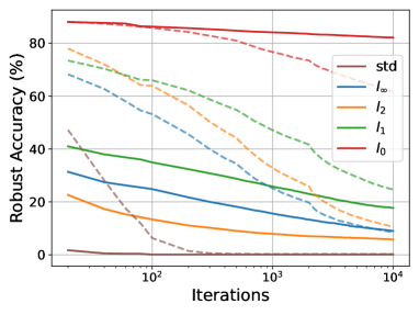
(a) CIFAR-10, $k=20$

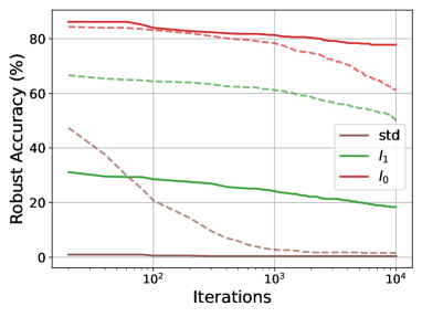
(b) ImageNet-100, $k=200$

Figure 1: Comparison between sPGD and RS attack under different iterations. (a) CIFAR-10, $k=20$. ResNet18 (std), PORT ($l_{\infty}$ and $l_{2}$) [39], $l_{1}$-APGD ($l_{1}$) [18] and sTRADES ($l_{0}$) are evaluated. (b) ImageNet-100, $k=200$. ResNet34 (std), Fast-EG-$l_{1}$ ($l_{1}$) [19] and sAT ($l_{0}$) are evaluated. The total iteration number ranges from $20$ and $10000$. The results of sPGD and RS attack are shown in solid lines and dotted lines, respectively. For better visualization, the x-axis is in the log scale.

5.2 Comparison under Different Iteration Numbers

In this subsection, we further compare our method sPGD, which is a white-box attack, with RS attack, the strongest black-box attack in the previous section. Specifically, we compare them under various iteration numbers on CIFAR-10 and ImageNet-100, which have different resolutions. Since CIFAR-100 has the same resolution as CIFAR-10, the results on CIFAR-100 are deferred to Appendix A.2. In addition, we also compare sPGD and RS under different sparsity levels in Appendix A.3.

As illustrated in Figure 1, sTRADES has better performance than other robust models by a large margin in all iterations of both sPGD and RS attacks, which is consistent with the results in Table 1, 2 and 9. For vanilla and other robust models, although the performances of both sPGD and RS attack get improved with more iterations, sPGD outperforms RS attack by a large margin when the iteration number is small (e.g. $<1000$ iterations), which makes it feasible for adversarial training. Similar to other black-box attacks, the performance of RS attack drastically deteriorates when the query budget is limited. In addition, our proposed gradient-based sPGD significantly outperforms RS on ImageNet-100, where the search space is much larger than that on CIFAR-10, i.e., higher image resolution and higher sparsity level $k$. This suggests that our approach is scalable and shows higher efficiency on high-resolution images. Furthermore, although the performance of RS does not converge even when the iteration number reaches $10000$, a larger query budget will make it computationally impractical. Following the setting in Croce et al. [16], we do not consider a larger query budget in our experiments, either. To further showcase the efficiency of our approach, we compare the distributions of the number of iterations needed by sPGD and RS to successfully generate adversarial samples and the runtime of different attacks in Appendix A.4 and A.5, respectively.

5.3 Transferability of Adversarial Perturbations

To evaluate the transferability of our attack across different models and architectures, we generate adversarial perturbations based on one model and report the attack success rate (ASR) of these perturbations on another model. As shown in Table 3, sPGD exhibits better transferability than the most competitive baseline, Sparse-RS (RS) [16]. This further demonstrates the effectiveness of our method and its potential application in more practical scenarios.

Table 3: Transferability of RS and sPGD between between VGG11 (V) and ResNet18 (R). The results are reported in attack success rate (ASR). The perturbation is generated based on the source model (left), and the ASR is obtained on the target model (right). The evaluated dataset is CIFAR-10 [59], and the sparsity level $k=20$. Note that the models are trained on clean instances, and the step-size of sPGD $\alpha$ and $\beta$ are set to 0.75.

Attack	V$\rightarrow$V	V$\rightarrow$R	R$\rightarrow$R	R$\rightarrow$V
RS	53.9	28.4	33.0	37.4
sPGDproj	58.0	43.9	50.8	48.0
sPGDunproj	64.9	40.0	52.7	56.7

5.4 Ablation Studies

We conduct ablation studies in this section. We focus on CIFAR10 and the sparsity level $k=20$. Unless specified, we use the same configurations as in Table 1.

Components of sPGD: We first validate the effectiveness of each component in sPGD. The result is reported in Table 4. We observe that naively decomposing the perturbation $\bm{\delta}$ by $\bm{\delta}={\bm{p}}\odot{\bm{m}}$ and updating them separately can deteriorate the performance. By contrast, the performance significantly improves when we update the mask ${\bm{m}}$ by its continuous alternative $\widetilde{{\bm{m}}}$ and $l_{0}$ ball projection. This indicates that introducing $\widetilde{{\bm{m}}}$ greatly mitigates the challenges in optimizing discrete variables. Moreover, the results in Table 4 indicate the performance can be further improved by the random reinitialization mechanism, which encourages exploration and avoids trapping in a local optimum. In Appendix A.6, we compare the performance when we use different step sizes for the magnitude tensor ${\bm{p}}$ and the sparsity mask ${\bm{m}}$. The results in Table A.6 and A.6 of Appendix A.6 indicate that the performance of our proposed method is quite consistent under different choices of step sizes, which facilities hyper-parameter selection for practitioners.

Table 4: Ablation study of each component in sPGD_proj in terms of robust accuracy. The model is trained by Fast-EG-$l_{1}$.

Ablations	Robust Acc.
Baseline (PGD0 w/o restart)	49.4
+ Decomposition: $\bm{\delta}={\bm{p}}\odot{\bm{m}}$	58.0 (+8.6)
+ Continuous mask $\widetilde{{\bm{m}}}$	33.9 (-15.5)
+ Random reinitialization	18.1 (-31.3)

Adversarial training: We conduct preliminary exploration on adversarial training against sparse perturbations, since sPGD can be incorporated into any adversarial training variant. Table 1, 7, 8 study sAT and sTRADES, while sTRADES outperforms sAT in all cases. In addition, the training of sAT is relatively unstable in practice, so we focus on sTRADES for ablation studies in this section. We leave the design of sPGD-adapted adversarial training variants to further improve model robustness as a future work.

Table 5.4 demonstrates the performance when we use different backward functions. The policies include always using the sparse gradient (Proj.), always using the unprojected gradient (Unproj.), alternatively using both backward functions every $5$ epochs (Alter.) and randomly selecting backward functions (Rand.). The results indicate that randomly selecting backward functions has the best performance. In addition, Table 5.4 demonstrates the robust accuracy of models trained by sTRADES with different multi-$k$ strategies. The results indicate that multi-$k$ strategy helps boost the performance. The best robust accuracy is obtained when the adversarial budget for training is $6$ times larger than that for test. Furthermore, we also study the impact of different tolerances during adversarial training in Table A.7 of Appendix A.7. The results show that higher tolerance during adversarial training benefits the robustness of the model.

Table 5: Ablation study on different policies during adversarial training. The model is PRN18 trained by sTRADES with $6\times k$. The robust accuracy is obtained through sAA.

Policy	Proj.	Unproj.	Alter.	Rand.
Acc.	41.5	39.4	51.5	61.7

Table 6: Ablation study on multi-$k$ stretegy during adversarial training. The model is PRN18 trained by sTRADES with random policy. The robust accuracy is obtained through sAA.

$k$	$1\times$	$2\times$	$4\times$	$6\times$	$8\times$	$10\times$
Acc.	34.0	39.7	54.5	61.7	60.2	55.5

6 Conclusion

In this paper, we propose an effective and efficient white-box attack named sPGD to generate sparse perturbations bounded by the $l_{0}$ norm. sPGD obtains the state-of-the-art performance among white-box attacks. Based on this, we combine it with black-box attacks for more comprehensive and reliable $l_{0}$ robustness evaluation. Our proposed sPGD is particularly effective in the realm of limited iteration numbers. Due to its efficiency, we incorporate sPGD into the framework of adversarial training to obtain robust models against sparse perturbations. The models obtained by our training method demonstrate the best robust accuracy.

7 Limitations

During adversarial training, we adopt 20-iter sPGD to generate adversarial examples, so the computational overhead is still high, making it difficult to scale up to super-large datasets. Our subsequent work will focus on developing a faster adversarial training method against $l_{0}$ bounded perturbations without sacrificing its robustness. Furthermore, since our method is evaluated on benchmarks, we do not see it has an obvious negative societal impact.

Appendix A Additional Experiments

A.1 Results of Different Sparsity Levels and Different Datasets

In this subsection, we present the robust accuracy on CIFAR-10 with the sparsity level $k=10$ and $k=15$, those on CIFAR-100 with $k=10$, those on ImageNet-100 [60] with $k=200$ and those on GTSRB [61] in Table 7, 8 and 9, respectively. It should be noted that since only the training set of GTSRB has annotations, we manually split the original training set into a training set and test set ($1000$ instances). The observations with different sparsity levels and on different datasets are consistent with those in Table 1, which indicates the effectiveness of our method.

Table 7: Robust accuracy of various models on different attacks that generate $l_{0}$ bounded perturbations, where the sparsity level $k=10$. The models are trained on CIFAR-10 [59]. Note that we report results of Sparse-RS (RS) with tuned hyperparameters, which outperforms its original version in [16]. CornerSearch (CS) is evaluated on 1000 samples due to its high computational complexity.

Model	Network	Clean	Black-Box		White-Box					sAA
			CS	RS	SF	PGD0	SAIF	sPGDproj	sPGDunproj
Vanilla	RN-18	93.9	3.2	0.5	40.6	11.5	31.8	0.5	7.7	0.5
$l_{\infty}$-adv. trained, $\epsilon=8/255$
GD	PRN-18	87.4	36.8	24.5	69.9	50.3	63.0	31.0	37.3	23.2
PORT	RN-18	84.6	36.7	27.5	70.7	46.1	62.6	31.0	36.2	25.0
DKL	WRN-28	92.2	40.9	25.0	71.9	54.2	64.6	32.6	38.8	23.7
DM	WRN-28	92.4	38.7	23.7	68.7	52.7	62.5	31.2	37.4	22.6
$l_{2}$-adv. trained, $\epsilon=0.5$
HAT	PRN-18	90.6	47.3	40.4	74.6	53.5	71.4	37.3	36.7	34.5
PORT	RN-18	89.8	46.8	37.7	74.2	50.4	70.9	33.7	33.0	30.6
DM	WRN-28	95.2	57.8	47.9	78.3	65.5	80.9	47.1	48.2	43.1
FDA	WRN-28	91.8	55.0	49.4	79.6	58.6	77.5	46.7	49.0	43.8
$l_{1}$-adv. trained, $\epsilon=12$
$l_{1}$-APGD	PRN-18	80.7	51.4	51.1	74.3	60.7	68.1	47.2	47.4	45.9
Fast-EG-$l_{1}$	PRN-18	76.2	49.7	48.0	69.7	56.7	63.2	44.7	45.0	43.2
$l_{0}$-adv. trained, $k=10$
PGD0-A	PRN-18	85.8	20.7	16.1	77.1	66.1	68.7	33.5	36.2	15.1
PGD0-T	PRN-18	90.6	22.1	14.0	85.2	72.1	76.6	37.9	44.6	13.9
sAT	PRN-18	86.4	61.0	57.4	84.1	82.0	81.1	78.2	77.6	57.4
sTRADES	PRN-18	89.8	74.7	71.6	88.8	87.7	86.9	85.9	84.5	71.6

Table 8: Robust accuracy of various models on different attacks that generate $l_{0}$ bounded perturbations, where the sparsity level $k=15$. The models are trained on CIFAR-10 [59]. Note that we report results of Sparse-RS (RS) with tuned hyperparameters, which outperforms its original version in [16]. CornerSearch (CS) is evaluated on 1000 samples due to its high computational complexity.

Model	Network	Clean	Black-Box		White-Box					sAA
			CS	RS	SF	PGD0	SAIF	sPGDproj	sPGDunproj
Vanilla	RN-18	93.9	1.6	0.0	25.3	2.1	12.0	0.0	0.0	0.0
$l_{\infty}$-adv. trained, $\epsilon=8/255$
GD	PRN-18	87.4	30.5	12.2	61.1	36.0	51.3	17.1	24.3	11.3
PORT	RN-18	84.6	30.8	15.2	62.1	31.4	52.1	17.4	23.0	13.0
DKL	WRN-28	92.2	35.3	13.2	62.5	41.2	52.3	18.4	24.9	12.1
DM	WRN-28	92.4	34.8	12.6	57.9	38.5	49.4	17.9	24.0	11.6
$l_{2}$-adv. trained, $\epsilon=0.5$
HAT	PRN-18	90.6	38.9	23.5	65.3	35.4	60.2	19.0	18.6	16.6
PORT	RN-18	89.8	36.8	20.6	64.3	30.6	59.7	16.0	15.5	13.8
DM	WRN-28	95.2	48.5	27.7	68.2	47.5	70.9	25.0	26.7	22.1
FDA	WRN-28	91.8	47.8	31.1	71.8	40.1	68.2	28.0	31.4	25.5
$l_{1}$-adv. trained, $\epsilon=12$
$l_{1}$-APGD	PRN-18	80.7	41.3	36.5	70.3	50.5	62.3	30.4	31.3	29.0
Fast-EG-$l_{1}$	PRN-18	76.2	40.7	34.8	64.9	46.7	56.9	29.6	30.1	28.0
$l_{0}$-adv. trained, $k=15$
PGD0-A	PRN-18	83.7	17.5	6.1	73.7	62.9	60.5	19.4	27.5	5.6
PGD0-T	PRN-18	90.5	19.5	7.2	85.5	63.6	69.8	31.4	41.2	7.1
sAT	PRN-18	80.9	46.0	37.6	77.1	74.1	72.3	71.2	70.3	37.6
sTRADES	PRN-18	90.3	71.7	63.7	89.5	88.1	86.5	85.9	83.8	63.7

Table 9: Robust accuracy of various models on different attacks that generate $l_{0}$ bounded perturbations, where the sparsity level $k=10$. The models are trained on CIFAR-100 [59]. Note that we report results of Sparse-RS (RS) with tuned hyperparameters, which outperforms its original version in [16]. CornerSearch (CS) is evaluated on 1000 samples due to its high computational complexity.

Model	Network	Clean	Black-Box		White-Box					sAA
			CS	RS	SF	PGD0	SAIF	sPGDproj	sPGDunproj
Vanilla	RN-18	74.3	1.6	0.3	20.1	1.9	9.0	0.1	0.9	0.1
$l_{\infty}$-adv. trained, $\epsilon=8/255$
HAT	PRN-18	61.5	12.6	9.3	39.1	19.1	26.8	11.6	14.2	8.5
FDA	PRN-18	56.9	16.3	12.3	42.2	23.0	30.7	14.9	17.8	11.6
DKL	WRN-28	73.8	12.4	6.3	44.9	20.9	26.5	10.5	14.0	6.1
DM	WRN-28	72.6	14.0	8.2	46.2	23.4	29.8	12.7	15.8	8.0
$l_{1}$-adv. trained, $\epsilon=6$
$l_{1}$-APGD	PRN-18	63.2	22.7	22.1	47.7	33.0	43.5	19.7	20.3	18.5
Fast-EG-$l_{1}$	PRN-18	59.4	21.5	21.0	44.8	30.6	39.5	18.9	18.6	17.3
$l_{0}$-adv. trained, $k=10$
PGD0-A	PRN-18	66.1	9.3	7.1	57.9	29.9	39.5	13.9	20.4	6.5
PGD0-T	PRN-18	70.7	14.8	10.5	63.5	46.3	51.7	24.5	28.6	10.2
sAT	PRN-18	67.0	44.3	41.6	65.9	61.6	60.9	56.8	58.0	41.6
sTRADES	PRN-18	70.9	52.8	50.3	69.2	67.2	65.2	64.0	63.7	50.2

A.2 Comparison under Different Iterations on CIFAR-100

Similar to the observation in Section 5.2, Figure 3 also indicates that our method can obtain a higher attack success rate than the strong black-box attack Sparse-RS (RS) when the query budget is limited. Compared with the observation in Figure 1, the efficiency of RS, which is based on heuristic random search, improves when the search space becomes smaller, i.e., smaller image space and lower sparsity level $k$.

A.3 Comparison under Different Sparsity Levels

In this subsection, we compare our method sPGD with RS attack. Specifically, we compare these two attacks under different sparsity levels, i.e., the values of $k$. We can observe from Figure 3 that RS attack shows slightly better performance only on the $l_{\infty}$ model and when $k$ is small. The search space for the perturbed features is relatively small when $k$ is small, which facilitates heuristic black-box search methods like RS attack. As $k$ increases, sPGD outperforms RS attack in all cases until both attacks achieve almost $100\%$ attack success rate.

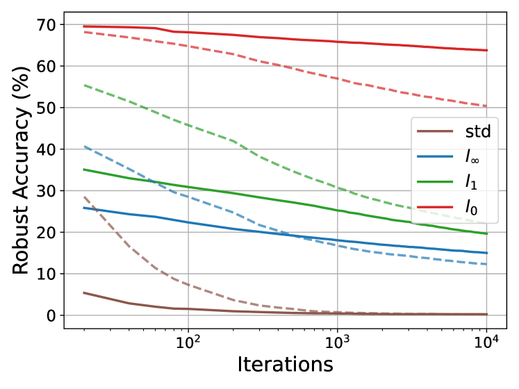
Figure 2: Comparison between sPGD and RS attack under different iterations on CIFAR-100 with $k=10$. ResNet18 (std), FDA ($l_{\infty}$) [40], $l_{1}$-APGD ($l_{1}$) [18] and sTRADES ($l_{0}$) are evaluated. The total iteration number ranges from $20$ and $10000$. The results of sPGD and RS attack are shown in solid lines and dotted lines, respectively. The x-axis is shown in the log scale.

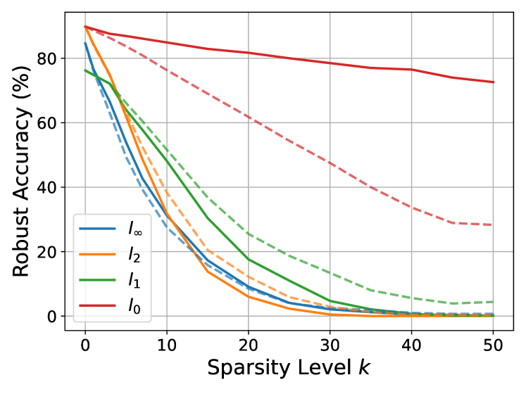
Figure 3: Comparison between sPGD and RS attack under different sparsity levels. PORT ($l_{\infty}$ and $l_{2}$) [39], $l_{1}$-APGD ($l_{1}$) [18] and sTRADES ($l_{0}$) are evaluated. The $k$ ranges from $0$ and $50$. The number of total iterations is set to $10000$. The results of sPGD and RS attack are shown in solid lines and dotted lines, respectively.

A.4 Iteration Numbers Needed to Successfully Generate Adversarial Samples

Figure 4 illustrates the distribution of the iteration numbers needed by sPGD and RS to successfully generate adversarial samples. For $l_{\infty}$, $l_{2}$ and $l_{1}$ robust models, our proposed sPGD consumes distinctly fewer iteration numbers to successfully generate an adversarial sample than RS, the strongest black-box attack in Table 1, while maintaining a high attack success rate. Similar to the observations in Figure 1, the model trained by sTRADES suffers from gradient masking. However, RS still requires a large query budget to successfully generate an adversarial sample. This further demonstrates the efficiency of sPGD, which makes it feasible for adversarial training.

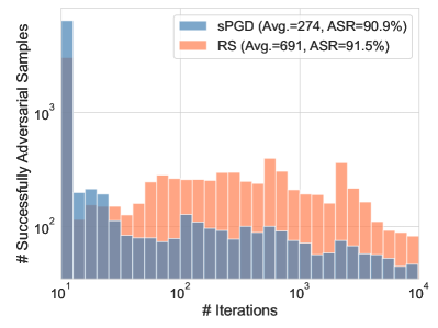
(a) $l_{\infty}$ PORT [39]

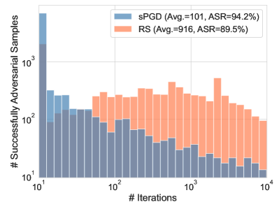
(b) $l_{2}$ PORT [39]

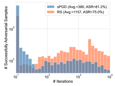
(c) $l_{1}$-APGD [18]

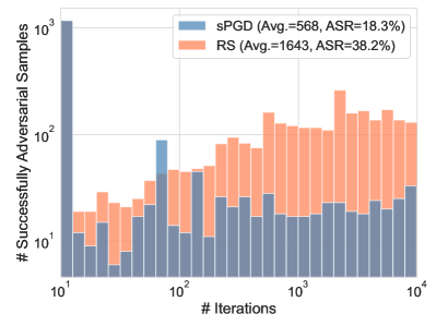
(d) sTRADES

Figure 4: Distribution of the iteration numbers needed by sPGD (blue) and RS (orange) to successfully generate adversarial samples. The results are obtained from different models: (a) $l_{\infty}$ PORT [39], (b) $l_{2}$ PORT [39], (c) $l_{1}$-APGD [18] and (d) our sPGD. The average iteration numbers (Avg.) and attack success rate (ASR), i.e., $1-$Robust Acc., are reported in the legend. For better visualization, we clip the minimum iteration number to $10$ and show the x- and y-axis in log scale.

A.5 Runtime of Different Attacks

As shown in Table 10, the proposed sPGD shows the highest efficiency among various attacks. Although sAA consumes more time (approximately $2\times$ sPGD + RS), it can provide a reliable evaluation against $l_{0}$ bounded perturbation.

Table 10: Runtime of different attacks on 1000 test instances with batch size 500. The sparsity level $k=20$. The evaluated model is sTRADES. The model is trained on CIFAR-10. The experiments are implemented on NVIDIA Tesla V100.

Attack	CS	RS	SF	PGD0	SAIF	sPGDproj	sPGDunproj	sAA
Runtime	604 min	59 min	92 min	750 min	122 min	42 min	45 min	148 min

A.6 More Ablation Study on sPGD

Step Size As shown in Table A.6 and A.6, the robust accuracy does not vary significantly with different step sizes. It indicates the satisfying robustness of our method to different hyperparameter choices. In practice, We set $\alpha$ and $\beta$ to $0.25$ and $0.25\times\sqrt{h\times w}$, respectively. Note that $h$ and $w$ denote the height and width of the image, respectively, which are both $32$ in CIFAR-10.

Tolerance during Attacking As shown in Table A.7, the performance of our method remains virtually unchanged, which showcases that our approach is robust to different choices of tolerance for reinitialization.

Table 11: Robust accuracy at different step sizes $\alpha$ for magnitude $p$. The evaluated attack is sPGD_proj. The model is Fast-EG-$l_{1}$ [19] trained on CIFAR-10 [59].

$\alpha$	$\frac{1}{16}$	$\frac{1}{8}$	$\frac{1}{4}$	$\frac{1}{2}$	$\frac{3}{4}$	$1$
Acc.	19.6	18.8	18.1	18.4	18.7	19.0

Table 12: Robust accuracy at different step sizes $\beta$ for mask $m$. The evaluated attack is sPGD_proj. The model is Fast-EG-$l_{1}$ [19] trained on CIFAR-10 [59].

$\beta$	$2$	$4$	$8$	$16$	$24$	$32$
Acc.	20.0	19.3	18.1	18.4	19.4	21.0

A.7 Impact of Tolerance during Adversarial Training

We also study the impact of different tolerances for reinitialization during adversarial training. The results reported in Table A.7 indicate that higher tolerance during adversarial training significantly improves the model’s robustness against sparse attacks, and the performance reaches its best when the tolerance is set to $10$.

Table 13: Robust accuracy at different tolerance for reinitialization $t$ during attacking. The evaluated attack is sPGD_proj. The model is Fast-EG-$l_{1}$ [19] trained on CIFAR-10 [59].

$t$	1	3	5	7	10
Acc.	18.1	18.1	18.5	18.5	18.5

Table 14: Ablation study on tolerance for reinitialization $t$ during adversarial training. The model is PRN18 trained by sTRADES with $6\times k$ and tolerance $t=3$. The robust accuracy is obtained through sAA.

$t$	3	10	20
Acc.	51.7	61.7	60.0

Appendix B Implementation Details

In experiments, we mainly focus on the cases of the sparsity of perturbations $k=10,15$ and $20$, where $k=||\sum_{i=1}^{c}\bm{\delta}^{(i)}||_{0}$ or $||{\bm{m}}||_{0}$, $\bm{\delta}^{(i)}\in{\mathbb{R}}^{h\times w}$ is the $i$-th channel of perturbation $\bm{\delta}\in{\mathbb{R}}^{h\times w\times c}$, and ${\bm{m}}\in{\mathbb{R}}^{h\times w\times 1}$ is the sparsity mask in the decomposition of $\bm{\delta}={\bm{p}}\odot{\bm{m}}$, ${\bm{p}}\in{\mathbb{R}}^{h\times w\times c}$ denotes the magnitude of perturbations.

To exploit the strength of these attacks in reasonable running time, we run all these attacks for either $10000$ iterations or the number of iterations where their performances converge. More details are elaborated below.

CornerSearch [13]: For CornerSearch, we set the hyperparameters as following: $N=100,N_{iter}=3000$, where $N$ is the sample size of the one-pixel perturbations, $N_{iter}$ is the number of queries. For bot CIFAR-10 and CIFAR-100 datasets, we evaluate the robust accuracy on $1000$ test instances due to its prohibitively high computational complexity.

Sparse-RS [16]: For Sparse-RS, we set $\alpha_{\text{init}}=0.8$, which controls the set of pixels changed in each iteration. Cross-entropy loss is adopted. Following the default setting in [16], we report the results of untargeted attacks with the maximum queries up to $10000$.

SparseFool [12]: We apply SparseFool following the official implementation and use the default value of the sparsity parameter $\lambda=3$. The maximum iterations per sample is set to $3000$. Finally, the perturbation generated by SparseFool is projected to the $l_{0}$ ball to satisfy the adversarial budget.

PGD₀ [13]: For PGD₀, we include both untargeted attack and targeted attacks on the top-$9$ incorrect classes with the highest confidence scores. We set the step size to $\eta=120000/255$. Contrary to the default setting, the iteration numbers of each attack increase from $20$ to $300$. Besides, $5$ restarts are adopted to boost the performance further.

SAIF [36]: Similar to $\mathrm{PGD_{0}}$, we apply both untargeted attack and targeted attacks on the top-$9$ incorrect classes with $300$ iterations per attack, however, the query budget is only $100$ iterations in the original paper [36]. We adopt the same $l_{\infty}$ norm constraint for the magnitude tensor $p$ as in sPGD.

sparse-PGD (sPGD): Cross-entropy loss is adopted as the loss function of both untargeted and targeted versions of our method. The step size for magnitude ${\bm{p}}$ is set $\alpha=1/4$; the step size for continuous mask $\widetilde{{\bm{m}}}$ is set $\beta=1/4\times\sqrt{h\times w}$, where $h$ and $w$ are the height and width of the input image ${\bm{x}}\in{\mathbb{R}}^{h\times w\times c}$, respectively. The small constant $\gamma$ to avoid numerical error is set to $1\times 10^{-10}$. The number of iterations is $10000$ for all datasets to ensure fair comparison among attacks in Table 1. The tolerance for reinitialization is set to $3$.

sparse-AutoAttack (sAA): It is a cascade ensemble of five different attacks, i.e., a) untargeted sPGD with unprojected gradient (sPGD_unproj), b) untargeted sPGD with sparse gradient (sPGD_proj), and c) untargeted Sparse-RS. The hyper-parameters of sPGD are the same as those listed in the last paragraph.

Adversarial Training: sPGD is adopted as the attack during the training phase, the number of iterations is $20$, and the backward function is randomly selected from the two different backward functions for each batch. For sTRADES, we only compute the TRADES loss when training, and generating adversarial examples is based on cross-entropy loss. We use PreactResNet18 [63] with softplus activation [66] for experiments on CIFAR-10 and CIFAR-100 [59], and ResNet34 [62] for experiments on ImageNet100 [60]. We train the model for $100$ epochs, the training batch size is $128$. The optimizer is SGD with a momentum factor of $0.9$ and weight decay factor of $5\times 10^{-4}$. The learning rate is initialized to $0.05$ and is divided by a factor of $10$ at the $30$th epoch and the $35$th epoch. The tolerance for reinitialization is set to $10$.

Appendix C Visualization of Some Adversarial Samples

We show some adversarial examples with different sparsity levels of perturbation in Figure 5, 6, 7. The attack is sPGD, and the model is Fast-EG-$l_{1}$ [19] trained on CIFAR-10. We can observe that most of the perturbed pixels are located in the foreground of images. It is consistent with the intuition that the foreground of an image contains most of the semantic information.

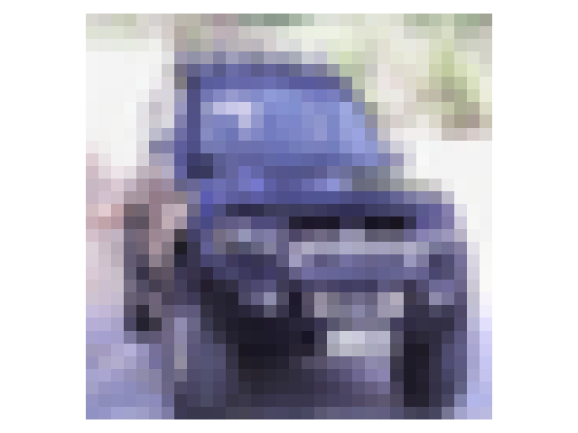
(a) automobile

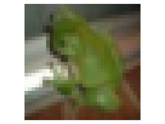
(b) frog

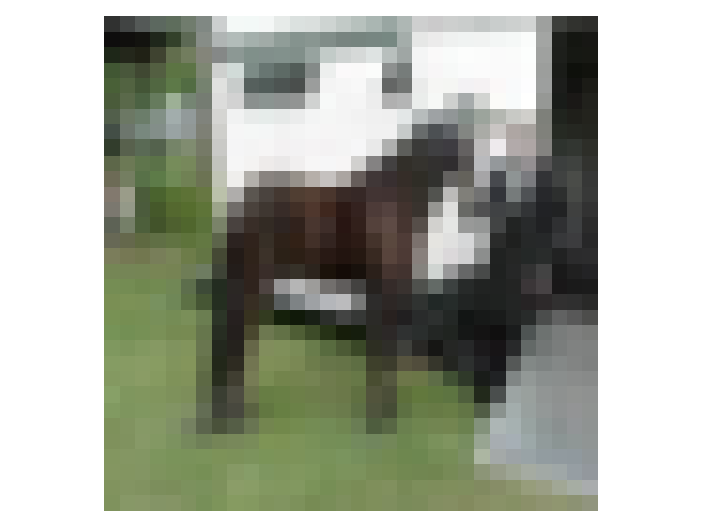
(c) horse

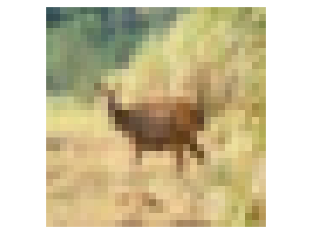
(d) deer

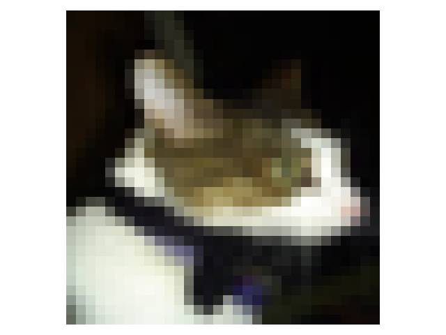
(e) cat

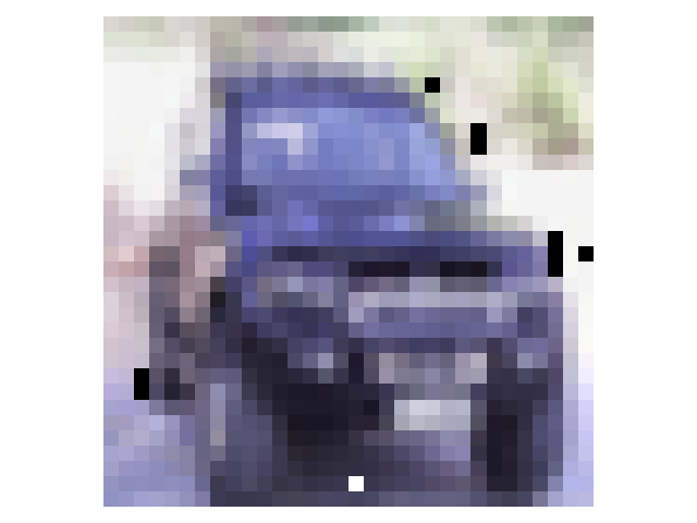
(f) truck

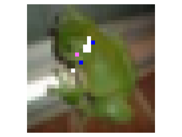
(g) deer

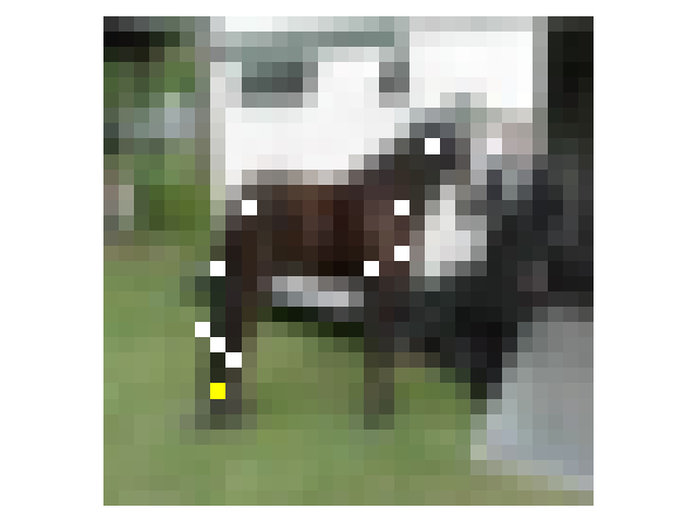
(h) automobile

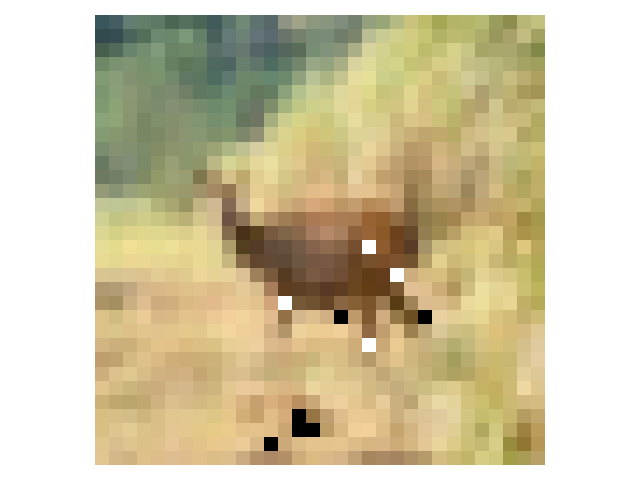
(i) bird

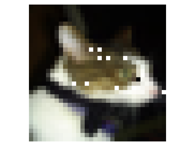
(j) ship

Figure 5: Clean images (first row) from the test set of CFIFAR-10 and their corresponding adversarial samples (second row) by sPGD. The attack is sPGD with sparsity level $k=10$. The model is Fast-EG-$l_{1}$ trained on CIFAR-10. The predictions given by the model are listed below the images.

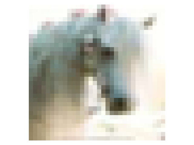
(a) horse

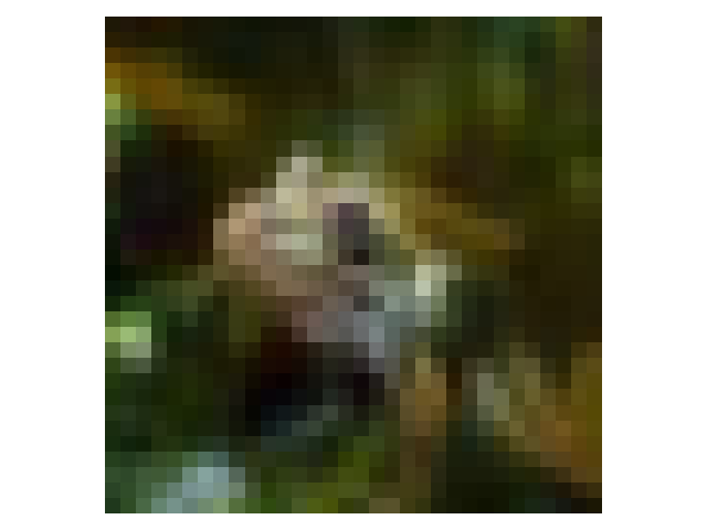
(b) frog

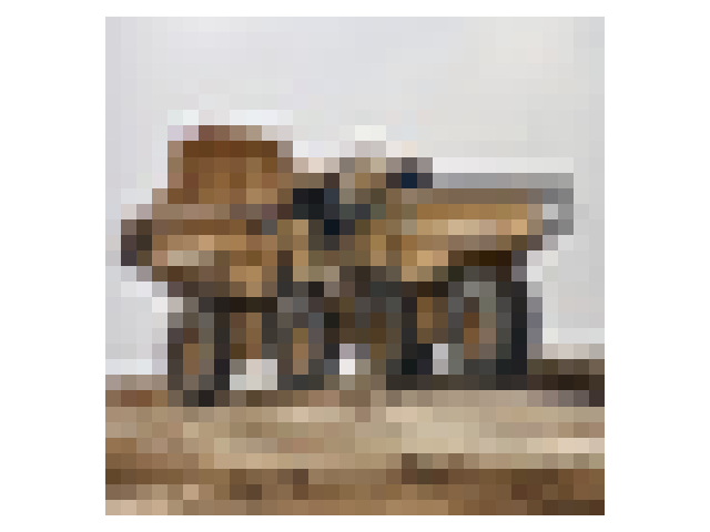
(c) truck

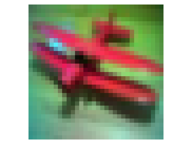
(d) airplane

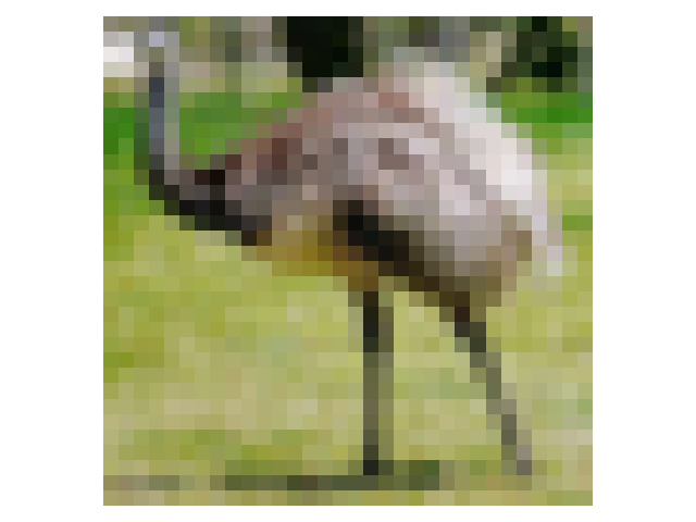
(e) bird

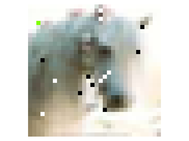
(f) cat

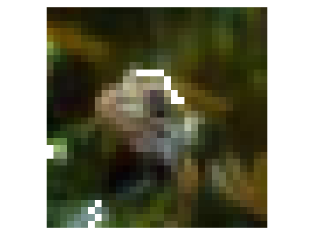
(g) bird

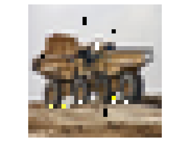
(h) horse

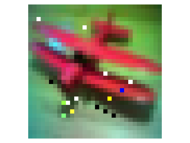
(i) automobile

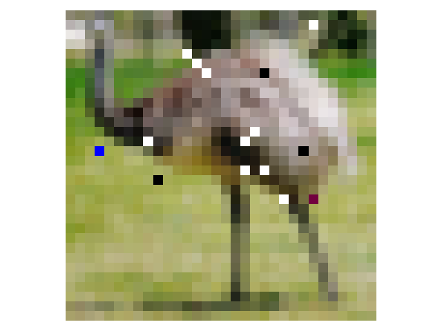
(j) horse

Figure 6: Clean images (first row) from the test set of CFIFAR-10 and their corresponding adversarial samples (second row) by sPGD. The attack is sPGD with sparsity level $k=15$. The model is Fast-EG-$l_{1}$ trained on CIFAR-10. The predictions given by the model are listed below the images.

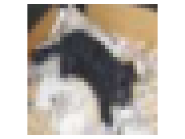
(a) dog

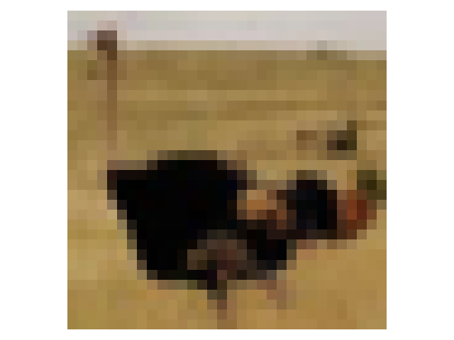
(b) bird

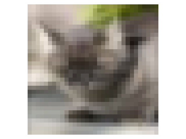
(c) cat

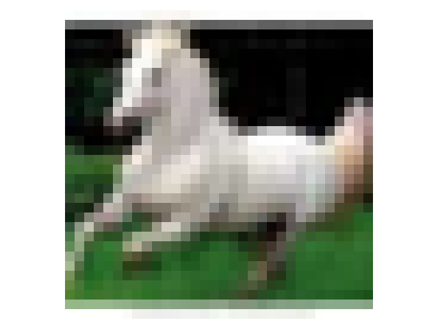
(d) horse

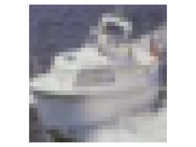
(e) ship

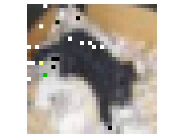
(f) cat

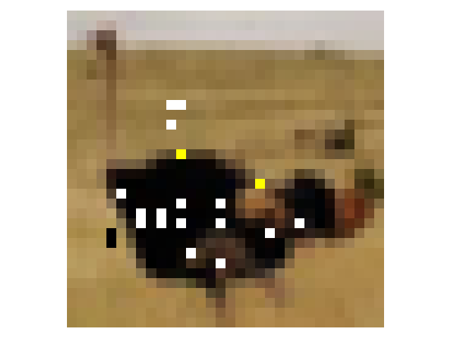
(g) automobile

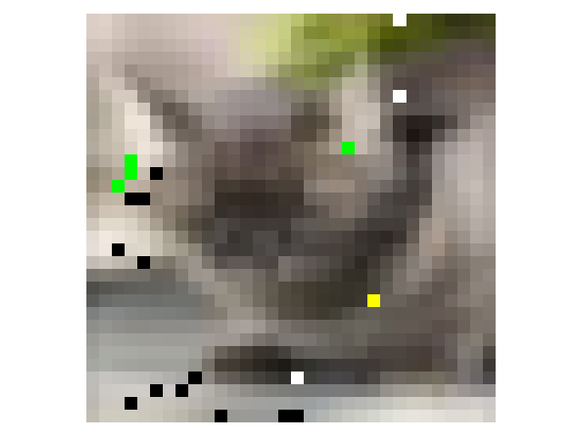
(h) bird

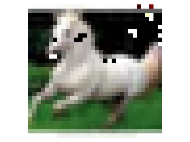
(i) dog

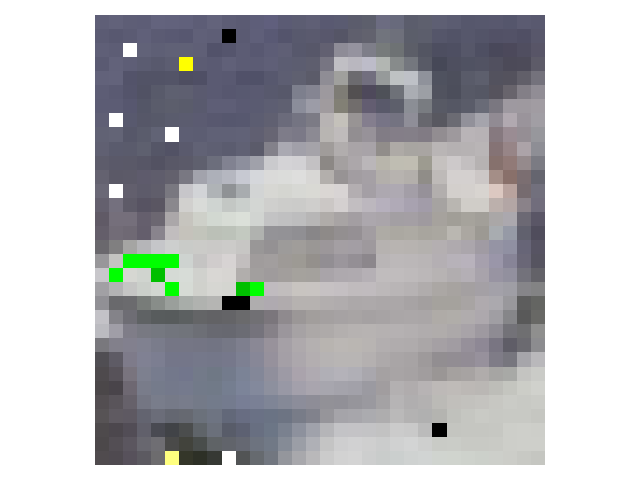
(j) cat

Figure 7: Clean images (first row) from the test set of CFIFAR-10 and their corresponding adversarial samples (second row) by sPGD. The attack is sPGD with sparsity level $k=20$. The model is Fast-EG-$l_{1}$ trained on CIFAR-10. The predictions given by the model are listed below the images.

References

- Szegedy et al. [2013] Christian Szegedy, Wojciech Zaremba, Ilya Sutskever, Joan Bruna, Dumitru Erhan, Ian Goodfellow, and Rob Fergus. Intriguing properties of neural networks. Computer Science, 2013.
- Kurakin et al. [2016] Alexey Kurakin, Ian Goodfellow, and Samy Bengio. Adversarial examples in the physical world. 2016.
- Goodfellow et al. [2014] Ian J. Goodfellow, Jonathon Shlens, and Christian Szegedy. Explaining and harnessing adversarial examples. Computer Science, 2014.
- Madry et al. [2017] Aleksander Madry, Aleksandar Makelov, Ludwig Schmidt, Dimitris Tsipras, and Adrian Vladu. Towards deep learning models resistant to adversarial attacks. arXiv preprint arXiv:1706.06083, 2017.
- Zhang et al. [2019a] Hongyang Zhang, Yaodong Yu, Jiantao Jiao, Eric P. Xing, and Michael I. Jordan. Theoretically principled trade-off between robustness and accuracy. 2019a.
- Croce et al. [2020] Francesco Croce, Maksym Andriushchenko, Vikash Sehwag, Edoardo Debenedetti, Nicolas Flammarion, Mung Chiang, Prateek Mittal, and Matthias Hein. Robustbench: a standardized adversarial robustness benchmark. arXiv preprint arXiv:2010.09670, 2020.
- Papernot et al. [2017] Nicolas Papernot, Patrick McDaniel, Ian Goodfellow, Somesh Jha, Z Berkay Celik, and Ananthram Swami. Practical black-box attacks against machine learning. In Proceedings of the 2017 ACM on Asia conference on computer and communications security, pages 506–519, 2017.
- Akhtar and Mian [2018] Naveed Akhtar and Ajmal S. Mian. Threat of adversarial attacks on deep learning in computer vision: A survey. IEEE Access, 6:14410–14430, 2018. URL https://api.semanticscholar.org/CorpusID:3536399.
- Xu et al. [2019] Han Xu, Yao Ma, Haochen Liu, Debayan Deb, Hui Liu, Jiliang Tang, and Anil K. Jain. Adversarial attacks and defenses in images, graphs and text: A review. International Journal of Automation and Computing, 17:151 – 178, 2019. URL https://api.semanticscholar.org/CorpusID:202660800.
- Feng et al. [2022] Ryan Feng, Neal Mangaokar, Jiefeng Chen, Earlence Fernandes, Somesh Jha, and Atul Prakash. Graphite: Generating automatic physical examples for machine-learning attacks on computer vision systems. In 2022 IEEE 7th European symposium on security and privacy (EuroS&P), pages 664–683. IEEE, 2022.
- Wei et al. [2023] Xingxing Wei, Yao Huang, Yitong Sun, and Jie Yu. Unified adversarial patch for cross-modal attacks in the physical world. In Proceedings of the IEEE/CVF International Conference on Computer Vision, pages 4445–4454, 2023.
- Modas et al. [2018] Apostolos Modas, Seyed Mohsen Moosavi-Dezfooli, and Pascal Frossard. Sparsefool: a few pixels make a big difference. 2018.
- Croce and Hein [2019a] Francesco Croce and Matthias Hein. Sparse and imperceivable adversarial attacks. In Proceedings of the IEEE/CVF international conference on computer vision, pages 4724–4732, 2019a.
- Su et al. [2019] Jiawei Su, Danilo Vasconcellos Vargas, and Kouichi Sakurai. One pixel attack for fooling deep neural networks. IEEE Transactions on Evolutionary Computation, 23(5):828–841, 2019.
- Dong et al. [2020] Xiaoyi Dong, Dongdong Chen, Jianmin Bao, Chuan Qin, Lu Yuan, Weiming Zhang, Nenghai Yu, and Dong Chen. Greedyfool: Distortion-aware sparse adversarial attack. 2020.
- Croce et al. [2022] Francesco Croce, Maksym Andriushchenko, Naman D Singh, Nicolas Flammarion, and Matthias Hein. Sparse-rs: a versatile framework for query-efficient sparse black-box adversarial attacks. In Proceedings of the AAAI Conference on Artificial Intelligence, volume 36, pages 6437–6445, 2022.
- Tramer and Boneh [2019] Florian Tramer and Dan Boneh. Adversarial training and robustness for multiple perturbations. Advances in neural information processing systems, 32, 2019.
- Croce and Hein [2021] Francesco Croce and Matthias Hein. Mind the box: -apgd for sparse adversarial attacks on image classifiers. In International Conference on Machine Learning, pages 2201–2211. PMLR, 2021.
- Jiang et al. [2023] Yulun Jiang, Chen Liu, Zhichao Huang, Mathieu Salzmann, and Sabine Süsstrunk. Towards stable and efficient adversarial training against bounded adversarial attacks. In International Conference on Machine Learning. PMLR, 2023.
- Zhang et al. [2019b] Hongyang Zhang, Yaodong Yu, Jiantao Jiao, Eric P. Xing, Laurent El Ghaoui, and Michael I. Jordan. Theoretically principled trade-off between robustness and accuracy. ArXiv, abs/1901.08573, 2019b. URL https://api.semanticscholar.org/CorpusID:59222747.
- Weng et al. [2018] Tsui-Wei Weng, Huan Zhang, Hongge Chen, Zhao Song, Cho-Jui Hsieh, Duane S. Boning, Inderjit S. Dhillon, and Luca Daniel. Towards fast computation of certified robustness for relu networks. ArXiv, abs/1804.09699, 2018. URL https://api.semanticscholar.org/CorpusID:13750928.
- Kurakin et al. [2017] Alexey Kurakin, Ian J. Goodfellow, and Samy Bengio. Adversarial machine learning at scale. In International Conference on Learning Representations, 2017. URL https://openreview.net/forum?id=BJm4T4Kgx.
- Bhagoji et al. [2018] Arjun Nitin Bhagoji, Warren He, Bo Li, and Dawn Xiaodong Song. Practical black-box attacks on deep neural networks using efficient query mechanisms. In European Conference on Computer Vision, 2018. URL https://api.semanticscholar.org/CorpusID:52951839.
- Ilyas et al. [2018a] Andrew Ilyas, Logan Engstrom, Anish Athalye, and Jessy Lin. Black-box adversarial attacks with limited queries and information. In International Conference on Machine Learning, 2018a. URL https://api.semanticscholar.org/CorpusID:5046541.
- Ilyas et al. [2018b] Andrew Ilyas, Logan Engstrom, and Aleksander Madry. Prior convictions: Black-box adversarial attacks with bandits and priors. ArXiv, abs/1807.07978, 2018b. URL https://api.semanticscholar.org/CorpusID:49907212.
- Tu et al. [2018] Chun-Chen Tu, Pai-Shun Ting, Pin-Yu Chen, Sijia Liu, Huan Zhang, Jinfeng Yi, Cho-Jui Hsieh, and Shin-Ming Cheng. Autozoom: Autoencoder-based zeroth order optimization method for attacking black-box neural networks. In AAAI Conference on Artificial Intelligence, 2018. URL https://api.semanticscholar.org/CorpusID:44079102.
- Uesato et al. [2018] Jonathan Uesato, Brendan O’Donoghue, Aäron van den Oord, and Pushmeet Kohli. Adversarial risk and the dangers of evaluating against weak attacks. ArXiv, abs/1802.05666, 2018. URL https://api.semanticscholar.org/CorpusID:3639844.
- Alzantot et al. [2018] Moustafa Farid Alzantot, Yash Sharma, Supriyo Chakraborty, and Mani B. Srivastava. Genattack: practical black-box attacks with gradient-free optimization. Proceedings of the Genetic and Evolutionary Computation Conference, 2018. URL https://api.semanticscholar.org/CorpusID:44166696.
- Guo et al. [2019] Chuan Guo, Jacob R. Gardner, Yurong You, Andrew Gordon Wilson, and Kilian Q. Weinberger. Simple black-box adversarial attacks. ArXiv, abs/1905.07121, 2019. URL https://api.semanticscholar.org/CorpusID:86541092.
- Al-Dujaili and O’Reilly [2019] Abdullah Al-Dujaili and Una-May O’Reilly. There are no bit parts for sign bits in black-box attacks. ArXiv, abs/1902.06894, 2019. URL https://api.semanticscholar.org/CorpusID:67749599.
- Moon et al. [2019] Seungyong Moon, Gaon An, and Hyun Oh Song. Parsimonious black-box adversarial attacks via efficient combinatorial optimization. ArXiv, abs/1905.06635, 2019. URL https://api.semanticscholar.org/CorpusID:155100229.
- Meunier et al. [2019] Laurent Meunier, Jamal Atif, and Olivier Teytaud. Yet another but more efficient black-box adversarial attack: tiling and evolution strategies. ArXiv, abs/1910.02244, 2019. URL https://api.semanticscholar.org/CorpusID:203837562.
- Andriushchenko et al. [2019] Maksym Andriushchenko, Francesco Croce, Nicolas Flammarion, and Matthias Hein. Square attack: a query-efficient black-box adversarial attack via random search. ArXiv, abs/1912.00049, 2019. URL https://api.semanticscholar.org/CorpusID:208527215.
- Croce and Hein [2020] Francesco Croce and Matthias Hein. Reliable evaluation of adversarial robustness with an ensemble of diverse parameter-free attacks. In International conference on machine learning, pages 2206–2216. PMLR, 2020.
- Carlini and Wagner [2017] Nicholas Carlini and David Wagner. Towards evaluating the robustness of neural networks. In 2017 ieee symposium on security and privacy (sp), pages 39–57. Ieee, 2017.
- Imtiaz et al. [2022] Tooba Imtiaz, Morgan Kohler, Jared Miller, Zifeng Wang, Mario Sznaier, Octavia Camps, and Jennifer Dy. Saif: Sparse adversarial and interpretable attack framework. arXiv preprint arXiv:2212.07495, 2022.
- Frank et al. [1956] Marguerite Frank, Philip Wolfe, et al. An algorithm for quadratic programming. Naval research logistics quarterly, 3(1-2):95–110, 1956.
- Croce and Hein [2019b] Francesco Croce and Matthias Hein. Minimally distorted adversarial examples with a fast adaptive boundary attack. ArXiv, abs/1907.02044, 2019b. URL https://api.semanticscholar.org/CorpusID:195791557.
- Sehwag et al. [2021] Vikash Sehwag, Saeed Mahloujifar, Tinashe Handina, Sihui Dai, Chong Xiang, Mung Chiang, and Prateek Mittal. Robust learning meets generative models: Can proxy distributions improve adversarial robustness? arXiv preprint arXiv:2104.09425, 2021.
- Rebuffi et al. [2021] Sylvestre-Alvise Rebuffi, Sven Gowal, Dan A. Calian, Florian Stimberg, Olivia Wiles, and Timothy A. Mann. Fixing data augmentation to improve adversarial robustness. CoRR, abs/2103.01946, 2021.
- Gowal et al. [2021] Sven Gowal, Sylvestre-Alvise Rebuffi, Olivia Wiles, Florian Stimberg, Dan Andrei Calian, and Timothy A. Mann. Improving robustness using generated data. CoRR, abs/2110.09468, 2021.
- Rade and Moosavi-Dezfooli [2021] Rahul Rade and Seyed-Mohsen Moosavi-Dezfooli. Helper-based adversarial training: Reducing excessive margin to achieve a better accuracy vs. robustness trade-off. In ICML 2021 Workshop on Adversarial Machine Learning, 2021. URL https://openreview.net/forum?id=BuD2LmNaU3a.
- Cui et al. [2023] Jiequan Cui, Zhuotao Tian, Zhisheng Zhong, Xiaojuan Qi, Bei Yu, and Hanwang Zhang. Decoupled kullback-leibler divergence loss. ArXiv, abs/2305.13948, 2023. URL https://api.semanticscholar.org/CorpusID:258841423.
- Wang et al. [2023] Zekai Wang, Tianyu Pang, Chao Du, Min Lin, Weiwei Liu, and Shuicheng Yan. Better diffusion models further improve adversarial training. ArXiv, abs/2302.04638, 2023. URL https://api.semanticscholar.org/CorpusID:256697167.
- Athalye et al. [2018] Anish Athalye, Nicholas Carlini, and David A. Wagner. Obfuscated gradients give a false sense of security: Circumventing defenses to adversarial examples. In International Conference on Machine Learning, 2018. URL https://api.semanticscholar.org/CorpusID:3310672.
- Shafahi et al. [2019] Ali Shafahi, Mahyar Najibi, Amin Ghiasi, Zheng Xu, John P. Dickerson, Christoph Studer, Larry S. Davis, Gavin Taylor, and Tom Goldstein. Adversarial training for free! In Neural Information Processing Systems, 2019. URL https://api.semanticscholar.org/CorpusID:139102395.
- Zhang et al. [2019c] Dinghuai Zhang, Tianyuan Zhang, Yiping Lu, Zhanxing Zhu, and Bin Dong. You only propagate once: Accelerating adversarial training via maximal principle. In Neural Information Processing Systems, 2019c. URL https://api.semanticscholar.org/CorpusID:146120969.
- Wong et al. [2020] Eric Wong, Leslie Rice, and J. Zico Kolter. Fast is better than free: Revisiting adversarial training. ArXiv, abs/2001.03994, 2020. URL https://api.semanticscholar.org/CorpusID:210164926.
- Sriramanan et al. [2021] Gaurang Sriramanan, Sravanti Addepalli, Arya Baburaj, and R. Venkatesh Babu. Towards efficient and effective adversarial training. In Neural Information Processing Systems, 2021. URL https://api.semanticscholar.org/CorpusID:245261076.
- Kang and Moosavi-Dezfooli [2021] Peilin Kang and Seyed-Mohsen Moosavi-Dezfooli. Understanding catastrophic overfitting in adversarial training. ArXiv, abs/2105.02942, 2021. URL https://api.semanticscholar.org/CorpusID:234093560.
- Kim et al. [2020] Hoki Kim, Woojin Lee, and Jaewook Lee. Understanding catastrophic overfitting in single-step adversarial training. In AAAI Conference on Artificial Intelligence, 2020. URL https://api.semanticscholar.org/CorpusID:222133879.
- Andriushchenko and Flammarion [2020] Maksym Andriushchenko and Nicolas Flammarion. Understanding and improving fast adversarial training. ArXiv, abs/2007.02617, 2020. URL https://api.semanticscholar.org/CorpusID:220363591.
- Golgooni et al. [2021] Zeinab Golgooni, Mehrdad Saberi, Masih Eskandar, and Mohammad Hossein Rohban. Zerograd : Mitigating and explaining catastrophic overfitting in fgsm adversarial training. ArXiv, abs/2103.15476, 2021. URL https://api.semanticscholar.org/CorpusID:232404666.
- de Jorge et al. [2022] Pau de Jorge, Adel Bibi, Riccardo Volpi, Amartya Sanyal, Philip H. S. Torr, Grégory Rogez, and Puneet Kumar Dokania. Make some noise: Reliable and efficient single-step adversarial training. ArXiv, abs/2202.01181, 2022. URL https://api.semanticscholar.org/CorpusID:246473010.
- Frankle and Carbin [2019] Jonathan Frankle and Michael Carbin. The lottery ticket hypothesis: Finding sparse, trainable neural networks. In International Conference on Learning Representations, 2019. URL https://openreview.net/forum?id=rJl-b3RcF7.
- Ramanujan et al. [2020] Vivek Ramanujan, Mitchell Wortsman, Aniruddha Kembhavi, Ali Farhadi, and Mohammad Rastegari. What’s hidden in a randomly weighted neural network? In Proceedings of the IEEE/CVF conference on computer vision and pattern recognition, pages 11893–11902, 2020.
- Fu et al. [2021] Yonggan Fu, Qixuan Yu, Yang Zhang, Shang Wu, Xu Ouyang, David Cox, and Yingyan Lin. Drawing robust scratch tickets: Subnetworks with inborn robustness are found within randomly initialized networks. Advances in Neural Information Processing Systems, 34:13059–13072, 2021.
- Liu et al. [2022] Chen Liu, Ziqi Zhao, Sabine Süsstrunk, and Mathieu Salzmann. Robust binary models by pruning randomly-initialized networks. Advances in Neural Information Processing Systems, 35:492–506, 2022.
- Krizhevsky et al. [2009] Alex Krizhevsky, Geoffrey Hinton, et al. Learning multiple layers of features from tiny images. 2009.
- Deng et al. [2009] J. Deng, W. Dong, R. Socher, L.-J. Li, K. Li, and L. Fei-Fei. ImageNet: A Large-Scale Hierarchical Image Database. In CVPR09, 2009.
- Stallkamp et al. [2012] Johannes Stallkamp, Marc Schlipsing, Jan Salmen, and Christian Igel. Man vs. computer: Benchmarking machine learning algorithms for traffic sign recognition. Neural networks, 32:323–332, 2012.
- He et al. [2016a] Kaiming He, Xiangyu Zhang, Shaoqing Ren, and Jian Sun. Deep residual learning for image recognition. In Proceedings of the IEEE conference on computer vision and pattern recognition, pages 770–778, 2016a.
- He et al. [2016b] Kaiming He, Xiangyu Zhang, Shaoqing Ren, and Jian Sun. Identity mappings in deep residual networks. In Computer Vision–ECCV 2016: 14th European Conference, Amsterdam, The Netherlands, October 11–14, 2016, Proceedings, Part IV 14, pages 630–645. Springer, 2016b.
- Zagoruyko and Komodakis [2016] Sergey Zagoruyko and Nikos Komodakis. Wide residual networks. arXiv preprint arXiv:1605.07146, 2016.
- Bittar et al. [2021] Thomas Bittar, Jean-Philippe Chancelier, and Michel De Lara. Best convex lower approximations of the l 0 pseudonorm on unit balls. 2021. URL https://api.semanticscholar.org/CorpusID:235254019.
- Dugas et al. [2000] Charles Dugas, Yoshua Bengio, François Bélisle, Claude Nadeau, and René Garcia. Incorporating second-order functional knowledge for better option pricing. Advances in neural information processing systems, 13, 2000.