G-Loc: Tightly-coupled Graph Localization with Prior Topo-metric Information

Abstract

Localization in already mapped environments is a critical component in many robotics and automotive applications, where previously acquired information can be exploited along with sensor fusion to provide robust and accurate localization estimates. In this work, we offer a new perspective on map-based localization by reusing prior topological and metric information. Thus, we reformulate this long-studied problem to go beyond the mere use of metric maps. Our framework seamlessly integrates LiDAR, inertial and GNSS measurements, and scan-to-map registrations in a sliding window graph fashion, which allows to accommodate the uncertainty of each observation. The modularity of our framework allows it to work with different sensor configurations (e.g., LiDAR resolutions, GNSS denial) and environmental conditions (e.g., map-less regions, large environments). We have conducted different validation experiments, including deployment in a real-world automotive application, demonstrating the accuracy, efficiency, and versatility of our system in online localization.

I Introduction

Robust and precise (global) localization is essential for autonomous robots and self-driving vehicles. Simultaneous Localization and Mapping (SLAM) solutions [1, 2, 3] have emerged as a response to 3D reconstruction and online localization, growing exponentially in recent years also in the autonomous driving realm [4]. However, there are two situations where these methods suffer from limitations. On the one hand, they assume that the robot is teleoperated, or that the trajectory is known. Active SLAM tackles this by integrating online path planning into the problem [5]. On the other hand, it is desirable for many robotic applications to navigate repeatedly in previously visited (and mapped) areas without the need of further updating the built model of the environment. For example, autonomous vehicles often navigate familiar routes, and robots typically operate in known environments when not engaged in exploratory tasks. Using a previously built environment model in such situations can scale down the problem of SLAM to map-based localization. This work specifically focuses on the latter, aiming to leverage existing prior information to address localization.

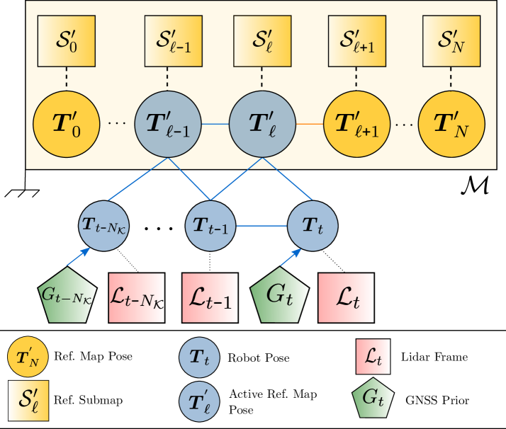
Figure 1: Overview of the proposed graph-based localization method using prior topological and metric information from the environment. Blue elements form the active graph and orange elements the reference graph.

At first glance, without the need of updating an environment model, the use of Global Navigation Satellite System (GNSS) in (semi-)urban areas may seem convenient for localization, although its use alone has long been proven to be neither robust nor accurate enough for the required applications [6]. Combining measurements from multiple sensors and finding correspondences with a reference map model is key to robust, reliable and accurate localization in automotive applications. Most of the existing work tackles this task by using filters for measurement integration, and by exploiting dense high-resolution point cloud maps previously generated by SLAM algorithms [7, 8, 9]. However, modern SLAM systems, based on probability and graph theories [1], contain much more information beyond the resulting reconstruction: a rich underlying graph that captures the localization estimates and accommodates the observation uncertainties. This valuable topological information has been overlooked in the literature.

In this work, we present G-Loc, a novel tightly-coupled graph localization approach that exploits prior topo-metric knowledge of the environment. We associate this information with LiDAR (Light Detection And Ranging) measurements and seamlessly integrate it with IMU (Inertial Measurement Unit) and GNSS data in a robust and efficient manner. We aim to encourage the use of all available information generated by modern SLAM systems,going beyond purely metric maps.

The rest of the paper is organized as follows. Section II discusses related work and the contributions of this paper, Section III formally defines the problem, Section IV details the components of our system, and Section V contains the experimental results. This letter is concluded in Section VI.

II Related Work

Levinson et al. [6] are among the first to exploit a previously-built map for localization. They correlate LiDAR intensity measurements with the prior map (a grid representation containing a Gaussian distribution of intensity in each cell) using a particle filter. They also incorporate GNSS measurements to limit particle dispersion. However, this and other related work [10, 11], reduce the estimation problem to 3 degrees of freedom, assuming that the rest are estimated, e.g., from an IMU. [12] estimates a global 3D pose instead after incorporating altitude into the distribution of the cells.

A different approach is followed in [13], where the reference map consists of road primitives. An unscented Kalman filter is used to combine GNSS, odometry and the matching between the prior map and the online primitives extracted from images via convolutional neural networks. The challenge of maintaining and matching a dense point cloud map is also addressed in [14], where such representations are transformed into a sparse multi-layer vector map, and [15], where features are extracted from lateral galleries in a tunnel-like environment.

More recently, advances in point cloud registration have brought these methods to the forefront of map-based localization, whether feature-based or not. Yoneda and Mita [7] first matched LiDAR measurements to a geo-referenced point cloud map using Iterative Closest Point (ICP) [16]. The limitations of this single sensor approach and the sensitivity of ICP to the initial guess are addressed in subsequent works, all of them being filter-based [8, 17, 9, 18, 19, 20]. Nagy and Benedek [9] fuse point cloud and semantic matching with GNSS measurements to localize a robot in a high resolution 3D semantic cloud. In [21], instead of matching the online LiDAR data to the reference point cloud map, the latter is rendered in 2D; this allows to match monocular images. Autoware [8], a widely used open-source library constantly under development, features global localization in a prior map (either in the form of a point cloud or a high-definition vector map). This approach relies on aligning the input clouds with the reference map using the Normal Distribution Transform (NDT) [22] technique. The optimized transformation is integrated with IMU and GNSS measurements within an extended Kalman filter module. PoseMap [23] incorporates the trajectory into the prior model, thus going beyond purely metric representations. Each of the robot poses is assigned a submap of surfels and the alignment of the online cloud is done only with the $k$-closest neighbors, significantly reducing the computational cost and allowing to take advantage of the full LiDAR range.

In contrast to the filter-based techniques mentioned above, a handful of methods have recently started to use a graph formulation, borrowing from the advances in graph SLAM and due to its improved robustness and accuracy [24]. Dubé et al. [25] estimate the robot’s pose in a prior global map by extracting segments from a 3D point cloud and matching neighbors in the feature space. The resulting transformations are later fed into a pose-graph SLAM framework along with pre-integrated IMU measurements. [26] also employs a pose-graph formulation for localization, combining wheel odometry, GNSS, and semantic matching with the reference map.

In parallel to our work, Koide et al. [27] recently proposed a map-based localization approach that tightly couples range and IMU data within a sliding window factor graph optimization.

The localization method proposed in this letter falls into the graph-based category. In contrast to previous work, we combine GNSS data, IMU pre-integrated measurements, LiDAR odometry and map-matching constraints within a graph optimization framework, thus achieving global localization in a robust and efficient manner. Furthermore, we go beyond dense metric representations (unlike [25, 26, 27]) and fully exploit the prior knowledge obtained during the mapping task, somewhat following [23] but leveraging the pose-graph topology instead of just the trajectory poses. This allows us not only to relax the neighborhood search and restrict the alignment of the online clouds to certain regions of the reference map (i.e., submaps), but also to integrate those neighboring reference nodes into the optimization framework (see Figure 1). G-Loc is a modular and optimized framework that adapts to a wide variety of algorithms and sensors with minimal parameter tuning and is capable of handling large-scale environments. We have validated the proposed method on several datasets, as well as in a real automotive application, demonstrating the robustness and accuracy of G-Loc even in map-less regions compared to other popular state-of-the-art methods.

III Problem Formulation

Map-based localization aims to determine the pose of a robot or sensor within an existing map of the environment. This can intuitively be seen as a coordinate transformation process, which consists of establishing correspondences between the map information and the current perception [28].

First of all, let us denote the map and robot base frames by $m$ and $r$, respectively. To simplify the notation, all the sensors will be assumed to be in $r$. In its most basic form, map-based 3D localization can be formulated as the problem of estimating the robot poses that best match the sensor observations with each other and with the map, i.e., finding the maximum a posteriori (MAP) estimates

$$\mathcal{T}^{\star}\triangleq\underset{\mathcal{T}}{\mathrm{argmax}}\ p(\mathcal{T}\,|\,\mathcal{M},\mathcal{Z})\,,$$ (1)

where $p(\cdot)$ denotes probability, $\mathcal{M}$ is the prior map, $\mathcal{Z}$ is the set of sensor measurements, and $\mathcal{T}\triangleq\{\boldsymbol{}^{m}{T}_{r_{i}}\in SE(3)\,|\,i\in\mathcal{K}_{t}\}$ is the set of relative transformations between the map and the latest $N_{\mathcal{K}}\texttt{+}1$ robot frames. To maintain tractability, the set of frames $\mathcal{K}_{t}\triangleq\{\max(0,t\texttt{-}N_{\mathcal{K}}),\dots,t\}$ has been limited in a sliding window fashion.

On the one hand, we assume that $\mathcal{M}$ has been previously built by a graph-SLAM algorithm, and thus contains metric and topological information (in the form of point clouds and a pose-graph, respectively). Furthermore, the metric part is associated with the nodes of the graph in such a way that each vertex is assigned a set of point clouds (or submap, $\mathcal{S}$) of its surroundings (see upper part of Figure 1). Then:

$$\mathcal{M}\triangleq\left\{\mathcal{G}\,,\mathcal{S}_{\ell}\,|\,\ell\in\mathcal{R}\right\}\,,$$ (2a)

$$\mathcal{G}\triangleq\{\mathcal{V},\mathcal{E}\}\,,$$ (2b)

$$\mathcal{S}_{\ell}\triangleq\{\mathcal{L}_{q}^{\ell}\,|\,q=1,\dots,N_{\mathcal{S}_{\ell}}\}\,,$$ (2c)

where $\mathcal{R}\triangleq\{0,\dots,\dim(\mathcal{V})\}$ is the reference frame set, $(\mathcal{V},\mathcal{E})$ are the sets of vertices and edges in the pose-graph $\mathcal{G}$, and any given point cloud $\mathcal{L}\triangleq\{\tilde{\boldsymbol{p}}_{l}\in\mathbb{R}^{3}\,|\,l\,\texttt{=}\,1,\dots,N_{\mathcal{L}}\}$. Notice that the submaps of nearby vertices might overlap and that elements of the pose-graph will live in $SE(3)$. Additionally, the graph may contain GNSS information, making also the map geo-referenced and aligned to the East, North, Up (ENU) global coordinate system.

On the other hand, the set of measurements collected up to time $t$ consists of LiDAR point clouds, IMU observations between consecutive frames, and GNSS data:

$$\mathcal{Z}_{t}\triangleq\{\mathcal{Z}^{\text{LiDAR}}_{i},\mathcal{Z}^{\text{IMU}}_{i,j},\mathcal{Z}^{\text{GNSS}}_{i}\}_{i,j\in\mathcal{K}_{t}}\,.$$ (3)

Assuming (i) that the robot poses are normally distributed (i.e., $\boldsymbol{T}\triangleq\boldsymbol{\bar{T}}\exp(\boldsymbol{\delta})\in SE(3)$, with $\boldsymbol{\bar{T}}$ a large mean transformation and $\boldsymbol{\delta}\in\mathbb{R}^{6}$ a random vector normally distributed around zero) and pairwise independent, (ii) the measurements are conditionally independent w.r.t. the poses, and (iii) LiDAR and IMU observations are combined to provide odometry estimates, (1) can be rewritten as follows:

$$\mathcal{T}^{\star}=\underset{\mathcal{T}}{\mathrm{argmin}}\ \boldsymbol{F}(\mathcal{T})$$ (4)

$$\text{s.t.}\ \boldsymbol{F}(\mathcal{T})=\sum\limits_{i,j\in\mathcal{K}_{t}}\|\boldsymbol{e}_{i,j}^{\text{LIO}}\|^{2}+\sum\limits_{i\in\mathcal{K}_{t}}\|\boldsymbol{e}_{i}^{\mathcal{M}}\|^{2}+\sum\limits_{i\in\mathcal{K}_{t}}\|\boldsymbol{e}_{i}^{\text{GNSS}}\|^{2}\,,$$

where $\|\boldsymbol{e}\|^{2}\triangleq(\boldsymbol{e}^{T}\boldsymbol{\Sigma}^{\texttt{-}1}\boldsymbol{e})\in\mathbb{R}$ is the quadratic error for a measurement with covariance $\boldsymbol{\Sigma}$. $\boldsymbol{e}_{i,j}^{\text{LIO}}$ are the residual errors associated with the LiDAR-inertial odometry (LIO) estimates (described in Section IV-A), $\boldsymbol{e}_{i}^{\mathcal{M}}$ are those associated with the correspondences between LiDAR observations and the prior map (Section IV-B), and $\boldsymbol{e}_{i}^{\text{GNSS}}$ are the translation errors associated with the GNSS measurements.

IV Methods

G-Loc is divided into three main threads, namely: LIO, Localization and Dynamic Loading, to which the following subsections are dedicated. Figure 2 contains an overview of the system, illustrating the different modules and their connections. Thanks to its parallelized architecture, the entire system runs in real time within a ROS2 Humble [29] framework. It is able to use GPU-accelerated cloud registration methods, and it is robust to a wide variety of sensor configurations with minimal parameter tuning.

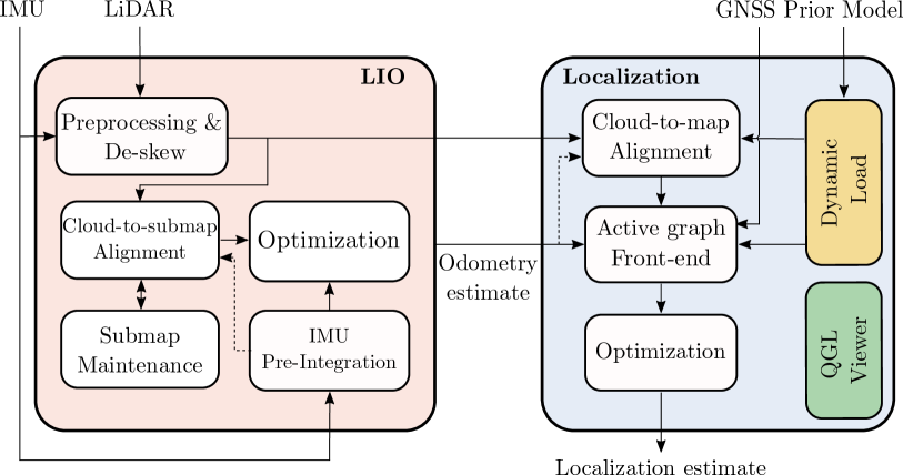
Figure 2: Block diagram of G-Loc. The dashed lines represent the initial guess fed to the registration methods.

LIO combines range and inertial measurements within a graph optimization framework. Online LiDAR data is aligned with most recent point clouds (which are contained in a submap), and high-frequency IMU data is pre-integrated for an efficient optimization. The output of LIO is then fed into the localization module, along with GNSS measurements and the results from cloud-to-map registration. A second pose-graph is optimized taking into account the previous constraints. Splitting the optimization problem into two different graphs improves the stability and convergence of the system and facilitates the noise configuration [30]. The dynamic loader allows to work with large prior maps by limiting the number of point clouds loaded in memory. Finally, visualization is based on OpenGL and handled in a separate thread.

IV-A LiDAR-inertial Odometry (LIO)

Relative measurements between consecutive robot poses are computed in a graph-based LIO framework. The incremental inertial state can be defined as

$$\mathcal{X}\triangleq\{\boldsymbol{x}_{i}\,|\,i\in\mathcal{I}_{t}\}\,,$$ (5a)

$$\boldsymbol{x}_{i}\triangleq\{\boldsymbol{T}_{i},\ \boldsymbol{v}_{i},\ \boldsymbol{b}_{i}\}\,,$$ (5b)

where $\boldsymbol{v}\in\mathbb{R}^{3}$ is the linear velocity and $\boldsymbol{b}=(\boldsymbol{b}^{g},\boldsymbol{b}^{a})\in\mathbb{R}^{6}$, with $\boldsymbol{b}^{g}$, $\boldsymbol{b}^{a}$ in $\mathbb{R}^{3}$ the gyroscope and accelerometer bias, respectively. The dimension of $\mathcal{X}$ is constrained by $\mathcal{I}_{t}\triangleq\{\max(0,t\texttt{-}N_{\mathcal{I}}),\dots,t\}$, similarly to $\mathcal{K}_{t}$. The map frame superindex notation has been dropped for readability.

First, a preprocessing step is performed. The input cloud is downsampled to a desired voxel resolution, and points too close/distant are removed. Then, a de-skew operation is performed to mitigate the noise in the input scan $\mathcal{L}_{t}$. In this way, the angular distortion caused by the robot’s ego-motion while capturing the data is corrected. Since each point has an associated acquisition timestamp, angular velocity measurements from the IMU can be integrated and then interpolated to compute the relative orientation w.r.t. the start of the scan.

The de-skewed cloud is then aligned with the previous submap $\mathcal{S}_{t-1}$ created by concatenating the $N_{\mathcal{S}}$ previous point clouds (see Figure 3). Scan-to-submap alignment relies either on ICP or NDT techniques. Our system supports a variety of registration methods, but two have proven to be superior: (i) the efficient and GPU-accelerated implementation of voxelized generalized ICP [31], and (ii) the parallelized version of NDT. This process outputs LiDAR odometry (LO) estimates between frames (i.e., the transformations ${}^{i\texttt{-}1}\tilde{\boldsymbol{T}}^{\text{LO}}_{i}$), which can be introduced into the graph as prior edges to constrain the pose of the inertial state after computing ${}^{i}\tilde{\boldsymbol{T}}^{\text{LO}}=\left(\boldsymbol{T}_{i\texttt{-}1}\ {}^{i\texttt{-}1}\tilde{\boldsymbol{T}}^{\text{LO}}_{i}\right)^{\texttt{-}1}$. The residuals for the $i$-th frame will be given by:

$$\boldsymbol{e}_{i}^{\text{LO}}\triangleq\log\left(\boldsymbol{T}_{i}\ {}^{i}\tilde{\boldsymbol{T}}^{\text{LO}}\right)^{\vee}\in\mathbb{R}^{6}\,,$$ (6)

where the logarithm and vee operators are, respectively, $\log(\cdot):SE(3)\mapsto\mathfrak{se}(3)$ and $(\cdot)^{\vee}:\mathfrak{se}(3)\mapsto\mathbb{R}^{6}$, being $\mathfrak{se}(3)$ the Lie algebra of $SE(3)$. The covariance of this measurement is inherited from the registration method [31]. Note that only unaccented variables will be optimization variables.

Simultaneously with the above, IMU measurements between LiDAR frames are pre-integrated following [32]. Pre-integration provides an estimate of the robot’s motion between successive frames, also allowing the scan-to-submap matching to be fed with a decent initial guess (see Figure 3). IMU data is efficiently incorporated into the graph optimization framework by creating an inertial edge [30, 2] between frames; this edge is actually composed of several different edges that correlate the poses and velocities between frames, and also model the bias variation over time (assumed to follow a Brownian motion pattern). Acceleration and rotation rate measurements ($\tilde{\boldsymbol{a}}$ and $\tilde{\boldsymbol{\omega}}$) can be integrated between $i$-th and $j$-th LiDAR frames to estimate the evolution of the sensor’s pose and velocity. Let us consider the motion model:

$$\boldsymbol{R}_{j} =\boldsymbol{R}_{i}\textstyle\prod\limits_{k=i}^{j-1}\exp((\tilde{\boldsymbol{\omega}}_{k}\texttt{-}\boldsymbol{b}_{k}^{g}\texttt{-}\boldsymbol{\eta}_{k}^{g})\Delta t)\,,$$

$$\boldsymbol{v}_{j} =\boldsymbol{v}_{i}+\boldsymbol{g}\Delta t+\textstyle\sum\limits_{k=1}^{j-1}\boldsymbol{R}_{k}(\tilde{\boldsymbol{a}}_{k}\texttt{-}\boldsymbol{b}_{k}^{a}\texttt{-}\boldsymbol{\eta}_{k}^{a})\Delta t\,,$$

$$\boldsymbol{p}_{j} =\boldsymbol{p}_{i}+\textstyle\sum\limits_{k=1}^{j-1}\left(\boldsymbol{v}_{k}\Delta t+\frac{1}{2}\boldsymbol{g}\Delta t^{2}+\frac{1}{2}\boldsymbol{R}_{k}(\tilde{\boldsymbol{a}}_{k}\texttt{-}\boldsymbol{b}_{k}^{a}\texttt{-}\boldsymbol{\eta}_{k}^{a})\Delta t^{2}\right)\,,$$ (7)

with $\Delta t$ the time between the two frames, $\boldsymbol{\eta}^{g},\boldsymbol{\eta}^{a}\in\mathbb{R}^{3}$ additive white noise and $\boldsymbol{T}\triangleq(\boldsymbol{R},\boldsymbol{p})$, where $\boldsymbol{R}\in SO(3)$ and $\boldsymbol{p}\in\mathbb{R}^{3}$. From (7), we can define the relative increments between frames and the preintegrated measurement model, i.e., $\Delta\tilde{\boldsymbol{R}}_{ij}$, $\Delta\tilde{\boldsymbol{v}}_{ij}$ and $\Delta\tilde{\boldsymbol{p}}_{ij}$ (see [32] for details). Using them, the residual error of the IMU measurements $\boldsymbol{e}^{\text{IMU}}\triangleq(\boldsymbol{e}_{\Delta\boldsymbol{R}},\boldsymbol{e}_{\Delta\boldsymbol{v}},\boldsymbol{e}_{\Delta\boldsymbol{p}},\boldsymbol{e}_{\Delta\boldsymbol{b}})^{T}\in\mathbb{R}^{15}$ will be given by [32]:

$$\boldsymbol{e}_{\Delta\boldsymbol{R}_{i,j}} \triangleq\log(\Delta\tilde{\boldsymbol{R}}_{ij}^{T}\boldsymbol{R}_{i}^{T}\boldsymbol{R}_{j})^{\vee}\,,$$ (8a)

$$\boldsymbol{e}_{\Delta\boldsymbol{v}_{i,j}} \triangleq\boldsymbol{R}_{i}^{T}(\boldsymbol{v}_{j}\texttt{-}\boldsymbol{v}_{i}\texttt{-}\boldsymbol{g}\Delta t_{i,j})\texttt{-}\Delta\tilde{\boldsymbol{v}}_{ij}\,,$$ (8b)

$$\boldsymbol{e}_{\Delta\boldsymbol{p}_{i,j}} \triangleq\boldsymbol{R}_{i}^{T}(\boldsymbol{p}_{j}\texttt{-}\boldsymbol{p}_{i}\texttt{-}\boldsymbol{v}_{i}\Delta t_{i,j}\texttt{-}\frac{1}{2}\boldsymbol{g}\Delta t_{i,j}^{2})\texttt{-}\Delta\tilde{\boldsymbol{p}}_{ij}\,,$$ (8c)

all of which live in $\mathbb{R}^{3}$, and $\boldsymbol{e}_{\Delta\boldsymbol{b}_{i,j}}\triangleq\boldsymbol{b}_{j}-\boldsymbol{b}_{i}\in\mathbb{R}^{6}$. Note that the vee and logarithmic operators are now over $SO(3)$.

Finally, the graph containing the above constraints (see Figure 3) is optimized using g2o [33], solving the optimization:

$$\mathcal{X}^{\star}=\underset{\mathcal{X}}{\mathrm{argmin}}\left(\sum_{i\in\mathcal{I}_{t}}\|\boldsymbol{e}_{i}^{\text{LO}}\|^{2}+\sum_{i,j\in\mathcal{I}_{t}}\|\boldsymbol{e}_{i,j}^{\text{IMU}}\|^{2}\right)$$ (9)

High-frequency odometry (at IMU rate) can be obtained by composing the LO with the relative motion predictions from the preintegrated measurement model.

The success of any registration algorithm depends on a good initial guess and sufficient overlap between the input clouds. The first issue has already been addressed, and the second is mitigated by the submaps, which in turn require some maintenance. After adding a new point cloud to the submap, it is voxelized (e.g., via uniform sampling) to prune redundant points. To restrain complexity, the submap size is limited to include the last $N_{\mathcal{S}}$ point clouds. A side effect of this approach is high adaptability to different range sensors: we can handle densities from 16 to 128 beams and different patterns by changing $N_{\mathcal{S}}$ (e.g., submaps containing one single cloud are suitable for 128-plane LiDARs). This provides the flexibility to work with different sensors with minimal parameter tuning. By effectively configuring the submaps, we can also keep the computational cost within reasonable limits for the resources available and the precision required in each application.

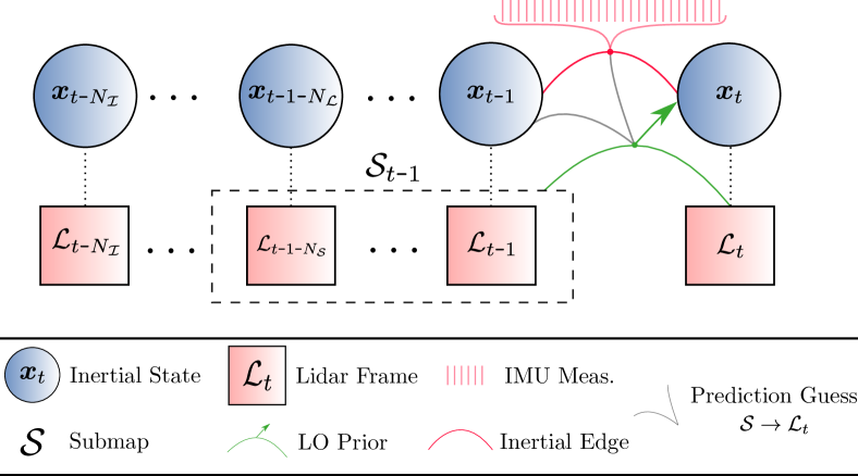
Figure 3: Scheme of how the different constraints are integrated into the graph-based LIO optimization framework.

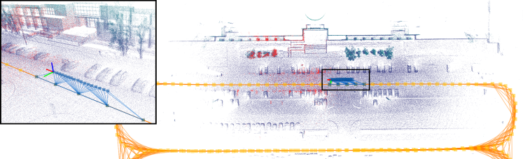
Figure 4: Visualization of G-Loc. The prior graph is shown in orange and the active graph in blue (vertices are represented as squares and edges as lines connecting them). The upper left corner displays a zoom of the active graph, which consists of the sliding graph and a subgraph of the prior model. The online LiDAR cloud is shown as red points, while the loaded submaps of the prior model are colored by height. Note that only a subset of the metric model (i.e., the submaps corresponding to vertices within the robot’s neighborhood) has been loaded.

IV-B 3D Graph-based Localization

The main (global) localization process is based on optimizing a sliding graph together with regions of interest of the reference graph (see Figure 1).

The localization process starts with estimating the robot’s initial pose within the prior map using GNSS measurements. It then queries the prior topo-metric model to find the $k$-closest reference vertices (for the exemplary graph shown in Figure 1, at time $t$, it will be $\boldsymbol{T}^{\prime}_{\ell}$). Next, the current 3D LiDAR scan is aligned with the submaps associated with these vertices ($\mathcal{S}_{\ell}^{\prime}$). The active graph combines the constraints enforced by the results of these alignments along with the relative motion data provided by the LIO module and GNSS measurements (if available). Therefore, this new graph will contain vertices from both the prior reference graph and the online sliding graph; the latter encodes current and past robot states in a sliding window approach (i.e., $\mathcal{T}$). The size of the sliding graph is limited to $\dim(\mathcal{T})$), being older nodes marginalized as they leave the window. Figure 4 displays the active (blue) and reference (orange) graphs on top of the prior point cloud map for an example localization task. The online cloud is shown in red. As shown in the zoomed area, multiple reference vertices can be associated with a single vertex in the sliding graph.

The optimization of the active graph is governed by (4), subject to:

$$\boldsymbol{e}_{i,j}^{\text{LIO}} \triangleq\log\left(\boldsymbol{T}_{i}\ {}^{i}\tilde{\boldsymbol{T}}^{\text{LIO}}_{j}\ (\boldsymbol{T}_{j})^{\texttt{-}1}\right)^{\vee}\in\mathbb{R}^{6}\,,$$ (10a)

$$\boldsymbol{e}_{i}^{\mathcal{M}} \triangleq\sum\limits_{k\in\mathcal{R}_{i}}\log\left(\boldsymbol{T}_{i}\ {}^{i}\tilde{\boldsymbol{T}}_{k}^{\mathcal{M}}\ (\boldsymbol{T}^{\prime}_{k})^{\texttt{-}1}\right)^{\vee}\in\mathbb{R}^{6}\,,$$ (10b)

$$\boldsymbol{e}_{i}^{\text{GNSS}} \triangleq\boldsymbol{p}_{i}\texttt{-}\tilde{\boldsymbol{p}}_{i}\in\mathbb{R}^{3}\,,$$ (10c)

where ${}^{i}\tilde{\boldsymbol{T}}^{\text{LIO}}_{j}$ is the output from the previous subsection, ${}^{i}\tilde{\boldsymbol{T}}_{k}^{\mathcal{M}}$ are the registration results between the current scan and the prior map, and $\boldsymbol{T}^{\prime}_{k}\in\mathcal{G}$. Note that correspondences with the prior map are only evaluated for a subset of the reference frames, i.e., $k\in\mathcal{R}_{i}\subset\mathcal{R}$. Finally, $\tilde{\boldsymbol{p}}_{i}={}^{\text{UTM}}\tilde{\boldsymbol{p}}_{i}\texttt{-}{}^{\text{UTM}}\tilde{\boldsymbol{p}}_{m}$, with ${}^{\text{UTM}}\tilde{\boldsymbol{p}}_{i}$ the actual GNSS measurement and ${}^{\text{UTM}}\tilde{\boldsymbol{p}}_{m}$ the origin of the prior model (i.e., the GNSS estimation for the first vertex). Note that this origin will be associated with a UTM (Universal Transverse Mercator) coordinate. Relativizing GNSS allows to merge it with cloud-to-map matching and LIO constraints.

Dataset	Length	$\Delta$ Elevation	LiDAR	IMU	GNSS
EU long-term (ref. & eval.)	$\sim 5\phantom{.0}$ km	$\sim 50$ m	2x Velodyne HDL-32E	XSens MTi-28A53G25	Magellan ProFlex 500
UZ Campus (ref.)	$\sim 2.7$ km	$\sim\phantom{0}1$ m	Ouster OS1-128		Ardusimple RTK2B
UZ Campus (eval.)	$\sim 1.5$ km	$\sim\phantom{0}1$ m	Livox HAP
Bus	$\sim 8\phantom{.0}$ km	$\sim 70$ m	2x RS Helios 32-5515	XSens MTI-680-G

TABLE I: Summary of the sensor configurations and environmental characteristics in the experiments performed.

On the one hand, LIO relative measurements are used to connect sequential vertices of the sliding graph with information depending on the alignment result (defined as the mean error between all matched points, weighted by the match percentage). In addition, it also provides an initial guess for the cloud-to-map registration. On the other hand, registrations between the current scan and the reference submaps are introduced as binary edges between vertices in the reference and sliding graphs, with information also depending on the alignment result. Also, the transformation with the highest information is used to compute the initial estimate for the optimization process (also handled by g2o). The previous constraints connect the two graphs and form the active graph (blue elements in Figure 1). Should the sliding and reference graphs become disconnected, either due to alignment failure or the lack of nearby reference vertices, the algorithm will rely on LIO and GNSS until re-localization occurs. Finally, GNSS measurements are used as prior unary edges (blue arrows in Figure 1). These constraints are only incorporated if they are synchronized with the online cloud and if their uncertainty is below a certain threshold, thus rejecting noisy measurements.

IV-C Dynamic Loading

A dynamic loader is used to relax the high memory requirements of loading large point cloud maps. This module allows loading only nearby parts of the reference model, $\mathcal{M}$, as the robot moves; this is especially useful for large maps where maintaining (and visualizing) all submaps at high resolution is intractable. Since both the reference and sliding graphs are geo-referenced, it is possible to load the submaps near the current robot localization estimate in a sliding window fashion. To do this, we query the nearby vertices in the reference graph (i.e., within a specified Euclidean distance) and keep only their associated submaps in memory. In Figure 4, only the submaps that are close to the active graph (shown in blue) are loaded into memory and thus visualized in a large environment.

V Experimental Results

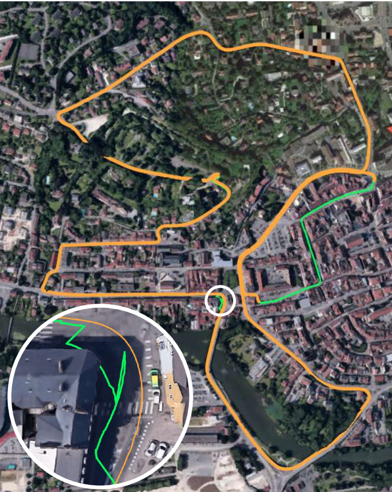
((a))

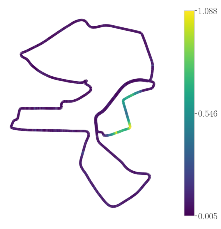
((b))

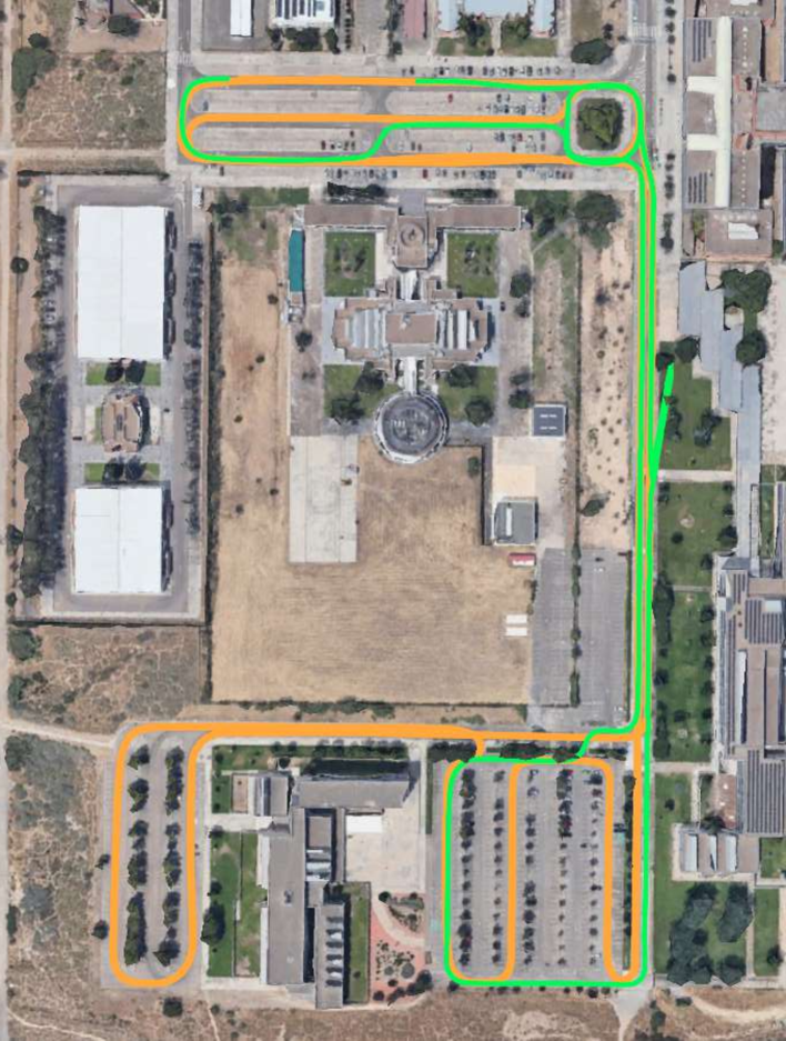
((c))

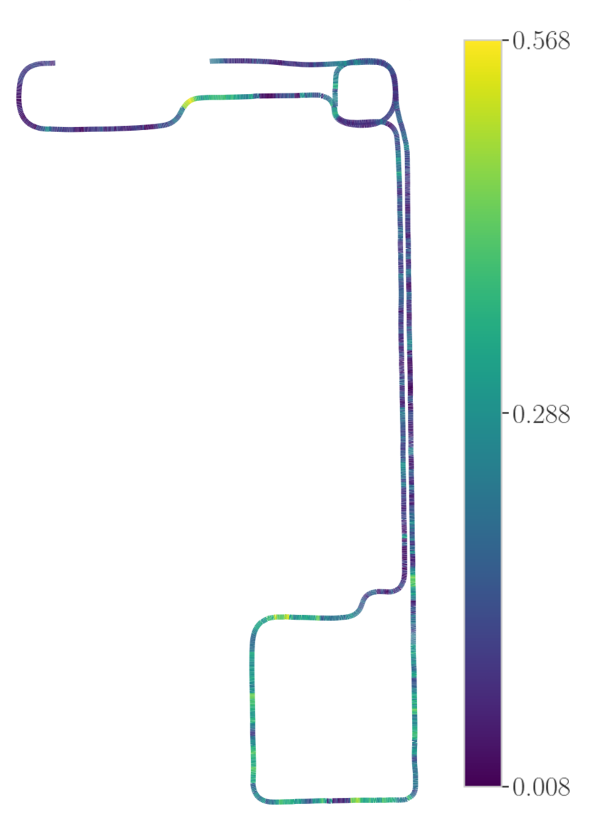
((d))

Figure 5: Evaluation results in the EULT (a)-(b) and UZ Campus (c)-(d) datasets. (a), (c): geo-referenced SLAM trajectories in the reference sequences (orange) and raw GNSS data in the evaluation sequences (green). (b), (d): Trajectories estimated by G-Loc in the evaluation sequences; the color map indicates 2D ATE (darker is smaller).

In this section, we present a thorough evaluation of G-Loc in different applications and under different sensor configurations, demonstrating the versatility of our approach. We use two real urban datasets: EU long-term dataset [34] and our own dataset collected on the campus of the University of Zaragoza (UZ). In addition, we present the results of using G-Loc in a real-world automotive application, in the context of an autonomous driving bus. The dataset experiments were performed on a laptop equipped with an Intel Core i7 CPU (8 cores) and an Nvidia GeForce RTX 3080 GPU, while the bus was equipped with an Intel Core i9 CPU (24 cores) and a Nvidia A2000 GPU (note that many other processes for autonomous driving were running concurrently on this hardware). Unless otherwise noted, [31] was used for registration. Table I contains a short summary of the experiments and the sensors installed in the mobile platforms. The results presented in this section were obtained using evo.

V-A Dataset Evaluation

The EU long-term dataset contains several sequences recorded with a car in a downtown. They all follow a similar trajectory under different conditions (e.g., traffic, weather); this is particularly interesting for testing localization, since we need different but overlapping reference and evaluation trajectories. The length of each sequence is about $5$ km with a duration of $16$ minutes. The sensor configuration is detailed in Table I.

To evaluate the performance of G-Loc on this dataset, we first generated a geo-referenced model of the environment using one of the available sequences, which will be referred to as reference sequence. We used a SLAM system that inherits the architecture shown in Figure 2 but replaces the localization module with a mapping module that features robust loop closing and global optimization. This way, we obtained the required prior model with topological (a pose-graph) and metric (point cloud submaps) information. To evaluate the performance in map-less regions, we removed an entire road from the prior model (approximately $0.4$ km); the SLAM-estimated trajectory is shown in orange in Figure 5(a). The built model was fed into G-Loc while running two different evaluation sequences4. Figure 5(a) also shows the raw GNSS data (green) for one of the evaluation sequences to facilitate its comparison with the reference trajectory; the middle right part contains the cropped region, where there is GNSS signal but no prior information. Whenever the robot traverses a mapped region, the prior model is exploited to improve localization and correct for potential drift in LIO. In unmapped regions, the sliding graph disconnects from the reference graph, accumulating larger errors that are eventually corrected after re-localization. Figure 5(b) contains the 2D Absolute Trajectory Error (ATE) for translation (in meters) along the trajectory for one of the sequences, clearly showing that the highest errors occur on the unmapped road and that even under these conditions they are within reasonable limits. Table II contains the numerical results (mean and standard deviation) for this experiment, namely 3D ATE for translation and rotation, and lateral and longitudinal error. This table also reports the results of using a complete prior map (i.e., without cropping a road); in this case, the errors were similar but show a smaller deviation. We evaluated the use of parallelized NDT, which runs entirely on the CPU and is of particular interest for resource-constrained platforms. In this case, localization errors were slightly higher than with GPU acceleration.

Finally, to benchmark G-Loc, we conducted the same experiments using Autoware localization module [8], which represents a popular state-of-the-art localization system for autonomous vehicles. It is based on an extended Kalman filter that integrates velocity measurements with cloud-to-map alignments and a GNSS regularization term. For a fair comparison, we fed velocity measurements from our LIO module and used parallelized NDT for registration. Autoware failed to localize in the mapless region, leading to an unrecoverable state. Using the complete prior model, the translation errors were comparable to G-Loc but the rotational error was nearly doubled (see Table II). In addition, Autoware required using an Intel Core i9 CPU with 24 cores to work properly.

Dataset	Method	ATE (trans., m)	Long. Error (m)	Lat. Error (m)	ATE (rot., deg)	Time per frame (ms)
EULT (cropped)	G-Loc (GPU)	0.209 (0.395)	0.087 (0.280)	0.048 (0.228)	0.423 (0.445)	25.13 (7.82)
	G-Loc (CPU)	0.240 (0.300)	0.086 (0.304)	0.021 (0.208)	1.008 (1.160)	38.01 (14.86)
	Autoware	$\phantom{{}^{\dagger}}-$	$\phantom{{}^{\dagger}}-$	$\phantom{{}^{\dagger}}-$	$\phantom{{}^{\dagger}}-$	$\phantom{{}^{\ddagger}}-$
EULT (complete)	G-Loc (GPU)	0.194 (0.201)	0.101 (0.240)	0.014 (0.197)	0.440 (0.576)	26.47 (4.31)
	G-Loc (CPU)	0.218 (0.196)	0.119 (0.245)	0.009 (0.203)	0.953 (0.836)	40.13 (12.99)
	Autoware	0.212 (0.194)	0.123 (0.232)	0.006 (0.203)	0.784 (1.380)	‡37.31 (14.52)
UZ Campus	G-Loc (GPU)	0.154 (0.102)	0.071 (0.132)	0.019 (0.126)	0.473 (0.537)	34.62 (9.14)
	G-Loc (CPU)	0.214 (0.151)	0.131 (0.179)	0.014 (0.158)	0.650 (0.878)	72.15 (31.54)
	Autoware	†0.308 (1.251)	†0.400 (0.655)	†0.086 (1.353)	†2.146 (0.850)	‡59.74 (71.47)

TABLE II: Localization errors (mean and std. dev.) and time consumed per frame for G-Loc (GPU and CPU) and Autoware in the evaluated datasets. ($-$) indicates an unrecoverable failure in localization. The best results for each dataset are shown in bold.

The UZ Campus dataset was captured using a sensor-equipped car. We recorded two sequences, which partially overlap, but with two different LiDAR sensors. See Table I.

To evaluate this dataset, we followed a similar procedure as before. First, we built the prior model with a reference sequence using a high-performance sensor with $360\degree$ Field of View (FoV) and $128$ planes. Then, we evaluated G-Loc with an evaluation sequence, exploiting the prior topo-metric knowledge and using a LiDAR with $120\degree$ FoV and a completely different sensing pattern. Figure 5(c) displays the trajectory of the reference sequence (orange) and the raw GNSS data for the evaluation one (green). Both trajectories overlap for most of the route, and when they do not, they are close enough so that the prior map can be used (unlike in EULT). ATE error along the trajectory is shown in Figure 5(d) and numerical results are reported in the bottom of Table II. As in EULT, the use of the GPU gave the best results, except for the lateral error (however, these lower mean values are accompanied by higher variance). This experiment demonstrates the adaptability of our method to the use of different sensors for building the prior map and localization. The submaps played a fundamental role here, mitigating the effects of the different sensing patterns and feeding the registration algorithms with sufficient overlapping regions. In contrast, Autoware accumulated much higher errors and had difficulty finding correspondences in many regions (which explains the large deviations), eventually leading to an unrecoverable state. The results reported in Table II for this experiment (marked with ^†) are only before this divergence.

V-B On the Time Consumption

While the above section aimed to demonstrate the robustness and precision of our approach, we now seek to demonstrate its real-time performance. The processing times per frame consumed by each algorithm in the conducted experiments are listed in Table II. G-Loc required, on average, $25$ ms in EULT and $34$ ms UZ Campus —this is much faster than the typical LiDAR frame rate ($10$ Hz) and therefore meets real-time requirements. In both cases, LIO accounts for $60\%$ of that time, and the localization module for the rest (visualization and dynamic load are excluded as they operate in the background). The fact that two different sensors were used in the second dataset resulted in longer registration times. G-Loc without GPU took considerably longer, but the frame rate was generally not exceeded. We also report the results for Autoware (marked with ^‡), which are similar to G-Loc without GPU. Note, however, that Autoware used a more powerful CPU and had 3 times the number of cores available to parallelize computations, so the direct comparison is unfair.

Finally, we compared the use of G-Loc to naively running a full SLAM system again to reveal the time benefits of exploiting the known prior topo-metric map instead of using a new map. We ran this experiment on the EULT dataset because it is the largest and therefore where a new map would be more costly to generate and maintain. At first glance, the time required to process each frame might seem similar to that of G-Loc (the LIO update), but the graph optimization and loop closing threads took $90.4\pm 101.4$ ms (this scales with the graph size, unlike in G-Loc that optimizes a bounded-sized sliding graph) and $100.2\pm 0.4$ ms, respectively. These demanding processes usually slowed down the entire pipeline and caused interruptions in the localization estimates.

V-C Real-world Deployment

G-Loc has been deployed on an autonomous bus (see Figure 6(a)) on an urban bus line in the city of Zaragoza (Aragón, Spain) as part of the pioneering Spanish project on urban driving, DIGIZITY. The sensors installed on the vehicle and the route specifics appear in Table I. Our system requires coordination with other navigation systems to provide a robust and reliable localization, ensuring safe navigation even in areas with poor GNSS coverage due to large buildings; accurate localization is critical as the bus must autonomously stop at designated bus stops and obey traffic lights. The prior model of the entire route ($\sim 8$ km) is shown in Figure 6(b). In addition, localization starts as soon as the bus is turned on. This means that the localization has to work without a prior model from the departure point until the route is reached ($\sim 2$ km). The system localizes in the unmapped region using LIO and GNSS in a sliding-graph optimization fashion until re-localization with the prior model occurs. Figure 6(c) depicts the trajectory estimated by G-Loc for a single trip, and Figure 6(d) shows the improvement of these estimates (blue) over the raw GNSS data (green) in one of the many low coverage areas. During the deployment, the bus operated seamlessly for about $100$ hours over a span of $20$ days, covering about $800$ km. Notably, there were no localization failures and the errors remained within bounds comparable to previous results (i.e., at the cm level), further showcasing the robustness and accuracy of G-Loc.

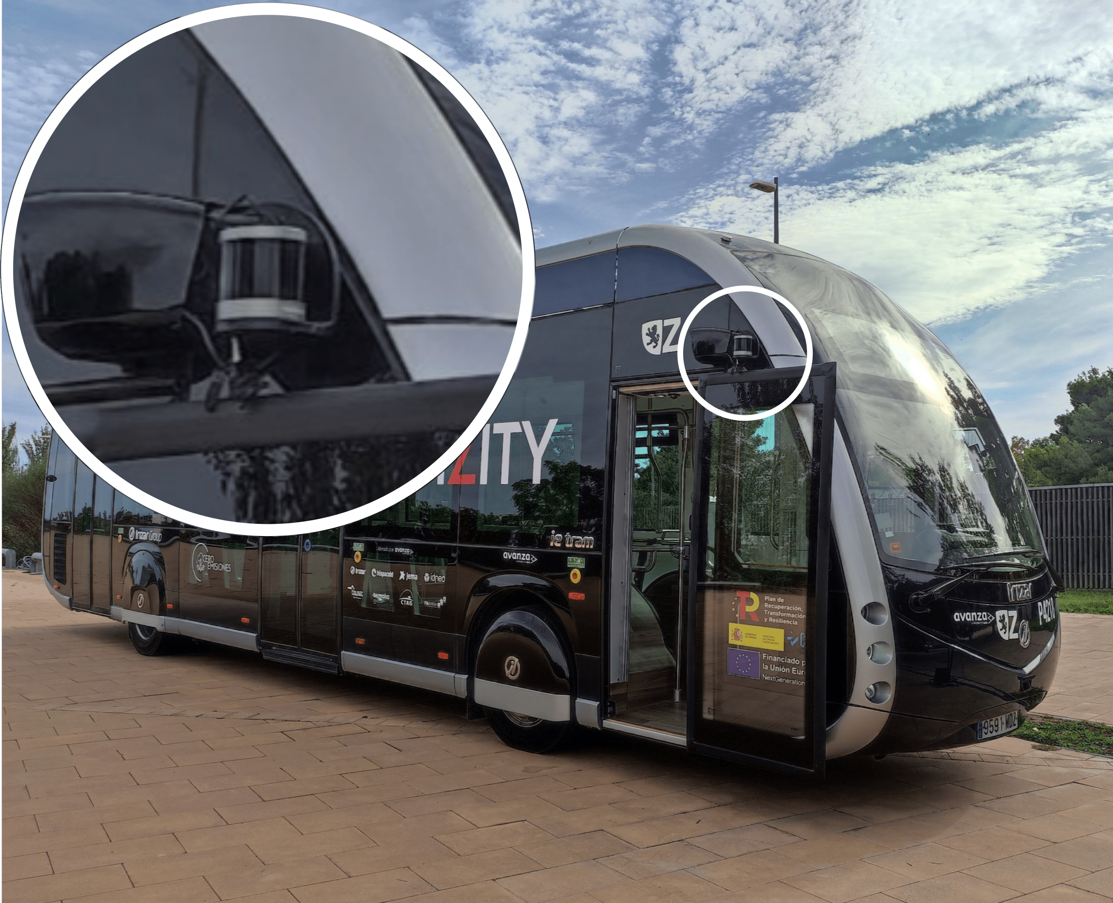
((a))

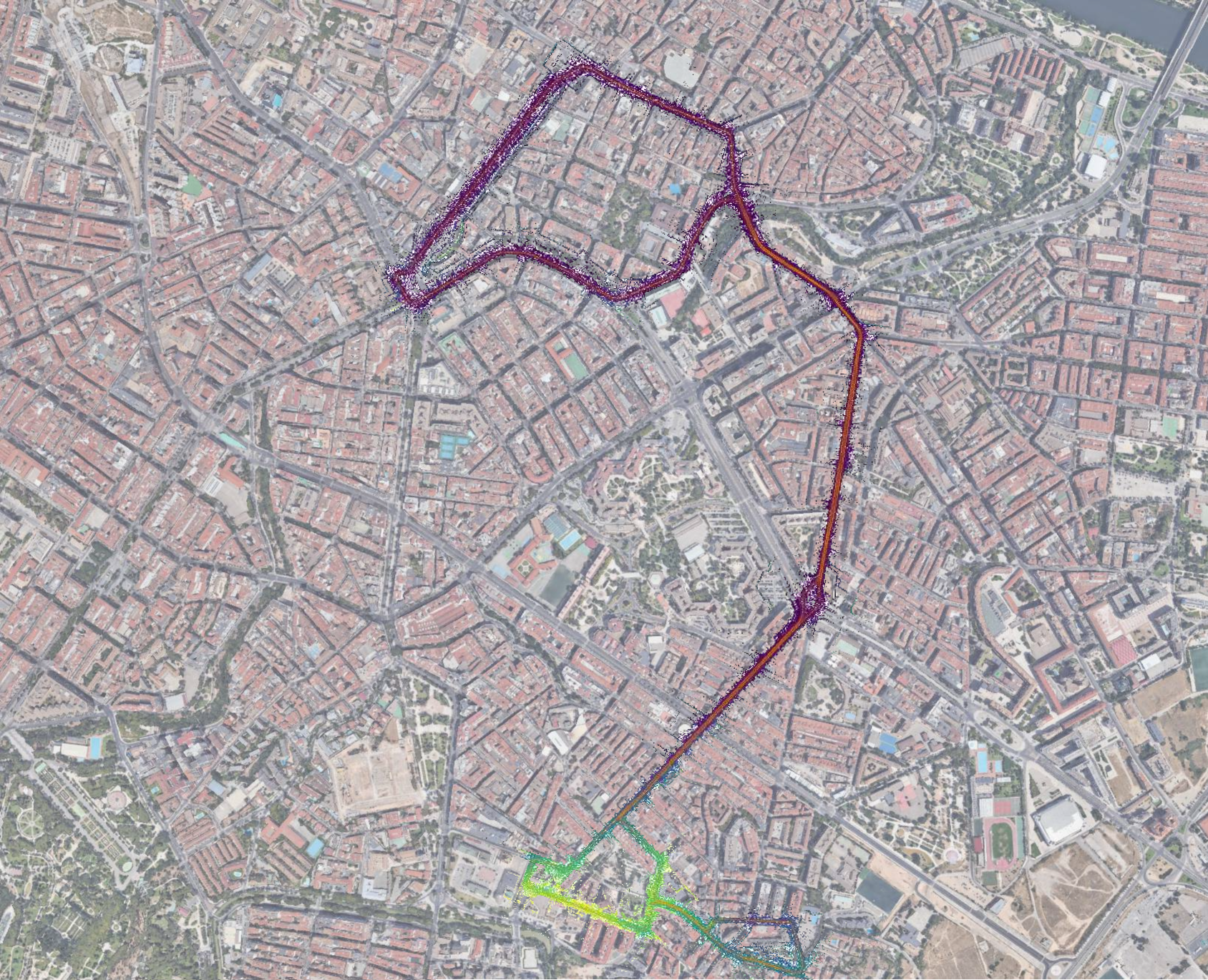
((b))

((c))

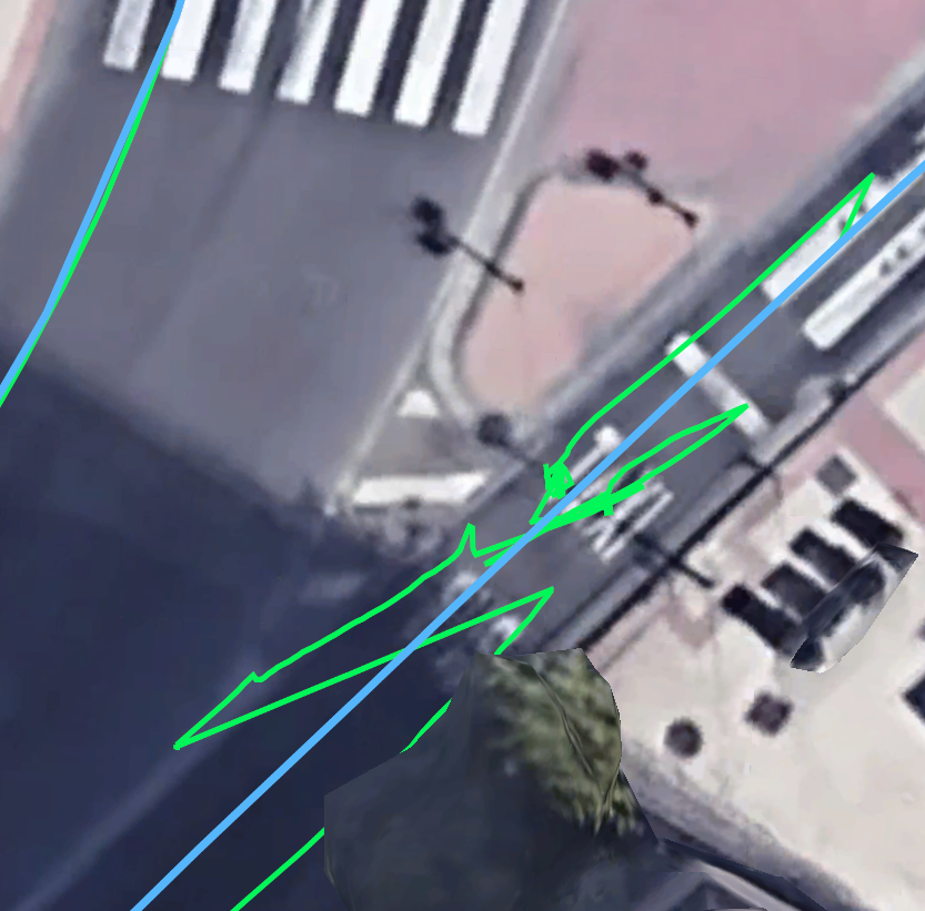
((d))

Figure 6: Results of the real-world experiment. (a) Platform and sensor setup. (b) Prior topo-metric model (colored by height, darker is lower). (c) Complete trajectory estimated by G-Loc. (d) Comparison between the raw GNSS (green) and the localization estimates (blue).

VI Conclusion

In this work we have presented G-Loc, a graph-based localization system whose design has been focused on autonomous urban driving. We propose a novel approach that leverages the result of a graph-SLAM process, not only the point clouds but also the underlying pose-graph representation. Our method seamlessly integrates GNSS, LIO measurements, and cloud-to-map registrations into a graph optimization framework, providing robust localization within a prior topo-metric map. We have tested G-Loc in different datasets and in a real-world automotive application, demonstrating its accuracy, robustness, and adaptability to different sensor configurations and environmental conditions (e.g., the lack of prior knowledge in some parts of the environment) without using costly SLAM techniques in previously mapped areas.

Long-term autonomy requires the sporadic execution of mapping to update the robot’s knowledge of the environment. This work sets the stage for the development of a long-term approach that integrates SLAM, map-based localization, and map update processes. Therefore, future work will aim at updating the prior model, which could be further refined and extended with online information, and reused later.

References

- [1] C. Cadena, L. Carlone, H. Carrillo, Y. Latif, D. Scaramuzza, J. Neira, I. Reid, and J. J. Leonard, “Past, present, and future of simultaneous localization and mapping: Toward the robust-perception age,” IEEE Trans. on Robotics, vol. 32, no. 6, pp. 1309–1332, 2016.
- [2] C. Campos, R. Elvira, J. J. G. Rodríguez, J. M. Montiel, and J. D. Tardós, “ORB-SLAM3: An accurate open-source library for visual, visual-inertial, and multimap slam,” IEEE Trans. on Robotics, vol. 37, no. 6, pp. 1874–1890, 2021.
- [3] N. Hughes, Y. Chang, S. Hu, R. Talak, R. Abdulhai, J. Strader, and L. Carlone, “Foundations of spatial perception for robotics: Hierarchical representations and real-time systems,” The Int. J. of Robotics Research, 2024.
- [4] G. Bresson, Z. Alsayed, L. Yu, and S. Glaser, “Simultaneous localization and mapping: A survey of current trends in autonomous driving,” IEEE Trans. on Intelligent Vehicles, vol. 2, no. 3, pp. 194–220, 2017.
- [5] J. A. Placed, J. Strader, H. Carrillo, N. Atanasov, V. Indelman, L. Carlone, and J. A. Castellanos, “A survey on active simultaneous localization and mapping: State of the art and new frontiers,” IEEE Trans. on Robotics, vol. 39, no. 3, pp. 1686–1705, 2023.
- [6] J. Levinson, M. Montemerlo, and S. Thrun, “Map-based precision vehicle localization in urban environments.” in Robotics: Science and systems, vol. 4. Atlanta, GA, USA, 2007, p. 1.
- [7] K. Yoneda, H. Tehrani, T. Ogawa, N. Hukuyama, and S. Mita, “Lidar scan feature for localization with highly precise 3D map,” in Intelligent Vehicles Symp. IEEE, 2014, pp. 1345–1350.
- [8] S. Kato, E. Takeuchi, Y. Ishiguro, Y. Ninomiya, K. Takeda, and T. Hamada, “An open approach to autonomous vehicles,” IEEE Micro, vol. 35, no. 6, pp. 60–68, 2015.
- [9] B. Nagy and C. Benedek, “Real-time point cloud alignment for vehicle localization in a high resolution 3D map,” in European Conf. on Computer Vision Workshops, 2018.
- [10] J. Levinson and S. Thrun, “Robust vehicle localization in urban environments using probabilistic maps,” in Inf. Conf. on Robotics and Automation. IEEE, 2010, pp. 4372–4378.
- [11] R. W. Wolcott and R. M. Eustice, “Robust LIDAR localization using multiresolution gaussian mixture maps for autonomous driving,” The Int. J. of Robotics Research, vol. 36, no. 3, pp. 292–319, 2017.
- [12] G. Wan, X. Yang, R. Cai, H. Li, Y. Zhou, H. Wang, and S. Song, “Robust and precise vehicle localization based on multi-sensor fusion in diverse city scenes,” in Int. Conf. on Robotics and Automation. IEEE, 2018, pp. 4670–4677.
- [13] F. Poggenhans, N. O. Salscheider, and C. Stiller, “Precise localization in high-definition road maps for urban regions,” in Int. Conf. on Intelligent Robots and Systems. IEEE, 2018, pp. 2167–2174.
- [14] E. Javanmardi, Y. Gu, M. Javanmardi, and S. Kamijo, “Autonomous vehicle self-localization based on abstract map and multi-channel lidar in urban area,” IATSS Research, vol. 43, no. 1, pp. 1–13, 2019.
- [15] T. Seco, M. T. Lázaro, J. Espelosín, L. Montano, and J. L. Villarroel, “Robot localization in tunnels: Combining discrete features in a pose graph framework,” Sensors, vol. 22, no. 4, 2022.
- [16] P. J. Besl and N. D. McKay, “Method for registration of 3-D shapes,” in Sensor fusion IV: control paradigms and data structures, vol. 1611. Spie, 1992, pp. 586–606.
- [17] L. Wang, Y. Zhang, and J. Wang, “Map-based localization method for autonomous vehicles using 3D-LIDAR,” IFAC PapersOnLine, vol. 50, no. 1, pp. 276–281, 2017.
- [18] R. P. D. Vivacqua, M. Bertozzi, P. Cerri, F. N. Martins, and R. F. Vassallo, “Self-localization based on visual lane marking maps: An accurate low-cost approach for autonomous driving,” Trans. on Intelligent Transportation Systems, vol. 19, no. 2, pp. 582–597, 2017.
- [19] W.-C. Ma, I. Tartavull, I. A. Bârsan, S. Wang, M. Bai, G. Mattyus, N. Homayounfar, S. K. Lakshmikanth, A. Pokrovsky, and R. Urtasun, “Exploiting sparse semantic HD maps for self-driving vehicle localization,” in Int. Conf. on Intelligent Robots and Systems. IEEE, 2019, pp. 5304–5311.
- [20] J. Jeong, Y. Cho, and A. Kim, “HDMI-LOC: Exploiting high definition map image for precise localization via bitwise particle filter,” Robotics and Automation L., vol. 5, no. 4, pp. 6310–6317, 2020.
- [21] R. W. Wolcott and R. M. Eustice, “Visual localization within lidar maps for automated urban driving,” in Int. Conf. on Intelligent Robots and Systems. IEEE, 2014, pp. 176–183.
- [22] P. Biber and W. Straßer, “The normal distributions transform: A new approach to laser scan matching,” in Int. Conf. on Intelligent Robots and Systems, vol. 3. IEEE, 2003, pp. 2743–2748.
- [23] P. Egger, P. V. Borges, G. Catt, A. Pfrunder, R. Siegwart, and R. Dubé, “Posemap: Lifelong, multi-environment 3D lidar localization,” in Int. Conf. on Intelligent Robots and Systems. IEEE, 2018, pp. 3430–3437.
- [24] G. Grisetti, R. Kümmerle, C. Stachniss, and W. Burgard, “A tutorial on graph-based SLAM,” Intelligent Transportation Systems Magazine, vol. 2, no. 4, pp. 31–43, 2010.
- [25] R. Dube, A. Cramariuc, D. Dugas, H. Sommer, M. Dymczyk, J. Nieto, R. Siegwart, and C. Cadena, “SegMap: Segment-based mapping and localization using data-driven descriptors,” The Int. J. of Robotics Research, vol. 39, no. 2-3, pp. 339–355, 2020.
- [26] C. Guo, M. Lin, H. Guo, P. Liang, and E. Cheng, “Coarse-to-fine semantic localization with HD map for autonomous driving in structural scenes,” in Int. Conf. on Intelligent Robots and Systems. IEEE, 2021, pp. 1146–1153.
- [27] K. Koide, S. Oishi, M. Yokozuka, and A. Banno, “Tightly coupled range inertial localization on a 3D prior map based on sliding window factor graph optimization,” arXiv preprint arXiv:2402.05540, 2024.
- [28] S. Thrun, “Probabilistic robotics,” Communications of the ACM, vol. 45, no. 3, pp. 52–57, 2002.
- [29] S. Macenski, T. Foote, B. Gerkey, C. Lalancette, and W. Woodall, “Robot operating system 2: Design, architecture, and uses in the wild,” Science Robotics, vol. 7, no. 66, 2022.
- [30] T. Shan, B. Englot, D. Meyers, W. Wang, C. Ratti, and D. Rus, “LIO-SAM: Tightly-coupled LiDAR inertial odometry via smoothing and mapping,” in Int. Conf. on Intelligent Robots and Systems. IEEE, 2020, pp. 5135–5142.
- [31] K. Koide, M. Yokozuka, S. Oishi, and A. Banno, “Voxelized GICP for fast and accurate 3D point cloud registration,” in Int. Conf. on Robotics and Automation. IEEE, 2021, pp. 11 054–11 059.
- [32] C. Forster, L. Carlone, F. Dellaert, and D. Scaramuzza, “On-manifold preintegration for real-time visual-inertial odometry,” IEEE Trans. on Robotics, vol. 33, no. 1, pp. 1–21, 2016.
- [33] G. Grisetti, R. Kümmerle, H. Strasdat, and K. Konolige, “g2o: A general framework for (hyper) graph optimization,” in Int. Conf. on Robotics and Automation. IEEE, 2011, pp. 9–13.
- [34] Z. Yan, L. Sun, T. Krajník, and Y. Ruichek, “EU long-term dataset with multiple sensors for autonomous driving,” in Int. Conf. on Intelligent Robots and Systems. IEEE, 2020, pp. 10 697–10 704.