High-mass star formation in the Large Magellanic Cloud triggered by colliding Hi flows

Abstract

The galactic tidal interaction is a possible mechanism to trigger the active star formation in galaxies. The recent analyses using the Hi data in the Large Magellanic Cloud (LMC) proposed that the tidally driven Hi flow, the L-component, is colliding with the LMC disk, the D-component, and is triggering high-mass star formation toward the active star-forming regions R136 and N44. In order to explore the role of the collision over the entire LMC disk, we investigated the I-component, the collision-compressed gas between the L- and D-components, over the LMC disk, and found that 74 % of the O/WR stars are located toward the I-component, suggesting their formation in the colliding gas. We compared four star-forming regions (R136, N44, N11, N77-N79-N83 complex). We found a positive correlation between the number of high-mass stars and the compressed gas pressure generated by collisions, suggesting that the pressure may be a key parameter in star formation.

1 Introduction

1.1 Active star formation induced by the galactic tidal interaction

Starburst is one of the critical processes in the galaxy’s evolution and the star formation history of the Universe. Many early studies suggested that tidal perturbations from nearby companions (1988A&A...203..259N; 1990PASJ...42..505F), galactic interactions including mergers (e.g., 1988ApJ...325...74S; 2008MNRAS.388L..10B), or cold gas accretion from the intergalactic medium (e.g.,1987ApJ...322L..59S) are possible mechanisms triggering the burst of star formation. 1998Natur.395..859G showed that galaxy mergers have excess infrared luminosity compared with isolated galaxies, lending support to the active star formation triggered by galaxy interactions. Subsequently, 2014A&A...566A..71L investigated 18 starburst dwarf galaxies using Hi data. They found that starburst dwarf galaxies have more asymmetric Hi morphologies than typical dwarf irregulars, and $\sim$80 % of the starburst dwarf galaxies are interacting galaxies with at least one potential companion within 200 kpc. Thus, these previous works suggest that some external mechanism induced by galactic interaction triggers the starburst. In addition, numerical simulations of galaxy interactions show that interactions/mergers between gas-rich dwarfs formed irregular blue compact dwarfs (BCDs) , including IZw 18, which hosts starburst (2008MNRAS.388L..10B). BCDs have low metallicity (0.1$\geq$$Z$/$Z_{\rm\odot}$$\geq$0.02) and are similar to the environment where the first stars formed in the early Universe (1972ApJ...173...25S). Therefore, elucidation of the triggering mechanism of active star formation in dwarf galaxies has the potential to promote understanding of the origin of starbursts in the early Universe. Most of the interacting galaxies are, however, distant, and it is difficult to resolve individual clouds and investigate their physical properties in detail, except for recent ALMA studies toward the nearby interacting system, such as the Antennae Galaxies (e.g., 2014ApJ...795..156W; 2021PASJ...73S..35T; 2021PASJ...73..417T).

The present study focuses on the Large Magellanic Cloud (LMC). The LMC is one of the nearest interacting dwarf galaxies (distance 50$\pm$1.3 kpc;2013Natur.495...76P) and is almost face-on with an inclination of $\sim$20–30 deg. (e.g., 2010A&A...520A..24S). Thus, the LMC is an optimal laboratory for investigating the active star formation mechanisms across cosmic history, covering a wide spatial-dynamic range from a galactic scale (kpc scale) down to a cluster scale (10–15 pc). The mean metallicity of the LMC is approximately half of the solar metallicity (0.3–0.5 $Z_{\rm\odot}$; 1992ApJ...384..508R; 1997macl.book.....W), which is close to the mean metallicity of the interstellar medium during the time of peak star formation (redshift z$\sim$1.5; 1999ApJ...522..604P). The LMC is an optimal laboratory for investigating the active star formation mechanisms through a wide spatial-dynamic range from a galactic scale (kpc scale) down to a stellar cluster scale (10–15 pc).

There are many active star-forming regions over the LMC, which have been intensively studied (N77-N79-N83 complex: e.g., 2017NatAs...1..784O; Nayak et al. 2019, N159: Chen et al. 2010; Saigo et al. 2017; Fukui et al. 2019; Tokuda et al. 2019, N11: e.g., Walborn & Parker 1992; Celis Pena et al. 2019, N44; e.g., Chu et al. 1993; Chen et al. 2009, N206: e.g., Romita et al. 2010, N51: e.g., Lucke & Hodge 1970; Chu et al. 2005, N105:e.g., Epchtein et al. 1984; Oliveira et al. 2006, N113: e.g., Brooks & Whiteoak 1997, N120: e.g., Lucke  Hodge 1970; N144; e.g., Lortet & Testor 1988 etc. cataloged by Henize 1956 listed in ascending R.A. order). Above all, recent works by Fukui et al. 2017 and Tsuge et al. 2019 revealed evidence for the triggered formation of the massive young cluster R136, the Hii region N44 and some of the other high-mass stars in the LMC. These authors suggested that the tidal interactions induced colliding Hi gas flows in the LMC.

1.2 The interacting two velocity components

Many observational studies support the LMC–SMC interaction from the stellar proper motion of the Magellanic Bridge. The Magellanic Bridge is a structure of Hi gas that extends like a bridge between the LMC and the SMC, believed to have formed due to the gravitational interaction between the LMC and SMC (Murai & Fujimoto, 1980; Gardiner et al., 1994). The latest observations of stellar proper motion using GAIA suggested a close encounter and collision between the SMC and LMC $\sim$0.2 Gyr ago (e.g., 2019ApJ...874...78Z; 2013ApJ...764..161K). The authors of Kallivayalil et al. (2013) revealed the proper motions of stars in the Magellanic Bridge and found that the stars moved from the SMC to the LMC. They compared their results with a numerical model of the Magellanic Bridge formation and discovered that the observations agree with a model in which the SMC-LMC collision occurs with an impact parameter of less than a few kpc (e.g., 2018ApJ...867L...8O).

The star formation history estimated from photometry of stellar populations also supports the LMC–SMC interaction as shown by numerical simulations (e.g., 2009ApJ...705.1260N; 2020A&A...641A.134S; 2005MNRAS.358.1215P; 2005AJ....130.1083M; 2009AJ....138.1243H; 2018ApJ...866...90C; 2022ApJ...927..153C; 2018ApJ...864...55Z). Especially, 2009ApJ...705.1260N and 2009AJ....138.1243H support the recent interaction within 1 Gyr. These simulation models need to be confronted with observations not only of the stars but also of the distribution and kinematics of the gas that forms stars. This contrasts with previous simulation studies, which are based on comparisons with observations of stars only. 2022ApJ...927..153C also suggests that the best model is one in which the latest collision occurred within  0.25 Gyr with the collision parameter of 10 kpc. We should note that the kinematics and distribution of the stars are the product in a longer time scale than the gas. Fukui et al. (2018) estimated the ionization velocity by O-stars to be 5 km/s by comparing observational results of molecular clouds associated with massive star clusters of various ages. Based on this velocity, it is estimated that molecular clouds within 50 pc of the star cluster will be ionized after 10 million years, making verifying the gas involved in star formation challenging. It is, therefore, essential to look at the associated gas component, which reflects events in a short time scale of 10 Myr, in order to elucidate detailed dynamics of the interaction and its relationship to recent star formation

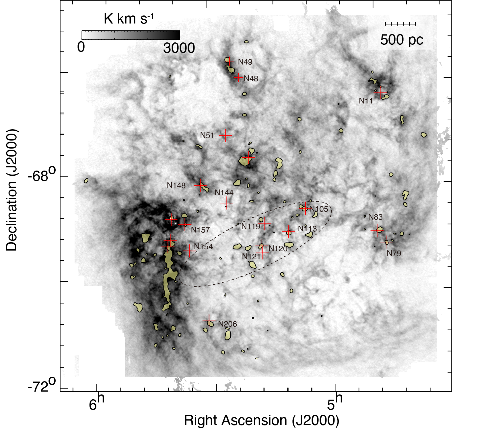
Figure 1: The Hi integrated intensity maps with the integration velocity range of $V_{\rm offset}$=$-$101.1–29.9 km s${}^{-1}$. The yellow shaded areas are the regions where ${}^{12}$CO($J$=1–0) intensity obtained with NANTEN is greater than 1.5 $\sigma$ (1.48 K km s${}^{-1}$) with the same velocity range. Plus signs show the positions of luminous Hii regions (S${}_{H\alpha}$ $>$ 1$\times$10${}^{4}$ erg cm${}^{-2}$ s${}^{-1}$ sr${}^{-1}$; Ambrocio-Cruz et al. 2016). The dashed line shows the optical boundary of the stellar bar.

1992A&A...263...41L identified two velocity Hi components based on Hi observations at 15 $\arcmin$ resolution (corresponding to $\sim$225 pc at the distance of the LMC) and named the two as the L-component and the D-component, where the L-component has smaller velocity by 50 km s${}^{-1}$ than the D-component. Subsequently, Hi observations at a higher spatial resolution of 1 $\arcmin$ were conducted by 2003ApJS..148..473K, and Hi shells and holes were investigated in detail over the LMC, as shown in Figure 1. The presence of multiple components results in an asymmetric intensity distribution of the Hi gas shown in Figure 1. Signs for the L- and D-components were also recognized in the high-resolution data. In contrast, the previous studies including 2003MNRAS.339...87S and 2015A&A...573A.136I did not investigate the physical properties of the two components.

Most recently, the two components were reviewed in the light of the colliding Hi flows which triggered the formation of Young Massive Clusters (YMCs) by 2017PASJ...69L...5F (hereafter Paper I) and by 2019ApJ...871...44T (hereafter Paper II). YMCs are astronomical objects characterized by total cluster masses typically exceeding 10${}^{4}$ $M_{\odot}$ and containing many high-mass stars within a radius of 1 pc (Portegies Zwart et al., 2010) These works revealed that the L- and D-components are colliding toward two outstanding clusters/Hii regions, R136 in the Hi Ridge and N44 in the northern part. They suggested that the collisional trigger likely forms both.

Conventionally, the rotation curve of the LMC was obtained from the Hi data, where the L- and D-components are mixed up. In their study, Paper II developed a method to decompose the L- and D-components by subtracting the galactic rotation, which laid a foundation for a detailed kinematical study of Hi in the LMC. This rotation curve is consistent with the latest results presented by Oh et al. (2022). They thereby confirmed the original suggestion by 1992A&A...263...41L on the two components, and identified observational signatures of the collision between the two components as follows; i. the complementary spatial distribution between the L- and D- components and ii. the intermediate velocity component (hereafter the I-component) connects the two components in velocity space, which supports the collisional interaction of the L- and D-components. By using the Atacama Large Millimeter/submillimeter Array (ALMA), 2019ApJ...886...14F; 2019ApJ...886...15T found massive filamentary clouds toward the N159 region in the Hi Ridge, holding high-mass star formation, which shows cloud collision signatures at a few pc in the CO clouds.

Based on these signatures, Papers I and II, 2019ApJ...886...14F, and 2019ApJ...886...15T argued that the collision between the L- and D-components worked as a formation mechanism of $\sim$400 high-mass stars including R136, N159, and N44. This scenario is supported by the numerical simulations which elaborate the observational characteristics of a cloud-cloud collision (e.g., 1992PASJ...44..203H; 2010MNRAS.405.1431A; 2014ApJ...792...63T; 2018PASJ...70S..58T; 2018PASJ...70S..54S; 2018PASJ...70S..53I; 2018PASJ...70S..59K; 2021PASJ...73S.385S; 2021ApJ...908....2M; 2018ApJ...859..166F; 2021PASJ...73S.405F; see also for a review 2021PASJ...73S...1F).

The origin of the L-component is most likely the tidal interaction between the LMC and the SMC at their close encounter, which occurred $\sim$0.2 Gyr ago. The gas stripped from both the LMC and the SMC by the tidal force is expected to fall down currently to the LMC disk, which causes the L- and D-components. This scenario is supported by the detailed numerical simulations of the tidal interaction by 2007PASA...24...21B (see also 2007MNRAS.381L..16B; 2005MNRAS.356..680B; 2014MNRAS.443..522Y). Papers I and II developed the discussion along the tidal interaction and argued for the gas injection from the SMC into the LMC based on the low dust-to-gas ratio. Paper I and Paper II estimated the metal amount by a comparison of dust optical depth at 353 GHz ($\tau$353) measured by $Planck/IRAS$ telescopes (Planck Collaboration 2014) and the intensity of Hi ($W$(Hi)). The authors found a factor of two differences in the dust-to-gas ratio between the L-component and the D-component. That difference corresponds to the difference in metallicity if we assume that the dust-to-gas ratio is constant in the LMC. The L-component is estimated to have about half the metallicity of the D-component due to gas inflow from the SMC (Paper I).

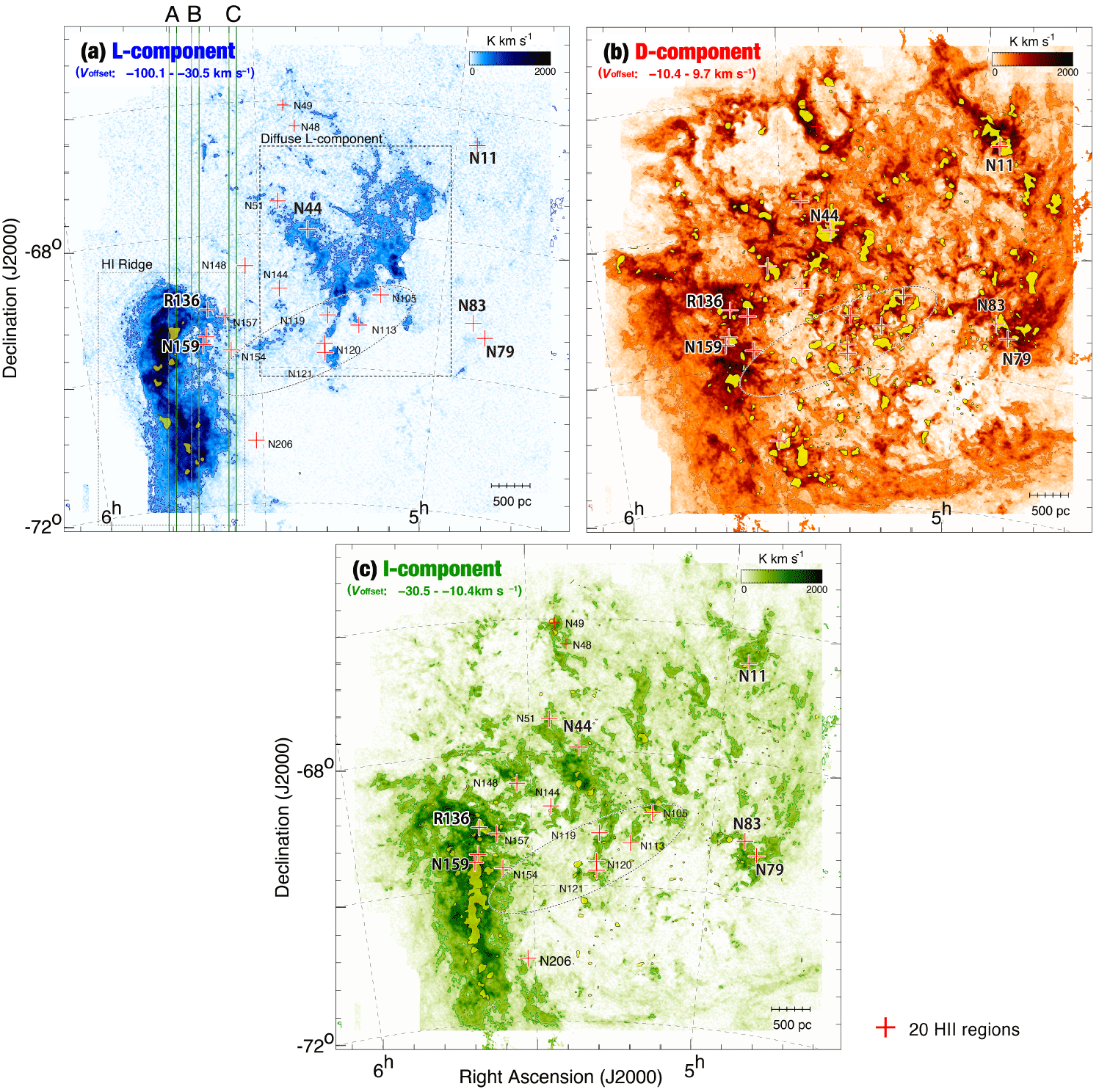
Figure 2: The Hi integrated intensity maps of (a) the L-component, (b) the D-component, and (c) the I-component. The integration velocity range is $V_{\rm offset}$=$-$101.1–$-$30.5 km s${}^{-1}$ for the L-component, $V_{\rm offset}$=$-$10.4–9.7 km s${}^{-1}$ for the D-component, and $V_{\rm offset}$=$-$30.5–$-$10.4 km s${}^{-1}$ for the I-component. The lowest contour level and intervals are 192 K km s${}^{-1}$ (15 $\sigma$) and 769 K km s${}^{-1}$ (60 $\sigma$) for (a) and 279 K km s${}^{-1}$ (40 $\sigma$) and 419 K km s${}^{-1}$ (60 $\sigma$) for (b) and (c). The yellow shaded areas in three panels are the regions with ${}^{12}$CO($J$=1–0) intensity greater than 1.5 $\sigma$ with the same velocity range. Plus signs show the positions of luminous Hii regions (S${}_{H\alpha}$ $>$ 1$\times$10${}^{4}$ erg cm${}^{-2}$ s${}^{-1}$ sr${}^{-1}$; Ambrocio-Cruz et al. 2016). The green lines in (a) show the integration ranges in R.A. in Figure LABEL:fig21.

1.3 The I-component: a possible tracer of the colliding Hi flows and triggered star formation

We defined the I-component, whose velocity is intermediate between the L- and D-components in Paper II. We interpret that the I-component is the mixture of the decelerated L-component and the D-component in the collisional interaction. According to the picture, molecular gas is formed by the density increase in the compressed interface layer, as shown in the synthetic observations by 2018ApJ...860...33F of the colliding Hi flows which were numerically simulated by 2012ApJ...759...35I. It is likely that the molecular gas leads to the formation of massive stellar clusters (2021ApJ...908....2M). Such a high-density part of the I-component is found in the CO distribution toward R136, N159, and N44 (Figures 8 and 9a and Paper II), suggesting the possibility that high-mass star formation is triggered by the colliding Hi flows over the LMC. Tsuge et al. (2021) found that the number density of colliding gas and collision velocity are important parameters, and there is a positive correlation between the collisional compression pressure calculated from the density and velocity and the mass of the stellar cluster. The present study aims to explore the role of the collisional interaction of the Hi gas and its relationship with high-mass star formation over the whole LMC.

To achieve this goal, we analyze Hi data comprehensively. We summarize the quantitive comparison of spatial distributions of the I-component and high-mass stars in Section 3.3. A detailed investigation of the observational signatures of Hi collisions in the N11 and N77-N79-N83 complex in Section 4.1.3 and LABEL:sec:4.1.4, respectively. N11 is located at the edge of supergiant shell 1 (Dawson et al. 2013) and is the oldest Hii region among these regions. N77-N79-N83 complex is located at the origin of the western tidal arm and, N79 is noted as a feature rival to 30Dor (Ochsendorf 2017). We cover a wide range of locations and surrounding environments (density of colliding gas, collision velocities, collisional compression pressures, and metallicity) in the LMC, as shown in Figure 1. These differences can influence important physical quantities related to star formation and molecular cloud formation, such as gas mass accretion rates and cooling efficiency.

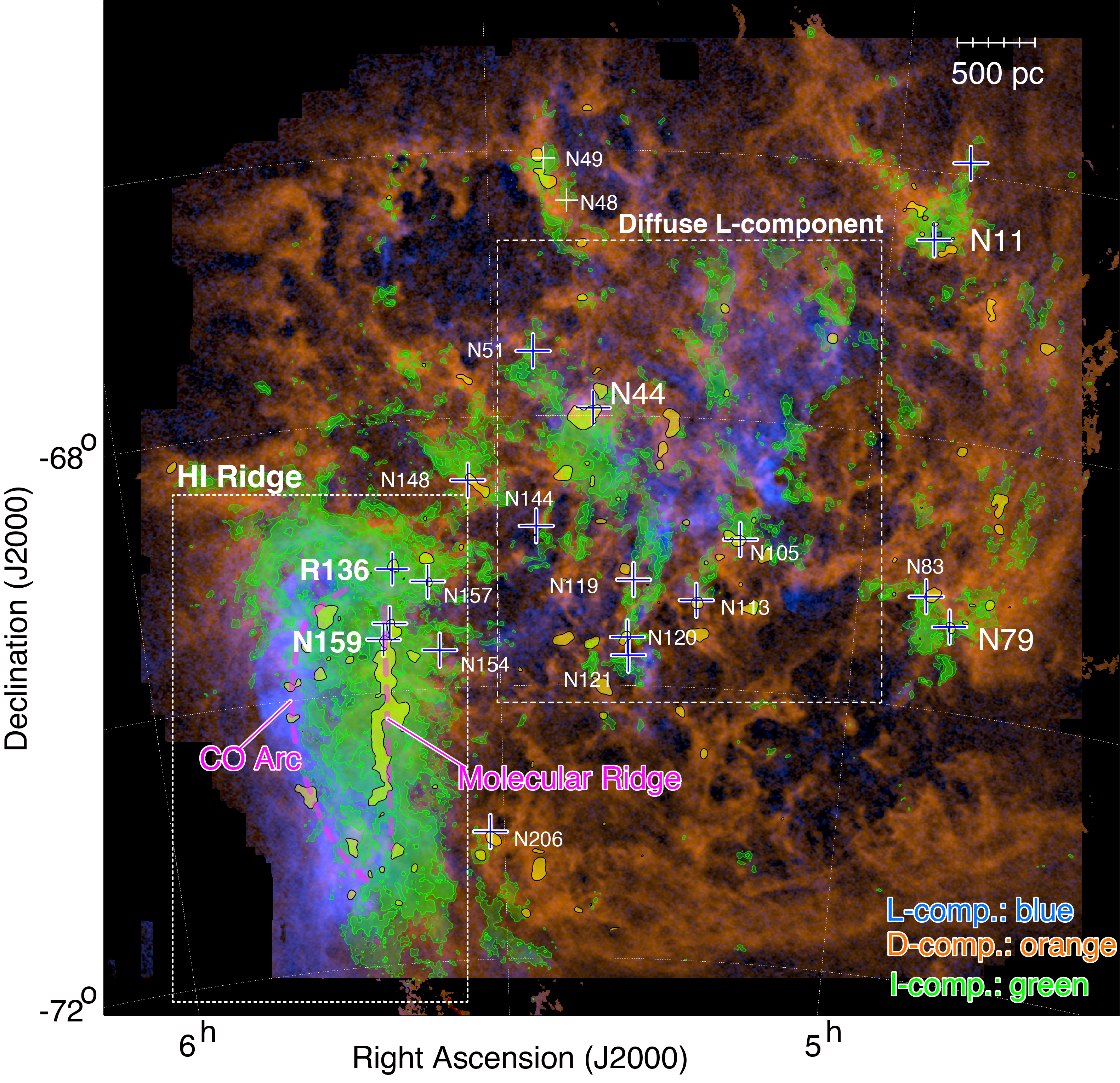
Figure 3: Hi intensity map of the I-component by contours superposed on the L- and D-components image. The velocity ranges of three components are the same as in Figure 1. The contour levels are 300, 500 and 1000 K km s${}^{-1}$. Plus signs show the positions of luminous Hii regions (S${}_{H\alpha}$ $>$ 1$\times$10${}^{4}$ erg cm${}^{-2}$ s${}^{-1}$ sr${}^{-1}$; 2016MNRAS.457.2048A). Molecular clouds of N48 and N49, which are located between two SGSs, LMC 4 and LMC 5 are also shown by crosses. The shaded areas in yellow are the the regions where ${}^{12}$CO($J$=1–0) intensity obtained with NANTEN is greater than 1.5 $\sigma$ (1.48 K km s${}^{-1}$) with the same velocity range. The magenta dashed lines shows the Molecular Ridge and CO-Arc region.

2 Datasets

We used the original angular resolution to compare the spatial distributions, whereas we smoothed the data and matched the resolution of CO and Hi to calculate physical parameters.

2.1 HI

We used archival data of Hi 21 cm line emission of the whole LMC obtained with Australia Telescope Compact Array (ATCA) and Parkes telescope (2003ApJS..148..473K). They combined the Hi data obtained by ATCA (Kim et al. 1998) with those obtained with the Parkes multi beam receiver with a resolution of 14$\arcmin$–16$\arcmin$(1997PASA...14..111S). The angular resolution of the combined Hi data is 60$\arcsec$ (corresponding to $\sim$15 pc at the distance of the LMC). The rms noise level is 2.4 K at a velocity resolution of 1.649 km s${}^{-1}$. More detailed descriptions of the observations are given by 2003ApJS..148..473K.

2.2 CO

${}^{12}$CO($J$=1–0) data obtained with the NANTEN 4 m telescope (1999PASJ...51..745F; 2008ApJS..178...56F; 2001PASJ...53..971M) are used for a large-scale analysis. These observations cover a 6${}^{\circ}$$\times$6${}^{\circ}$ area, including the whole optical extent of the LMC, are suitable for the comparison with the kpc scale Hi dynamics. The half-power beam width was 2$\farcm$6 (corresponding to $\sim$40 pc at the distance of the LMC) with a regular grid spacing of 2$\farcm$0, and a velocity resolution was 0.65 km s${}^{-1}$.

We also used ${}^{12}$CO($J$=1–0) data of the Magellanic Mopra Assessment (MAGMA; 2011ApJS..197...16W) for a small-scale analysis in each star-forming region. The angular resolution was 45$\arcsec$ (corresponding to 11 pc at the distance of the LMC), and the velocity resolution was 0.526 km s${}^{-1}$. The MAGMA survey does not cover the whole LMC, and the observed area is limited to the individual CO clouds detected by the NANTEN survey.

2.3 H$\alpha$

We used the H$\alpha$ data obtained by the Magellanic Cloud Emission-Line Survey (MCELS; 1999IAUS..190...28S). The dataset was obtained with a 2048$\times$2048-pixel CCD camera on the Curtis Schmidt Telescope at Cerro Tololo Inter-American Observatory. The angular resolution was $\sim$3$\arcsec$–4$\arcsec$ (corresponding to $\sim$0.75–1.0 pc at a distance of the LMC). We also use the archival data of H$\alpha$ provided by the Southern H-Alpha Sky Survey Atlas (SHASSA; 2001PASP..113.1326G) to define the region where UV radiation is locally enhanced by star formation.

3 Observational Results

3.1 Spatial- and velocity distributions of HI gas at a kpc scale

The method of derivation of the three components is summarized below. The L- and D-components were decomposed over the whole LMC for the first time at a high angular resolution of 1$\arcmin$ (corresponding to $\sim$15 pc at the distance of the LMC) in Papers I and II. The rotation curve of the D-component was then derived in Paper II, which corresponds to the LMC disk. The rotation curve differs from the previous works (2003ApJS..148..473K) which treated all the Hi components as the LMC disk. The present rotation curve includes only the D-component. We then defined $V_{\rm offset}$ as a relative velocity from the rotational velocity of the D-component ($V_{\rm offset}$ = $V_{\rm LSR}$$-$$V_{\rm D}$; $V_{\rm D}$ = the projected rotation velocity of the D-component). The integration ranges are $V_{\rm offset}$: $-$100.1–$-$30.5 km s${}^{-1}$ for the L-component; and $V_{\rm offset}$: $-$30.5 – $-$10.4 km s${}^{-1}$ for the I-component; $V_{\rm offset}$: $-$10.4–9.7 km s${}^{-1}$ for the D-component as explained in Paper II. We also made a histogram of Hi gas toward the northern part of the Hi Ridge region, as shown in Figure LABEL:fig16 of Appendix 1. This histogram illustrates that the velocities $-$30 km s${}^{-1}$ and $-$10 km s${}^{-1}$ well correspond to the boundaries between the three components.

Figure 2 shows overlays of the distribution of the three Hi components with the major 20 star-forming regions ($S_{\rm H\alpha}$ $>$ 1$\times$10${}^{4}$ erg cm${}^{-2}$ s${}^{-1}$ sr${}^{-1}$; Ambrocio-Cruz et al. 2016) over the whole LMC. We present the distributions of the three components in Figures 2(a), 2(b), and 2(c), which show the spatial distributions of the L-, D-, and I-components, respectively. Figure 3 is an overlay of high integrated intensity areas ($W$(Hi)$>$300 K km s${}^{-1}$) of the three distributions. The distributions of the L-, I-, and D-components are significantly different, while these three components partially show similar distribution. All three components, L, I, and D, are concentrated in the Hi Ridge region. While the D-component extends across the entire galaxy, the L-component is concentrated in the southeastern Hi Ridge and the northwestern Diffuse L-component directions. The I-component is concentrated toward regions where the intensity of the D-component is outstanding. The spatial distribution of active Hii regions which have surface luminosity $S_{\rm H\alpha}$ greater than 1$\times$10${}^{4}$ erg cm${}^{-2}$ sr${}^{-1}$ (2016MNRAS.457.2048A) resembles the strong I-component.

3.2 Detailed properties of the three HI components

The L-component is composed of two kpc-scale extended features. One is the Hi Ridge region located in the southeast region, which includes two major elongated CO components, i.e., the Molecular Ridge and the CO-Arc (1999PASJ...51..745F; 2001PASJ...53..971M, magenta dashed lines of Figure 3). The other is the Diffuse component extending toward the northwest as shown in the dashed box of Figure 2a (hereafter the Diffuse L-component as in Paper II). The I-component is distributed along the western rim of Hi Ridge’s L-component and the Diffuse L-component’s periphery, as shown in Figure 3. The I-component is also located toward the southern end of the western arm (2003MNRAS.339...87S), including N77-N79-N83 complex and N11, where we find only weak signs of the L-component. The I-component shows good correspondence with the Molecular Ridge, while it has little resemblance with the CO-Arc. Finally, the D-component is distributed over the whole LMC.

Hi and H${}_{2}$ masses ($M$(Hi) and $M$(H${}_{2}$)) of the L-, D-, and I-components are summarized for the whole LMC and the Hi Ridge region, respectively, in Table 1. We calculated the mass of the Hi gas in the assumption that Hi emission is optically thin as follows,

$${M{\rm(HI)}=m_{p}\Omega D^{2}\Sigma_{i}N_{i}({\rm HI})},$$ (1)

where $m_{p}$ is the mass of hydrogen. $D$ is the distance to the source in cm, equal to 50 kpc, $\Omega$ is the solid angle subtended by a unit grid spacing of a square pixel, and $N_{i}$(HI) is the atomic hydrogen column density for each pixel in cm${}^{-2}$.

$${N({\rm H{\sc I})}=1.8224\times 10^{18}\int\Delta T_{\rm b}\it dv\ \rm{[cm^{-2}]},}$$ (2)

where $T_{\rm b}$ is the observed Hi brightness temperature (K). We also derived the masses of the molecular clouds using the $W_{\rm CO}$–$N$(H${}_{2}$) conversion factor ($X_{\rm CO}$ = 7.0$\times$10${}^{20}$ cm${}^{-2}$ (K km s${}^{-1}$)${}^{-1}$; 2008ApJS..178...56F). We used the equation as follows,

$${M{\rm(H_{2})}=m_{\rm H}\mu\Omega D^{2}\Sigma_{i}N_{i}({\rm H2}),}$$ (3)

where $m_{\rm H}$ is the mass of the hydrogen atom, $\mu$ is the mean molecular weight relative to a hydrogen atom, $D$ is the distance to the source in cm, equal to 50 kpc, $\Omega$ is the solid angle subtended by a unit grid spacing of a square pixel, and $N_{i}$(H${}_{2}$) is the hydrogen molecule column density for each pixel in unit of cm${}^{-2}$. We adopt $\mu$ = 2.7 to take into account the $\sim$36% abundance by mass of helium relative to hydrogen molecule.

$${N(H_{2})=X_{\rm CO}\times W(^{12}CO(J=1-0)),}$$ (4)

where $W_{\rm CO}$ is the integrated intensity of ${}^{12}$CO($J$=1–0) and $N$(H${}_{2}$) is the column density of molecular hydrogen. The masses of atomic hydrogen and molecular hydrogen are 0.3$\times$10${}^{8}$ $M_{\rm\odot}$ and 0.3$\times$10${}^{7}$ $M_{\rm\odot}$ for the L-component, 0.8$\times$10${}^{7}$ $M_{\rm\odot}$ and 0.9$\times$10${}^{7}$ $M_{\rm\odot}$ for the I-component, and 1.8$\times$10${}^{8}$ $M_{\rm\odot}$ and 2.0$\times$10${}^{7}$ $M_{\rm\odot}$ for the D-component. The I-component likely consists of the mass converted from the L- and D-components.

We calculated the molecular mass fraction ($f_{\rm mol}$) of the Hi Ridge region with

$$f_{\rm mol}=M({\rm H_{2}})/M({\rm HI}).$$ (5)

$f_{\rm mol}$ of the L-, I-, and D-components is 15%, 30%, and 9%, respectively. $f_{\rm mol}$ of the I-component is enhanced and is three times higher than that of the D-component in the Hi Ridge. This suggests that the I-component of the Hi Ridge region and molecular clouds are effectively formed in the Hi Ridge region.

Table 1: Mass of hydrogen gas over the whole LMC

HI component		M(Hi)	$M$(H${}_{2}$)	$f_{\rm mol}$
		[$M_{\odot}$]	[$M_{\odot}$]	[$\%$]
The whole LMC	L-comp.	0.3$\times$10${}^{8}$	0.3$\times$10${}^{7}$	$\sim$10
	I-comp.	0.8$\times$10${}^{8}$	0.9$\times$10${}^{7}$	$\sim$10
	D-comp.	1.8$\times$10${}^{8}$	2.0$\times$10${}^{7}$	$\sim$10
The Hi Ridge	L-comp.	2.5$\times$10${}^{7}$	3.8$\times$10${}^{6}$	$\sim$15
	I-comp.	3.4$\times$10${}^{7}$	1.1$\times$10${}^{7}$	$\sim$30
	D-comp.	4.6$\times$10${}^{7}$	4.3$\times$10${}^{6}$	$\sim$9

Figure 4 shows the first moment distributions of the three components. The first moment is the intensity-weighted velocity following the equation of $\Sigma$($I$ $\times$ $v$)/$\Sigma$($I$), where $I$ is the intensity of emission and $v$ is $V_{\rm offset}$, which is defined as $V_{\rm offset}$ = $V_{\rm LSR}$$-$$V_{\rm LSR}$ (the D-component) (Papers I and II). Figure 4(a) shows the first moment of the L-component. For the Hi Ridge region, there is a velocity gradient from the east to the west. The typical velocity of the eastern side is $-$60 km s${}^{-1}$, which increases to $-$30 km s${}^{-1}$ on the western side. Figure 4(b) shows the first moment of the D-component, where no systematic change is found. Figure 4(c) indicates the first moment of the I-component. The first moment of the I-component exhibits lower velocities, particularly in regions where it spatially overlaps with the L-component.

Figure 4(d) shows histograms of the first moment of the I-component. The median value of the first moment is $\sim$$-$20.5 km s${}^{-1}$ at the positions where the integrated intensity of the L-component is more extensive than 300 K km s${}^{-1}$. Meanwhile, the median of the first moment toward the other regions is $\sim$$-$16.5 km s${}^{-1}$. Thus, the blue-shifted velocity of the I-component is affected by the dense part of the L-component, and the red-shifted velocity of the I-component is affected by the D-component. This comparison indicates that the I-component is strongly influenced by the L-component, which is consistent with the fact that the I-component is induced by the interaction driven by the L-component.

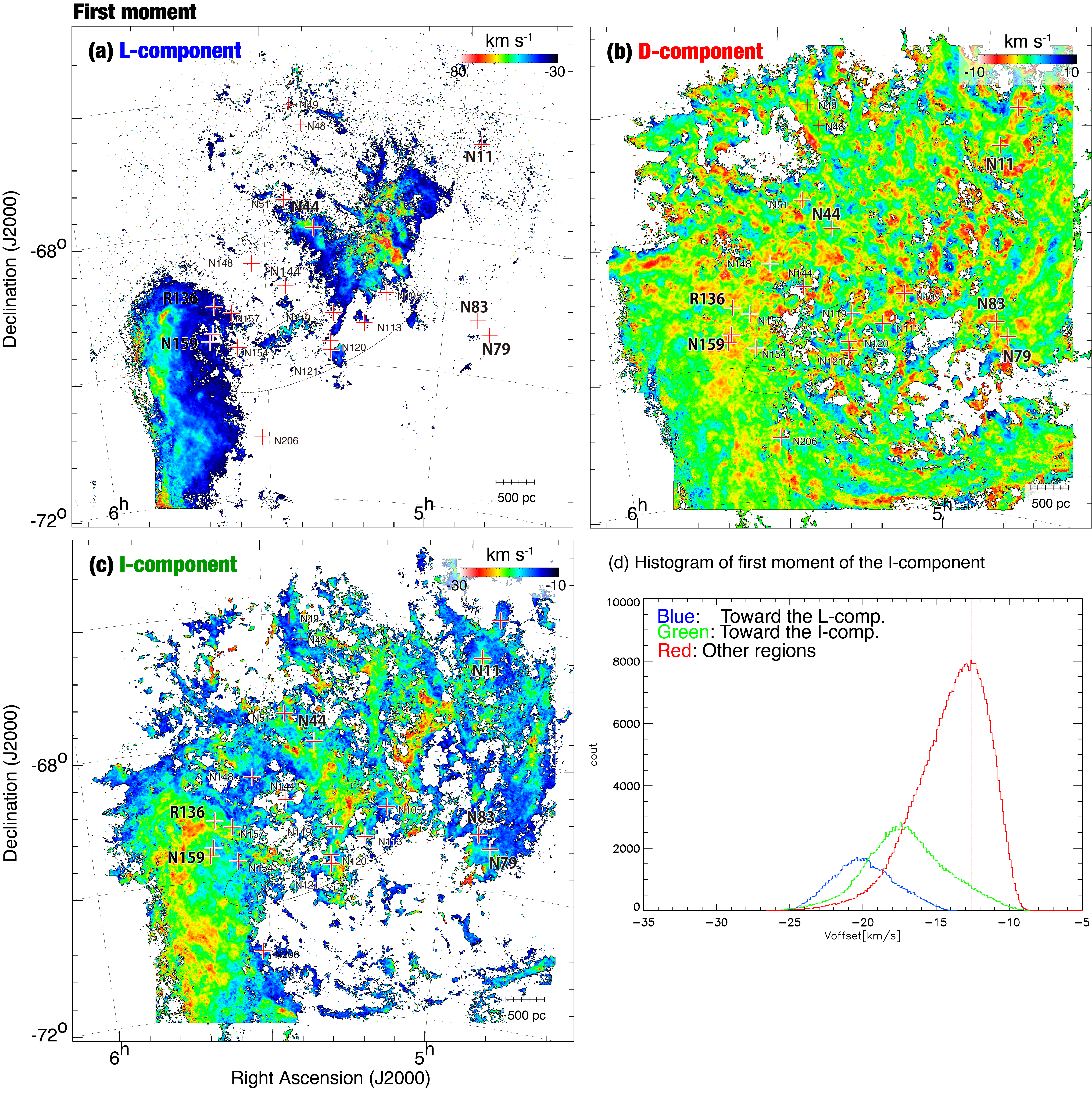
Figure 4: First moment map of Hi over the whole LMC. Velocity ranges using for calculating momentum are $V_{\rm offset}$=$-101.1$–$-$30.5 km s${}^{-1}$ (the L-component) for (a); $V_{\rm offset}$=$-10.4$–$-$9.7 km s${}^{-1}$ (the D-component) for (b); $V_{\rm offset}$=$-30.5$–$-$10.4 km s${}^{-1}$ (the I-component) for (c). The symbols are the same as in Figure 1. (d) Histograms of first-moment map of the I-component. The histograms of the first moment at the positions where the integrated intensity of the L-component is larger than 300 K km s${}^{-1}$ are shown in blue. The histograms of the first moment at the positions where the integrated intensity of the I-component is larger than 300 K km s${}^{-1}$ are shown in green. The histograms of other regions which is dominated by the D-component are shown in red. Dashed lines show the median value of the first-moment map.

3.3 Comparison of the I-component and high-mass stars

We find by eye inspection that the I-component shows the best association with the major star-forming regions among the three. This motivates us to explore further details of the association with the high-mass stars with the I-component in the following. In Figure 5(a), we compare the spatial distributions of the I-component and 697 O/WR stars (hereafter O/WR stars) (2009AJ....138.1003B). These O/WR stars allow us to examine the correlation more extensively than the major star-forming regions. In Figure 5(b), we also show the distribution of the H$\alpha$ emission overlaid on the I-component, which traces the effect of the ionization/feedback on the Hi by the O/WR stars.

To inspect the feedback effects due to ionization/stellar winds by the O/WR stars, we compare spatial distributions of H$\alpha$ emission and Hi gas toward the three regions around the R136, N11, and N77-N79-N83 complex at a 10–100 pc scale. Figures 5(c), 5(d), and 5(e) show enlarged views of the Hi toward N11, R136, and N77-N79-N83 complex, respectively. We present detailed velocity channel maps toward R136, N11, and N77-N79-N83 complex, which are shown in Figures LABEL:fig17, LABEL:fig18, and LABEL:fig19 of Appendix 2, and find the Hi intensity depression toward the Hii region often in the velocity range of the I-component ($V_{\rm offset}$ = $-$30.5–$-$10.4 km s${}^{-1}$). These depressions are consistent with the stellar feedback effects. In R136, the depression is partly due to Hi absorption of the radio continuum emission of the Hii region. N79 (Figure 16) is a young star-forming region (Ochsendorf et al. 2017), so the Hi depression is not prominent.

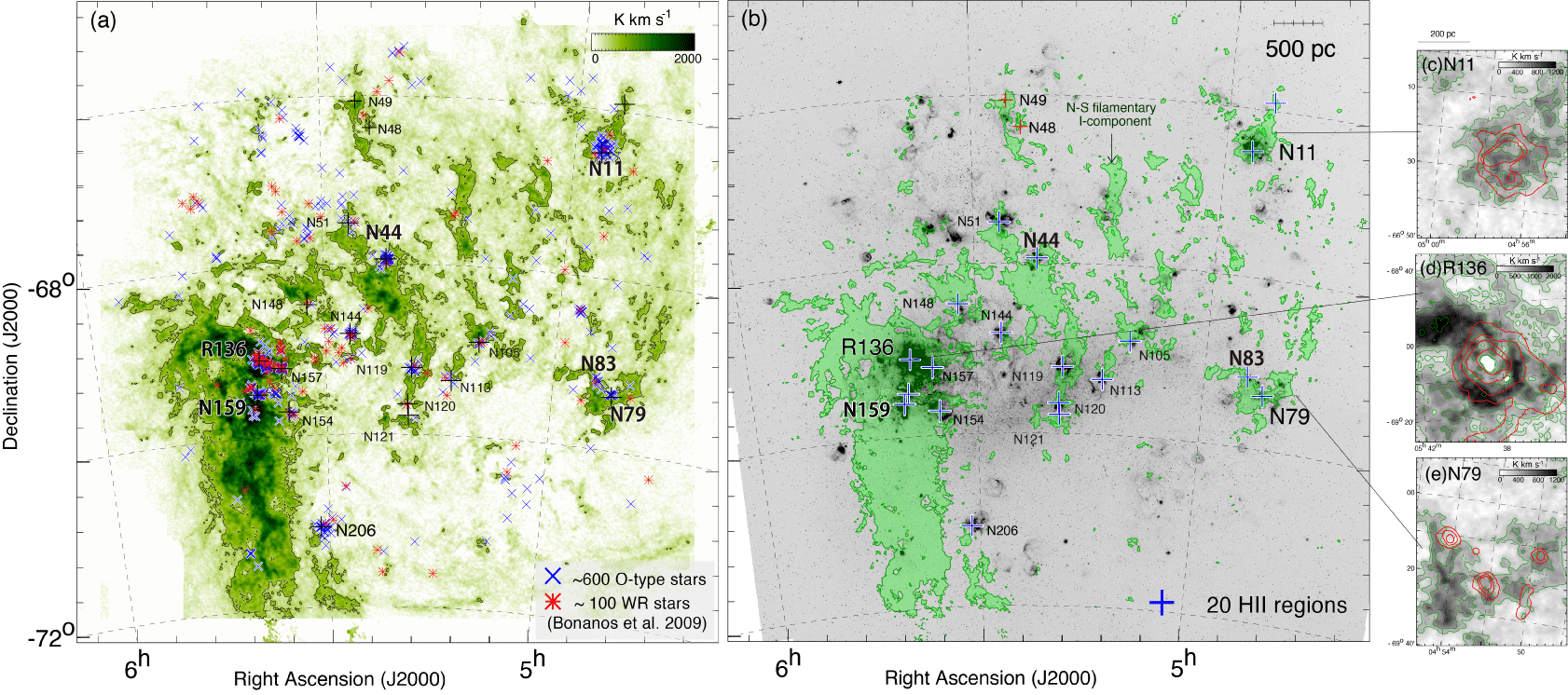
Figure 5: (a) The Hi integrated intensity map of the I-component. The red asterisks and blue crosses indicate WR stars and O-type stars (Bonanos et al. 2009), respectively. (b) The Hi integrated intensity map of the I-component by contours superposed on H$\alpha$ image. The symbols are the same as in Figure 1. The contour level of Hi is 300 K km s${}^{-1}$. (c) (d) (e) show enlarged view toward N11, R136, and N79, respectively. Images and green contours show Hi distributions. Red contours show H$\alpha$ image. The contour levels of Hi are 50, 150, and 250 K km s${}^{-1}$. The contour levels of H$\alpha$ are 150, 300, 450, and 600 R. Detailed velocity channel maps are shown in Appendix 2.

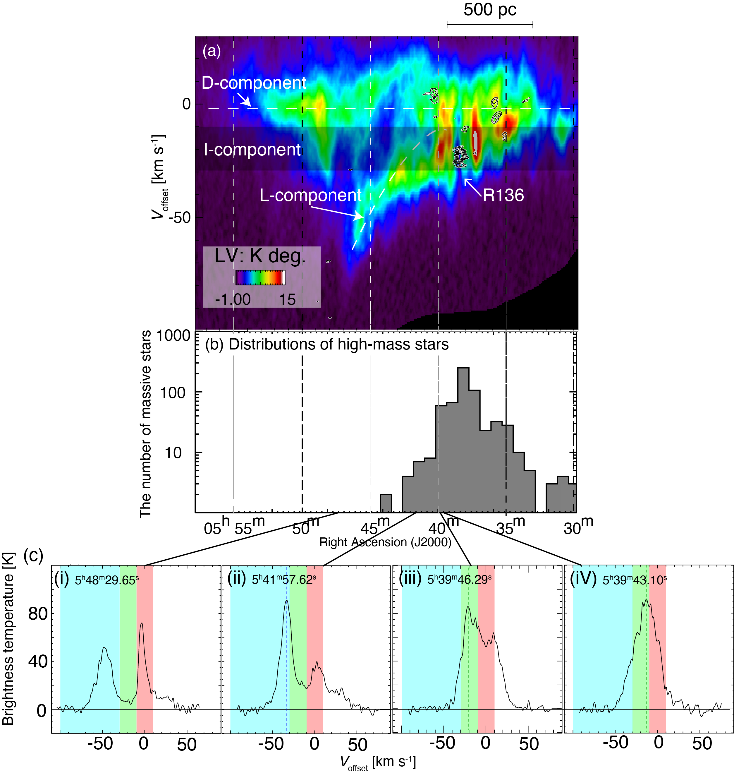
Figure 9: (a) Right Ascension–velocity diagram toward the northern part of Hi Ridge. Integration range in Declination is from $-$69.01 deg. to $-$68.79deg. at R.A. of 6h 00m 00s as shown by two black lines in Figure 7(b). The black contours indicate ${}^{12}$CO ($J$=1–0). The contour levels are 0.0133, 0.0171, 0.0209, 0.0247, and 0.0285 K deg. (b) Histogram of the number of the high-mass stars of the Hi Ridge in the same field as in Figure 7(c). The horizontal and vertical axes are R.A. and the number of massive stars located within each R.A. bin, respectively. (c) Typical spectra of Hi at the position of (i) (R.A., Dec.)=(5${}^{h}$48${}^{m}$29.65${}^{s}$,-69${}^{d}$23’3.49”), (ii) (R.A., Dec.)=(5${}^{h}$41${}^{m}$57.62${}^{s}$,-69${}^{d}$09’26.54”), (iii) (R.A., Dec.)=(5${}^{h}$39${}^{m}$46.29${}^{s}$,-69${}^{d}$09’42.95”), and (iV) (R.A., Dec.)=(5${}^{h}$39${}^{m}$43.10${}^{s}$,-69${}^{d}$00’20.42”). Blue, green, and red shaded ranges are $V_{\rm offset}$=$-101.1$–$-$30.5 km s${}^{-1}$ (the L-component), $V_{\rm offset}$=$-30.5$–$-$10.4 km s${}^{-1}$ (the I-component), and $V_{\rm offset}$=$-10.4$–$-$9.7 km s${}^{-1}$ (the D-component), respectively.

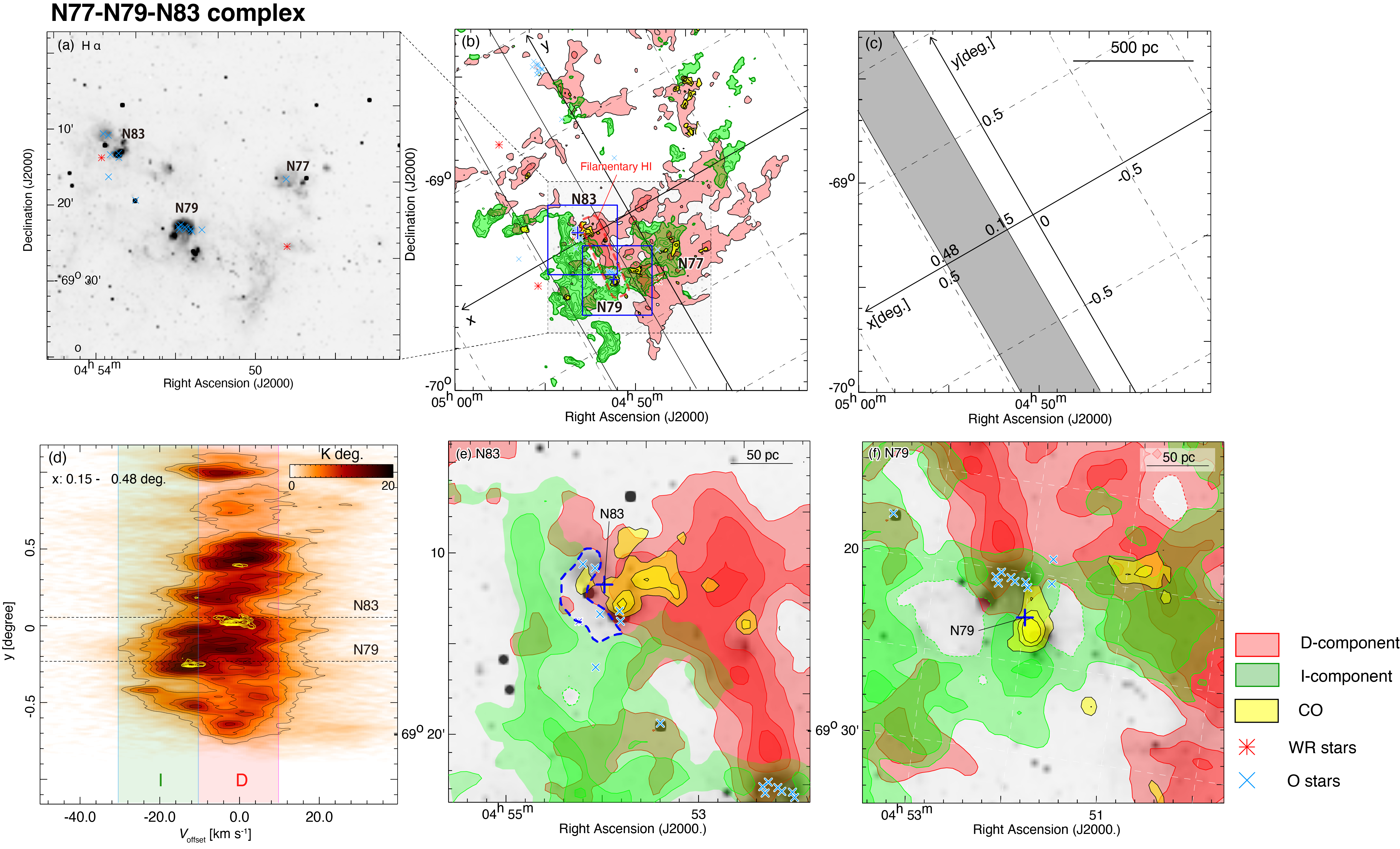
Figure 12: (a) H$\alpha$ image obtained by the Magellanic Cloud Emission-Line Survey (MCELS; Smith & MCELS Team 1999) toward N77-N79-N83 complex shown by black dashed box in (b). (b) Hi integrated intensity map of the I-component by green contours superposed on the D-component in red. The lowest contour level and intervals are 350 K km s${}^{-1}$ and 100 K km s${}^{-1}$. The yellow shaded and contours indicate the total integrated intensity map of CO ($>$ 1.5 $\sigma$ (3.89 K km s${}^{-1}$); Wong et al. 2011). The contour levels are 3.89, 7.78, and 12.97 K km s${}^{-1}$. The red cross, red asterisks, and blue crosses of (a), (b), (e), and (f) indicate the position of N11 (Henize 1956), WR stars, and O-type stars (Bonanos et al. 2009), respectively. (c) XY coordinate used for making position–velocity diagram shown (d). The center of the map at (R.A., Dec.)=(4${}^{h}$51${}^{m}$33.4${}^{s}$, $-$69${}^{d}$01${}^{m}$49.3${}^{s}$) is set as the origin of XY coordinate, and the position angle of the Y axis is $-$30 deg. (d) Position–velocity diagram of Hi overlaid with the CO contours in yellow toward N79. The integration range in X is from 0.15 deg. to 0.48 deg. The lowest contour level and intervals are 2.5 K deg. and 2.0 K deg. for Hi and 0.0368 K deg. and 0.0123 K deg. for CO. The positions of N83 and N79 are indicated by the dashed horizontal lines. (e) (f) are close-up images of (b) toward N83 and N79, respectively. The regions are shown by blue boxes in (b)

To quantify the spatial correlation between the O/WR stars and the I-component, we present a histogram of the integrated intensity of the I-component (hereafter, $W_{\rm HI}$ (I)) at the positions of 697 O/WR stars cataloged by 2009AJ....138.1003B as shown in Figure 6. This figure indicates that $\sim$50% of the O/WR stars are located at positions where $W_{\rm HI}$ (I) $>$ 300 K km s${}^{-1}$ (green histogram of Figure 6(a)). This correlation cannot be due to chance coincidence, because the characteristics of the histogram are significantly different from what is expected for the case of a purely random distribution, which is shown by the grey histogram in Figure 6(a). The Hi intensity depressions inspected above in the R136, N11, and N77-N79-N83 complex suggest that $W_{\rm HI}$ is probably decreased by the stellar feedback toward the Hii regions from the initial value before the star formation. For the depressions of $W_{\rm HI}$ distribution, which have radii around 50 pc in Figure 5, we corrected the value of $W_{\rm HI}$(I) for the feedback effects if more than one pixel has $W_{\rm HI}$ (I) smaller than 300 K km s${}^{-1}$ i) and H$\alpha$ emission higher than 500 deci Rayleigh (dR) ii). 50 pc is a radius expected for an ionized cavity by an O star in 10 Myr when the velocity of the ionization front is assumed to be 5 km s${}^{-1}$ (e.g., 2018ApJ...859..166F). In the correction, we replace $W_{\rm HI}$ toward the star with the highest value of $W_{\rm HI}$(I) within 50 pc of the star. This method is not so strict, but we find that it is helpful to fill the obvious Hi depressions. Figure 6(b), the histogram corrected for the Hi depression, indicates that 519/697 (74 %) of the O/WR stars are located at positions where $W_{\rm HI}$(I) $>$ 300 K km s${}^{-1}$. The blue histogram of Figure 6(b)) is different from the random case (grey) and becomes more significant than in Figure 6(a) without correction. We shall discuss the possible implications of the correlation between the O/WR stars and the supergiant shells in Section 5. Figures 7–12 show detailed Hi data of the Hi Ridge, N11, and N77-N79-N83 complex regions. We defer complete discussion on these figures in Section 5 by considering the new numerical simulations presented in Section 4.

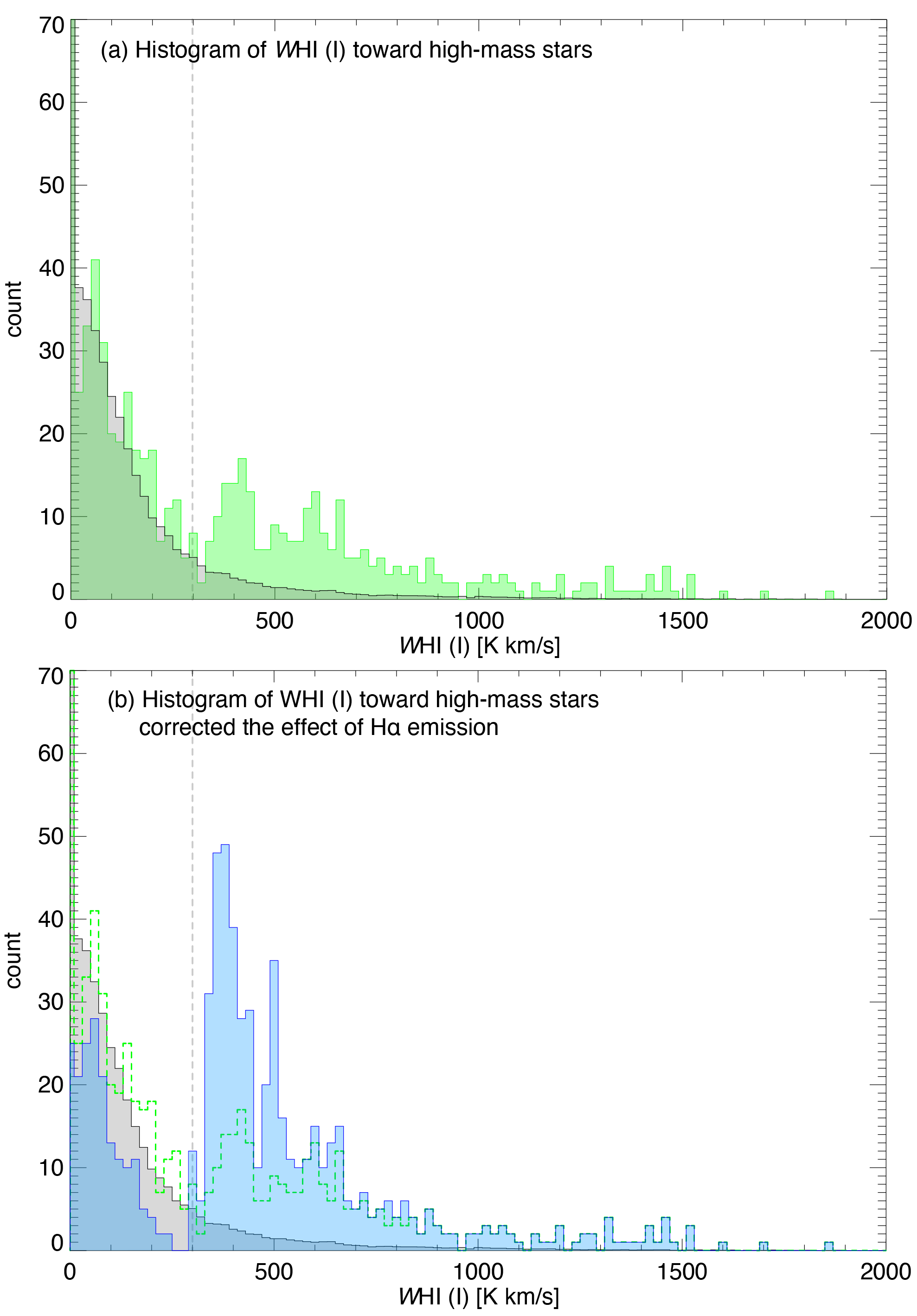
Figure 6: (a) Histograms of integrated intensity of the I-component ($W_{\rm HI}$ (I)) at the positions of 697 O/WR stars cataloged by Bonanos et al. (2009) shown in green. Grey histogram shows the distribution expected if the same number of high-mass stars are distributed at random over the whole LMC. (b) Green and grey histograms are the same as in (a). The blue histogram in (b) shows the distribution corrected for the effect of local ionization by high-mass stars. For the detailed method see section 3.3.The black vertical dashed lines indicate the threshold of ionization correction, which is set at 300 K km s${}^{-1}$

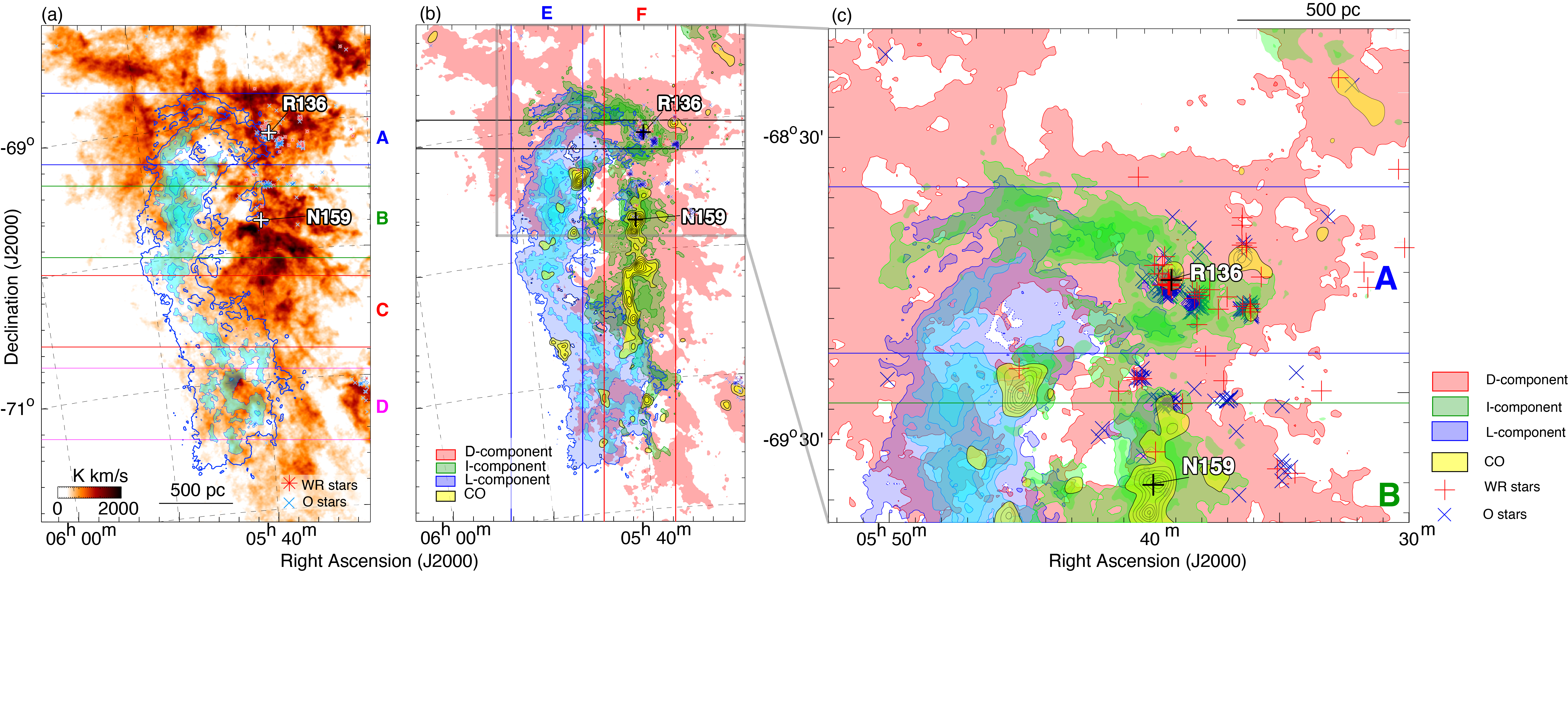
Figure 7: (a) Intensity map of Hi consisting of the L- and D-components in the Hi Ridge. The intensity map of the L-component by blue contours superposed on the D-component (orange image). The contour levels are 500, 800, 1000, 1200, 1400, 1600, 1800, and 1900 K km s${}^{-1}$. Red asterisks and light blue crosses indicate WR stars and O-type stars (Bonanos et al. 2009), respectively. The line A, line B, line C, and line D show the range in Declination where Figure 7a, 7b, 7c, 7d were made, respectively. (b) Intensity map of Hi consisting of the three velocity components (the L-, I-, and D-components) in the Hi Ridge.The red shaded area indicates the D-component where integrated intensity is larger than 500 K km s${}^{-1}$. The intensity map of the L-component by blue shaded areas and contours. The contour levels are the same as in (a). The green shaded area and contours indicate the I-component where integrated intensity is larger than 800 K km s${}^{-1}$. The contour levels are 800, 1200, 1600, and 2000 K km s${}^{-1}$. The yellow shaded area and black contours indicate the distributions of ${}^{12}$CO($J$=1–0) obtained with the NANTEN telescope. The integration velocity range is $V_{\rm offset}$=$-101.1$–9.7 km s${}^{-1}$. The lowest contour level and intervals are 1.48 K km s${}^{-1}$ (1.5 $\sigma$). Line E and line F show the range in R.A. where Figure 7e and 7f were made, respectively. The two horizontal black lines show the range in Dec. where Figure 9a was made. (c) An enlarged view of the northern part the Hi Ridge. The red crosses and blue crosses indicate WR stars and O-type stars (Bonanos et al. 2009), respectively.

4 Discussion

4.1 HI collision and star formation

4.1.1 The HI Ridge region

Paper I argued that the collision between the L- and D-components in the Hi Ridge compressed the gas to form R136 and nearby high-mass stars in the compressed layer. The metallicity was derived to be about 0.2 $Z_{\odot}$ in the region and was interpreted as a result of low metallicity gas injection from the SMC (Paper I). In the following, we explore a comprehensive picture of the triggered star formation by using position-velocity diagrams covering most of the Hi Ridge, allowing us to derive more details than in Paper I. To examine the detailed velocity structure and spatial distribution, we divided the Hi Ridge region into Lines A to F and conducted analyses. Lines A to F are all set to the same width for comparability. A to D cover the Hi Ridge region from north to south at equal intervals. Lines E and F are created to cover regions with strong L-component and strong I-component, respectively.

Complementary distribution

Figure 7(a) shows spatial distributions of the L- and D-components toward the Hi Ridge region. We recognize that the D-component shows intensity depression toward the dense part of the L-component in Zones A and B in Figure7(a) at Dec. $\sim$$-$70d–$-$69.5 d, which corresponds to the complementary distribution between the L-component and the D-component (Paper I). The complementary distribution in the north showed a displacement of 260 pc in a position angle of 45 degrees and was interpreted as due to the motion of the L-component relative to the D-component from the northwest to the southeast (Paper I). Such a displacement is a common signature in colliding clouds (2018ApJ...859..166F). Toward Zones C and D in the south, the L- and D-components significantly overlap, and the complementary distribution is less clear. In contrast, some parts of the distribution may be interpreted to be complementary (Paper I).

Figure 7(b) overlays the I-component on the L- and D-components. Figure 7c is an enlarged view of the northern Hi Ridge. The I-component is distributed mainly in the west and north of the L-component and is overlapped with the D-component. The L-component is associated with the CO-Arc in Zone E. The I-component is associated with the CO Molecular Ridge in Zone F. We recognize that high-mass star formation is active in the north of the Molecular Ridge at Dec.$>$$-$70d (Zones A–B), where R136, N159 and the other Hii regions as well as the giant molecular clouds are distributed. The distribution of the O/WR stars shows good correspondence with the I-component particularly in the west of R136 (Figure 7(c)). On the other hand, in the CO Arc and the south of the Molecular Ridge at Dec.$<$$-$70d (Zones C–D), we find no active high-mass star formation in the giant molecular clouds.

E-W and N-S distributions of the HI components; details of merging

In colliding flows, we expect the merging of the two velocity components, another feature characteristic of the collision. We explore details of the collisional merging in the Hi Ridge. Figures 8 a–d show R.A.–velocity diagrams of Hi and CO in Zones A–D (Figure 7a).

From Figures 8a–d, the P–V diagram shows a velocity gradient ranging from $-$50 km s${}^{-1}$ to 0 km s${}^{-1}$ over 500 pc from east to west. Thus, in Zones A–C, Hi gas shows a velocity gradient of $\sim$50 km s${}^{-1}$/500 pc = 0.1 km s${}^{-1}$ pc${}^{-1}$ in R.A. and seems to merge with the D-component in the west at R.A.= 5${}^{h}$ 35${}^{m}$–45${}^{m}$ along with the broad bridge features between the L- and D-components as shown in Figures 8a–c. We find a trend that the merging between the I- and L-components is more developed in the west of the L-component along the Molecular Ridge than in the east along the CO Arc. The velocity of the D-component is flattened at $V_{\rm offset}$ = 0, subtracting the rotation of the galaxy (Paper II). On the other hand, the velocity of the L-component varies with the right ascension position. Regardless of which figure (Figures 8a–d) is consulted, around 5${}^{\rm h}$50${}^{\rm m}$, the velocity is consistently in the range of $-$50 to $-$60 km s${}^{-1}$. The velocity gradient of the L-component is a natural outcome of the collisional deceleration. It suggests that the collisional interaction is taking place over a large extent of the L-component (Paper I). The I-component is a result of the deceleration and is distributed between the L- and D-components at R.A. =5${}^{h}$ 35${}^{m}$–45${}^{m}$ in Figures 8a–d.

Figure 8e shows a Dec.–velocity diagram in Zone E which includes most of the CO Arc. This clearly shows the L- and D-components as well as the several bridge features between them at Dec.$<$$-$69 d. In the region, the I-component is insignificant except for the northern end at Dec.$\sim$$-$69d., where the I component becomes enhanced, and the L-component is weak. This indicates significant merging of the two components into the I-components only at Dec.$\sim$$-$69d. It is also evident that the CO clouds in the CO Arc are all associated with the L-component.

Figure 8f shows a Dec.–velocity diagram in Zone F. We find that the I-component prevails at Dec.$>$ $-$70.5d, where the Molecular Ridge is distributed. Toward the I-component, the L-component is very weak. At Dec.$<$$-$70.5d, the I-component is weaker than at Dec.$>$ $-$70.5d and seems connected with the L- and D-components forming a few bridge features at Dec.$\sim$$-$70.5d–$-$71.5d. At Dec. of N159, the maximum Hi column density is 1.7$\times$10${}^{21}$ cm${}^{-2}$ in Zone E, while that in Zone F is more than doubled to 4$\times$10${}^{21}$ cm${}^{-2}$. This increase is consistent with the fact that the L- and D-components are merging toward the Molecular Ridge. We also note a moderate decrease in the Hi column density of the I-component from the north to the south; the Hi column density is $\sim$4$\times$10${}^{21}$ cm${}^{-2}$ in Zones A–B, $\sim$3$\times$10${}^{21}$ cm${}^{-2}$ in Zone C, and $\sim$2.5$\times$10${}^{21}$ cm${}^{-2}$ in Zone D, suggesting a N–S gradient in column density.

Figure 9 focuses on the horizontal Zone toward the R136 region, indicated by two black lines in Figure 7b. The number of O/WR stars is plotted in Figure 9b, which peaked toward R136 and is enhanced in an R.A. range from 5${}^{h}$35${}^{m}$ to 5${}^{h}$40${}^{m}$. These O/WR stars are possible outcomes of the triggered star formation by the same event that formed R136 as previously suggested (Paper I). In Figure 9c, the four Hi profiles along the Zone show details of merging, which forms the I-component from the east to the west. Further details of the triggering process will be clarified by investigating the stellar properties, which are beyond the scope of the present paper.

Physics of the merging of the HI components

The above shows that the merging process seems different between the CO Arc and the Molecular Ridge. In the Molecular Ridge, the collision of the L- and D-components leads to merging to form the I-component and the Molecular Ridge, whereas it does not lead to merging in the CO Arc as shown by no intense I-component toward the CO Arc. We explore how the difference is explained below.

A possible scenario i) is that the collision toward the CO Arc is in the early stage, and the merging of the two components has not yet occurred significantly, whereas the two components collided heavily toward the present Molecular Ridge and developed the I-component. We suggest that the Molecular Ridge was formed by the Hi collision in the I-component in less than 10 Myr, while the molecular gas in the CO Arc was pre-existent before the collision. This is possible if the initial separation between the L-component and the D-component is more prominent toward the CO Arc than toward the Molecular Ridge. We suggest a tilt of the L-component in the east to west relative to the D-component explains such a scenario if we assume that the L-component is a flat plane-like cloud. An alternative scenario ii) is that the L-component of the CO Arc region has significantly higher Hi column density than that of the D-component. In contrast, the column density was similar between the L- and D-components toward the Molecular Ridge. In scenario ii), the L-component in the CO Arc experiences minimal deceleration even upon collision. Because the CO Arc is located toward the edge of the LMC disk, the lower column density of the D-component is reasonable. At Dec.$\sim$$-$70.3d.–$-$69.3d the column density of the L-component, which is associated with the giant molecular clouds, is higher than that of the D-component (Figure 8e) and may support scenario ii). In summary, we find that the two scenarios are viable explanations. They are not exclusive and both may be working.

Overall high-mass star formation in the HI Ridge

The formation of the high-mass stars and the GMCs is active only in the northern half of the Hi Ridge (Figure 7b); $\sim$400 O/WR stars are concentrated in an area of $\sim$500 pc $\times$ $\sim$500 pc in the northwest of the Hi Ridge at Dec.$>$$-$70.8 d, and the GMCs are distributed at Dec.$>$ $-$70.0 d. On the other hand, the southern half of the Hi Ridge is quiescent in high-mass star formation. The morphology that the absorption in the soft X-rays independently supports the L-component with a tilt located in front of the LMC disk (Sasaki et al. 2022; Knies et al. 2021) and in the near infrared extinction (Furuta et al. 2019, 2021). It is worth mentioning that the soft X-rays are likely emitted from the gas between the Molecular Ridge and the CO Arc heated by the gas collision at $\sim$100 km s${}^{-1}$ (Knies et al. 2021) as is consistent with the colliding Hi flows. This direction of the falling motion of the L-component is further supported by the ALMA observations of colliding CO clouds in N159 (Fukui et al. 2019; Tokuda et al. 2019; 2022).

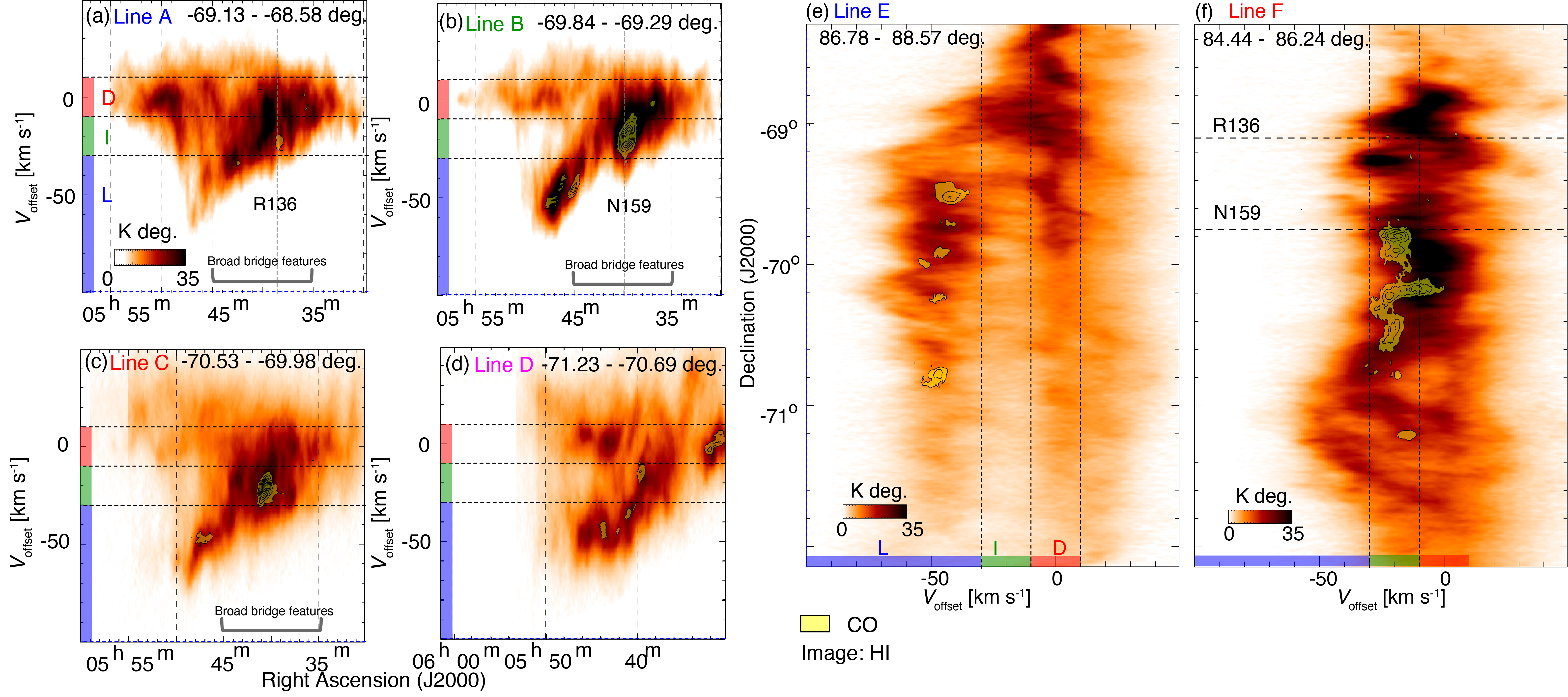
Figure 8: (a)–(b) Right Ascension–velocity diagrams of Hi by image overlaid with the CO by yellow contours along lines A, B, C, and D in unit of K degree. The integration is in Dec. over the range from $-$69.13 to $-$68.58 deg. for (a), $-$69.84 to $-$69.29 deg. for (b), $-$70.50 to $-$69.95 deg. for (c), and $-$71.32 to $-$70.77 deg. for (d). The lowest contour level and intervals are 0.0241 K deg. and 0.0241 K deg., respectively. (e)(f) Declination–velocity diagram of Hi by image overlaid with the CO by yellow contours along Lines E and F in unit of K degree. The integration ranges in Right Ascension are from 86.78 to 88.57 degree for (e) and 84.44 to 86.24 degree for (f). The lowest contour level and intervals are 0.0241 K deg. and 0.0241 K deg., respectively.

These observational trends obtained with Hi, CO, and X-ray suggest that the collisional compression propagates from the north to the south, and the active high-mass star formation only in the north may be explained by the propagating time-dependent star formation in a timescale of $\sim$10 Myr. Figure 10 shows the 3D geometry of the collision toward the Hi Ridge. The time scale is roughly consistent with the evolutionary stage of giant molecular clouds (GMCs) of the Hi Ridge region (1999PASJ...51..745F; 2009ApJS..184....1K, see also Kawamura 2010). In addition, it is interesting to note that the GMC evolutionary stages show a north-south sequence of star formation. In the northern part, most of the molecular gas around R136 is classified as Type III, a molecular cloud associated with active cluster formation and Hii regions. In the southern part of R136 including N159, there are many Type II GMCs, which are in the younger stage and are associated only with Hii regions. In the more southern region, the youngest Type I GMCs without associated Hii regions are dominant. The time scales of Type I, Type II, and Type III are estimated to be 6 Myr, 13 Myr, and 7 Myr, respectively, by 2009ApJS..184....1K, which are similar to the time scale of the collision. Thus, the north-south sequence of star formation in the Hi Ridge region may be explained by the three-dimensional structure of the collision we proposed.

We need to consider the smaller-scale processes to deepen our understanding of the high-mass star formation in the Hi Ridge. In particular, the recent ALMA results revealed that the high-mass star formations in the ”peacock-shaped clouds” in N159E and N159W-S are triggered by a pc-scale falling cloud colliding with extended gas (2019ApJ...886...14F; 2019ApJ...886...15T). In addition, such a collision was numerically simulated by 2018PASJ...70S..53I and it was shown that the collisional compression reproduces filamentary conical dense gas distribution. Follow-up ALMA observations revealed that N159W-N also shows the CO distribution consistent with the simulations of Inoue et al. (2018). It is notable that the direction of these falling clouds is parallel to the direction derived from the kpc-scale displacement in the NW–SE direction. (2023ApJ...955...52T). These results suggest that the interaction of falling clouds with the disk, as a consequence of the tidal interaction, is a vital process to form high-mass stars. We present a detailed picture that the colliding Hi flows consist of small dense (10–100 cm${}^{-3}$) Hi clumps of pc-scale and the clumps trigger high-mass star formation at individual spots separated by tens of pc over a kpc scale. Future ALMA observations will be crucial to broaden the application of the scenario to the rest of the LMC where high-mass star formation is occurring.

4.1.2 The Diffuse L-component

In Paper II, the colliding Hi flows with low metallicity are found to trigger the high-mass star formation in N44. N44 is part of the Diffuse L-component, and it is likely that the colliding Hi flows include the metal-poor gas injected from the SMC, as shown by the dust-to-gas ratio in Paper II.

The Hi position–velocity diagrams in Figures LABEL:fig21 (a) to (k) of Appendix 4 show that the L- and D-components are connected in a velocity space toward N44.

The Diffuse L-component has an approximate size of 1.5 kpc $\times$1.5 kpc in R.A. and Dec. with a triangle shape whose vertex is directed toward the south (Figure 3). The I-component toward the Diffuse L-component is divided into four features; they are the southeastern part, including N44, N51, and N144, the southwestern part, including N105 and N113, the southern part, including N119, N120, and N121, and the northern filamentary part with a few small Hii regions and no major Hii regions (Figure 5b).

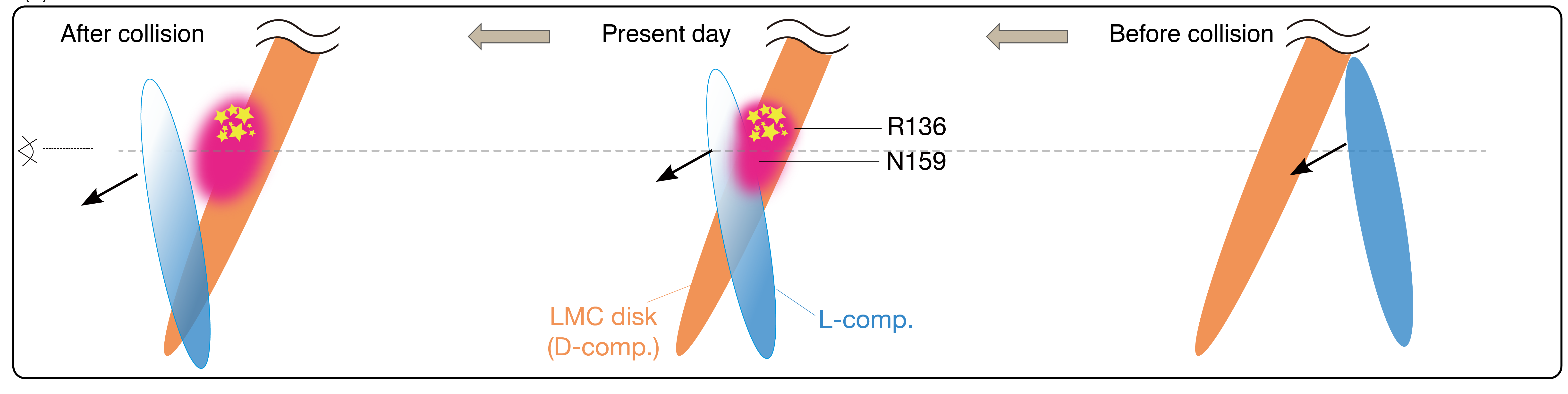
Figure 10: Schematic view of the collision. Orange and blue disks are the D- and L-component, respectively. The red area represents the distribution of diffuse soft X-ray (e.g., Knies, et al. 2021). The line of sight direction is from left to right. From right to left, it shows the geometry before the collision $(right)$, the present state $(center)$, and the geometry after the collision $(left)$.

We interpret that the I-component was formed by the southward motion mainly at the southern edge of the L-component by the collisional compression, which explains that most of the I-component is distributed on the south side of the L-component. Moreover, the first-moment map shows that the Diffuse L-component is decelerated at the southern edge, as illustrated in Figure 4(a). It is possible that the Diffuse L- and D-components are merging to form the I-component in the south of the Diffuse L-component. On the other hand, the northern part of the Diffuse L-component is not decelerated and the first moment is $\sim$$-$50 to $-$60 km s${}^{-1}$. There is no I-component toward this region, as shown in Figure 3, so the L-component is possibly before or at the beginning of collision with slight deceleration. Moreover, there is no significant molecular cloud/high-mass star formation, which is consistent with the idea that no significant compression by collision is yet taking place.

We suggest that in N44, the V-shaped southern part of the I-component is the strongly compressed layer that formed seven of the 20 major Hii regions. The morphology may be explained by a scale-up version of the colliding cloud of pc-scale modeled and simulated by 2018PASJ...70S..53I, which assumes that a test spherical cloud is collides with extended gas. The simulations by 2018PASJ...70S..53I show that the collision forms a compressed layer of a conical shape pointing toward the moving direction of the spherical cloud. Such conical clouds are indeed discovered in three regions of collision-induced high-mass star formation at a pc-scale in N159, i.e., N159E, N159W-S, and N159W-N (Fukui et al. 2019; Tokuda et al. 2019; 2022). These three cases are believed to be those for which Inoue et al. (2018)’s model is applicable. In the Diffuse L-component, we suggest that a kpc-scale cloud of the L-component largely collided from the north with the D-component, and the I-component of a V-shape was formed in a kpc scale. This scenario will be tested in more detail by using the new simulations and the Hi/CO observations toward the individual Hii regions in the future.

Figure 11: (a) Hi integrated intensity map of the L-component by blue shaded area ($>$ 150 K km s${}^{-1}$) superposed on the D-component by image. (b) Hi integrated intensity map of the I-component by green shaded area ($>$ 500 K km s${}^{-1}$) superposed on the D-component. The white shaded area and contours of (a) and (b) indicate the total integrated intensity map of CO ($>$ 1.5 $\sigma$ (3.89 K km s${}^{-1}$); Wong et al. 2011). The contour levels are 3.89, 7.78, and 12.97 K km s${}^{-1}$. The red cross, red asterisks, and blue crosses indicate the position of N11 (Henize 1956), WR stars, and O-type stars (Bonanos et al. 2009), respectively. (c) Position–velocity diagram of Hi by image overlaid with the CO by blue contours. The lowest contour level and interval are 1.5 K deg. and 1.0 K deg. for Hi; 3 $\sigma$ (0.024 K deg.) and 1 $\sigma$ (0.008 K deg.) for CO.The integration range in Dec. is from $-$66.61${}^{\circ}$ to $-$66.47${}^{\circ}$ shown by the black horizontal lines of (a). The red dashed perpendicular line indicates the position of N11 in the R.A.. (d) H$\alpha$ image obtained by the Magellanic Cloud Emission-Line Survey (MCELS; Smith & MCELS Team 1999) toward N11 shown by black dashed box in (a). The black circle indicates a ring morphology with a cavity of $\sim$100 pc in radius, enclosing OB association LH9 (Lucke & Hodge 1970).

The maximum column density of the L-component is $\sim$2.6$\times$10${}^{21}$ cm${}^{-2}$, while the D-component has a column density of 3.2$\times$10${}^{20}$ cm${}^{-2}$, an order of magnitude smaller than that of the Diffuse L-component at the same position. It is possible that the low column density of the D-component is a result of the collisional acceleration which shifted the D-component to the L-component.

Examining the effects of the stellar feedback in exploring high-mass star formation is important. Because the energy released by the high-mass stars is large and all the region discussed above includes 40–400 O/WR stars. By adopting typical physical parameters of the stellar feedback, we calculated the cloud mass and the kinetic energy of the L-component for velocity relative to the D-component at two assumed angles of the motion 0${}^{\circ}$and 45${}^{\circ}$ to the sightline. Table 2 lists these physical parameters in the N11 and N77-N79-N83 complex. We find that the momentum released by the stellar feedback is lower by two orders of magnitude than that required to accelerate the motion of the I-component. Furthermore, we do not find any strong enhancement of the Hi gas motion toward the O/WR stars in each of the present regions, whereas the Hi velocity components are extended spatially. This indicates gas acceleration is extended over more than a few 100 pc but is not localized toward the O/WR stars, which is not consistent with stellar feedback. The gas motion is, therefore, not likely driven by the feedback but by the large kpc-scale tidal interaction. The similar arguments on R136 and N44 in Papers I and II are consistent with the present conclusion. In the following section, we will not discuss stellar feedback as a cause of gas motion in the following, while ionization localized to the individual high-mass star formation is obviously important.

4.1.3 N11 region

The Hii region N11 was cataloged by 1956ApJS....2..315H. N11 has a ring morphology with a cavity of $\sim$100 pc in radius, enclosing OB association LH9 in the center of the cavity (Lucke & Hodge 1970). There are several bright nebulae (N11B, N11C, N11F) around LH9 as shown in the H$\alpha$ image (MCELS; Smith & MCELS Team 1999) in Figure 11. The massive compact cluster HD 32228 dominates this OB association and has an age of $\sim$3.5 Myr (1999AJ....118.1684W). LH 10 is the brightest nebula and lies north of LH 9. LH 10 is the youngest OB association with an age of about 1 Myr. Previous studies proposed that star formation in LH10 was possibly triggered by an expanding supershell blown by LH9 (e.g., 1996A&A...308..588R; 2003AJ....125.1940B; 2006AJ....132.2653H; 2019A&A...628A..96C). 1996A&A...308..588R conducted a detailed analysis of the kinematics of H$\alpha$ emission and determined an expansion velocity of 45 km s${}^{-1}$ for the central cavity. The authors suggested that a dynamical age of expansion is 2.5$\times$10${}^{6}$ years, and a possible product of the explosion includes three SNe and shock-induced star formation.

The present Hi data reveal features that were not considered previously. Figure 11a shows the L-component and the D-component, and Figure 11c shows the I-component and the D-component. Figure 11d presents a position-velocity diagram in the Zone shown by two black straight lines in Figure 11a. The I-component and the D-component show complementary distribution. The I-component fits the cavity of the D-component toward the center of the H$\alpha$ cavity. In addition, there are O stars, emission nebulae, and GMCs outside the cavity of N11, some of which overlap with the I-component. Further, the position-velocity diagram shows that the I-component and D-component are merged, forming a V-shaped distribution, another signature of a cloud-cloud collision along with the complementary distribution (2021PASJ...73S...1F). The L-component here is a minor feature and we interpret it as part of the I-component.

Based on these data, we propose a colliding flow scenario as a trigger of N11, where a single spherical Hi cloud of $\sim$100pc radius collided with the D-component. The spherical cloud accompanies a few extended components of 100–200 pc length outside a 100 pc radius, which is observed as the present I-component. We assume that the collisional interaction has a path length of $\sim$100 pc, the same as the approximate radius of the high-mass star distribution in Figure 11. Then, the collision time scale is roughly estimated to be 100 pc / 30 km/s $\sim$ 3 Myr, which is consistent with an age of LH9 ( 3.5 Myr; Walborn et al. 1999). In the collision scenario, the age sequence between LH9 and the rest of the OB associated is ascribed to the different epochs of the collision due to the Hi morphology. First, a collision triggered star formation in LH9 at the center of N11. Then, the collision proceeded outward in a shell-like distribution and triggered the formation of the other younger OB associations in the periphery, including LH11, LH10, and LH13 in the last few Myr. Additionally, LH13 was formed by the collision between the extended I-component and the D-component. The I-component associated with LH9 is already ionized mostly (Figure 11c). In the previous expansion-shell trigger, the first OB association was given as the initial condition. This scenario explains the formation of the first OB association and the other OB associations consistently by the collisional compression.

Table 2: Comparison of gas momentum and stellar wind momentum

Object	$M$Hi	$M_{\rm CO}$	$M$Hi + $M_{\rm CO}$	Momentum	$\#$ of	$\#$ of	Momentum
	(I + D)	(I + D)		of gas	O-stars	WR stars	of stellar wind
	[10${}^{6}M_{\odot}$]	[10${}^{5}M_{\odot}$]	[10${}^{6}M_{\odot}$]	[10${}^{5}M_{\odot}$ km s${}^{-1}$]			[10${}^{5}M_{\odot}$ km s${}^{-1}$]
(1)	(2)	(3)	(4)	(5)	(6)	(7)	(8)
N11	2.3	4.5	2.8	840	67	2	1.4
N79	2.6	3.7	3.0	900	17	2	0.4

Column (1): Object name. Column (2): Hi mass of the D- and I-component within a radius of 200 pc. Column (3): CO mass of the D- and I-component within the radius of 200 pc. Column (4): Total mass of Hi and CO. Column (5): Momentum of gas. Column (6): Number of O stars. Column (7): Number of WR stars. Column (8): Total momentum of stellar wind of O/WR stars.
We assumed that expansion velocity of gas is 30 km s${}^{-1}$, which is velocity difference between the L- and I-components. We used momentum of stellar wind of O/WR stars calculated by mass loss rate and wind velocity (Abbott et al. 1982; Kudritzki & Puls 2000). $D_{\rm mom}$ = $m_{\rm loss}$$\times$$v$$\times$$t$($m_{\rm loss}$: mass loss rate, $v$: wind velocity, $t$: wind duration time). O stars: $D_{\rm mom}$$\sim$2000 [$M_{\odot}$ km s${}^{-1}$] ($m_{\rm loss}$$\sim$10${}^{-6}$$M_{\odot}$ yr${}^{-1}$; $v$$\sim$2000 km s${}^{-1}$; $t$$\sim$10${}^{6}$ yr). WR stars: $D_{\rm mom}$$\sim$2500 [$M_{\odot}$ km s${}^{-1}$] ($m_{\rm loss}$$\sim$3$\times$10${}^{-5}$$M_{\odot}$ yr${}^{-1}$; $v$$\sim$2500 km s${}^{-1}$; $t$$\sim$3$\times$10${}^{5}$ yr).