Abstract

We investigate scalarized black holes in the Einstein-minimally coupled scalar theory with a negative potential $V(\phi)=-\alpha^{2}\phi^{6}$. The tachyonic instability is absent from analyzing the linearized scalar equation, which could not allow for spontaneous scalarization. However, we obtain the black hole solutions with scalar hair by solving three full equations because this scalar potential violates the weak energy condition. This shows clearly that scalarized black holes can be obtained without introducing a non-minimal scalar coupling term. We perform the stability analysis for scalarized black holes by adopting radial perturbations, implying that all scalarized black holes belonging to a single branch are unstable.

1 Introduction

The no-hair theorem in general relativity (GR) prevents the existence of asymptotically flat black hole solutions with scalar hair except the mass $M$, angular momentum $J$, and charge $Q$ of the black hole [1, 2, 3]. This is based on the Einstein-minimally coupled scalar theory [4].

If one introduces a conformally coupled scalar (Einstein-conformally coupled scalar theory), it gave us the BBMB black holes with a conformal scalar hair, indicating an evasion of no-hair theorem [5, 6]. In this case, however, the conformal scalar hair blows up at the horizon and these black holes are unstable under linear perturbations.

Recently, it is well known that infinite branches of scalarized (charged) black holes were obtained numerically from the Einstein-Gauss-Bonnet-scalar theory [7, 8, 9, 10] (Einstein-Maxwell-scalar theory [11]) through the non-minimal coupling of a scalar function to the Gauss-Bonnet term (Maxwell term). In these linearized theories, the tachyonic instability of $s(l=0)$-scalar mode propagating around the GR black holes indicates the onset of spontaneous scalarization. This arose from either the negative Gauss-Bonnet coupling term ($-48\lambda^{2}M^{2}/r^{6}$) or the negative Maxwell coupling term($-2\alpha Q^{2}/r^{4}$) where $\lambda^{2}$ and $\alpha$ are positive scalar coupling parameters. These negative coupling terms induce actually potential wells near the horizon and as coupling parameters increase, leading to tachyonic instabilities. Furthermore, the linearized static scalar equation has played an important role in obtaining scalar clouds (bound states). Requiring an asymptotically vanishing scalar, the condition for obtaining a smooth scalar selects a discrete set of the bifurcation points for scalarized solutions: $M/\lambda=\{0.587,0.226,0.140,\cdots\}~{}(\alpha(q=0.7)=\{8.019,40.84,99.89,\cdots\})$ for the Gauss-Bonnet term [12] (as well as the Maxwell term [13]). They have admitted scalar hairy black holes in the full theory. Actually, it has induced infinite branches of scalarized [charged] black holes: $n=0(0<M/\lambda<0.587),1(0<M/\lambda<0.226),2(0<M/\lambda<0.140),\cdots[n=0(\alpha>8.019),n=1(\alpha>40.84),n=2(\alpha>99.89),\cdots]$.

However, it turned out that the $n=0$ branch of scalarized (charged) black holes are stable against radial perturbations, whereas all other branches of $n\not=0$ are unstable [14]. This implies that the $n=0$ branch of scalarized (charged) black holes could survive for further implications of scalarized black holes. In this direction, the dynamics of scalarized black holes and binary mergers were addressed in the Einstein-Gauss-Bonnet-scalar theory [15, 16, 17, 18, 19, 20, 21]. Furthermore, the photon spheres and observational appearance of scalarized black holes are investigated in the Einstein-Maxwell-scalar theory [22, 23, 24, 25, 26, 27, 28, 29].

In this work, we focus on introducing a newly simple mechanism to obtain scalarized black holes from a negative potential term $V(\phi)=-\alpha^{2}\phi^{6}<0$ in the Einstein-minimally coupled scalar theory without depending on any scalar coupling terms. Hence, the tachyonic instability is absent. In this case, we obtain a single branch of scalarized black holes in Einstein-minimally coupled scalar theory. Carrying out stability analysis for scalarized black holes by adopting radial perturbations, we find that all scalarized black holes belonging to a single branch are unstable. This implies that even though one obtains easily scalarized black hole from the simplest scalar-tensor action, they are hard to survive for further implications.

The present work is inspired from the hairy black hole solutions in Einstein-Weyl-massive conformally coupled scalar theory where the tachyonic scalar mass has played an important role in obtaining scalar hairy black holes [30]. In the absence of tachyonic mass term ($-m^{2}\phi^{2}$), we have obtained the non-BBMB black hole solution in the new massive conformal gravity [31]. Also, this work is motivated strongly from finding scalarized black hole in the Einstein-minimally coupled scalar theory with an asymmetric scalar potential which contains a negative region, indicating a violation of the weak energy condition (WEC) [32, 33, 34, 35]. Besides, the asymmetric potential has also been employed to construct the fermionic stars [36, 37]. A symmetric potential of $V(\phi)=\mu\phi^{2}-\Lambda\phi^{4}$ violating the WEC was also introduced to obtain the scalarized black holes [38], which can be smoothly connected with the counterpart gravitating scalaron in the small horizon limit [39]. Note that this gravitating scalaron can possess the positive Arnowitt-Deser-Misner (ADM) mass but previously another type of gravitating scalaron with negative ADM mass was constructed by employing the Higgs-like potential with a phantom field [40], hence this demonstrates that the use of phantom field can be avoided for the construction of gravitating scalaron. The no-hair theorem suggests that asymptotically flat black holes with scalar hair do not exist if a scalar matter satisfies the WEC [41]. Hence, if the WEC for a scalar matter is violated, scalarized black holes could be found from the Einstein-minimally coupled scalar theory. As far as we know, our model corresponds to a simplest model which violates the WEC because of a negative potential and thus, it could induce scalarized black holes without introducing a non-minimal scalar coupling term. Other types of scalarized black holes in the Einstein-minimally coupled scalar theory can be found in Ref. [42, 43, 44, 45, 46, 47, 48, 49, 50, 51, 52, 53]. Besides, recently this similar concept has been adopted to construct a traversable wormhole in the Einstein-3-form theory with the Higgs-like potential, which is sufficient to violate the null energy condition where the phantom field is no longer needed and the kinetic term still can remain the correct sign [54].

2 No tachyonic instability of Schwarzschild black hole

We start with the Einstein-minimally coupled scalar theory defined by

$$S_{\rm Es}=\frac{1}{16\pi G}\int d^{4}x\sqrt{-g}\Big{[}\frac{R}{16\pi G}-\frac{1}{2}\nabla_{\mu}\phi\nabla^{\mu}\phi-V(\phi)\Big{]},$$ (1)

where $V(\phi)$ is a negative scalar potential

$$V(\phi)=-\alpha^{2}\phi^{6}$$ (2)

with $\alpha>0$.

The Einstein equation is derived from (1) as

$$R_{\mu\nu}-\frac{1}{2}g_{\mu\nu}R = 8\pi G\Big{[}\nabla_{\mu}\phi\nabla_{\nu}\phi-g_{\mu\nu}\Big{(}\frac{1}{2}\nabla_{\alpha}\phi\nabla^{\alpha}\phi+V(\phi)\Big{)}\Big{]}.$$ (3)

On the other hand, the scalar equation is given by

$$\nabla^{2}\phi=\frac{dV(\phi)}{d\phi}.$$ (4)

Considering

$$\bar{R}_{\mu\rho\nu\sigma}\not=0,~{}~{}\bar{R}_{\mu\nu}=0,~{}~{}\bar{R}=0,~{}~{}\bar{\phi}=0,$$ (5)

Eqs. (3) and (4) imply the GR (Schwarzschild) black hole solution

$$ds^{2}_{\rm Sch}=\bar{g}_{\mu\nu}dx^{\mu}dx^{\nu}=-f(r)dt^{2}+\frac{dr^{2}}{f(r)}+r^{2}d\Omega^{2}_{2}$$ (6)

with the metric function

$$f(r)=1-\frac{r_{0}}{r}.$$ (7)

Here the event horizon appears at $r_{H}=r_{0}$. We note that $\bar{\phi}=$ const is not allowed for getting a GR black hole.

Now, let us introduce the scalar and metric perturbations around the Schwarzschild black hole

$$g_{\mu\nu}=\bar{g}_{\mu\nu}+h_{\mu\nu},~{}~{}\phi=0+\delta\phi.$$ (8)

Firstly, we consider the scalar perturbation. Considering (4), its linearized scalar equation is given by

$$\bar{\nabla}^{2}\delta\phi=0.$$ (9)

Reminding the spherically symmetric background (6), it is convenient to separate the scalar perturbation into modes

$$\delta\phi(t,r,\theta,\varphi)=e^{-i\omega t}Y_{lm}(\theta,\varphi)\frac{u(r)}{r}\,,$$ (10)

where $Y_{lm}(\theta,\varphi)$ is spherical harmonics with $-m\leq l\leq m$. Introducing a tortoise coordinate $r_{*}=r+r_{0}\ln(r/r_{0}-1)$ defined by $dr_{*}(r)=dr/f(r)$, a radial part of the wave equation leads to the Schrödinger-type equation as

$$\frac{d^{2}u}{dr_{*}^{2}}+[\omega^{2}-V_{\rm s}(r)]u(r)=0,$$ (11)

where the scalar potential $V_{\rm s}(r)$ takes the form

$$V_{\rm s}(r)=f(r)\Big{[}\frac{r_{0}}{r^{3}}+\frac{l(l+1)}{r^{2}}\Big{]},$$ (12)

which is always positive definite for any $l$ outside the horizon. Therefore, there is no tachyonic instability and the Schwarzschild black hole is stable against scalar perturbation.

Now, we briefly mention the tensor perturbation. The linearized Einstein equation around the Schwarzschild black hole is simply given by

$$\delta G_{\mu\nu}=0$$ (13)

where the linearized Einstein tensor is expressed in terms of linearized Ricci tensor and Ricci scalar as

$$\delta G_{\mu\nu} = \delta R_{\mu\nu}-\frac{1}{2}\delta R\bar{g}_{\mu\nu},$$ (14)

$$\delta R_{\mu\nu} = \frac{1}{2}\Big{(}\bar{\nabla}^{\rho}\bar{\nabla}_{\mu}h_{\nu\rho}+\bar{\nabla}^{\rho}\bar{\nabla}_{\nu}h_{\mu\rho}-\bar{\nabla}^{2}h_{\mu\nu}-\bar{\nabla}_{\mu}\bar{\nabla}_{\nu}h\Big{)},$$ (15)

$$\delta R = \bar{g}^{\mu\nu}\delta R_{\mu\nu}=\bar{\nabla}^{\mu}\bar{\nabla}^{\nu}h_{\mu\nu}-\bar{\nabla}^{2}h$$ (16)

with $h=h^{\rho}~{}_{\rho}$. Taking the trace of the linearized Einstein equation (13), one has

$$\delta R=0.$$ (17)

Plugging $\delta R=0$ into Eq. (13) leads to the linearized GR equation for the linearized Ricci tensor

$$\delta R_{\mu\nu}=0.$$ (18)

It is well known that the Schwarzschild black hole is stable against metric perturbation $h_{\mu\nu}$ in the GR  [56, 57, 58, 59]. This implies that the linearized stability analysis has no prediction on exploring scalarized black holes.

3 Scalarized black holes

Even though the Schwarzschild black hole appears stable against scalar perturbation, we may obtain scalarized black holes because the potential in (2) violates the WEC. First of all, we introduce a spherically symmetric metric to construct the scalarized black holes solutions

$$ds^{2}_{\rm Sb}=-N(r)e^{-2\sigma(r)}dt^{2}+\frac{dr^{2}}{N(r)}+r^{2}d\Omega^{2}_{2}$$ (19)

with $N(r)=1-2m(r)/r$ where $m(r)$ denotes the Misner-Sharp mass function. We note that $m(\infty)=M$, the total mass of the configuration.

Plugging Eq.(19) into (3) and (4), three differential equations for metric functions ($m,\sigma$) and scalar ($\phi$) are found as

$$m^{\prime}=2\pi Gr^{2}\left(N\phi^{\prime 2}+2V\right),\quad\sigma^{\prime}=-4\pi Gr\phi^{\prime 2},\quad\left(e^{-\sigma}r^{2}N\phi^{\prime}\right)^{\prime}=e^{-\sigma}r^{2}\frac{dV}{d\phi},$$ (20)

where the prime (^′) denotes the derivative with respect to the radial coordinate $r$.

At this stage, one needs to know the asymptotic behaviour of these functions at the horizon and the infinity to construct globally defined black hole solutions. Near the horizon ($r\simeq r_{H}$), the leading forms in the series expansion are given by

$$m(r) =\frac{r_{H}}{2}+m_{1}(r-r_{H})+O\left((r-r_{H})^{2}\right),$$ (21)

$$\sigma(r) =\sigma_{H}+\sigma_{1}(r-r_{H})+O\left((r-r_{H})^{2}\right),$$ (22)

$$\phi(r) =\phi_{H}+\phi_{H,1}(r-r_{H})+O\left((r-r_{H})^{2}\right),$$ (23)

where the coefficients are given by

$$m_{1}=4\pi Gr^{2}_{H}V(\phi_{H}),\quad\sigma_{1}=-4\pi Gr_{H}\phi^{2}_{H,1},\quad\phi_{H,1}=\frac{r_{H}V^{\prime}(\phi_{H})}{1-8\pi Gr_{H}^{2}V(\phi_{H})}.$$ (24)

Here $\sigma_{H}$ and $\phi_{H}$ are the values of $\sigma$ and $\phi$ at the horizon. We note that the denominator of $\phi_{H,1}$ should satisfy the condition of $1-8\pi Gr_{H}^{2}V(\phi_{H})\not=0$ to keep $\sigma(r)$ and $\phi(r)$ should be finite at the horizon.

Asymptotic expansions of the metric and scalar functions at infinity take the forms when imposing asymptotical flatness and a vanishing scalar as

$$m(r) =M-\frac{D^{2}}{4r}-\frac{MD^{2}}{4r^{2}}-\frac{D^{2}}{3r^{3}}\left(2D^{4}+M^{2}\right)+\mathcal{O}(r^{-4})\,,$$ (25)

$$\sigma(r) =\frac{D^{2}}{4r^{2}}+\frac{2MD^{2}}{3r^{3}}+\left(\frac{3D^{6}}{2}-\frac{D^{4}}{8}+3M^{2}D^{2}\right)\frac{1}{2r^{4}}+\mathcal{O}(r^{-5})\,,$$ (26)

$$\phi(r) =-\frac{D}{r}-\frac{DM}{r^{2}}+\left(-D^{4}+\frac{D^{2}}{12}-\frac{4M^{2}}{3}\right)\frac{D}{r^{3}}+\mathcal{O}(r^{-4})\,,$$ (27)

where $M$ and $D$ represent the ADM mass and scalar charge of the hairy black hole, respectively.

Finally, introducing three dimensionless parameters

$$r\rightarrow\frac{r}{\alpha\sqrt{8\pi G}},\quad m\rightarrow\frac{m}{\alpha\sqrt{8\pi G}}\,,$$ (28)

three equations in Eq.(20) can be solved by an ODE solver package Colsys when adapting the Newton-Raphson method to solve the boundary value problem for three coupled nonlinear differential equations [60]. We employ a compactified coordinate $x=1-r_{H}/r(x\in[0,1])$ for constructing hairy black holes in the numerics. Here, we are left with the three parameters $(\phi_{H},\sigma_{H},r_{H})$ where $\sigma_{H}$ is determined when imposing $\sigma(\infty)=0$ while $r_{H}$ could be determined when all solutions satisfy the boundary conditions. In this case, the state of a scalarized black hole depends only on $\phi_{H}$ which means that different scalarized black holes are encoded in different $\phi_{H}$. When the scalar field is zero on the horizon, the corresponding configuration is solely given by the Schwarzschild black hole. However, when the scalar field on the horizon $\phi_{H}$ is non-zero and then, one increases it, a branch of hairy black holes bifurcates and behaves quite differently from the Schwarzschild black hole. To represent this behavior, we introduce reduced area $a_{H}$ and reduced temperature $t_{H}$ by making use of area of horizon $A_{H}$ and Hawking temperature $T_{H}$ of hairy black holes as

$$a_{H}=\frac{A_{H}}{16\pi M^{2}},\quad t_{H}=8\pi T_{M}M\quad{\rm with}\quad A_{H}=4\pi r_{H}^{2},\quad T_{H}=\frac{1}{4\pi}N^{\prime}(r_{H})e^{-\sigma_{H}}.$$ (29)

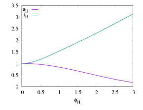
(a) (b)

Figure 1: Two basic quantities of hairy black hole: (a) reduced area of horizon $a_{H}$ and reduced Hawking temperature $t_{H}$ as functions of the scalar field at the horizon $\phi_{H}$. Two are starting with $a_{H}=t_{H}=1$ for the Schwarzschild black hole at $\phi_{H}=0$. (b) horizon radius $r_{H}$ as a function of $\phi_{H}$.

Fig. 1(a) shows the plots of reduced area of horizon $a_{H}$ and reduced Hawking temperature $t_{H}$. We recall that two are $a_{H}=t_{H}=1$ for the Schwarzschild black hole with $\phi_{H}=0$. For increasing $\phi_{H}$, $a_{H}$ decreases monotonically from unity to very close to zero whereas $t_{H}$ increases monotonically from unity. Although some hairy black holes were constructed by different $V(\phi)$ [34], their $a_{H}$ and $t_{H}$ behave qualitatively similar to Fig. 1(a). Fig. 1(b) indicates that the radius of horizon $r_{H}$ of hairy black hole is inversely proportional to $\phi_{H}$, which means that the hairy black holes bifurcates from the Schwarzschild black hole with a very large value of $r_{H}$ and finally, $r_{H}$ could shrink to zero as $\phi_{H}$ increases. Here, both $r_{H}$ and $\phi_{H}$ could take any arbitrary positive real values.

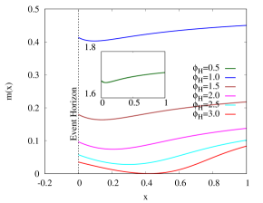
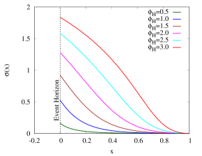
(a) (b) (c)

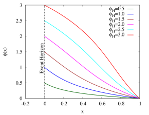
Figure 2: Six solutions with different $\phi_{H}$ of hairy black hole in the compactified coordinate $x$: (a) mass function $m(x)$ contains an inset for $\phi_{H}=0.5$ (b) metric function $\sigma(x)$, and (c) scalar hair $\phi(x)$.

Now, we are in a position to present the numerical solutions and discuss their properties. Fig. 2 exhibits six solutions of hairy black hole with a choice of six different $\phi_{H}$ as functions of the compactified coordinate $x$, where they are regular everywhere outside and on the horizon. The functions $\sigma(x)$ and $\phi(x)$ decrease monotonically from its maximum value at the horizon to zero at the infinity. However, the mass function $m(x)$ possesses a local minimum which moves away from the horizon to the infinity as $\phi_{H}$ increases.

We might understand the presence of scalarized black holes by observing the WEC.

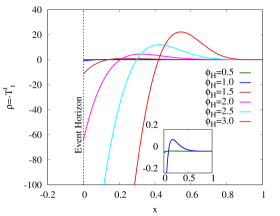
Figure 3: The energy density $\rho$ for the hairy black holes with six $\phi_{H}$ in the compactified coordinate $x\in[0,1]$. The inset shows $\rho$ for $\phi_{H}=0.5,1.0$.

We examine the energy condition of the hairy black hole as shown in Fig. 3. The WEC is described by the energy density $\rho=-T^{t}\,_{t}=N\phi^{\prime 2}/2+V(\phi)$ which is negative near the horizon. This shows violation of the WEC clearly. One may evade no-hair theorem if the scalar matter does not satisfy the WEC [41]. This implies the presence of scalarized black holes. $\rho$ at the horizon decreases very sharply with the increase of $\phi_{H}$. Besides, $\rho$ possesses a local maximum which is located exactly at the local minimum of $m(x)$, and it moves further away from the horizon to the infinity as $\phi_{H}$ increases.

4 Radial perturbations around scalarized black holes

For further implications of scalarized black holes, we need to perform stability test for them. For this purpose, we introduce radial perturbations defined by

$$ds^{2} = -N(r)e^{-2\sigma(r)}\left[1+\epsilon e^{-i\omega t}F_{t}(r)\right]dt^{2}+\frac{1}{N(r)}\left[1+\epsilon e^{-i\omega t}F_{r}(r)\right]dr^{2}+r^{2}d\Omega_{2}^{2},$$ (30)

$$\Phi = \phi(r)+\epsilon\Phi_{1}(r)e^{-i\omega t},$$ (31)

where $F_{t}(r)$, $F_{r}(r)$, and $\Phi_{1}(r)$ are three perturbed fields.

Substituting Eqs.(30) and (31) into (3) and (4), we obtain three linearized equations

$$F_{r} = 8\pi Gr\phi^{\prime}\Phi_{1},$$ (32)

$$F^{\prime}_{t} = -F^{\prime}_{r}+16\pi Gr\phi^{\prime}\Phi^{\prime}_{1},$$ (33)

$$\Phi^{\prime\prime}_{1} = \left(\sigma^{\prime}-\frac{N^{\prime}}{N}-\frac{2}{r}\right)\Phi^{\prime}_{1}+\left(\frac{1}{N}V^{\prime\prime}(\phi)-\omega^{2}\frac{e^{2\sigma}}{N^{2}}\right)\Phi_{1}+V^{\prime}(\phi)\frac{F_{r}}{N}+\phi^{\prime}\frac{F^{\prime}_{r}-F^{\prime}_{t}}{2}.$$ (34)

We eliminate the last two terms in Eq.(34) by making use of the first two equations to obtain an independent scalar equation. Then, we can transform $\Phi^{\prime\prime}_{1}$ to Schrödinger-like equation by introducing $Z(r)=r\Phi_{1}(r)$ and a tortoise coordinate $r_{*}$ defined by $r_{*}=\int dr[\frac{e^{\sigma}}{N}]$ as

$$\frac{d^{2}Z}{dr_{*}^{2}}+\Big{[}\omega^{2}-V_{R}(r)\Big{]}Z=0$$ (35)

with the effective potential

$$V_{\rm R}(r)=Ne^{-2\sigma}\left[\frac{N}{r}\left(\frac{N^{\prime}}{N}-\sigma^{\prime}\right)-8\pi GrN\phi^{\prime 2}\left(\frac{N^{\prime}}{N}+\frac{1}{r}-\sigma^{\prime}\right)+16\pi Gr\phi^{\prime}V^{\prime}(\phi)+V^{\prime\prime}(\phi)\right].$$ (36)

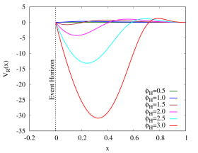
(a) (b)

Figure 4: (a) The effective potential $V_{R}(x)$ with six different $\phi_{H}$ in the compactified coordinate $x\in[0,1]$ for the Schrödinger-like equation. (b) The eigenvalue $\omega^{2}$ for unstable modes as a function of $\phi_{H}$. It is obvious that $\omega^{2}<0$.

We wish to perform the linear stability of the hairy black hole. Before we procced, it is worth mentioning that as Fig. 4(a) is shown, the effective potentials $V_{R}(x)$ with six different $\phi_{H}$ are always negative in some regions of $x$, implying the possible presence of unstable modes. We note that solving Eq.(35) corresponds to handling an eigenvalue problem. Hence, we obtain the radial mode numerically by using COLSYS to solve it with $\omega^{2}$ as an eigenvalue. For black holes, we impose that the perturbation fields vanish at two boundaries, $Z(r_{H})=Z(\infty)=0$. In the numerics, we introduce an auxiliary equation of $\frac{d}{dr}[\omega^{2}]=0$. This allows us to impose an additional condition of $Z(r_{p})=1$ at some point $r_{p}$, which is typically located at the middle of the horizon and infinity. This allows us to obtain a nontrivial and normalizable solution for $Z$, since Eq. (35) is homogeneous. The eigenvalue $\omega^{2}$ is determined automatically when $Z$ satisfies all asymptotic boundary conditions. Accordingly, Fig. 4(b) indicates that the $\omega^{2}<0$ (unstable modes) decreases with the increase of $\phi_{H}$ where the scalar perturbation increases exponentially with time. The perturbation $Z$ is unstable because $\omega^{2}=-\Omega^{2}<0$ where the time-dependent perturbation ($e^{\Omega t}$) grows exponentially with time. This implies that all scalarized black holes belonging to a single branch are unstable.

5 Discussions

We have explored scalarized black holes in the Einstein-minimally coupled scalar theory with a negative potential $V(\phi)=-\alpha^{2}\phi^{6}$. The tachyonic instability is absent from analyzing the linearized scalar equation. In this case, one could not meet a condition for spontaneous scalarization and thus, the linearized stability provided no further information on scalarization.

However, this negative scalar potential with $\alpha=1$ violates the weak energy condition (WEC). It is well-known that if the WEC for a scalar matter is violated, scalarized black holes could be found from the Einstein-minimally coupled scalar theory without introducing a non-minimal scalar coupling to matter. Thus, we have obtained the black hole solutions with scalar hair by solving three nonlinear equations. It includes a single branch of scalarized black holes only because tachyonic intability is absent. Different scalarized black holes are encoded in different $\phi_{H}$ because we have chosen $\alpha=1$. Furthermore, we have studied their thermodynamic properties by introducing reduced horizon area and Hawking temperature.

Then, we have performed the stability analysis for scalarized black holes by adopting radial perturbations. It turned out that six scalarized black holes with six different $\phi_{H}$ belonging to a single branch are unstable. Therefore, it is unlikely that this scalarized black hole can be considered as the astrophysical black holes such as M87 and SgrA*, since the detection on their existence from the astrophysical signatures could be very challenging.

Finally, it would be interesting to obtain the other solutions of scalarized black holes by choosing a more simpler form of the potential, for instance $V(\phi)=-m^{2}_{\phi}\phi^{2},-\Lambda\phi^{4}$ with $m^{2}_{\phi}$ and $\Lambda$ are positive constants, since the previous analysis of Eqs.(8) and (9) in [38] doesn’t rule out the possible existence of scalarized black hole solutions. Therefore, it is worth to investigate such possibilities and report them in the future.

Acknowledgments

XYC acknowledges the support from the starting grant of Jiangsu University of Science and Technology (JUST).

References

- [1] W. Israel, Phys. Rev. 164, 1776-1779 (1967) doi:10.1103/PhysRev.164.1776
- [2] B. Carter, Phys. Rev. Lett. 26, 331-333 (1971) doi:10.1103/PhysRevLett.26.331
- [3] R. Ruffini and J. A. Wheeler, Phys. Today 24, no.1, 30 (1971) doi:10.1063/1.3022513
- [4] C. A. R. Herdeiro and E. Radu, Int. J. Mod. Phys. D 24, no.09, 1542014 (2015) doi:10.1142/S0218271815420146 [arXiv:1504.08209 [gr-qc]].
- [5] N. M. Bocharova, K. A. Bronnikov and V. N. Melnikov, Vestn. Mosk. Univ. Ser. III Fiz. Astron. , no. 6, 706 (1970).
- [6] J. D. Bekenstein, Annals Phys. 82, 535-547 (1974) doi:10.1016/0003-4916(74)90124-9
- [7] G. Antoniou, A. Bakopoulos and P. Kanti, Phys. Rev. Lett. 120, no.13, 131102 (2018) doi:10.1103/PhysRevLett.120.131102 [arXiv:1711.03390 [hep-th]].
- [8] D. D. Doneva and S. S. Yazadjiev, Phys. Rev. Lett. 120, no.13, 131103 (2018) doi:10.1103/PhysRevLett.120.131103 [arXiv:1711.01187 [gr-qc]].
- [9] H. O. Silva, J. Sakstein, L. Gualtieri, T. P. Sotiriou and E. Berti, Phys. Rev. Lett. 120, no.13, 131104 (2018) doi:10.1103/PhysRevLett.120.131104 [arXiv:1711.02080 [gr-qc]].
- [10] J. L. Blázquez-Salcedo, D. D. Doneva, J. Kunz and S. S. Yazadjiev, Phys. Rev. D 98 (2018) no.8, 084011 doi:10.1103/PhysRevD.98.084011 [arXiv:1805.05755 [gr-qc]].
- [11] C. A. R. Herdeiro, E. Radu, N. Sanchis-Gual and J. A. Font, Phys. Rev. Lett. 121, no.10, 101102 (2018) doi:10.1103/PhysRevLett.121.101102 [arXiv:1806.05190 [gr-qc]].
- [12] Y. S. Myung and D. C. Zou, Phys. Rev. D 98, no.2, 024030 (2018) doi:10.1103/PhysRevD.98.024030 [arXiv:1805.05023 [gr-qc]].
- [13] Y. S. Myung and D. C. Zou, Eur. Phys. J. C 79, no.3, 273 (2019) doi:10.1140/epjc/s10052-019-6792-6 [arXiv:1808.02609 [gr-qc]].
- [14] D. C. Zou and Y. S. Myung, Phys. Rev. D 102, no.6, 064011 (2020) doi:10.1103/PhysRevD.102.064011 [arXiv:2005.06677 [gr-qc]].
- [15] H. Witek, L. Gualtieri, P. Pani and T. P. Sotiriou, Phys. Rev. D 99, no.6, 064035 (2019) doi:10.1103/PhysRevD.99.064035 [arXiv:1810.05177 [gr-qc]].
- [16] H. O. Silva, H. Witek, M. Elley and N. Yunes, Phys. Rev. Lett. 127, no.3, 031101 (2021) doi:10.1103/PhysRevLett.127.031101 [arXiv:2012.10436 [gr-qc]].
- [17] H. J. Kuan, D. D. Doneva and S. S. Yazadjiev, Phys. Rev. Lett. 127, no.16, 161103 (2021) doi:10.1103/PhysRevLett.127.161103 [arXiv:2103.11999 [gr-qc]].
- [18] W. E. East and J. L. Ripley, Phys. Rev. Lett. 127, no.10, 101102 (2021) doi:10.1103/PhysRevLett.127.101102 [arXiv:2105.08571 [gr-qc]].
- [19] J. L. Blázquez-Salcedo, D. D. Doneva, S. Kahlen, J. Kunz, P. Nedkova and S. S. Yazadjiev, Phys. Rev. D 102 (2020) no.2, 024086 doi:10.1103/PhysRevD.102.024086 [arXiv:2006.06006 [gr-qc]].
- [20] K. V. Staykov, J. L. Blázquez-Salcedo, D. D. Doneva, J. Kunz, P. Nedkova and S. S. Yazadjiev, Phys. Rev. D 105 (2022) no.4, 044040 doi:10.1103/PhysRevD.105.044040 [arXiv:2112.00703 [gr-qc]].
- [21] J. L. Blázquez-Salcedo, D. D. Doneva, J. Kunz and S. S. Yazadjiev, Phys. Rev. D 105 (2022) no.12, 124005 doi:10.1103/PhysRevD.105.124005 [arXiv:2203.00709 [gr-qc]].
- [22] R. A. Konoplya and A. Zhidenko, Phys. Rev. D 100, no.4, 044015 (2019) doi:10.1103/PhysRevD.100.044015 [arXiv:1907.05551 [gr-qc]].
- [23] J. L. Blázquez-Salcedo, S. Kahlen and J. Kunz, Eur. Phys. J. C 79 (2019) no.12, 1021 doi:10.1140/epjc/s10052-019-7535-4 [arXiv:1911.01943 [gr-qc]].
- [24] D. Astefanesei, J. L. Blázquez-Salcedo, C. Herdeiro, E. Radu and N. Sanchis-Gual, JHEP 07 (2020), 063 doi:10.1007/JHEP07(2020)063 [arXiv:1912.02192 [gr-qc]].
- [25] J. Luis Blázquez-Salcedo, C. A. R. Herdeiro, S. Kahlen, J. Kunz, A. M. Pombo and E. Radu, Eur. Phys. J. C 81 (2021) no.2, 155 doi:10.1140/epjc/s10052-021-08952-w [arXiv:2008.11744 [gr-qc]].
- [26] Q. Gan, P. Wang, H. Wu and H. Yang, Phys. Rev. D 104, no.2, 024003 (2021) doi:10.1103/PhysRevD.104.024003 [arXiv:2104.08703 [gr-qc]].
- [27] Q. Gan, P. Wang, H. Wu and H. Yang, Phys. Rev. D 104, no.4, 044049 (2021) doi:10.1103/PhysRevD.104.044049 [arXiv:2105.11770 [gr-qc]].
- [28] Y. Z. Li and X. M. Kuang, Eur. Phys. J. C 84 (2024) no.3, 271 doi:10.1140/epjc/s10052-024-12627-7 [arXiv:2401.07495 [gr-qc]].
- [29] T. T. Sui, Z. L. Wang and W. D. Guo, [arXiv:2311.10946 [gr-qc]].
- [30] J. Sultana, Phys. Rev. D 101, no.8, 084027 (2020) doi:10.1103/PhysRevD.101.084027
- [31] Y. S. Myung and D. C. Zou, Phys. Rev. D 100, no.6, 064057 (2019) doi:10.1103/PhysRevD.100.064057 [arXiv:1907.09676 [gr-qc]].
- [32] A. Corichi, U. Nucamendi and M. Salgado, Phys. Rev. D 73, 084002 (2006) doi:10.1103/PhysRevD.73.084002 [arXiv:gr-qc/0504126 [gr-qc]].
- [33] S. S. Gubser, Class. Quant. Grav. 22 (2005), 5121-5144 doi:10.1088/0264-9381/22/23/013 [arXiv:hep-th/0505189 [hep-th]].
- [34] X. Y. Chew, D. h. Yeom and J. L. Blázquez-Salcedo, Phys. Rev. D 108, no.4, 044020 (2023) doi:10.1103/PhysRevD.108.044020 [arXiv:2210.01313 [gr-qc]].
- [35] X. Y. Chew and D. h. Yeom, [arXiv:2401.09039 [gr-qc]].
- [36] L. Del Grosso and P. Pani, Phys. Rev. D 108 (2023) no.6, 064042 doi:10.1103/PhysRevD.108.064042 [arXiv:2308.15921 [gr-qc]].
- [37] E. Berti, V. De Luca, L. Del Grosso and P. Pani, [arXiv:2404.06979 [gr-qc]].
- [38] X. Y. Chew and K. G. Lim, Phys. Rev. D 109 (2024) no.6, 064039 doi:10.1103/PhysRevD.109.064039 [arXiv:2307.13972 [gr-qc]].
- [39] X. Y. Chew and K. G. Lim, Universe 10 (2024), 212 doi:10.3390/universe10050212 [arXiv:2405.06407 [gr-qc]].
- [40] V. Dzhunushaliev, V. Folomeev, R. Myrzakulov and D. Singleton, JHEP 07 (2008), 094 doi:10.1088/1126-6708/2008/07/094 [arXiv:0805.3211 [gr-qc]].
- [41] J. D. Bekenstein, Phys. Rev. D 51, no.12, R6608 (1995) doi:10.1103/PhysRevD.51.R6608
- [42] O. Bechmann and O. Lechtenfeld, Class. Quant. Grav. 12 (1995), 1473-1482 doi:10.1088/0264-9381/12/6/013 [arXiv:gr-qc/9502011 [gr-qc]].
- [43] H. Dennhardt and O. Lechtenfeld, Int. J. Mod. Phys. A 13 (1998), 741-764 doi:10.1142/S0217751X98000329 [arXiv:gr-qc/9612062 [gr-qc]].
- [44] K. A. Bronnikov and G. N. Shikin, Grav. Cosmol. 8 (2002), 107-116 [arXiv:gr-qc/0109027 [gr-qc]].
- [45] C. Martinez, R. Troncoso and J. Zanelli, Phys. Rev. D 70 (2004), 084035 doi:10.1103/PhysRevD.70.084035 [arXiv:hep-th/0406111 [hep-th]].
- [46] V. V. Nikonov, J. V. Tchemarina and A. N. Tsirulev, Class. Quant. Grav. 25 (2008), 138001 doi:10.1088/0264-9381/25/13/138001
- [47] A. Anabalon and J. Oliva, Phys. Rev. D 86 (2012), 107501 doi:10.1103/PhysRevD.86.107501 [arXiv:1205.6012 [gr-qc]].
- [48] O. S. Stashko and V. I. Zhdanov, Gen. Rel. Grav. 50 (2018), 105 doi:10.1007/s10714-018-2425-x [arXiv:1702.02800 [gr-qc]].
- [49] C. Gao and J. Qiu, Gen. Rel. Grav. 54 (2022) no.12, 158 doi:10.1007/s10714-022-03043-x [arXiv:2111.11582 [gr-qc]].
- [50] T. Karakasis, G. Koutsoumbas and E. Papantonopoulos, Phys. Rev. D 107 (2023) no.12, 124047 doi:10.1103/PhysRevD.107.124047 [arXiv:2305.00686 [gr-qc]].
- [51] A. N. Atmaja, Eur. Phys. J. C 84 (2024) no.5, 456 doi:10.1140/epjc/s10052-024-12809-3 [arXiv:2310.12476 [gr-qc]].
- [52] X. Li and J. Ren, [arXiv:2312.12894 [gr-qc]].
- [53] X. P. Rao, H. Huang and J. Yang, [arXiv:2403.11770 [gr-qc]].
- [54] M. Bouhmadi-López, C. Y. Chen, X. Y. Chew, Y. C. Ong and D. h. Yeom, JCAP 10 (2021), 059 doi:10.1088/1475-7516/2021/10/059 [arXiv:2108.07302 [gr-qc]].
- [55] G. Dotti and R. J. Gleiser, Class. Quant. Grav. 22, L1 (2005) doi:10.1088/0264-9381/22/1/L01 [arXiv:gr-qc/0409005 [gr-qc]].
- [56] T. Regge and J. A. Wheeler, Phys. Rev. 108, 1063-1069 (1957) doi:10.1103/PhysRev.108.1063
- [57] F. J. Zerilli, Phys. Rev. Lett. 24, 737-738 (1970) doi:10.1103/PhysRevLett.24.737
- [58] C. V. Vishveshwara, Phys. Rev. D 1, 2870-2879 (1970) doi:10.1103/PhysRevD.1.2870
- [59] O. J. Kwon, Y. D. Kim, Y. S. Myung, B. H. Cho and Y. J. Park, Phys. Rev. D 34, 333-342 (1986) doi:10.1103/PhysRevD.34.333
- [60] U. Ascher, J. Christiansen and R. D. Russell, Math. Comput. 33, no.146, 659-679 (1979)