Investigating the accelerated expansion of the Universe through updated constraints on viable models within the Palatini formalism
Abstract
The observed accelerated expansion of the Universe at present epoch can be explained by some of the models without invoking the existence of dark energy or any other such exotic component in cosmic fluid. The models in Palatini formalism is relatively less explored in recent times with respect to their counterpart in metric formalism. We study seven models in Palatini formalism: Hu–Sawicki (two cases), Starobinsky, exponential, Tsujikawa, , and . Following standard statistical procedure and utilizing data sets: type Ia supernovae data, cosmic chronometer observations, baryonic acoustic oscillations data, data from H ii starburst galaxies, local measurements of the Hubble parameter (), and distance priors of cosmic microwave background radiation data, we obtain constraints on the model parameters. When compared with the standard ‘lambda-cold dark matter model’, for many data set combinations, the support for models is significant. We obtain the relevant quantities for characterizing the accelerated expansion of the Universe, and these quantities are consistent with those obtained in a model-independent way by others. The curve of effective/total equation- of-state parameter, obtained from parameter constraints, clearly shows correct phases of the expansion history: the radiation-dominated epochs and the matter-dominated epochs, of the past, and the current accelerated expansion epoch eventually evolving to de-Sitter phase in the distant future. Overall, our results advocate in favour of pursuing models in Palatini formalism as a potential alternative for explaining accelerated expansion of the Universe.
Ramakrishna Mission Vivekananda Educational and Research Institute, Belur Math 711202, Howrah, West Bengal, India
Keywords: dark energy theory, modified gravity, Palatini formalism, cosmological models, baryon acoustic oscillations, supernova type Ia - standard candles
1 Introduction
By the end of last millennium, it was evident that the Universe is currently going through an accelerated phase of expansion. The discovery from the observations of type Ia supernovae (SNIa) [1, 2, 3, 4], has been further validated by subsequent cosmological observations, for instance, observation of baryonic acoustic oscillations (BAOs) [5, 6], analysis of cosmic microwave background (CMB) radiation [7, 8, 9, 10], and examination of the power spectrum of matter distributions in the Universe [11, 12]. Any attempt to explain the accelerated expansion within the framework of Einstein’s gravity, requires inclusion of a hypothetical fluid (generally called ‘dark energy’) with negative pressure, which can counteract the gravitational pull to provide accelerated expansion.
With re-inclusion of, formerly abandoned term by Einstein, in his field equation of gravity, we get the ‘lambda-cold dark matter (CDM) model’ of Cosmology. Although this simplest model provides explanation of above phenomena and also fits to all major observed cosmological data very well (i.e. with respect to goodness of fit analysis), nevertheless, this model faces at least two serious issues, namely, the cosmological constant problem, and the cosmic coincidence problem. With regards to particle physics, it is expected that the cosmological constant should be identified with the vacuum-energy. Then the quantum electrodynamical calculations estimate the density of this vacuum-energy is to be , whereas the measurements from cosmological data yield a value , that is, a discrepancy of 120 orders of magnitude! This embarrassing discrepancy between measured value and theoretical estimate, is called as the cosmological constant problem [13]. In the CDM model, the density of matter contents of the Universe evolves as , where denotes redshift, while the density corresponding to the term remains constant throughout. And yet the cosmological measurements yield their current fractional densities to be of same order, for the former and for the latter. To many researchers this coincidence appear puzzling for various reasons, and is termed as the cosmic coincidence problem [14].
This inadequacy of the CDM model has ended-up motivating researchers to explore many alternative models or theories. We list some broad categories of theories/models which have been in practice in this regards. (i) A first simpler class of alternative models proposed, consists of replacing of the CDM model with variable, parameterized, . For instance the popular Chevalier– Polarski–Linder model [15, 16] has with model parameters . There are many such proposals with its pros and cons (see [17], and references therein). These class of models are dubbed as ‘parametric dark energy models’ in the literature. (ii) Derived from incorporating a scalar field to the energy-momentum tensor of the Einstein equation, the so-called scalar field models, are also being researched for explaining the accelerated expansion. The two subclasses of these models, quintessence models [18] and k-essence models [19], differ in a sense that unlike the former, the latter are derived from Lagrangians with noncanonical kinematic terms. (iii) Shortly after the discovery of accelerated expansion of the Universe, in 1999, it was also proposed to relax the standard assumption of the so-called Copernican Principle (CP, i.e. the assumption that at large enough scales, the Universe is homogeneous and isotropic) and consequently, in this approach, inclusion of large-scale nonlinear inhomogeneities, resulted in explaining away the effects of dark energy [20, 21]. These shorts of theories involve working with the spherically symmetric Lemaître–Tolman–Bondi (LTB) metric rather than the usual Friedmann–Lemaître–Robertson–Walker (FLRW) metric. A limitation or drawback of this approach, apart from violating of the CP, is often quoted as the requirement of placing the observer at a centre of 1-3 Gpc wide void. For a review or more on this field of research, known as ‘inhomogeneous cosmology’, one can see [22, 23, 24, 25, 26]. (iv) There are also modified gravity theories, derived from including higher order corrections to the Einstein–Hilbert (EH) action. The modified gravity theories provide acceleration through geometry itself. One of the simplest of these theories involve replacing the Ricci scalar, , in the EH action, by an arbitrary function , known as ‘ gravity’. Originally proposed in context of cosmic inflation, with the discovery of accelerated expansion of the Universe, gravity models have evolved into an active area of research for the latter context too.
Within the framework of this so-called gravity, one can assume that the Christoffel connections are derived from the metric itself and subsequently vary the Einstein–Hilbert action with respect to metric, only, to obtain the field equations. This approach is called ‘metric formalism’ of the gravity. Alternatively, one can also treat the Christoffel connections and the metric as independent, and vary the Einstein– Hilbert action with respect to each to get the governing field equations. This latter approach is termed as ‘Palatini formalism’ of the gravity. For the CDM model where , both of these approaches provide same sort of field equations, whereas for any other , they provide quite different sets of governing equations. To be specific, while in the metric formalism the resultant modified Friedmann equations include fourth order differential equation, in the Palatini formalism it is only of second order.
In this work, we provide updated constraints on viable gravity models using the latest cosmological data sets, including SNIa from Pantheonplus compilation, cosmic chronometer (CC) observations, BAO data, H ii starburst galaxies (HiiG) data, local measurements of the Hubble parameter (), and the distance priors of CMB radiation (CMBR). We study seven viable models in the Palatini formalism: the Hu– Sawicki model (two cases), the Starobinsky model, the exponential model, the Tsujikawa model, plus two more models which are only viable in the Palatini formalism, namely, and . These models in their original forms give a false impression that they are non-reducible to the CDM model, so we chose to re-parameterize these models in terms of ‘deviation/distortion parameter (b)’. In latter forms, with , we can clearly see, a model tends to the CDM model.
There are fewer past works which have constrained models in the Palatini formalism using observed data. The Hu–Sawicki model in its original form has been constrained in [27], using data of the gas mass fraction in X-ray luminous galaxy clusters, CMB/BAO peaks ratio data, CC data and SNIa data from Union 2.1 catalogue. In [28], the exponential model has been constrained using SNIa data from Union 2 catalogue and CC data. Constraints on the model have been obtained in [29, 30, 31], and [32] using various data sets. The model has been constrained in [30] using a total of 115 SNIa data points, BAO peak data and CMB shift parameter data. We could not find any reference for other three models which we have also included in this work within context of Palatini formalism.
This work is organized as follows. In Section 2 we derive the modified Friedmann equations and other required equations from the Einstein–Hilbert action for gravity. A brief introduction to models investigated in this work is provided in Section 2. We introduce the cosmological data sets and the corresponding equations that establish connection between theory and data, in Section 4, along with discussing the statistical procedures employed to obtain constraints on the model parameters. Resultant constraints on the model parameters, for all the models, are presented in Section 5. Assessment of performance of different models using statistical tools, is provided in Section 6. Section 7 is dedicated to deriving the relevant quantities that characterize expansion history of the Universe based on the model constraints. Finally, we provide the concluding remarks for this work in Section 8.
Unless otherwise specified, we have set (where, denotes speed of light in vacuum), and value of the Hubble parameter is expressed in the unit km s-1Mpc-1.
2 cosmology in the Palatini formalism
The modified version of Einstein–Hilbert action for gravity can be expressed as
| (1) |
where , is the determinant of the metric tensor (), is the action for matter fields and is the action for radiation fields. The symbol stands for generalized Ricci scalar which is derived from the generalized Ricci tensor . We will also be using symbols and for Ricci scalar and Ricci tensor, respectively, derived solely from metric. Unlike metric formalism the connection and the metric are treated as independent fields in Palatini formalism, and so correspondingly, the action has to be varied with respect to (w.r.t.) the metric, and again separately, w.r.t. the connection, to get the governing field equations. Varying the action Eq. 1 w.r.t. metric gives
| (2) |
where and is the energy-momentum tensor of the matter and the radiation from actions and . Variation of action Eq. 1 w.r.t. connection gives
| (3) |
where represents covariant derivatives. The independent connection is given by
| (4) |
where denotes the Christoffel symbols of the metric . The generalized Ricci tensor constructed from the independent connection Eq. 4 is given by
| (5) |
where denotes the covariant D’Alembertian. After contraction of the generalized Ricci tensor Eq. 5 w.r.t. the metric we get the expression for generalized Ricci scalar as
| (6) |
After substitution of Eqs. 5 and 6 into Eq. 2 we get,
| (7) | |||||
where is the Einstein tensor. We assume that the Universe is described by the spatially flat Friedmann–Lemaître–Robertson–Walker (FLRW) metric, given by
| (8) |
We assume the general consideration that the Universe is made up of perfect-fluid with energy density and pressure , and so correspondingly, the enery-momentum tensor simplifies to . For FLRW metric, the - component of tensorial equation (Eq. 7) gives
| (9) |
and ‘’ - component (where ) gives
| (10) |
The overhead dots in above two equations represent derivative w.r.t. ‘’. Combining Eqs. 6, 9 and 10 we get the generalized as Friedmann equation
| (11) |
Assuming the matter content to be pressureless () dust with density and radiation with density and pressure , in the absence of any interaction between matter and radiation after the epoch of decoupling, the conservation equation holds and can be written as
| (12) |
and their solutions can be obtained as and . Defining and , we get and , where the redshift is related to the scale factor via .
Trace of Eq. 2 provides us
| (13) |
since the trace of radiative fluid vanishes. Combining the conservation Eq. 12 with time derivative of Eq. 13, we get
| (14) |
We define dimensionless quantities , and so correspondingly, we get . Combining Eqs. 11 and 14, we get
| (15) |
where,
| (16) |
The derivative of Eq. 13 w.r.t. is
| (17) |
To get or , we need , which can be obtained by solving the ordinary differential equation (ODE) 17. The initial condition for ODE Eq. 17 (i.e., (say)) can be obtained from Eq. 15 with the realization that
| (18) |
where we have used . After solving the nonlinear equation 18 for we can use that in the nonlinear Eq. 13 to obtain . Having obtained and , the ODE Eq. 17 can be solved from to desired to get , and numerically inverting the latter solution provides us .
When using observed data for model constraining we need many cosmological distances, all of which could be defined from the ‘comoving distance’, defined as
| (19) | |||||
where and . Thus, we can get with the help of the solution of ODE Eq. 17.
If we compare the modified Friedmann Eqs. 9 and 10 to the usual Friedmann equations with a dark energy component characterized by energy density and pressure , that is, with the equations and , we can deduce the ‘effective (geometric) dark energy’ with following density and pressure for any model in Palatini formalism:
| (20) |
and,
| (21) |
Correspondingly, we can define equation-of-state parameter for effective dark energy as
| (22) |
where,
| (23) |
is the total equation-of-state parameter, that is, for all the components of cosmic fluid. In the above relation the fractional matter and radiation density functions are defined as: and , which utilizes the fact that and .
3 models
A brief introduction to the seven models investigated in this work is presented here. Apart from presenting the models in their original proposed forms, we also transformed them to forms which make apparent their reducibility to the CDM model. For this we re-parameterized the models in terms of ‘deviation/distortion parameter ()’, where with , all model tends to the CDM model. Eventually, we obtain all the models expressed in terms of , and other parameters. However, from Eq. 13 we can see that , , and are not all independent. Therefore, for reporting the results from data fitting, we choose a seemingly more meaningful parameter combination, that is, , , and other parameters.
3.1 The Hu–Sawicki model
In its original form the Hu–Sawicki model [33], is expressed as
| (24) |
where , , (assumed to be a positive integer) are dimensionless parameters with . In this form it is hard to see how this model could be relatable to the CDM model, and with this need, later a re-parameterization was introduced by [34] as
| (25) |
where and . Although this model have been studied with various cosmological data, very actively in the metric formalism (see [35], and references therein), there is lack of studies of this model in the Palatini formalism [27]. In this work, apart from common practice of taking , we will also constrain the case of . Later we will see that in the re-parameterized versions, the case of here is equivalent to the Starobinsky model.
3.2 The Starobinsky model
In Starobinsky model [36]
| (26) |
where is a positive constant, and ( denotes the Ricci scalar at present epoch) are free parameters. This model can also be represented in a more general form as [34]
| (27) |
where and . In this work, we specifically consider the case where , with the justification for not exploring values of higher than 1 can be found in [35]. From Eqs. 25 and 27, it is clear that the Hu–Sawicki model with and the Starobinsky model with are equivalent. The algebraic form of (Eq. 27) suggests that, irrespective of the data set, from MCMC fitting procedures, one will certainly obtain the parameter distributed symmetrically around . Without loss of generality, we adopt , as we are mainly interested in studying deviation/distinguishabililty from the CDM model. We could not find any earlier work where this model has been constrained in context of the Palatini formalism, whereas there are many such works in the metric formalism (see [35], and references therein).
3.3 The exponential model
The exponential model from [37], widely constrained in context of metric formalism [38, 39, 40, 41] is given by
| (28) |
where and are the parameters of this model. Though with and the identification , it’s reduction to the CDM model is apparent, but still we re-parameterize it with the deviation parameter, , as
| (29) |
with and . In latter form, for finite values of the parameters, the exponential model tends to the CDM model. From this, it is evident that when , , . In the past, exponential model in Palatini formalism has been constrained by [28] for the purpose of dark energy studies.
3.4 The Tsujikawa model
The Tsujikawa model [42] is given by
| (30) |
Here and are the model parameters. By defining and , this model too can be expressed in more general form as
| (31) |
Evidently, as (meaning , but remains finite), the Tsujikawa model simplifies to . We should also note that while doing numerical computations for this model, it is better to express rather than and so on. The former avoids numerical instability while the latter do not, especially for very large and very small values of (for ). Although this model have been constrained enthusiastically in the metric formalism (see [35], and references therein), we could not find any literature which has constrained it in the Palatini formalism.
3.5 Two more models
We also investigate constraints on two alternative models described by (i) and (ii) . Here , and represent the parameters of these models. Although these two models are found to be non-viable in the metric formalism, however, these models are of particular relevance in the Palatini formalism, as they yield a correct sequence of radiation-dominated, matter-dominated, and de-Sitter era in expansion history of the Universe [29, 30, 31, 32]. These two models also can be re-parametrized in terms of and , trivially, as follows:
| (32) |
with identifications and ; and
| (33) |
by recognizing as and as .
4 Observed cosmological data and Statistical analysis
Here we briefly introduce the cosmological data sets utilized in this work to constraint models. For any model, we mainly obtain numerically, using equations 15, 16, 17, and 18. So providing theoretical relations between and various observed quantities becomes imperative, which we also do in this section. Towards the end of this section, we also discuss the statistical methods employed to extract model parameters from data sets.
4.1 Type Ia supernova data
The type Ia Supernovae (SNIa) have been established as a standard candle class of astrophysical objects [43]. In fact, it was the observations of SNIa that led to the discovery of accelerated expansion of the Universe in late 1990s [1, 2, 3, 4]. In this work, we employ apparent magnitude data for SNIa from the recently released PantheonPlus compilation [44]. This latest compilation comprise of 1701 distinct light curves of 1550 uniquely spectroscopically confirmed SNIa from 18 surveys. It offers a broader range of low- redshift data compared to the earlier Pantheon compilation [45], with redshift spanning (where denotes Hubble diagram redshift). We utilize the apparent magnitude at maximum brightness (), along with heliocentric redshift (), cosmic microwave background (CMB) corrected redshift (), and the combined covariance matrix (statistical + systematic) from this compilation [44].
The expression for luminosity distance
| (34) |
which can be obtained with the help of comoving distance () defined in Eq. 19. Theoretically, apparent magnitude () is defined in terms of luminosity distance and expressed as
| (35) |
where is referred to as the absolute magnitude, and is termed as the ‘dimensionless Hubble-free luminosity distance’. In light of inherent degeneracy between the absolute magnitude () and the current epoch Hubble parameter () in the calculation of apparent magnitude (as revealed in Eq. 35), we employ marginalization over parameters and . The subsequent marginalized which requires to be minimized for model fitting, is defined as [46]
| (36) |
where , , and . Here represents the combined covariance matrix, while constitutes an array of ones matching the length of data set. Of course, here, the theoretical estimations of apparent magnitude () are subject to the model under consideration.
4.2 Cosmic chronometers data and local measurement of
By observing the age difference () of passively evolving galaxies (where star formation and interactions with other galaxies have ceased) at redshift difference (), the cosmic chronometers measurements employ the following so-called ‘differential age method’ [47, 48, 49] to obtain Hubble parameter at different redshifts:
| (37) |
So far there have been made a total of 32 such measurements by various researchers [49, 50, 51, 52, 53, 54, 55, 56] in the redshift range of 0.07-1.965. In this study we use these 32 data points comprising of from Table B2 of [35].
For parameter estimations of any model, one can minimize the following residual
| (38) |
where denotes the observed values of the Hubble parameter function at redshift , and denotes the associated uncertainties in these measurements. The theoretical Hubble function at redshift , which is model-dependent and obtained from Eq. 17, is denoted by in the above Eq. 38.
There remains a debatable issue regarding current value of the Hubble parameter, . The Planck constraints suggest [57] (which is inferred from the CMB data assuming standard cosmological model) while the locally measured value from the SH0ES collaboration is [58] (which is obtained from SNIa and Cepheid data in a cosmological model independent way). The two measurements show a tension of indicating a notable discrepancy between them. Considering this apparent Hubble tension, we have incorporated both scenarios, with and without the SH0ES prior for in our investigation. We use following Gaussian prior on for minimization corresponding to the SH0ES data
| (39) |
4.3 ii starburst galaxies data
H ii starburst galaxies (HiiGs) are compact and massive regions where stars form actively and are also surrounded by ionized hydrogen gas. Their optical spectra reveal narrow Balmer lines, such as H and H, amidst a faint continuum. The observed empirical correlation between the luminosity () of the H line and the velocity dispersion ()–a measure of spectral line width–underscores the significance of HiiG data for cosmological investigations. This correlation is understandable, since an increase in the mass of the starburst component leads to heightened emission of ionization-induced photons (thereby enhancing luminosity ) and also augmented turbulence in velocity (resulting in higher velocity dispersion , see [59], and references therein).
This study utilizes a total of 181 data points taken from [59, 60, 61, 62], and [63] of the Balmer H line emission. The redshift coverage of these data points is . One advantage of using HiiG data set could be that it explores higher redshifts, along with relatively denser coverage at higher redshift, when compared with those of SNIa data [35].
The aforementioned empirical correlation between luminosity and velocity dispersion can be expressed as follows:
| (40) |
To obtain luminosity from observed velocity dispersion , we take and from [59, 63]. Having obtained the luminosity, we can derive the luminosity distance using observed value of flux () associated with H line, as . Consequently, the distance modulus of HiiG data set can be obtained as
| (41) |
With theoretical definition of distance modulus , given by Eq. 35, and above derived from observations, we can constraint any cosmological model by minimizing following
| (42) |
The combined variance in the above equation, is comprised as
| (43) |
where,
| (44) |
and,
| (45) |
and [64, 63, 59]. With simple error propagation theory we can derive from Eq. 41, and , stemming from redshift uncertainties (), from the standard relation of in terms of and in terms of .
4.4 CMB data and BAO data
Shortly after Big Bang, the Universe was made-up of hot, dense plasma, consisting mainly of protons, electrons, and photons, and was almost uniformly distributed but with small fluctuations. With Thomson scattering, baryons and photons were tightly coupled. The subsequent expansion caused decrease in temperature and density, and also amplification of fluctuations due to gravity. With pull due to gravitation and push due to radiation pressure, tightly coupled baryon-photon mixture condensed in regions with higher densities and thus creating compressions and rarefactions in the form of acoustic waves referred to as BAOs. Approximately 380,000 years after the Big Bang, the Universe had cooled sufficiently for protons and electrons to combine and form neutral hydrogen atoms. Consequently photons decoupled from baryons. After this transition, known as recombination, photons travelled freely through space without scattering off charged particles. The CMB radiation we observe today are those early decoupled photons, providing a snapshot of the Universe’s state at the epoch of recombination/decoupling (). The CMB or CMBR observed today, is still a blackbody radiation, distributed almost uniformly throughout the Universe at a temperature of 2.73 K, with anisotropies of order of .
After release of baryons from the Compton drag of photons at epoch of drag (, slightly later to ), the acoustic waves remained frozen in the baryons. A characteristic length-scale attributed to BAOs is the sound horizon at the epoch of drag (), defined as the maximum distance travelled by the acoustic wave before decoupling. BAO, hence, holds a status of standard ruler for length-scale in Cosmology ([65, 66]). The primordial density fluctuations in baryons provided the seeds for the formation of cosmic structures, including galaxies, clusters, and superclusters.
We have used a total of 30 data points of various BAO observables from compilation in Table B1 of [35], collected therein from many surveys [67, 68, 69, 70, 71, 72, 73, 74, 75, 76, 77, 78, 79, 80, 81, 82, 83, 84, 85, 86]. To compute the epoch of drag () and the sound horizon at the epoch of drag (), we employ improved fits from [87]. The BAO observables encompass the Hubble distance, defined by and other observables, namely, the transverse comoving distance (), the angular diameter distance (), and the volume-averaged distance (), are defined as follows:
| (46) |
| (47) |
and,
| (48) |
Using Eq. 15, the solution of the ODE given in Eq. 17, and Eq. 19, all of the above observables can be converted from functions of redshift to functions of . This enables their use in constraining the parameters of any model within the Palatini formalism.
To fit any model to the BAO data, the following residuals have been employed for uncorrelated data points:
| (49) |
where and represent the observed values and their respective measurement uncertainties at redshift , and signifies the theoretical prediction derived from the model under consideration. These observed quantities are provided in columns 2 to 4 of aforementioned Table of [35].
For correlated data points, the relevant residual to be minimized, is given by
| (50) |
where ’s represent covariant matrices for the three distinct data sets, while indicates an array of the differences between theoretical and observed values for each of these three sets. The covariance matrices can be found from the respective source papers mentioned in the last column of the Table B2 of [35] and/or from the Eqs. B1, B2 and B3 of [35]. For whole of the BAO data, we utilize following combined
| (51) |
From CMB observables, we use the so-called ‘distance-priors’ of CMB, namely,
| (52) |
where (not to be confused with Ricci scalar) is known as the ‘shift parameter’, and is called ‘acoustic scale’. The baryonic fraction of total matter density (), at present epoch, is denoted by , , and is the transverse comoving distance (defined in Eq. 47) at redshift of the epoch of photon decoupling . The comoving sound horizon at the epoch of decoupling, , defined as
| (53) |
For computational ease, we calculate from popularly used fitting formula given in [65], which is
| (54) |
where
| (55) |
The most recent estimations of distance priors derived in [88] from Planck Mission 2018 data [57] are
| (56) |
with their covariance matrix given by
| (57) |
and where ’s denote the standard errors given in the Eq. 56. Finally, for constraining any model with above CMB data, following function needs be minimized
| (58) |
4.5 Statistical analysis
We estimate model parameters from Markov Chain Monte Carlo (MCMC) samples by maximizing following likelihood function
| (59) |
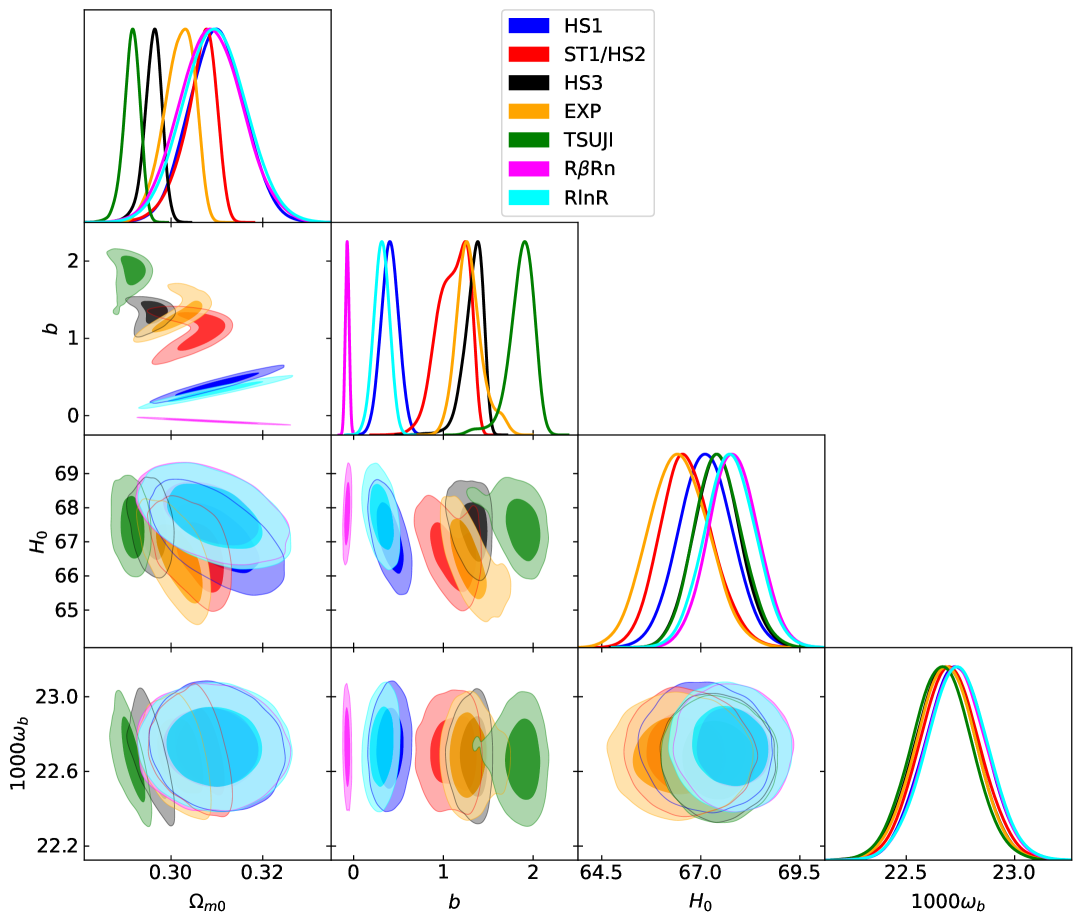
The subscript in Eq. 59 stands for data set combinations from the set: ‘SN’, ‘CC’, ‘SH0ES’, ‘HiiG’, ‘BAO’, ‘CMB’ and corresponding ’s are already defined in Eqs. 36, 38, 39, 42, 51, and 58, respectively. We use uniform priors: , , and . Choosing appropriate priors on deviation parameter, , require some deliberation. So following the logic suggested in [35], and after some initial pilot trails, we choose , where is 1.5, 2, 2, and 2.5 for the models HS1, HS2/ST1, HS3, EXP, and TSUJI, respectively. Here the acronym ‘HS1’ denotes the Hu–Sawicki model with , and similarly the other acronyms for models are defined. For the models (RRn), and (RlnR), we choose and , respectively.
For numerical and statistical computations, we have used some of the publicly available python modules to develop our own python scripts. For solving stiff ODEs we used ‘numbalsoda’ of [89], for generating MCMC samples we utilized emcee [90], and the posterior probability distributions of the parameters are plotted with GetDist [91].
Maximizing above mentioned likelihoods, we generated an initial MCMC sample of size 875,000 (with 25 walkers, each taking 35,000 steps) for each parameters in each case, where by ‘case’ we mean any particular model for a given data set combination. These initial large samples must be tested for convergence and independence. For convergence, we generously discarded first 5000 steps of each walker (i.e. discarding a sample of size 125,000) to obtained the so-called ‘burned chains’. Further to ensure the independence of samples, we thin the burned chains by a factor of 0.75 times the integrated auto- correlation time. Finally, after burning and thinning we obtained, convergent and independent samples of sizes to 20,000. From these latter samples only, we made our statistical inferences about model parameters.
5 Observational constraints
Here we give a detailed account of obtained parameters of all seven models investigated in this work. For assessments of any models, one also needs, as a reference, constraints on the CDM model with same data set. The results of CDM model is not presented here as the same can be found in [35].
Acronyms and colour conventions:
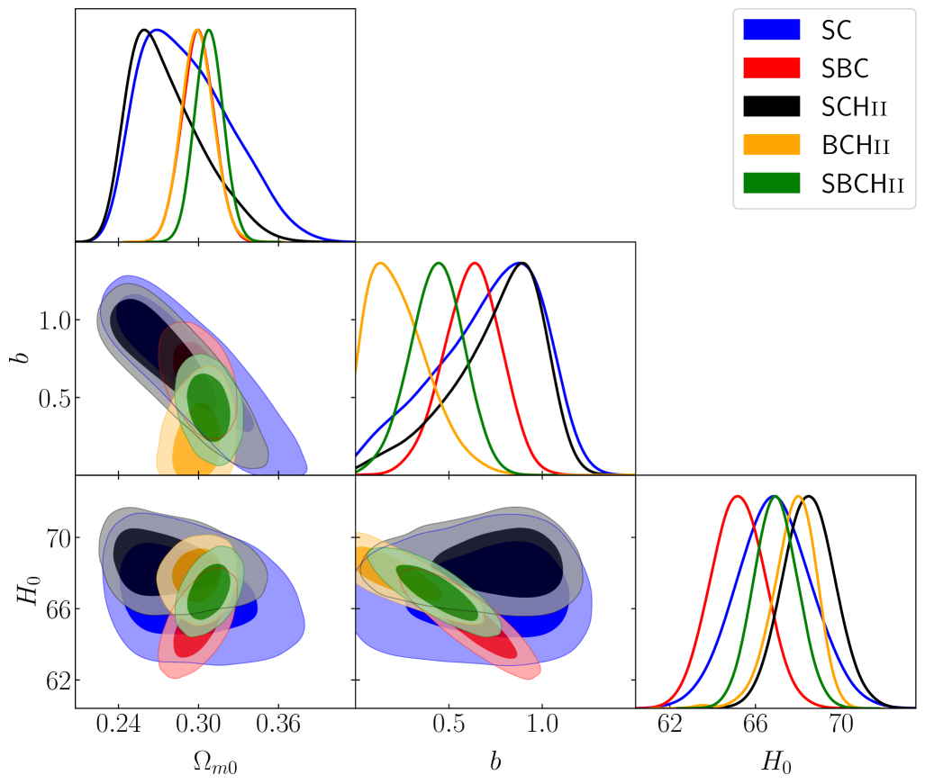
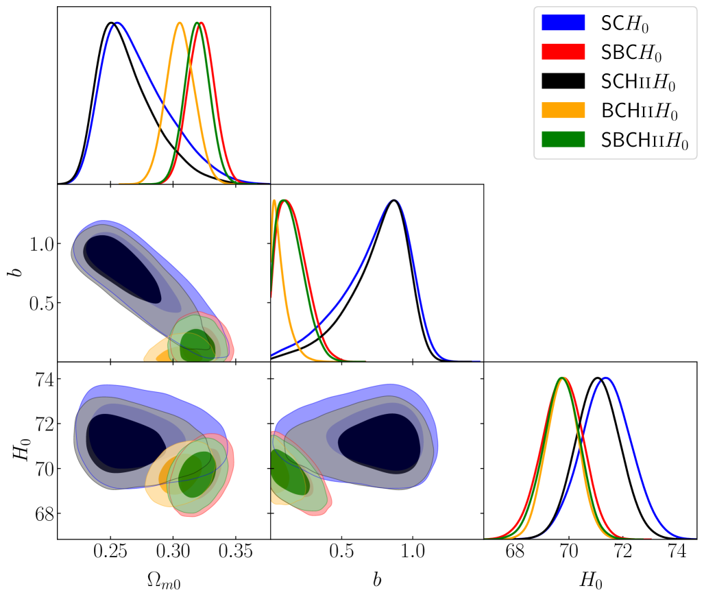
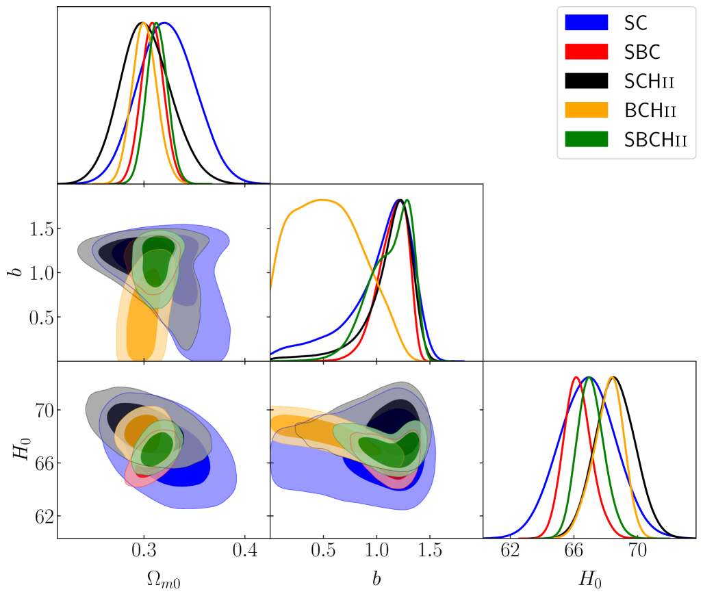
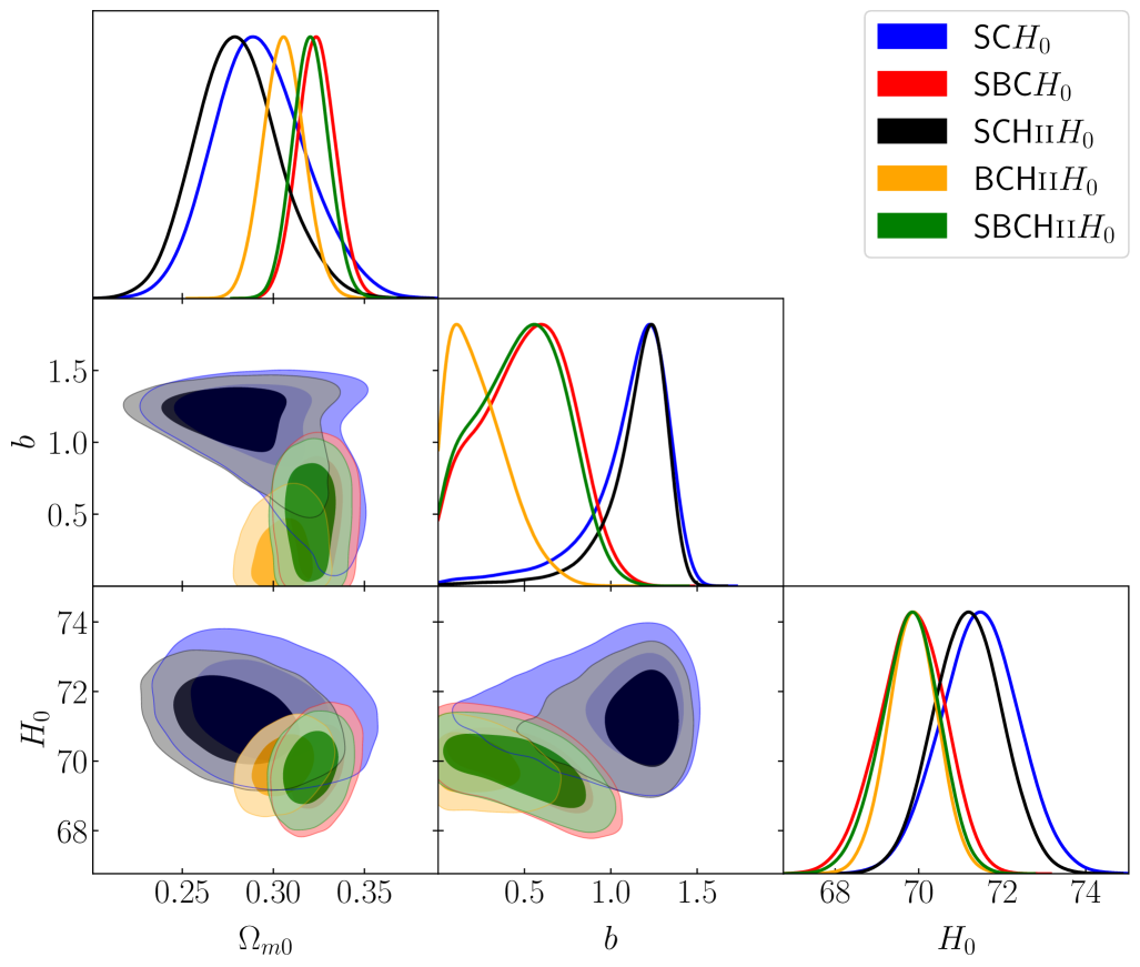
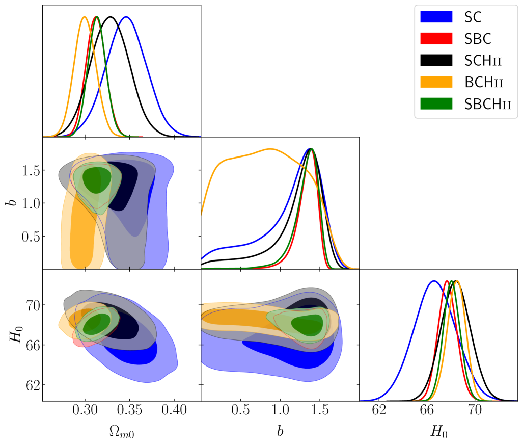
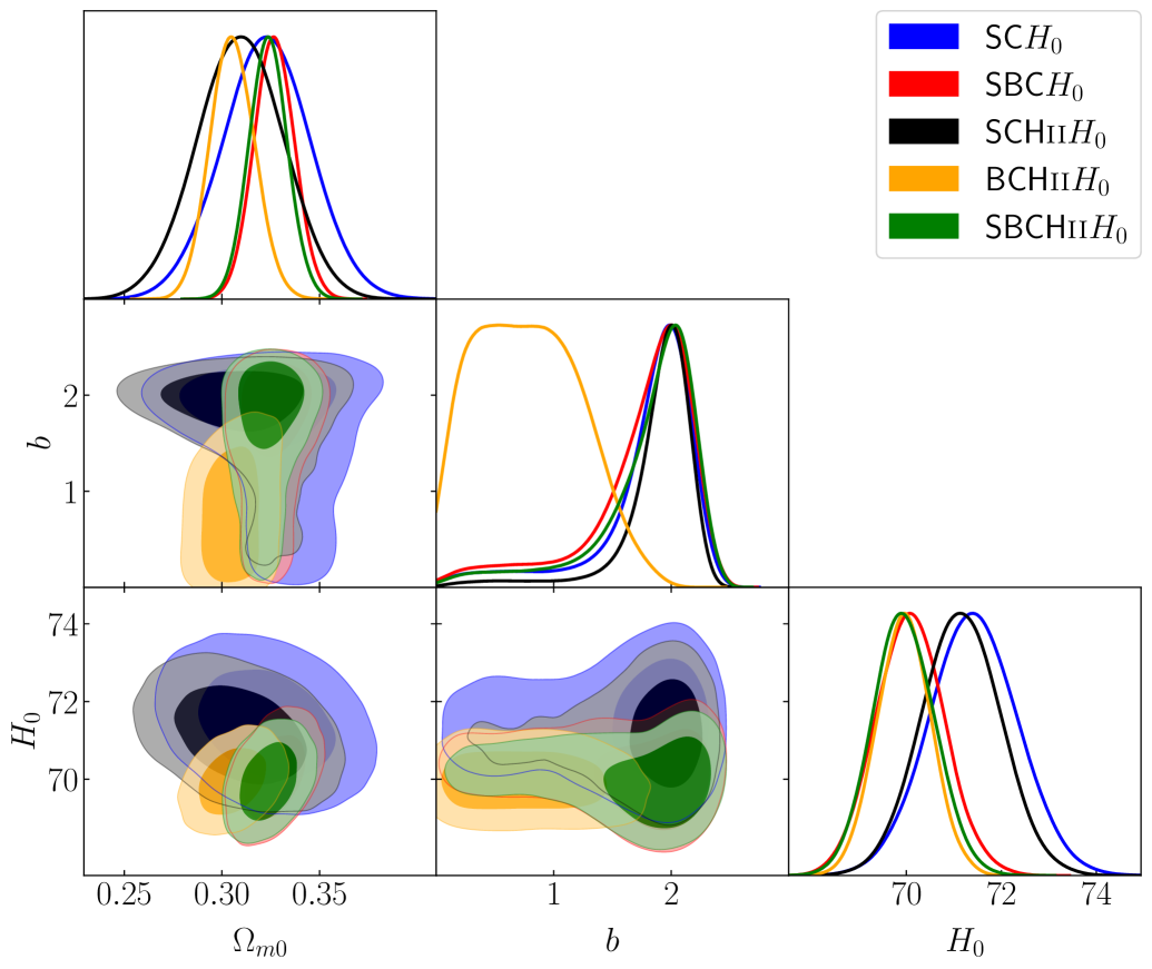
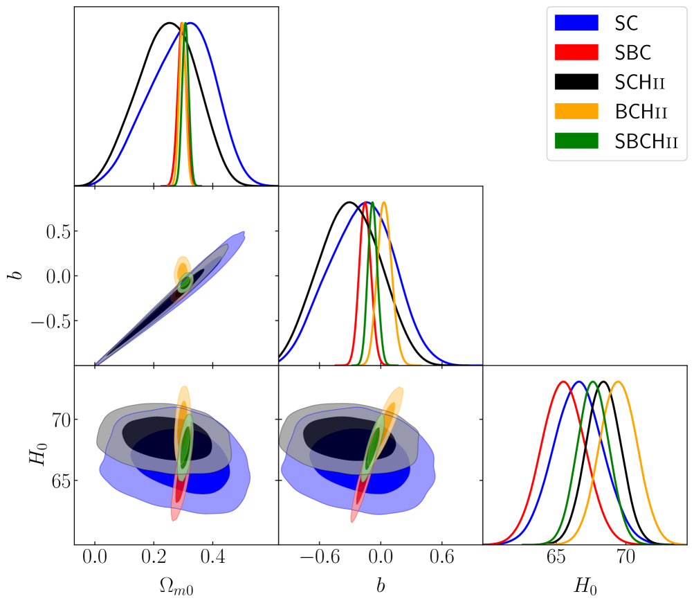
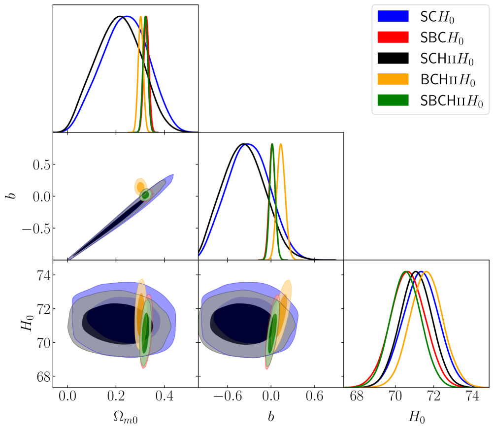
The six data set combinations explored in this work are: (i) SNIa+CC (SC), (ii) SNIa+BAO+CC (SBC), (iii) SNIa+CC+HiiG (SCHii), (iv) BAO+CC+HiiG (BCHii), (v) SNIa+ BAO+CC+HiiG (SBCHii), and (vi) SNIa+BAO+CC+HiiG+CMB (SBCHii+CMB). To study Hubble tension, we also use SH0ES prior for to aforementioned six data sets (so effectively we have explored a total of 12 data set combinations). In addition to above mentioned acronyms for different data set combinations, for denoting data sets with SH0ES prior for included, we append these acronyms with , for example, SC for SNIa+CC+ and SC() to mean SNIa+CC or SNIa+CC+ depending on the context. Unless otherwise specified, in the figures, the following colour and data set correspondences are there: (i) SC() – blue, (ii) SBC() – red, (iii) SCHii() – black, (iv) BCHii() – orange, (v) SBCHii() – green, and (vi) SBCHii()+CMB – brown.
While with six data sets one can explore a total of 63 data set combinations, but our goal is to obtain tighter constraints on model parameters and we also need to be mindful of goodness-of-fit. Thus we decided to explore only six data set combinations and the inclusion of data combination BCH() is to emphasize the fact that not all combinations of data give meaningfully acceptable results.
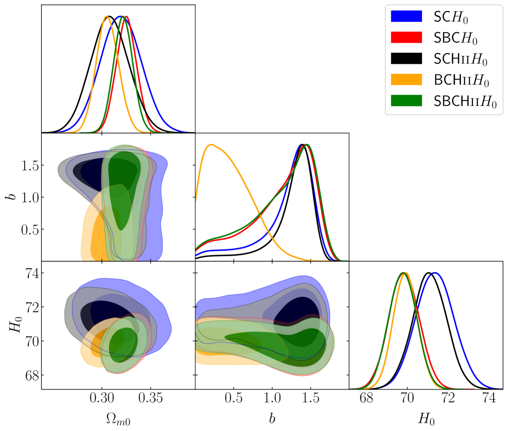
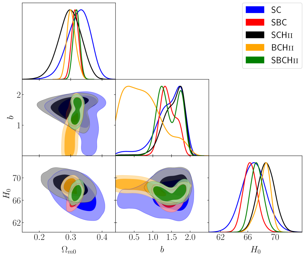
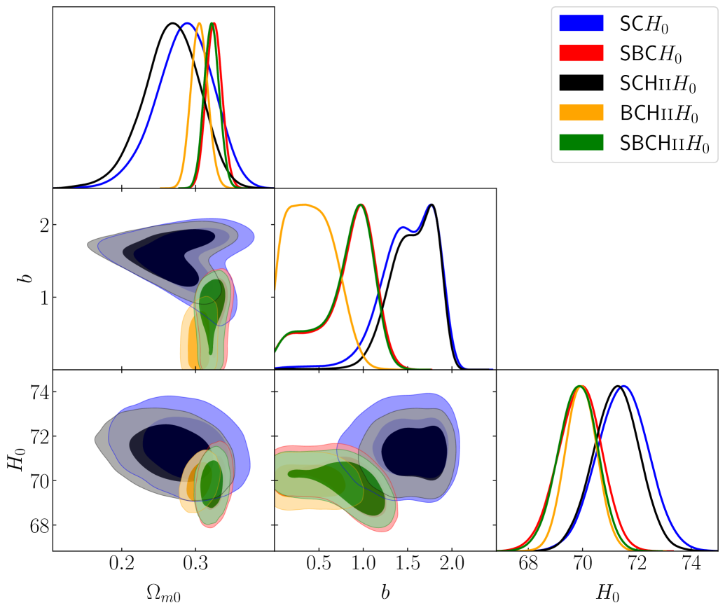
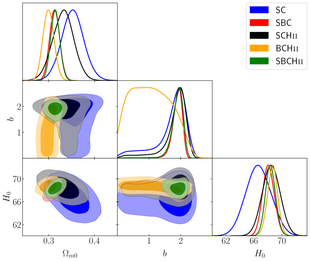
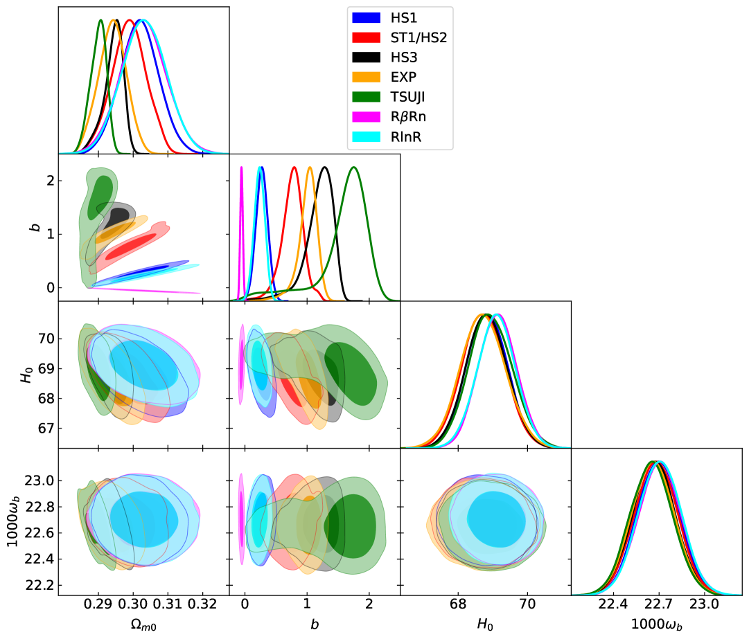
Tables LABEL:resultstable_Pal and LABEL:resultsH0table_Pal present the median values of model parameters along with their corresponding 1 confidence intervals. The posterior probability distribution of model parameters are displayed in Figs. 4-11, where 2D contour plots can be observed to see possible correlations among parameters, and 1D marginal plots can be observed to see symmetry or skewness in distribution of each parameter. Including CMB distance priors in any data combination amounts to constraining a total of four parameters: . Consequently, for the data sets SBCHii+CMB and SBCHii +CMB, for all the models, the posterior probability distributions are shown in Fig. 11. When reading the sections regarding constraints on individual models, the readers are requested to refer Fig. 11 also.
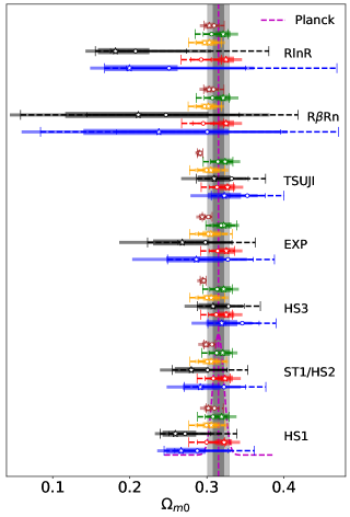
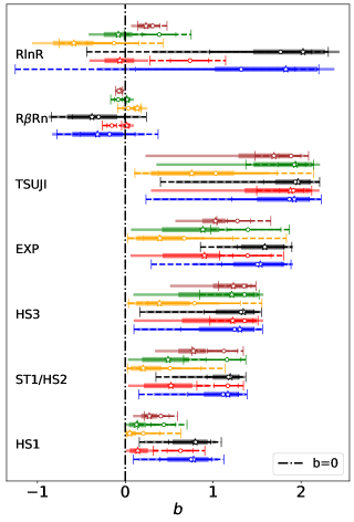
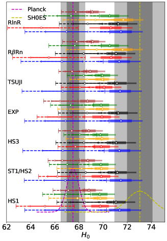
First, considering Figs. 1, and 3, we present a gist of the model predicted parameters and , as how they compare to the standard cosmological measurements like , and – across the models and across the data sets, then we elaborate more on individual models. For most of the cases, the model predicted median values of are within the 1-2 range of the Planck value ( [57]), while for a few cases is within the 1-2 range of the former. When compared with the Planck value of ( [57]), for almost all the models and for most of the data sets without SH0ES prior, the model predicted median values of fall within 1-2 range of the former, while for a few cases its other way round. In contrast, when applying the SH0ES prior on , there are slight departures towards higher values of (as expected), but these values do not closely align with [58]. It’s worth noting that in cases with the SH0ES prior, the bounds on the model values are generally tighter. Additionally, overall there is less tension among model-fitted values of compared to the tension between and . Some trends about the model predicted values of is also worth noting, in light of Fig. 2. When incorporating the SH0ES prior on , there is a consistent tendency for the values to shift towards lower values. This trend is observed in the cases of data sets: SBC, BCH, SBCH, and SBCH+CMB. Conversely, opposite trends are observed for the SC and SCH data sets compared to the corresponding cases without the SH0ES prior on .
5.1 Constraints on Hu–Sawicki and Starobinsky models
Although these models are widely explored in the metric formalism (see [35] and references therein), there is only a few earlier work which has constrained these models in the Palatini formalism [27]. For the reasons discussed in [35], we choose to constraint only cases with and .
The posterior probability distribution plots for HS1, ST1/HS2 and HS3 models are shown in Figs. 4, 5, and 6, respectively, while the quantitative results like median values of the parameters and confidence bound on them are presented in Tables LABEL:resultstable_Pal and LABEL:resultsH0table_Pal. Also see Fig. 11 for results from data sets where CMB is included. Except for model HS3 with data sets SBCHii+CMB and SBCHii+CMB, the matter density parameter, , for these three models (i.e. HS1, ST1/HS2, and HS3), from all the data sets, are compatible with the Planck value of . When SH0ES prior for is not taken, the model predicted median values of are compatible with the Planck value of (covering both values smaller than and bigger than 67.5). From data sets with SH0ES prior, we get relatively tighter constraints on , these model predicted median values of are compatible both and . For latter cases (i.e. with SH0ES prior), model predicted values of are always on lower side of .
Except for the data sets SC and SC, we can observe a general trend of decrease in model predicted median values of when SH0ES prior is included, compared to the corresponding data set without SH0ES prior for . We also observe that for many data sets is only marginally allowed (i.e. is outside the limits), which means we are getting instances of distinguishable HS1, ST1/HS2 and HS3 models from the standard CDM model. Latter in the model comparison chapter we will see that these distinguishable case of HS1, ST1/HS2 and HS3 models, are also (very) strongly supported by AIC, BIC, and/or DIC statistics, so this is an important result of this work. As to be expected, the median values of increases with increase in from 1 to 3 (i.e. from model HS1, to ST1/HS2, to HS3).
For data sets with CMB distance priors, the model predicted median values of decrease – with the inclusion of SH0ES prior, when compared with cases without SH0ES prior. Also there is tend of decreasing with increase in from 1 to 3, alternatively, we can say that models more dissimilar to the CDM model are predicting higher values for .
5.2 Constraints on exponential model
The exponential model is also very extensively constrained in metric formalism (see [35] and references therein), whereas for Palatini formalism we could find a few studies only [28]. We present the quantitative predictions for model parameters in Tables LABEL:resultstable_Pal and LABEL:resultsH0table_Pal. The 2D contour plots of the posterior probability distribution of model parameters () are displayed in the Fig. 7, for the data sets without CMB distance priors, whereas results on parameters (), for data sets with CMB, are displayed Fig. 11.
It is evident from Figs. 2, 7, and 11 that aside from the BCH dataset, the deviation parameter is notably non-zero. The possibility of is only marginally or scarcely allowed. The significance of this outcome will become more apparent in the subsequent chapter dedicated to model comparisons. Nonetheless, the values of the parameters and (see Figs. 1 and 3) are reasonably close to the standard values derived from Planck constraints [57]. When the SH0ES prior on is taken into account, the model’s predictions for hover around approximately 68.5-71.5 km s-1Mpc-1 and always lesser than .
5.3 Constraints on Tsujikawa model
In Tables LABEL:resultstable_Pal and LABEL:resultsH0table_Pal we present the constraints on parameters of the Tsujikawa model outlined in Eq. 31. Additionally, Figs. 8, and 11, respectively for without and with CMB data, depict posterior probability distributions of these parameters. Similar to the findings from the exponential model, we observe here that the deviation parameter, , is non-zero, with zero being allowed only to a very limited extent, for all the datasets except BCH. As for any other models, here also, we disregard the results from BCH due to corresponding high reduced value. Thus, in this case as well, we obtain an model that is distinctly different from the CDM model. The determined values of and also fall within reasonable ranges of and (or ). When considering the SH0ES prior on , the model’s median values for range from approximately 69 to 71.5 km s-1Mpc-1. These values exhibit a tension with or .
5.4 Constraints on model

Though not recently but this model has been widely explored in the past [29, 30, 31, 32], as it successfully produces the latter three phases of the history of the Universe, in Palatini formalism. The model predicted median values of parameters and corresponding confidence bounds, after fitting Eq. 32 to all the data sets, are presented in Tables LABEL:resultstable_Pal and LABEL:resultsH0table_Pal, for data sets without and with SH0ES prior for , respectively. The posterior probability distribution of parameters are shown in the Figs. 9, and 11, respectively for the data sets without and with CMB data. From aforementioned tables and figures (and/or Fig. 1), we can observe that without BAO data, the constraints on is poor, whereas for data sets with BAO included, we are getting reasonably tighter constraints on . Anyway the is always within limits of the model predicted median values. For all the data sets (except SCB, SCBHii()+CMB), is well within limits, that is, we are not getting any instances of this model being significantly different from the CDM model. For three data sets, namely, SCB, SCBHii+CMB, and SCBHii+CMB, is outside confidence interval of model predicted . On account of AIC, BIC and/or DIC, for these three data sets, the results regarding , becomes important only for former two data sets. This model estimates values compatible with , when SH0ES prior is not considered whereas with SH0ES prior, median values of are 69.13-71.33, and are compatible with and/or .
5.5 Constraints on model

This model has been studied earlier in [30] and was shown to be able to produce latter three phase of the Universe and so we have investigated this model with latest data sets. The quantitative results from fitting Eq. 33 to all 12 data sets mentioned earlier, are presented in Tables LABEL:resultstable_Pal and LABEL:resultsH0table_Pal, for data sets without and with SH0ES prior for , respectively. For the data sets excluding and including CMB data, the posterior probability distribution of parameters are shown in the Figs. 10, and 11, respectively. Like the last model, here also the constraints on are poor for the data sets without BAO data, though compatible with , which can be seen from Fig. 1 and above mentioned tables and figures. The only data sets which provides as outside of limits of model predicted median value of (i.e. a case of being significantly distinguishable from the CDM model), are SCBHii+CMB and SCBHii+CMB. Without SH0ES prior, the model predicted median values of are compatible with , whereas with SH0ES priors they are compatible with and/or .
6 Model Comparison
The standard statistical tools, more frequently used in cosmology for the purpose of assessing quality of model fitting and model comparisons, are the reduced chi-square statistics (), the Akaike Information Criterion (AIC, [92]), the Bayesian Information Criterion (BIC, [93]), and the Deviance Information Criterion (DIC, [94]) (also see [95, 96, 97]). We have presented these quantities and other such related quantities in the last eight columns of Tables LABEL:resultstable_Pal and LABEL:resultsH0table_Pal. While the reduced chi-square statistics is simply , the AIC, the BIC and the DIC are defined by the following equations
| (60) |
| (61) |
and,
| (62) |
In the above definitions, the number of degrees of freedom, , is obtained by subtracting the number of model parameters () from the total number of data points (). The minimum value of , , is related to the maximum likelihood () as . In the definition of DIC, is called ‘an effective number of parameters of a model’ or ‘Bayesian complexity’, where an overbar denotes the mean value of the corresponding quantity. While in general is to be taken as an array of mean of parameter values, but if the likelihood has definite peak then in that case an array of the maximum likelihood estimates of parameters would be a more appropriate choice for [96]. It has been observed that the DIC the AIC, when the parameters of a model are well-constrained and/or in case of large data set (both of these situations seem applicable in present work).
Although a model with the lowest value of is considered to be more favoured by the data but still considerations of AIC, BIC, and DIC are imperative. In general, for a nested model, as the number of parameters increases, so does the corresponding value of decreases. But the guiding principle in this context is ‘the principle of Occam’s razor’, which demands a trade-off between the quality of fit (i.e. lower value of ) and the model complexity (i.e. number of parameters of a model). Actually taking this principle in consideration the AIC, the BIC and the DIC are defined.
To make qualitative statements regarding preference for a model (say 2) over another reference model (say 1), usually we do employ , where is AIC, DIC or BIC. A rule of thumb which is common in practice to indicate the degree of strength of the evidence with which the model 2 (model 1) is favoured over the other, is as follows: (i) (): weak evidence, (ii) (): positive evidence, (iii) (): strong evidence, (iv) (): very strong evidence.
For all the models studied in this work, we can observe that corresponding to the data sets BCH, we are getting a high value (i.e. not so close to 1) of the . Therefore, in our subsequent discussions of model comparison we will discard the case of these two data sets for all the models. As mentioned earlier, the inclusion of data sets BCH, were only to demonstrate that while one can have a total of data set combinations from six data sets, but not all these possible combinations are worth exploring.
For the data sets without SH0ES prior, based on AICs and DICs, we can observe the cases of weak to very strong evidence in support of the models HS1, ST1/HS2, HS3, and EXP, whereas for the models TSUJI, RRn and RlnR, there are cases of weak to strong evidence (where the CDM model is taken as a reference model). When we consider BICs for the assessment, for the above mentioned cases, the overall support for models deteriorates, now only weak to strong supports and even weak to positive evidence against.
With SH0ES prior for included data sets, the overall support for models against the CDM model, reduces drastically, with the maximum support being strong only and that too for fewer cases, when we use AICs and/or DICs as criteria. From BICs, we can infer that there are cases of weak, positive and a few cases of strong, supports in favour of models as well as weak to even a few cases of strong support against the models.
One important result of this work is that whenever there is strong or very strong support for any model (based on AICs, DICs, and/or BICs) is there, the same cases also correspond to being only marginally or very marginally contained in the model predicted values of . That is to say, some of the data sets explored in this study supports model significantly distinguishable from the standard CDM model.
7 Radiation dominated, matter dominated, and late-time accelerated expansion: epochs of the Universe
It is expected from any viable model of the Universe to reproduce the four phases of evolution, namely, the early accelerated expansion phase (inflation), followed by the radiation dominated epoch, followed by matter dominated epoch, finally to the current accelerated expansion. Although early inflation is beyond the scope of this work, we will explore latter three periods with the obtained constrains on parameters of models studied in this work.
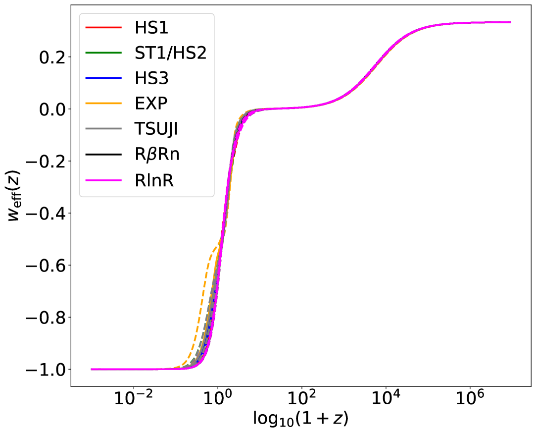
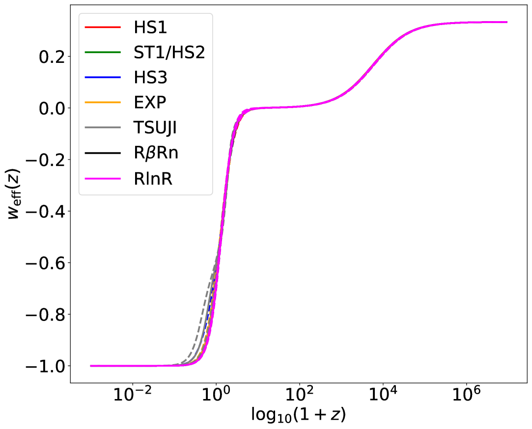
The evolution of the Universe, transitioning through radiation-dominated, matter- dominated to final de-Sitter phase (in distant future), is characterized by the total equation-of-state (EoS) parameter () as a function of redshift, exhibiting values , and in these respective phases. Whereas for the current accelerated expansion phase we expect (at ) or more appropriately we should explore for this purpose. From Fig. 12 we can see that all the models considered in present work are able to reproduce aforementioned three phases of the evolution of the Universe, both for the data sets without and with SH0ES prior on . Also the model predicted values of (i.e. at ) are reasonably close to 0.7, as can be seen from the eighth column of Tables LABEL:resultstable_Pal and LABEL:resultsH0table_Pal, for data sets without and with SH0ES prior, respectively.
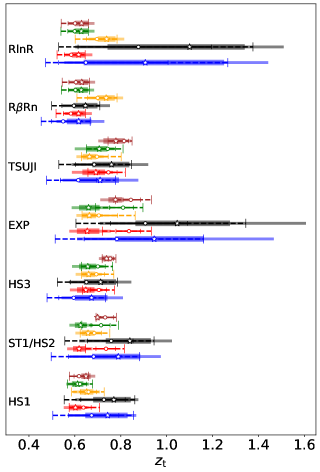
Now let us explore the nature of late-time accelerated expansion, and prediction for the distant future. The relevant derived quantities that describe the current accelerated expansion of the Universe is the deceleration parameter (), defined as , indicates whether and when the expansion of the Universe experiences acceleration () or deceleration (). Many measurements of , which are independent of any specific cosmological model (in addition to model- dependent ones), indicate that and [98, 99]. Here, is referred to as the transition redshift, signifying the redshift at which the Universe transitioned from a phase of decelerated expansion to the current accelerated expansion. As can be seen from Fig. 13 and sixth column of Tables LABEL:resultstable_Pal and LABEL:resultsH0table_Pal, that the model predicted values of transition redshift are mostly within the range , and these values are in agreement with model independent estimates from [98] and [99].
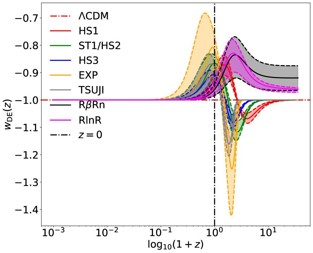
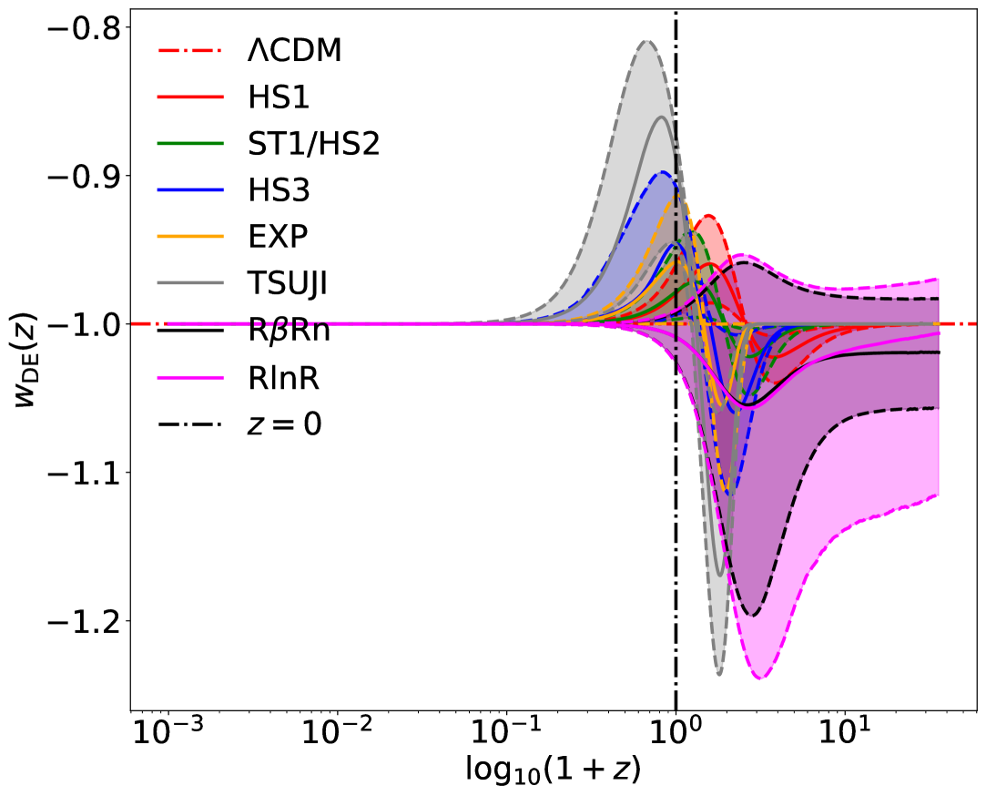
In Fig. 14 we have plotted the evolution of (define in Eq. 22 by the name ) for (past) to distant future , from the constraints on models from data sets SCBHii and SCBHii. These curves, for all the models, are supposed to converge to in the distant past for successfully producing matter dominated epoch, the trends for which are clearly visible in Fig. 14. Except for the models RRn and RlnR, corresponding to data set SCBHii, for all models we can observe the crossing of phantom-divide line () by model predicted , in recent past from the so-called phantom regime () to the so-called quintessence regime (). Also can we see that all the models are converging to a value of in distant future, that is, successfully reproducing the de-Sitter phase of the Universe.
8 Concluding Remarks
With SNIa data from Pantheonplus compilation, CC data, BAO data, H ii starburst galaxies data, distance priors of the CMBR and local measurement of , we have investigated seven models in the Palatini formalism, namely, the Hu–Sawicki model (), the Starobisnky model (), the exponential model, the Tsujikawa model, , and . To address the so-called Hubble tension we included data set combinations without vis-a-vis with SH0ES prior on . Although in their original forms, these models appear unrelated to the standard CDM model, but when re-parameterized in terms of deviation parameter (), it becomes apparent that all these models reduce to the CDM model with . Therefore, all these models are characterized with three parameters: (), except when studied with CMB data, we need one more parameter, namely, .
In most cases, the Planck constrained value of matter density at present epoch, , lie within limits of the model predicted median values of or vice-versa, both for the data sets with or without SH0ES prior on . Same is true for vis-a-vis the model predicted median values of , but for the data sets without SH0ES prior. For the data sets with SH0ES prior, the SH0ES measured value fall within limits of the model predicted median values of but on the higher side, when CMB data is not included. Whereas with inclusion of CMB data, the tensions between model predicted values of and enhance, as for these cases, even with SH0ES prior, the values are more nearer to .
The derived parameters essential for characterizing the accelerated expansion of the Universe, namely, , , and , estimated in this study, are closer to and compatible with their estimations from cosmological model-independent methods by earlier studies. This work predicts that the transition from decelerated phase of expansion into accelerated phase of expansion happened around , according to almost all the models investigated here. Additionally, the model predicted values of fall in the quintessential region, having recently transitioned from the phantom region, with exception of a few cases.
Our analysis unveils instances across all examined models where the deviation parameter significantly differs from zero. It is noteworthy that these instances also coincide with situations where analyses based on AIC, DIC, and/or BIC strongly favor the models over the CDM model. Previous studies have generally shown weak or positive support for models based on AIC, DIC, and/or BIC. However, this work demonstrates cases of (very) strong support for models.
With cases of (very) strong support for models, non-zero supported by AIC, DIC and/or BIC, and the quantities , , and being compatible with their model-independent predicted values, we find that the cosmological data analyzed in this study do not yet warrant dismissing the models in Palatini formalism. Instead, our study advocates for further exploration of these models within the Palatini formalism as plausible contenders for explaining the evolutionary trajectory of the Universe, with observed cosmological data sets to come in the future.
Data Availability
The observed cosmological data such as SNIa, CC, BAO, H ii starburst galaxies, CMB distance priors, and local measurement of are publicly available — the references to which are cited in the text. The simulated data sets generated in this work are available from the corresponding author upon reasonable request.
Acknowledgements
I would like to thank HoD, Dept. of Comp. Sc., RKMVERI, for providing computational
facilities. I would also like to thank Dr. Abhijit Bandyopadhyay for helpful discussions.
References
References
- [1] Supernova Cosmology Project collaboration, Discovery of a supernova explosion at half the age of the Universe and its cosmological implications, Nature 391 (1998) 51 [astro-ph/9712212].
- [2] Supernova Cosmology Project collaboration, Measurements of and from 42 high redshift supernovae, Astrophys. J. 517 (1999) 565 [astro-ph/9812133].
- [3] Supernova Search Team collaboration, The High Z supernova search: Measuring cosmic deceleration and global curvature of the universe using type Ia supernovae, Astrophys. J. 507 (1998) 46 [astro-ph/9805200].
- [4] Supernova Search Team collaboration, Observational evidence from supernovae for an accelerating universe and a cosmological constant, Astron. J. 116 (1998) 1009 [astro-ph/9805201].
- [5] SDSS collaboration, Detection of the Baryon Acoustic Peak in the Large-Scale Correlation Function of SDSS Luminous Red Galaxies, Astrophys. J. 633 (2005) 560 [astro-ph/0501171].
- [6] W.J. Percival et al., Measuring the matter density using baryon oscillations in the SDSS, Astrophys. J. 657 (2007) 51 [astro-ph/0608635].
- [7] WMAP collaboration, Wilkinson Microwave Anisotropy Probe (WMAP) three year results: implications for cosmology, Astrophys. J. Suppl. 170 (2007) 377 [astro-ph/0603449].
- [8] WMAP collaboration, Five-Year Wilkinson Microwave Anisotropy Probe (WMAP) Observations: Data Processing, Sky Maps, and Basic Results, Astrophys. J. Suppl. 180 (2009) 225 [0803.0732].
- [9] Planck collaboration, Planck 2013 results. XVI. Cosmological parameters, Astron. Astrophys. 571 (2014) A16 [1303.5076].
- [10] Planck collaboration, Planck 2015 results. XIII. Cosmological parameters, Astron. Astrophys. 594 (2016) A13 [1502.01589].
- [11] 2dFGRS collaboration, The 2dF Galaxy Redshift Survey: Power-spectrum analysis of the final dataset and cosmological implications, Mon. Not. Roy. Astron. Soc. 362 (2005) 505 [astro-ph/0501174].
- [12] W.J. Percival et al., The shape of the SDSS DR5 galaxy power spectrum, Astrophys. J. 657 (2007) 645 [astro-ph/0608636].
- [13] I. Zlatev, L.-M. Wang and P.J. Steinhardt, Quintessence, cosmic coincidence, and the cosmological constant, Phys. Rev. Lett. 82 (1999) 896 [astro-ph/9807002].
- [14] J. Martin, Everything You Always Wanted To Know About The Cosmological Constant Problem (But Were Afraid To Ask), Comptes Rendus Physique 13 (2012) 566 [1205.3365].
- [15] M. Chevallier and D. Polarski, Accelerating universes with scaling dark matter, Int. J. Mod. Phys. D 10 (2001) 213 [gr-qc/0009008].
- [16] E.V. Linder, Exploring the expansion history of the universe, Phys. Rev. Lett. 90 (2003) 091301 [astro-ph/0208512].
- [17] W. Yang, E. Di Valentino, S. Pan, Y. Wu and J. Lu, Dynamical dark energy after Planck CMB final release and tension, Mon. Not. Roy. Astron. Soc. 501 (2021) 5845 [2101.02168].
- [18] S. Tsujikawa, Quintessence: A Review, Class. Quant. Grav. 30 (2013) 214003 [1304.1961].
- [19] C. Armendariz-Picon, V.F. Mukhanov and P.J. Steinhardt, Essentials of k essence, Phys. Rev. D 63 (2001) 103510 [astro-ph/0006373].
- [20] J.F. Pascual-Sanchez, Cosmic acceleration: Inhomogeneity versus vacuum energy, Mod. Phys. Lett. A 14 (1999) 1539 [gr-qc/9905063].
- [21] M.-N. Celerier, Do we really see a cosmological constant in the supernovae data?, Astron. Astrophys. 353 (2000) 63 [astro-ph/9907206].
- [22] A. Krasinski, Inhomogeneous cosmological models, Cambridge Univ. Press, Cambridge, UK (3, 2011).
- [23] K. Bolejko, M.-N. Celerier and A. Krasinski, Inhomogeneous cosmological models: Exact solutions and their applications, Class. Quant. Grav. 28 (2011) 164002 [1102.1449].
- [24] V. Marra and A. Notari, Observational constraints on inhomogeneous cosmological models without dark energy, Class. Quant. Grav. 28 (2011) 164004 [1102.1015].
- [25] K. Enqvist and T. Mattsson, The effect of inhomogeneous expansion on the supernova observations, JCAP 02 (2007) 019 [astro-ph/0609120].
- [26] K. Enqvist, Lemaitre-Tolman-Bondi model and accelerating expansion, Gen. Rel. Grav. 40 (2008) 451 [0709.2044].
- [27] B. Santos, M. Campista, J. Santos and J.S. Alcaniz, Cosmology with Hu-Sawicki gravity in Palatini Formalism, Astron. Astrophys. 548 (2012) A31 [1207.2478].
- [28] M. Campista, B. Santos, J. Santos and J.S. Alcaniz, Cosmological Consequences of Exponential Gravity in Palatini Formalism, Phys. Lett. B 699 (2011) 320 [1012.3943].
- [29] M. Amarzguioui, O. Elgaroy, D.F. Mota and T. Multamaki, Cosmological constraints on f(r) gravity theories within the palatini approach, Astron. Astrophys. 454 (2006) 707 [astro-ph/0510519].
- [30] S. Fay, R. Tavakol and S. Tsujikawa, f(R) gravity theories in Palatini formalism: Cosmological dynamics and observational constraints, Phys. Rev. D 75 (2007) 063509 [astro-ph/0701479].
- [31] F.C. Carvalho, E.M. Santos, J.S. Alcaniz and J. Santos, Cosmological Constraints from Hubble Parameter on f(R) Cosmologies, JCAP 09 (2008) 008 [0804.2878].
- [32] J. Santos, J.S. Alcaniz, F.C. Carvalho and N. Pires, Latest supernovae constraints on f(R) cosmologies, Phys. Lett. B 669 (2008) 14 [0808.4152].
- [33] W. Hu and I. Sawicki, Models of f(R) Cosmic Acceleration that Evade Solar-System Tests, Phys. Rev. D 76 (2007) 064004 [0705.1158].
- [34] S. Basilakos, S. Nesseris and L. Perivolaropoulos, Observational constraints on viable f(R) parametrizations with geometrical and dynamical probes, Phys. Rev. D 87 (2013) 123529 [1302.6051].
- [35] K. Ravi, A. Chatterjee, B. Jana and A. Bandyopadhyay, Investigating the accelerated expansion of the Universe through updated constraints on viable models within the metric formalism, Mon. Not. Roy. Astron. Soc. 527 (2024) 7626 [2306.12585].
- [36] A.A. Starobinsky, Disappearing cosmological constant in f(R) gravity, JETP Lett. 86 (2007) 157 [0706.2041].
- [37] G. Cognola, E. Elizalde, S. Nojiri, S.D. Odintsov, L. Sebastiani and S. Zerbini, A Class of viable modified f(R) gravities describing inflation and the onset of accelerated expansion, Phys. Rev. D 77 (2008) 046009 [0712.4017].
- [38] E.V. Linder, Exponential Gravity, Phys. Rev. D 80 (2009) 123528 [0905.2962].
- [39] Y. Chen, C.-Q. Geng, C.-C. Lee, L.-W. Luo and Z.-H. Zhu, Constraints on the exponential model from latest Hubble parameter measurements, Phys. Rev. D 91 (2015) 044019 [1407.4303].
- [40] S.D. Odintsov, D. Sáez-Chillón Gómez and G.S. Sharov, Is exponential gravity a viable description for the whole cosmological history?, Eur. Phys. J. C 77 (2017) 862 [1709.06800].
- [41] M. Leizerovich, L. Kraiselburd, S.J. Landau and C.G. Scóccola, Testing f(R) gravity models with quasar x-ray and UV fluxes, Phys. Rev. D 105 (2022) 103526 [2112.01492].
- [42] S. Tsujikawa, Observational signatures of dark energy models that satisfy cosmological and local gravity constraints, Phys. Rev. D 77 (2008) 023507 [0709.1391].
- [43] M.M. Phillips, The absolute magnitudes of Type IA supernovae, Astrophys. J. Lett. 413 (1993) L105.
- [44] D. Scolnic et al., The Pantheon+ Analysis: The Full Data Set and Light-curve Release, Astrophys. J. 938 (2022) 113 [2112.03863].
- [45] Pan-STARRS1 collaboration, The Complete Light-curve Sample of Spectroscopically Confirmed SNe Ia from Pan-STARRS1 and Cosmological Constraints from the Combined Pantheon Sample, Astrophys. J. 859 (2018) 101 [1710.00845].
- [46] SNLS collaboration, Supernova Constraints and Systematic Uncertainties from the First 3 Years of the Supernova Legacy Survey, Astrophys. J. Suppl. 192 (2011) 1 [1104.1443].
- [47] R. Jimenez and A. Loeb, Constraining cosmological parameters based on relative galaxy ages, Astrophys. J. 573 (2002) 37 [astro-ph/0106145].
- [48] J.-J. Wei, Model-independent Curvature Determination from Gravitational-Wave Standard Sirens and Cosmic Chronometers, Astrophys. J. 868 (2018) 29 [1806.09781].
- [49] J. Simon, L. Verde and R. Jimenez, Constraints on the redshift dependence of the dark energy potential, Phys. Rev. D 71 (2005) 123001 [astro-ph/0412269].
- [50] M. Moresco, L. Pozzetti, A. Cimatti, R. Jimenez, C. Maraston, L. Verde et al., A 6% measurement of the Hubble parameter at : direct evidence of the epoch of cosmic re-acceleration, JCAP 05 (2016) 014 [1601.01701].
- [51] M. Moresco, Raising the bar: new constraints on the Hubble parameter with cosmic chronometers at z 2, Mon. Not. Roy. Astron. Soc. 450 (2015) L16 [1503.01116].
- [52] C. Zhang, H. Zhang, S. Yuan, T.-J. Zhang and Y.-C. Sun, Four new observational data from luminous red galaxies in the Sloan Digital Sky Survey data release seven, Res. Astron. Astrophys. 14 (2014) 1221 [1207.4541].
- [53] D. Stern, R. Jimenez, L. Verde, M. Kamionkowski and S.A. Stanford, Cosmic Chronometers: Constraining the Equation of State of Dark Energy. I: H(z) Measurements, JCAP 02 (2010) 008 [0907.3149].
- [54] M. Moresco et al., Improved constraints on the expansion rate of the Universe up to z~1.1 from the spectroscopic evolution of cosmic chronometers, JCAP 08 (2012) 006 [1201.3609].
- [55] A.L. Ratsimbazafy, S.I. Loubser, S.M. Crawford, C.M. Cress, B.A. Bassett, R.C. Nichol et al., Age-dating Luminous Red Galaxies observed with the Southern African Large Telescope, Mon. Not. Roy. Astron. Soc. 467 (2017) 3239 [1702.00418].
- [56] N. Borghi, M. Moresco and A. Cimatti, Toward a Better Understanding of Cosmic Chronometers: A New Measurement of H(z) at z 0.7, Astrophys. J. Lett. 928 (2022) L4 [2110.04304].
- [57] Planck collaboration, Planck 2018 results. VI. Cosmological parameters, Astron. Astrophys. 641 (2020) A6 [1807.06209].
- [58] A.G. Riess et al., A Comprehensive Measurement of the Local Value of the Hubble Constant with 1 km s-1 Mpc-1 Uncertainty from the Hubble Space Telescope and the SH0ES Team, Astrophys. J. Lett. 934 (2022) L7 [2112.04510].
- [59] A.L. González-Morán, R. Chávez, E. Terlevich, R. Terlevich, D. Fernández-Arenas, F. Bresolin et al., Independent cosmological constraints from high-z H ii galaxies: new results from VLT-KMOS data, Mon. Not. Roy. Astron. Soc. 505 (2021) 1441 [2105.04025].
- [60] D.K. Erb, C.C. Steidel, A.E. Shapley, M. Pettini, N.A. Reddy and K.L. Adelberger, The Stellar, Gas and Dynamical Masses of Star-Forming Galaxies at z 2, Astrophys. J. 646 (2006) 107 [astro-ph/0604041].
- [61] M.V. Maseda et al., The Nature of Extreme Emission Line Galaxies at z=1-2: Kinematics and Metallicities from Near-Infrared Spectroscopy, Astrophys. J. 791 (2014) 17 [1406.3351].
- [62] D. Masters et al., Physical Properties of Emission-Line Galaxies at z ~ 2 from Near-Infrared Spectroscopy with Magellan FIRE, Astrophys. J. 785 (2014) 153 [1402.0510].
- [63] A.L. González-Morán, R. Chávez, R. Terlevich, E. Terlevich, F. Bresolin, D. Fernández-Arenas et al., Independent cosmological constraints from high-z H ii galaxies, Mon. Not. Roy. Astron. Soc. 487 (2019) 4669 [1906.02195].
- [64] R. Chávez, M. Plionis, S. Basilakos, R. Terlevich, E. Terlevich, J. Melnick et al., Constraining the dark energy equation of state with H galaxies, Mon. Not. Roy. Astron. Soc. 462 (2016) 2431 [1607.06458].
- [65] W. Hu and N. Sugiyama, Small scale cosmological perturbations: An Analytic approach, Astrophys. J. 471 (1996) 542 [astro-ph/9510117].
- [66] D.J. Eisenstein and W. Hu, Baryonic features in the matter transfer function, Astrophys. J. 496 (1998) 605 [astro-ph/9709112].
- [67] F. Beutler, C. Blake, M. Colless, D.H. Jones, L. Staveley-Smith, L. Campbell et al., The 6dF Galaxy Survey: Baryon Acoustic Oscillations and the Local Hubble Constant, Mon. Not. Roy. Astron. Soc. 416 (2011) 3017 [1106.3366].
- [68] SDSS collaboration, Baryon Acoustic Oscillations in the Sloan Digital Sky Survey Data Release 7 Galaxy Sample, Mon. Not. Roy. Astron. Soc. 401 (2010) 2148 [0907.1660].
- [69] N. Padmanabhan, X. Xu, D.J. Eisenstein, R. Scalzo, A.J. Cuesta, K.T. Mehta et al., A 2 per cent distance to =0.35 by reconstructing baryon acoustic oscillations - I. Methods and application to the Sloan Digital Sky Survey, Mon. Not. Roy. Astron. Soc. 427 (2012) 2132 [1202.0090].
- [70] R. Tojeiro et al., The clustering of galaxies in the SDSS-III Baryon Oscillation Spectroscopic Survey: galaxy clustering measurements in the low redshift sample of Data Release 11, Mon. Not. Roy. Astron. Soc. 440 (2014) 2222 [1401.1768].
- [71] L. Anderson et al., The clustering of galaxies in the SDSS-III Baryon Oscillation Spectroscopic Survey: Baryon Acoustic Oscillations in the Data Release 9 Spectroscopic Galaxy Sample, Mon. Not. Roy. Astron. Soc. 427 (2013) 3435 [1203.6594].
- [72] J.E. Bautista et al., The SDSS-IV extended Baryon Oscillation Spectroscopic Survey: Baryon Acoustic Oscillations at redshift of 0.72 with the DR14 Luminous Red Galaxy Sample, Astrophys. J. 863 (2018) 110 [1712.08064].
- [73] H.-J. Seo et al., Acoustic scale from the angular power spectra of SDSS-III DR8 photometric luminous galaxies, Astrophys. J. 761 (2012) 13 [1201.2172].
- [74] S. Sridhar, Y.-S. Song, A.J. Ross, R. Zhou, J.A. Newman, C.-H. Chuang et al., Clustering of LRGs in the DECaLS DR8 Footprint: Distance Constraints from Baryon Acoustic Oscillations Using Photometric Redshifts, Astrophys. J. 904 (2020) 69 [2005.13126].
- [75] V. de Sainte Agathe et al., Baryon acoustic oscillations at z = 2.34 from the correlations of Ly absorption in eBOSS DR14, Astron. Astrophys. 629 (2019) A85 [1904.03400].
- [76] P. Carter, F. Beutler, W.J. Percival, C. Blake, J. Koda and A.J. Ross, Low Redshift Baryon Acoustic Oscillation Measurement from the Reconstructed 6-degree Field Galaxy Survey, Mon. Not. Roy. Astron. Soc. 481 (2018) 2371 [1803.01746].
- [77] A.J. Ross, L. Samushia, C. Howlett, W.J. Percival, A. Burden and M. Manera, The clustering of the SDSS DR7 main Galaxy sample – I. A 4 per cent distance measure at , Mon. Not. Roy. Astron. Soc. 449 (2015) 835 [1409.3242].
- [78] E.A. Kazin et al., The WiggleZ Dark Energy Survey: improved distance measurements to z = 1 with reconstruction of the baryonic acoustic feature, Mon. Not. Roy. Astron. Soc. 441 (2014) 3524 [1401.0358].
- [79] M. Ata et al., The clustering of the SDSS-IV extended Baryon Oscillation Spectroscopic Survey DR14 quasar sample: first measurement of baryon acoustic oscillations between redshift 0.8 and 2.2, Mon. Not. Roy. Astron. Soc. 473 (2018) 4773 [1705.06373].
- [80] DES collaboration, Dark Energy Survey Year 1 Results: Measurement of the Baryon Acoustic Oscillation scale in the distribution of galaxies to redshift 1, Mon. Not. Roy. Astron. Soc. 483 (2019) 4866 [1712.06209].
- [81] J.E. Bautista et al., Measurement of baryon acoustic oscillation correlations at with SDSS DR12 Ly-Forests, Astron. Astrophys. 603 (2017) A12 [1702.00176].
- [82] H. du Mas des Bourboux et al., Baryon acoustic oscillations from the complete SDSS-III Ly-quasar cross-correlation function at , Astron. Astrophys. 608 (2017) A130 [1708.02225].
- [83] BOSS collaboration, Quasar-Lyman Forest Cross-Correlation from BOSS DR11 : Baryon Acoustic Oscillations, JCAP 05 (2014) 027 [1311.1767].
- [84] BOSS collaboration, The clustering of galaxies in the completed SDSS-III Baryon Oscillation Spectroscopic Survey: cosmological analysis of the DR12 galaxy sample, Mon. Not. Roy. Astron. Soc. 470 (2017) 2617 [1607.03155].
- [85] J.E. Bautista et al., The Completed SDSS-IV extended Baryon Oscillation Spectroscopic Survey: measurement of the BAO and growth rate of structure of the luminous red galaxy sample from the anisotropic correlation function between redshifts 0.6 and 1, Mon. Not. Roy. Astron. Soc. 500 (2020) 736 [2007.08993].
- [86] R. Neveux et al., The completed SDSS-IV extended Baryon Oscillation Spectroscopic Survey: BAO and RSD measurements from the anisotropic power spectrum of the quasar sample between redshift 0.8 and 2.2, Mon. Not. Roy. Astron. Soc. 499 (2020) 210 [2007.08999].
- [87] A. Aizpuru, R. Arjona and S. Nesseris, Machine learning improved fits of the sound horizon at the baryon drag epoch, Phys. Rev. D 104 (2021) 043521 [2106.00428].
- [88] L. Chen, Q.-G. Huang and K. Wang, Distance Priors from Planck Final Release, JCAP 02 (2019) 028 [1808.05724].
- [89] N. Wogan, “numbalsoda.” https://github.com/Nicholaswogan/numbalsoda, 2022.
- [90] D. Foreman-Mackey, D.W. Hogg, D. Lang and J. Goodman, emcee: The MCMC Hammer, Publ. Astron. Soc. Pac. 125 (2013) 306 [1202.3665].
- [91] A. Lewis, GetDist: a Python package for analysing Monte Carlo samples, 1910.13970.
- [92] H. Akaike, A new look at the statistical model identification, IEEE Transactions on Automatic Control 19 (1974) 716.
- [93] G. Schwarz, Estimating the Dimension of a Model, The Annals of Statistics 6 (1978) 461 .
- [94] D.J. Spiegelhalter, N.G. Best, B.P. Carlin and A. Van Der Linde, Bayesian measures of model complexity and fit, Journal of the Royal Statistical Society: Series B (Statistical Methodology) 64 (2002) 583 [https://rss.onlinelibrary.wiley.com/doi/pdf/10.1111/1467-9868.00353].
- [95] A.R. Liddle, How many cosmological parameters?, Mon. Not. Roy. Astron. Soc. 351 (2004) L49 [astro-ph/0401198].
- [96] A.R. Liddle, Information criteria for astrophysical model selection, Mon. Not. Roy. Astron. Soc. 377 (2007) L74 [astro-ph/0701113].
- [97] K.P. Burnham and D.R. Anderson, Multimodel inference: Understanding aic and bic in model selection, Sociological Methods & Research 33 (2004) 261 [https://doi.org/10.1177/0049124104268644].
- [98] N. Rani, D. Jain, S. Mahajan, A. Mukherjee and N. Pires, Transition Redshift: New constraints from parametric and nonparametric methods, JCAP 12 (2015) 045 [1503.08543].
- [99] J.F. Jesus, R. Valentim, A.A. Escobal and S.H. Pereira, Gaussian Process Estimation of Transition Redshift, JCAP 04 (2020) 053 [1909.00090].