Weighted Particle-Based Optimization for Efficient Generalized Posterior Calibration

Abstract

In the realm of statistical learning, the increasing volume of accessible data and increasing model complexity necessitate robust methodologies. This paper explores two branches of robust Bayesian methods in response to this trend. The first is generalized Bayesian inference, which introduces a learning rate parameter to enhance robustness against model misspecifications. The second is Gibbs posterior inference, which formulates inferential problems using generic loss functions rather than probabilistic models. In such approaches, it is necessary to calibrate the spread of the posterior distribution by selecting a learning rate parameter. The study aims to enhance the generalized posterior calibration (GPC) algorithm proposed by Syring and Martin (2019) [Biometrika, Volume 106, Issue 2, pp. 479-486]. Their algorithm chooses the learning rate to achieve the nominal frequentist coverage probability, but it is computationally intensive because it requires repeated posterior simulations for bootstrap samples. We propose a more efficient version of the GPC inspired by sequential Monte Carlo (SMC) samplers. A target distribution with a different learning rate is evaluated without posterior simulation as in the reweighting step in SMC sampling. Thus, the proposed algorithm can reach the desired value within a few iterations. This improvement substantially reduces the computational cost of the GPC. Its efficacy is demonstrated through synthetic and real data applications.

1 Introduction

As the volume of accessible data and the complexity of models increase, the necessity for robustness in statistical learning intensifies. With this trend in mind, this study delves into two branches of robust Bayesian methods. First, it focuses on generalized Bayesian inference [1, 2]. Let $\mathcal{D}$ represent a dataset comprising $N$ independent samples, denoted by $\mathcal{D}=\left\{\mathcal{D}_{i}\right\}_{i=1}^{N}$. In conventional Bayesian inference, the posterior of a $K$-dimensional unknown parameter vector $\boldsymbol{\theta}$ combines a likelihood $p\left(\mathcal{D}|\boldsymbol{\theta}\right)$ with a prior $p\left(\boldsymbol{\theta}\right)$,

$$\pi\left(\boldsymbol{\theta}\right)\propto p\left(\mathcal{D}|\boldsymbol{\theta}\right)p\left(\boldsymbol{\theta}\right).$$

In contrast, generalized Bayesian inference introduces a generalized posterior by incorporating a learning rate $\eta\left(>0\right)$ (also termed a scaling parameter) alongside the likelihood, as follows:

$$\pi_{\eta}^{*}\left(\boldsymbol{\theta}\right)\propto p\left(\mathcal{D}|\boldsymbol{\theta}\right)^{\eta}p\left(\boldsymbol{\theta}\right).$$

By setting $\eta<1$, the posterior spread increases, rendering the inference robust against model misspecifications [3, 4, 5, 6]. The second category of robust Bayesian methods involves Gibbs posterior inference [7, 8, 9, 10, 11, 12]. This method formulates an inferential problem using a generic loss function $r_{i}\left(\boldsymbol{\theta};\mathcal{D}_{i}\right)$ rather than a probabilistic model. Under this approach, the posterior is expressed as

$$\pi_{\eta}^{*}\left(\boldsymbol{\theta}\right)\propto\exp\left\{-Nr\left(\boldsymbol{\theta};\mathcal{D}\right)\right\}^{\eta}p\left(\boldsymbol{\theta}\right),$$

where $r\left(\boldsymbol{\theta};\mathcal{D}\right)$ is an empirical risk function defined as

$$r\left(\boldsymbol{\theta};\mathcal{D}\right)=\frac{1}{N}\sum_{i=1}^{N}r_{i}\left(\boldsymbol{\theta};\mathcal{D}_{i}\right).$$

The algorithm proposed in the study can be applied to both approaches. In what follows, $q\left(\boldsymbol{\theta};\mathcal{D}\right)$ denotes either a likelihood $p\left(\mathcal{D}|\boldsymbol{\theta}\right)$ or pseudolikelihood $\exp\left\{-Nr\left(\boldsymbol{\theta};\mathcal{D}\right)\right\}$, with

$$\pi_{\eta}^{*}\left(\boldsymbol{\theta}\right)\propto q\left(\boldsymbol{\theta};\mathcal{D}\right)^{\eta}p\left(\boldsymbol{\theta}\right).$$ (1)

There are various methods for selecting $\eta$ [13, 14, 15, 16], each with distinct emphases. For a comparative analysis, refer to [17]. We aim to enhance the generalized posterior calibration (GPC) algorithm [16]. Within the GPC framework, the coverage probability for a particular $\eta$ value is assessed using bootstrap samples, and $\eta$ is chosen numerically to achieve the specified frequentist coverage probability. However, a significant drawback of the GPC method is its computational burden, as it necessiates repeated execution of a posterior simulator on bootstrap samples until convergence.

This paper proposes an improvement in the GPC that requires fewer of iterations. This algorithm is inspired by sequential Monte Carlo (SMC) samplers [18], exploiting the similarity between the learning rate in the GPC and an inverse temperature in SMC sampling. The target distribution with the current value of $\eta$ is approximated using weighted particles, as in SMC sampling. The particle approximation of the target distribution with a new value of $\eta$ is obtained without posterior simulation as in the reweighting step in SMC sampling. At least in theory, a desired value of $\eta$ is reached in a single step, although few iterations are required in practice due to the particle degeneracy problem.

A recent paper [19] proposed an algorithm that replaces an MCMC sampler with an SMC sampler. The algorithm proposed in this paper is different, in that it uses an MCMC sampler for posterior simulation and improves on the optimization procedure itself. SMC samplers are only applicable to relatively low-dimensional cases (say, with a sampling dimension less than 10). In contrast, there are MCMC samplers that are feasible for high-dimensional cases.

The subsequent sections are organized as follows. Section 2 describes the GPC algorithm and SMC samplers as background. Section 3 presents the newly proposed algorithm. Its application to synthetic and real data is illustrated in Section 4. Finally, Section 5 provides concluding remarks.

2 Background

2.1 Generalized posterior calibration

This section describes the generalized posterior calibration (GPC) [16] (Figure 1). $\mathcal{C}_{\alpha}^{\eta}\left(\mathcal{D}\right)$ denotes the generalized posterior $100\left(1-\alpha\right)\%$ credible set for $\boldsymbol{\theta}$ with $\eta$. The coverage probability is expressed as

$$c_{\alpha}\left(\eta|\mathbb{P}\right)=\mathbb{P}\left\{\boldsymbol{\theta}^{\dagger}\left(\eta\right)\in\mathcal{C}_{\alpha}^{\eta}\left(\mathcal{D}\right)\right\},$$

where $\boldsymbol{\theta}^{\dagger}\left(\eta\right)$ denotes the Kullback–Leibler minimizer obtained with $\eta$. Given that the true data distribution $\mathbb{P}$ is unknown, we substitute it with the empirical distribution $\mathbb{P}_{N}$,

$$c_{\alpha}\left(\eta|\mathbb{P}_{N}\right)=\mathbb{P}_{N}\left\{\hat{\boldsymbol{\theta}}\left(\eta\right)\in\mathcal{C}_{\alpha}^{\eta}\left(\mathcal{D}\right)\right\},$$

where $\hat{\boldsymbol{\theta}}\left(\eta\right)$ represents a point estimate of $\boldsymbol{\theta}$ obtained with $\eta$. However, direct evaluation of $c_{\alpha}\left(\eta|\mathbb{P}_{N}\right)$ is infeasible because it requires exhaustive enumeration of all $N^{N}$ possible with-replacement samples from $\mathcal{D}$. Consequently, we approximate $\mathbb{P}_{N}$ using a bootstrap method. With $B$ bootstrap samples $\left\{\breve{\mathcal{D}}^{\left[b\right]}\right\}_{b=1}^{B}$, the coverage probability is estimated as

$$\hat{c}_{\alpha}\left(\eta|\mathbb{P}_{N}\right)=\frac{1}{B}\sum_{b=1}^{B}\mathbb{I}\left\{\hat{\boldsymbol{\theta}}\left(\eta\right)\in\mathcal{C}_{\alpha}^{\eta}\left(\breve{\mathcal{D}}^{\left[b\right]}\right)\right\},$$

where $\mathbb{I}\left\{\cdot\right\}$ denotes the indicator function. $\eta$ is selected by solving $\hat{c}_{\alpha}\left(\eta|\mathbb{P}_{N}\right)=1-\alpha$ via a stochastic approximation [20]. At the $s$th iteration, a single step of stochastic approximation recursion is applied:

$$\eta_{s+1}\leftarrow\eta_{s}+\varsigma_{l}\left[\hat{c}_{\alpha}\left(\eta_{s}|\mathbb{P}_{N}\right)-\left(1-\alpha\right)\right],$$ (2)

where $\left\{\varsigma_{l}\right\}$ is a nonincreasing sequence such that $\sum_{l}\varsigma_{l}=\infty$ and $\sum_{l}\varsigma_{l}^{2}<\infty$. While [16] specified $\varsigma_{s}=s^{-0.51}$, we adopt a variant of Keston’s [21] rule (Figure 2), $\varsigma_{s}\left(l\right)=l^{-0.51}$, where $l$ increases by one only when there is a directional change in the trajectory of $\eta_{s}$ and $\hat{c}_{\alpha}\left(\eta_{s}|\mathbb{P}_{N}\right)<1$. This adaptation significantly reduces the convergence time.

Figure 1: Generalized posterior calibration

input:observed dataset $\mathcal{D}$, target kernel $\pi_{\eta}^{*}\left(\cdot\right)$, initial guess $\eta_{1}$, target credibility level $\alpha$, termination threshold $\epsilon$.

Generate $B$ bootstrap samples $\left\{\breve{\mathcal{D}}^{\left[b\right]}\right\}_{b=1}^{B}$ from $\mathcal{D}$.

Set $s\leftarrow 1$ and $l\leftarrow 1$.

while converge

   Compute $\hat{\boldsymbol{\theta}}$ with $\eta_{s}$.

   for $b=1,...,B$:

      Simulate $M$ posterior draws for $\breve{\mathcal{D}}^{\left[b\right]}$ using an MCMC

         sampler with $\eta_{s}$.

      Compute the credible set $\mathcal{C}_{\alpha}^{\eta_{s}}\left(\breve{\mathcal{D}}^{\left[b\right]}\right)$.

   end for

   Compute the coverage probability $\hat{c}_{\alpha}\left(\eta_{s}|\mathbb{P}_{N}\right)$.

   if $\left|\hat{c}_{\alpha}\left(\eta_{s}|\mathbb{P}_{N}\right)-\left(1-\alpha\right)\right|<\epsilon$:

      Set $\hat{\eta}\leftarrow\eta_{s}$.

      break

   else

      Set a new learning rate $\eta_{s+1}$ according to

         Figure 2 (GPC-SA) or Figure 3 (GPC-WP).

      Set $s\leftarrow s+1$.

   end if

end while

return: $\hat{\eta}$

Figure 2: A single step of stochastic approximation recursion with Keston’s rule

input: last three values $\left\{\eta_{i},\eta_{i-1},\eta_{i-2}\right\}$, current value $l$, empirical coverage probability $\hat{c}_{\alpha}\left(\eta_{i}|\mathbb{P}_{N}\right)$, credibility level $\alpha$

if $\left(\eta_{i-1}-\eta_{i-2}\right)\left(\eta_{i}-\eta_{i-1}\right)<0$ and $i>2$:

   $l\leftarrow l+1$.

end if

Set a new learning rate:

$$\eta_{i+1}\leftarrow\eta_{i}+l^{-0.51}\left[\hat{c}_{\alpha}\left(\eta_{i}|\mathbb{P}_{N}\right)-\left(1-\alpha\right)\right].$$

return: $\eta_{i+1}$, $l$

Note: $l$ is initialized to one at the beginning of the iterations.

2.2 Sequential Monte Carlo sampler

The following describles sequential Monte Carlo (SMC) samplers [18]. These algorithms repeatedly utilize importance sampling to generate sets of weighted particles $\left\{w^{\left[m\right]},\boldsymbol{\theta}^{\left[m\right]}\right\}_{m=1}^{M}$ that approximate a sequence of synthetic intermediate distributions $\left\{\pi_{t}\right\}_{t=0}^{T}$. Initially, the distribution $\pi_{0}$ corresponds to the prior, $\pi_{0}\left(\boldsymbol{\theta}\right)=p\left(\boldsymbol{\theta}\right)$, while the terminal distribution $\pi_{T}$ is the target distribution, i.e., the posterior, $\pi_{T}\left(\boldsymbol{\theta}\right)=p\left(\mathcal{D}|\boldsymbol{\theta}\right)p\left(\boldsymbol{\theta}\right)$. Each intermediate distribution is defined as a likelihood-tempered posterior:

$$\pi_{t}\left(\boldsymbol{\theta}\right)\propto p\left(\mathcal{D}|\boldsymbol{\theta}\right)^{\phi_{t}}p\left(\boldsymbol{\theta}\right),$$ (3)

where $\left\{\phi_{t}\right\}_{t=1}^{T}$ is an increasing sequence with $\phi_{0}=0$ and $\phi_{T}=1$. The parameter $\phi_{t}$ can be interpreted as the inverse temperature. We denote a sequence of auxiliary distributions as $\left\{\tilde{\pi}_{t}\right\}_{t=0}^{T}$ with

$$\tilde{\pi}_{t}\left(\boldsymbol{\theta}_{0:t}\right)=\pi_{t}\left(\boldsymbol{\theta}_{t}\right)\prod_{s=0}^{t-1}\mathcal{L}_{s}\left(\boldsymbol{\theta}_{s+1},\boldsymbol{\theta}_{s}\right),$$

where $\mathcal{L}_{t}\left(\cdot,\cdot\right)$ denotes a Markov kernel, also known as a backward kernel, which transitions backward from $\boldsymbol{\theta}_{t+1}$ to $\boldsymbol{\theta}_{t}$. Weighted particles $\left\{w_{t}^{\left[m\right]},\boldsymbol{\theta}_{t}^{\left[m\right]}\right\}_{m=1}^{M}$ are used to approximate $\tilde{\pi}_{t}$. These particles are moved via a Markov kernel $\mathcal{K}_{t}\left(\cdot,\cdot\right)$, termed a forward kernel. Let $\gamma_{t}\left(\boldsymbol{\theta}\right)$ denote the unnormalized posterior density with $\phi_{t}$,

$$\gamma_{t}\left(\boldsymbol{\theta}\right)=p\left(\mathcal{D}|\boldsymbol{\theta}\right)^{\phi_{t}}p\left(\boldsymbol{\theta}\right).$$

The unnormalized weights are expressed as follows:

$$W_{t}^{\left[m\right]}\propto\frac{\tilde{\pi}_{t}\left(\boldsymbol{\theta}_{t}^{\left[m\right]}\right)\prod_{s=1}^{t-1}\mathcal{L}_{s}\left(\boldsymbol{\theta}_{s+1}^{\left[m\right]},\boldsymbol{\theta}_{s}^{\left[m\right]}\right)}{\zeta_{1}\left(\boldsymbol{\theta}_{1}^{\left[m\right]}\right)\prod_{s^{\prime}=1}^{t-1}\mathcal{K}_{s^{\prime}}\left(\boldsymbol{\theta}_{s^{\prime}-1}^{\left[m\right]},\boldsymbol{\theta}_{s^{\prime}}^{\left[m\right]}\right)}.$$

Let $\widetilde{W}_{t}^{\left[m\right]}$ represent the unnormalized incremental weight, defined as:

$$\widetilde{W}_{t}^{\left[m\right]}=\frac{\gamma_{t}\left(\boldsymbol{\theta}_{t}^{\left[m\right]}\right)\mathcal{L}_{t-1}\left(\boldsymbol{\theta}_{t}^{\left[m\right]},\boldsymbol{\theta}_{t-1}^{\left[m\right]}\right)}{\gamma_{t-1}\left(\boldsymbol{\theta}_{t-1}^{\left[m\right]}\right)\mathcal{K}_{t}\left(\boldsymbol{\theta}_{t-1}^{\left[m\right]},\boldsymbol{\theta}_{t}^{\left[m\right]}\right)}.$$

Then, we have $W_{t}^{\left[m\right]}\propto\widetilde{W}_{t}^{\left[m\right]}W_{t-1}^{\left[m\right]}$.

When the forward kernel $\mathcal{K}_{t}$ is chosen as $\pi_{t}$-invariant, e.g., an MCMC kernel, this selection is deemed optimal because it minimizes the variance of the weights [18]. The backward kernel is formulated as:

$$\mathcal{L}_{t-1}\left(\boldsymbol{\theta}_{t}^{\left[m\right]},\boldsymbol{\theta}_{t-1}^{\left[m\right]}\right)=\frac{\pi_{t}\left(\boldsymbol{\theta}_{t-1}^{\left[m\right]}\right)\mathcal{K}_{t}\left(\boldsymbol{\theta}_{t-1}^{\left[m\right]},\boldsymbol{\theta}_{t}^{\left[m\right]}\right)}{\pi_{t}\left(\boldsymbol{\theta}_{t}^{\left[m\right]}\right)}.$$

With this specification, the unnormalized incremental weights simplify to:

$$\widetilde{W}_{t}^{\left[m\right]}=\frac{\gamma_{t}\left(\boldsymbol{\theta}_{t-1}^{\left[m\right]}\right)}{\gamma_{t-1}\left(\boldsymbol{\theta}_{t-1}^{\left[m\right]}\right)}=p\left(\mathcal{D}|\boldsymbol{\theta}_{t-1}^{\left[m\right]}\right)^{\phi_{t}-\phi_{t-1}}.$$

Thus, the unnormalized weights are updated as follows:

$$W_{t}^{\left[m\right]}=w_{t-1}^{\left[m\right]}p\left(\mathcal{D};\boldsymbol{\theta}_{t-1}^{\left[m\right]}\right){}^{\phi_{t}-\phi_{t-1}}.$$

The weights are normalized as:

$$w_{t}^{\left[m\right]}=W_{t}^{\left[m\right]}\left(\sum_{m^{\prime}=1}^{M}W_{t}^{\left[m^{\prime}\right]}\right)^{-1}.$$

Note that this reweighting step does not involve a re-evaluation of the likelihood $p\left(\mathcal{D}|\boldsymbol{\theta}_{t-1}^{\left[m\right]}\right)$.

As the difference in the consecutive temperatures increases, the variance of the weights is likely to increase and only a portion of the weights will be prominent, leading to the degeneration of the particle system. To address this problem, the quality of the particle approximation is monitored based on the effective sample size (ESS) [22], which captures the variance of the weights,

$$ESS_{t}=\frac{1}{\sum_{m=1}^{M}\left(w_{t}^{\left[m\right]}\right)^{2}}=\frac{\left(\sum_{m=1}^{M}W_{t-1}^{\left[m\right]}\widetilde{W}_{t}^{\left[m\right]}\right)^{2}}{\sum_{m=1}^{M}\left(W_{t-1}^{\left[m\right]}\widetilde{W}_{t}^{\left[m\right]}\right)^{2}}.$$

When the ESS is below a prespecified threshold $\overline{ESS}$, the weighted particles are resampled [23].

3 Proposed Algorithm

We propose a novel approach to find the best choice for the next learning rate $\eta_{s+1}$, which is called weighted particle-based optimization. The proposed approach is inspired by SMC samplers [18, 24]: the learning rate $\eta$ in the generalized/Gibbs posterior (1) and the inverse temperature in the likelihood-tempered posterior in SMC sampling (3) play similar roles in tempering the likelihood.

At the $s$th iteration, we generate pseudoposterior draws using an MCMC sampler with $\eta_{s}$. The posterior distribution with $\eta_{s}$ is approximated using a system of weighted particles, $\left\{w_{s}^{\left[b,m\right]},\boldsymbol{\theta}_{s}^{\left[b,m\right]}\right\}_{m=1}^{M}$, where $\sum_{m=1}^{M}w_{s}^{\left[b,m\right]}=1$ and each weight $w_{s}^{\left[b,m\right]}$ is proportional to the posterior densities evaluated at the corresponding posterior draw $\boldsymbol{\theta}_{s}^{\left[b,m\right]}$. A new learning rate $\eta^{\prime}$ is chosen using stochastic approximation recursion (Figure 2). As in the reweighting step in SMC sampling, the weights for a new guess $\eta^{\prime}$ are computed as follows:

$$\widetilde{W}_{s}^{\left[b,m\right]}=w_{s}^{\left[b,m\right]}q\left(\boldsymbol{\theta}_{s}^{\left[b,m\right]};\breve{\mathcal{D}}^{\left[b\right]}\right)^{\eta^{\prime}-\eta_{s}},$$

$$\widetilde{w_{s}}^{\left[b,m\right]}=\widetilde{W}_{s}^{\left[b,m\right]}\left(\sum_{m^{\prime}=1}^{M}\widetilde{W}_{s}^{\left[b,m^{\prime}\right]}\right)^{-1}.$$

Therefore, we can evaluate the credible set for the new value $\eta^{\prime}$ without re-evaluating the likelihood. The credible interval for each dimension is computed by sorting the particles and weights. Hereafter, we refer to the GPC with stochastic approximation optimization as the GPC-SA, while the GPC with weighted particle-based optimization is the GPC-WP.

The advantage of the GPC-WP over the GPC-SA is its low computational load. While the GPC-SA algorithm gradually approaches the optimal value , the proposed algorithm reaches it directly; at least in theory, no iteration is needed. However, as in SMC samplers, this algorithm can suffer from particle degeneracy. To maintain the quality of particle approximation, we terminate the stochastic approximation iteration if the minimum ESS is below a prespecified threshold, $minESS^{*}\left(\eta^{\prime};\eta_{s}\right)<\overline{ESS}$ with

$$minESS^{*}\left(\eta^{\prime};\eta_{s}\right)=\min\left\{ESS^{*\left[b\right]}\left(\eta^{\prime};\eta_{s}\right),\;b=1,...,B\right\},$$

$$ESS^{*\left[b\right]}\left(\eta^{\prime};\eta_{s}\right)=\frac{\left(\sum_{m=1}^{M}w_{s}^{\left[b,m\right]}q\left(\boldsymbol{\theta}_{s}^{\left[b,m\right]};\breve{\mathcal{D}}^{\left[b\right]}\right)^{\eta^{\prime}-\eta_{s}}\right)^{2}}{\sum_{m=1}^{M}\left(w_{s}^{\left[b,m\right]}p\left(\boldsymbol{\theta}_{s}^{\left[b,m\right]};\breve{\mathcal{D}}^{\left[b\right]}\right)^{\eta^{\prime}-\eta_{s}}\right)^{2}}.$$

In this paper, we choose $\overline{ESS}=0.25M$. Figure 3 summarizes the weighted particle-based optimization method, where parentheses are added to the subscripts of the learning rate, as in $\eta_{\left(u\right)}^{\prime}$, to distinguish it from the index related to the GPC iterations. $\iota$ denotes a flag for termination of the GPC algorithm: $\iota$ takes the value 1 if a calibrated value is found and 0 otherwise.

Figure 3: Weighted particle-based optimization

input: current learning rate $\eta_{s}$, current weighted particles $\left\{w_{s}^{\left[b,m\right]},\boldsymbol{\theta}_{s}^{\left[b,m\right]}\right\}_{m=1}^{M}$, resampling threshold $\overline{ESS}$, termination threshold $\epsilon$.

Set $u\leftarrow 1$, $l\leftarrow 1$, and $\iota\leftarrow 0$.

while not converged:

   Set a new learning rate $\eta_{\left(u\right)}^{\prime}$ using Algorithm 2.

   Compute the posterior estimate $\hat{\boldsymbol{\theta}}$ with $\eta_{\left(u\right)}^{\prime}$

   for $b=1,...,B$:

      Compute the unnormalized weights under $\eta_{\left(u\right)}^{\prime}$:

$$\widetilde{W}^{\left[b,m\right]}\leftarrow w_{s}^{\left[b,m\right]}q\left(\boldsymbol{\theta}_{s}^{\left[b,m\right]};\breve{\mathcal{D}}^{\left[b\right]}\right)^{\eta_{\left(u\right)}^{\prime}-\eta_{s}}$$

.

      Normalize the weights:

$$\widetilde{w}^{\left[b,m\right]}\leftarrow\widetilde{W}^{\left[b,m\right]}\left(\sum_{m^{\prime}=1}^{M}\widetilde{W}^{\left[b,m^{\prime}\right]}\right)^{-1}.$$

      Compute the credible set $\mathcal{C}_{\alpha}^{\eta_{\left(u\right)}^{\prime}}\left(\breve{\mathcal{D}}^{\left[b\right]}\right)$.

   end for

   if $\left|\hat{c}_{\alpha}\left(\eta_{\left(u\right)}^{\prime}|\mathbb{P}_{N}\right)-\left(1-\alpha\right)\right|<\epsilon$ and

         $minESS^{*}\left(\eta_{\left(u\right)}^{\prime};\eta_{s}\right)\geq\overline{ESS}$ then:

      A calibrated value has been reached; terminate GPC:

      $\hat{\eta}\leftarrow\eta_{\left(u\right)}^{\prime}$ and $\iota\leftarrow 1$.

   else if $minESS^{*}\left(\eta_{\left(u\right)}^{\prime};\eta_{s}\right)<\overline{ESS}$ then:

      Set the next value and continue GPC:

      $\eta_{s+1}\leftarrow\eta_{\left(u\right)}^{\prime}$.

      break

   else:

      Set $u\leftarrow u+1$.

   end if

end while

return: $\hat{\eta}$ or $\eta_{s+1}$, as well as $\iota$

4 Application

4.1 Misspecified linear regression

We considered a misspecified linear regression with synthetic data. The model to be estimated was specified as a homoskedastic linear regression:

$$y_{i}=\boldsymbol{\beta}^{\top}\boldsymbol{x}_{i}+\varepsilon_{i},\quad\varepsilon_{i}\sim\mathcal{N}\left(0,\sigma^{2}\right),$$

where $\boldsymbol{x}_{i}=\left(1,x_{1,i},x_{2,i},x_{3,i}\right)^{\top}$. The true data generation process, which was borrowed from Section 5.2 of [17] (Degree 2), had heteroskedastic errors depending on the first covariates:

$$y_{i}=\boldsymbol{\beta}^{\top}\boldsymbol{x}_{i}+\varepsilon_{i},\quad\varepsilon_{i}\sim\mathcal{N}\left(0,\sigma_{i}^{2}\right),$$

where $\sigma_{i}^{2}$ is 0.05 if $x_{1,i}<\xi_{0.05}$, 0.25 if $\xi_{0.05}\leq x_{1,i}\leq\xi_{0.95}$, and 1 if $\xi_{0.95}<x_{1,i}$; $\xi_{0.05}$ and $\xi_{0.95}$ denote the $5$th and 95th sample percentiles of $\left\{x_{1,1},,...,x_{1,N}\right\}$; and $\boldsymbol{\beta}=\left(\beta_{1},\beta_{2},\beta_{3},\beta_{4}\right)^{\top}=\left(1,1,2,-1\right)^{\top}$. Three sample sizes $N\in\left\{100,200,400\right\}$ were examined.

Posterior simulations were conducted using a Gibbs sampler. The unknown parameters $\boldsymbol{\theta}=\left(\boldsymbol{\beta}^{\top},\sigma^{2}\right)^{\top}$ were inferred using a normal prior, $\boldsymbol{\beta}\sim\mathcal{N}\left(\boldsymbol{0}_{4},\varsigma^{2}\boldsymbol{I}_{4}\right)$, and an inverse gamma prior, $\sigma^{2}\sim\mathcal{IG}\left(\varrho_{1},\varrho_{2}\right)$, where $\varsigma^{2}$, $\varrho_{1}$, and $\varrho_{2}$ are hyperparameters; $\mathcal{IG}\left(a,b\right)$ denotes an inverse gamma distribution with shape parameter $a$ and rate parameter $b$. The hyperparameters for $\sigma^{2}$ were set as $\left(\varrho_{1},\varrho_{2}\right)=\left(1,0.025\right)$. While [17] specified $\varsigma^{2}=\sigma^{2}$, $\boldsymbol{\beta}\sim\mathcal{N}\left(\boldsymbol{0}_{4},\sigma^{2}\boldsymbol{I}_{4}\right)$, our prior of $\boldsymbol{\beta}$ was independent of $\sigma^{2}$, $\varsigma^{2}=100$. Consequently, the resulting posterior was more general and computationally expensive because the inverse matrix had to be computed repeatedly.

We chose $\alpha=0.05$: the calibration target was the 95% credible set. Five hundred bootstrap samples were generated, so $B=500$. The stopping criterion was $\epsilon=0.005$. All the simulations began with $\eta=1$. The programs were executed on MATLAB (R2023b) on an Ubuntu desktop (22.04.4 LTS) running on an AMD Ryzen Threadripper 3990X 2.9 GHz 64-core processor. The computations using different bootstrap samples were parallelized.

We applied the two algorithms to 200 synthetic datasets. As shown in Table 1, both algorithms effectively achieved the target credibility level. Figure 4 compares the computational costs of the algorithms. The panels in the left column report the wall clock time in seconds. The median computation for the GPC-WP was approximately 25-30% faster than that of the GPC-SA. The improvement in the computational efficiency was due to the smaller number of iterations, as shown in the panels in the right column. While the GPC-SA needed approximately nine iterations, the GPC-WP converged within two or three iterations in most cases. The reason why the GPC-WP was not as fast as the GPC-SA in terms of the number of iterations was that it took more time to obtain the next learning rates. Nevertheless, this additional computational cost was outweighed by the gain from reducing the number of iterations.

Table 1: Coverage probability

$N$	Coverage probability (%)
	GPC-SA	GPC-WP
100	96.0	95.0
200	96.0	95.5
400	95.5	94.0

Note: The coverage probability of the ground truth is evaluated based on 200 synthetic datasets.

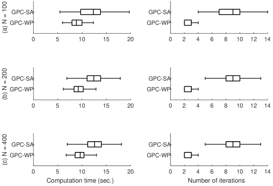
Figure 4: Comparison of the computational cost

Note: The boxplot displays the distribution of computation time (in seconds) for 200 synthetic datasets.

4.2 Support vector machine

We applied the proposed algorithm to estimate a support vector machine with real data, following Section 5 of [16]. The outcome is binary, $y_{i}\in\left\{-1,1\right\}$, and the feature vector is composed of an intercept and $K-1$ covariates, $\boldsymbol{x}_{i}=\left(1,x_{1,i},...,x_{K-1,i}\right)^{\top}$. Define $\boldsymbol{y}=\left(y_{1},...,y_{N}\right)^{\top}$ and $\boldsymbol{X}=\left(\boldsymbol{x}_{1},...,\boldsymbol{x}_{N}\right)^{\top}$. Estimating the support vector classifier is represented as the problem of minimizing the following empirical risk function:

$$r\left(\boldsymbol{\theta}\right)=\frac{1}{N}\sum_{i=1}^{N}2\max\left(0,1-y_{i}\boldsymbol{\theta}^{\top}\boldsymbol{x}_{i}\right),$$

where $\boldsymbol{\theta}\in\mathbb{R}^{K}$ is a vector of unknown parameters. We assigned an independent Laplace-type prior to $\boldsymbol{\theta}$. Then, the log pseudoposterior is represented as

$$\pi_{\eta}^{*}\left(\boldsymbol{\theta}\right)\propto-\eta\sum_{i=1}^{N}2\max\left(0,1-y_{i}\boldsymbol{x}_{i}^{\top}\boldsymbol{\theta}\right)-\nu^{-1}\sum_{k=1}^{K}\left|\frac{\theta_{k}}{\sigma_{k}}\right|,$$

where $\sigma_{k}$ denotes the standard deviation of the $k$th predictor $x_{k,1},...,x_{k,N}$ with $\sigma_{1}=1$ and $\nu\left(>0\right)$ is a hyperparameter. We chose $\nu=10$. This model was inferred for the South African Heart Disease dataset as in Section 4.4.2 of [25], with $N=462$ and $K=8$. For the posterior simulation, we modified a Gibbs sampler of [26] by incorporating $\eta$.

The two algorithms were executed 50 times using different random seeds. For every execution, both algorithms reached $\eta\approx 0.09$, which is in agreement with [16]. Figure 5 displays the computation time and number of iterations. The median computation time for the GPC-SA was 201.7 seconds, while that for the GPC-WP was 124.4 seconds (38.3% faster). The median required number of iterations for the GPC-SA was 7, while that for the GPC-WP was 4.

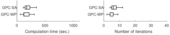
Figure 5: Comparison of the computational cost

Note: The boxplot displays the distribution of computation time (in seconds) for 50 runs with different random seeds.

5 Conclusion

In this paper, we explored two robust Bayesian methods: generalized Bayesian inference and Gibbs posterior inference. These methods offer robustness against model misspecifications by introducing learning rate parameters and formulating inferential problems using generic loss functions. Central to these approaches is the calibration of the posterior distribution spread through the selection of an appropriate learning rate parameter. Building upon the GPC algorithm proposed by [16], we introduced a more efficient version inspired by SMC samplers. Our proposed algorithm evaluates the coverage probability with a different learning rate without the need for repeated posterior simulations, substantially reducing the computational costs while obtaining the desired values within a few iterations. Through synthetic and real data applications, we demonstrated the efficacy of our proposed algorithm. By providing a computationally efficient solution for learning rate selection, our work contributes to advancing robust Bayesian methods in statistical learning, facilitating their practical applicability in complex modeling scenarios.

In future work, further exploration of the algorithm’s performance under diverse model structures and datasets could provide additional insights and enhancements. In addition, [27] recently proposed an approach that delivers a well-calibrated generalized posterior without a learning rate parameter. A thorough comparison with our algorithm is beyond the scope of this paper, and further exploration is left for future work.

References

- [1] R. Martin and N. Syring, “Direct Gibbs posterior inference on risk minimizers: Construction, concentration, and calibration,” in Advancements in Bayesian Methods and Implementation (A. S. Srinivasa Rao, G. A. Young, and C. Rao, eds.), vol. 47 of Handbook of Statistics, ch. 1, pp. 1–41, Elsevier, 2022.
- [2] D. J. Nott, C. Drovandi, and D. T. Frazier, “Bayesian inference for misspecified generative models,” Annual Review of Statistics and Its Application, forthcoming.
- [3] S. Walker and N. L. Hjort, “On Bayesian consistency,” Journal of the Royal Statistical Society Series B: Statistical Methodology, vol. 63, no. 4, pp. 811–821, 2001.
- [4] P. Grünwald, “The safe Bayesian,” in Algorithmic Learning Theory (N. H. Bshouty, G. Stoltz, N. Vayatis, and T. Zeugmann, eds.), (Berlin, Heidelberg), pp. 169–183, Springer Berlin Heidelberg, 2012.
- [5] J. W. Miller and D. B. Dunson, “Robust Bayesian inference via coarsening,” Journal of the American Statistical Association, vol. 114, no. 527, pp. 1113–1125, 2019. PMID: 31942084.
- [6] J. W. Miller, “Asymptotic normality, concentration, and coverage of generalized posteriors,” Journal of Machine Learning Research, vol. 22, no. 168, pp. 1–53, 2021.
- [7] T. Zhang, “Information-theoretic upper and lower bounds for statistical estimation,” IEEE Transactions on Information Theory, vol. 52, no. 4, pp. 1307–1321, 2006.
- [8] T. Zhang, “From -entropy to KL-entropy: Analysis of minimum information complexity density estimation,” Annals of Statistics, vol. 34, no. 5, pp. 2180–2210, 2006.
- [9] W. Jiang and M. A. Tanner, “Gibbs posterior for variable selection in high-dimensional classification and data mining,” Annals of Statistics, vol. 36, no. 5, pp. 2207–2231, 2008.
- [10] P. G. Bissiri, C. C. Holmes, and S. G. Walker, “A general framework for updating belief distributions,” Journal of the Royal Statistical Society Series B: Statistical Methodology, vol. 78, pp. 1103–1130, 02 2016.
- [11] Y. A. Atchadé, “On the contraction properties of some high-dimensional quasi-posterior distributions,” Annals of Statistics, vol. 45, no. 5, pp. 2248–2273, 2017.
- [12] N. Syring and R. Martin, “Gibbs posterior concentration rates under sub-exponential type losses,” Bernoulli, vol. 29, no. 2, pp. 1080–1108, 2023.
- [13] P. Grünwald and T. van Ommen, “Inconsistency of Bayesian inference for misspecified linear models, and a proposal for repairing it,” Bayesian Analysis, vol. 12, no. 4, pp. 1069–1103, 2017.
- [14] C. C. Holmes and S. G. Walker, “Assigning a value to a power likelihood in a general Bayesian model,” Biometrika, vol. 104, pp. 497–503, 03 2017.
- [15] S. P. Lyddon, C. C. Holmes, and S. G. Walker, “General Bayesian updating and the loss-likelihood bootstrap,” Biometrika, vol. 106, pp. 465–478, 03 2019.
- [16] N. Syring and R. Martin, “Calibrating general posterior credible regions,” Biometrika, vol. 106, pp. 479–486, 12 2019.
- [17] P.-S. Wu and R. Martin, “A comparison of learning rate selection methods in generalized Bayesian inference,” Bayesian Analysis, vol. 18, no. 1, pp. 105–132, 2023.
- [18] P. Del Moral, A. Doucet, and A. Jasra, “Sequential Monte Carlo samplers,” Journal of the Royal Statistical Society Series B: Statistical Methodology, vol. 68, pp. 411–436, 05 2006.
- [19] M. Tanaka, “Parameterizations for gradient-based Markov chain Monte Carlo on the Stiefel manifold: A comparative study,” in Proceedings of the 2024 3rd Asia Conference on Algorithms, Computing and Machine Learning (CACML 2024), forthcoming.
- [20] H. Robbins and S. Monro, “A stochastic approximation method,” Annals of Mathematical Statistics, vol. 22, no. 3, pp. 400–407, 1951.
- [21] H. Kesten, “Accelerated stochastic approximation,” Annals of Mathematical Statistics, vol. 29, no. 1, pp. 41–59, 1958.
- [22] A. Kong, J. S. Liu, and W. H. Wong, “Sequential imputations and bayesian missing data problems,” Journal of the American Statistical Association, vol. 89, no. 425, pp. 278–288, 1994.
- [23] T. Li, M. Bolic, and P. M. Djuric, “Resampling methods for particle filtering: Classification, implementation, and strategies,” IEEE Signal Processing Magazine, vol. 32, no. 3, pp. 70–86, 2015.
- [24] C. Dai, P. E. J. Jeremy Heng, and N. Whiteley, “An invitation to sequential Monte Carlo samplers,” Journal of the American Statistical Association, vol. 117, no. 539, pp. 1587–1600, 2022.
- [25] T. Hastie, R. Tibshirani, J. H. Friedman, and J. H. Friedman, The Elements of Statistical Learning: Data Mining, Inference, and Prediction, vol. 2. Springer, 2009.
- [26] N. G. Polson and S. L. Scott, “Data augmentation for support vector machines,” Bayesian Analysis, vol. 6, no. 1, pp. 43–48, 2011.
- [27] D. T. Frazier, C. Drovandi, and R. Kohn, “Calibrated generalized Bayesian inference,” tech. rep., arXiv preprint, arXIv:2311.15485, 2024.