Amplitude analysis of decays in a quasi-two-body QCD factorization approach
Abstract
The decay amplitude is derived within a quasi-two-body QCD factorization framework in terms of kaon form factors and to two-kaon-transition functions. The final state kaon-kaon interactions in the , , and waves are taken into account. The unitarity constraints are satisfied for the two kaons in scalar states. It is shown that with few terms of the full decay amplitude one may reach a fair agreement with the total branching fraction and Dalitz-plot projections published in 2010 by the Belle Collaboration and in 2012 by the BABAR Collaboration. With 13 free parameters, our model fits the corresponding 422 data with a of 583.6 which leads to a per degree of freedom equal to 1.43. The dominant branching fraction arises from the mode with 83.0 % of the total branching. The next important mode is dominated by plus small and modes with 18.3 % of the total. Then follows the mode with 6.2 %. Adding the other smaller modes, the total percentage sum is 107.7 % which indicates a small interference contribution. In most regions of the Dalitz plot, our model gives rather small asymmetry, but in some parts its values can be large and positive or negative. Its predicted total value is equal to %. The calculated time dependent CP-asymmetry parameters agree, within errors, with those obtained by the BABAR analysis. Our model amplitude can be the basis for a parametrization in experimental Dalitz plot analyses of LHCb and Belle II Collaborations.
pacs:
13.25.Hw, 13.75.LbI Introduction
The charmless hadronic time dependent decays have been studied a decade ago by the Belle PRD82_073011 and BABAR PRD85_112010 Collaborations with the aim of extracting CP violation parameters. These decays, currently analyzed by the LHCb Collaboration Grammatico22 , were used, together with other charmless three-body decays of mesons, to extract, through Dalitz-plot amplitude analyses, the Cabibbo-Kobayashi-Maskawa (CKM) phase Bertholet2019 . In the experimental analyses the final state meson interactions are often described by relativistic Breit-Wigner functions (isobar model) which do not satisfy the unitarity condition111However, the -wave -resonance contribution is fitted though the K-matrix formalism where the two-body unitarity is preserved.. The scalar-isovector resonances, present in the final states, are not introduced in the Belle and BABAR analyses. This is also the case for the (mainly channel) and (mainly channel) resonances. Belle II Collaboration PRD108_072012 has recently measured the variation in time of the rate asymmetries in decays. This process, part of the , could reveal some new physics in the transitions. In these charmless three-body decays, the contribution of diagrams with virtual particle loops is important and consequently their study could exhibit some physics beyond the Standard Model.
In the method, used by Ref. Bertholet2019 , for extracting from and reactions, the amplitudes are written as combinations of momentum dependent tree and penguin diagrams with some of them related via the assumed SU(3) flavor symmetry. There, the model amplitudes, obtained in the different BABAR analyses for every studied decay, are taken as experimental inputs. Among the six possible solutions found for in Ref. Bertholet2019 , one is compatible with the world-average value PDG2022 of . The effect of SU(3) symmetry breaking averaged over the Dalitz plot is calculated to be small.
In Ref. ChengPRD76_094006 charmless three-body decays of mesons have been thoroughly studied within a quasi-two-body model based on factorization approach. There, the description of the non-resonant (NR) background, consisting of a point-like weak transition and pole diagrams, is achieved using heavy-meson chiral-perturbation theory. The momentum dependence of the corresponding amplitudes is assumed to be in the exponential form to insure that the predicted decay rates, in general unexpectedly large, agree reasonably well with experimental results. The final state resonance signals are described in terms of typical relativistic Breit-Wigner expressions. For the decay, the branching ratios and the mass spectra are compared with the available BABAR analysis in their Table III and Figs. 2 (a) and(b), respectively. The quantum chromodynamic (QCD) factorized expression for the decay amplitude given by their Eq. (A4) will be the starting point of our work.
Taking into account of the Belle PRD82_073011 ; PRD69_012001 and BABAR PRD85_112010 data, the first two authors of Ref. ChengPRD76_094006 have revisited their 2007 model in Ref. PRD88_114014 to compare their results with experimental branching fractions and direct CP-violation in charmless three-body decays of mesons. However, their branching ratio compared to that of BABAR is too small. These Belle PRD69_012001 and BABAR branching values have been recently confirmed by the updated branching fraction measurements of the LHCb Collaboration JHEP11(2017)027 .
Let us describe succinctly some recent studies related to charmless three-body decays. A substantial extension of the approach of Refs. ChengPRD76_094006 and PRD88_114014 has been analyzed in Ref. PRD94_094015 . A perturbative QCD approach to describe the resonant contributions to the decays into three kaons has been applied in Ref. EPJC80(2020)394 . As in our case their branching ratio is first dominated by the and then by the contributions. In their Fig. 3 they show the different and resonance contributions to the invariant mass distributions but the full spectrum is not calculated and not compared to the existing data. Quasi-two-body charmless decays have been recently extensively analyzed in Ref. PRD107_116023 under the factorization-assisted topological-amplitude approach.
In a quasi-two-body QCD factorization (QCDF) framework, the decays have been studied in Ref. PLB699_102 . The kaon-scalar and vector-form factors describe the strong final state interactions. A unitary model, which incorporates the scalar resonances, is built for the scalar strange and non-strange kaon form factors. The vector form factors originate from an existing study on electromagnetic kaon-form factors. The four parameter fit of this model leads to an overall reasonable agreement with the available Belle and BABAR data as can be seen in their fit to some mass distributions shown in their figures 2 and 3. In the -mass spectrum dominated by the wave, a large CP asymmetry has been predicted. These predictions have been confirmed by BABAR PRD85_112010 and LHCb PRL111_101801 . With the addition of the - wave, resonance, an extension of the just described model PLB699_102 is developed by two of the authors in Ref. KKK . There, the invariant mass squared dependence of the CP asymmetry is reproduced in a satisfactory way in the region below 1.9 (GeV)2.
In view of further amplitude analyses, we derive here, also within a quasi-two-body QCDF framework, the decay amplitude in terms of kaon form factors and to two-kaon-transition functions. These include the resonant and NR parts of the two kaon interactions. It has been shown, in quantum field theory and using dispersion relations Barton1965 , that strong-interaction meson-meson form factors can be calculated exactly provided one knows the meson-meson scattering amplitudes at all energies. The charmless three-body -meson decays data can also be useful for a better knowledge of the meson-meson strong interactions. In the kaon-kaon final state interactions we take into account the , , and waves. Unitarity is satisfied when the two kaons are in a scalar state. Here, the final states are the same as in the process which has been recently studied in Ref. JPD_PRD103 .
A detailed QCDF calculation of the full amplitude, following the derivation of the decay amplitudes performed in Ref. DedonderPol , can be done. This amplitude includes, besides important parts, Okubo-Zweig-Iizuka (OZI) OZI suppressed terms where an explicit or an implicit quark pair appears. In the present work, neglecting the OZI terms, we show that the dominant contributions of our amplitude can reproduce, in a reasonable way, the total branching fraction and the Belle PRD82_073011 and BABAR PRD85_112010 Dalitz-plot projections. Our model can then be used to build a parametrization which, in a Dalitz-plot analysis, could be an alternative to the commonly applied sum of Breit-Wigner type amplitudes PRD96_113003 .
In Sec. II we describe how, starting from the effective weak decay Hamiltonian, the decay amplitude can be obtained within a quasi-two-body QCDF formulation. We argue for the choice of the probably important parts which we illustrate by tree and penguin quark Feynman diagrams. Sec. III gives the explicit expressions of these dominant terms. Results and discussion of our simultaneous fit of Belle PRD82_073011 and BABAR PRD85_112010 Collaboration data are presented in Sec. IV. A summary of our model, together with some concluding remarks can be found in Sec. V. A reminder on formulae for - mixing and for the time-dependent asymmetry is given in Appendix A.
II The decay amplitude in QCDF framework
The amplitude for this charmless-three-body hadronic meson decay is obtained from the effective weak Hamiltonian Ali1998 ; Beneke:2001ev
| (1) |
where
| (2) |
The are the CKM quark-mixing matrix elements. For the Fermi coupling constant we take the value GeV-2 PDG2022 . We use the Wolfenstein parameters given in Eq. (12.26) of Ref. PDG2018 which lead to and . The are the Wilson coefficients for the four-quark operators at a renormalization scale . The terms are left-handed current-current operators arising from -boson exchange. The terms are QCD and electroweak penguin operators involving a boson loop with a or quark while and are the electromagnetic and chromomagnetic dipole operators Beneke:2001ev .
The amplitude depends on the Mandelstam invariants
| (3) |
where , and are the four-momenta of the , and mesons, respectively. Energy-momentum conservation implies
| (4) |
where is the four-momentum and , and denote the , the neutral and charged kaon masses, respectively. In the following we derive, for the decay, the contributions of the quasi two-body processes,
| (5) |
The final interacting-kaon pairs, and can be in a scalar, , vector, or tensor, states. The isospin of the pair can be either 0 or 1, while that of the pair is 1. Then, the possible final quasi-two-body pairs can be:
| (6) |
and
| (7) |
The different isospin 1, , and isospin 0 and 1, , resonances contributing to the meson-meson final state strong interactions are listed222Beyond this table, the isospin 1 of the states will not be specified unless necessary. in Table 1.
| Final state | |||
|---|---|---|---|
| , | , , | ||
| , , | , , , , | ||
| , | , , |
Applying the quasi-two-body QCDF Beneke:2001ev formalism for the decay and neglecting small CP violation effects in decays by using
| (8) |
the matrix elements of the effective weak Hamiltonian (1) can be written as (see Eqs. (2.1) and (A1) of Ref. ChengPRD76_094006 )
| (9) | |||||
with
| (10) | |||||
where or and are effective QCDF coefficients. For simplicity, in Eq. (10) we have not specified their argument . These ) coefficients333In the following, as done in Eq. (10), these arguments will not be specified, unless necessary. are asymmetric in with relevant for short distance dynamics as the final meson denotes the meson which does not include the spectator quark of the . This implies that the meson is either the itself or contains it [see Eqs. (6) and (7)]. In Eq. (10), , and denotes the electric charge of the quark in units of the elementary charge . The sum on the index runs over , , and the summation over the color degree of freedom has been performed. The notations and stand for scalar and pseudoscalar, respectively. The symbol indicates that the different components of the matrix elements are to be calculated in the factorized form. The states are assumed to originate from a or or pair and the states from a one.
The quantities, at next-to-leading order (NLO) in the strong coupling constant , can be written in terms of the Wilson coefficients as bene03
| (11) |
where the upper (lower) signs apply when the index is odd (even), is the number of colors and . Note that in the leading-order (LO) contribution for and , otherwise . The NLO quantities come from one-loop vertex corrections, from hard spectator scattering interactions and from penguin contractions. For , , , , and , the superscript in is to be omitted since the penguin corrections are equal to zero in these cases. The NLO hard scattering corrections require the introduction of four phenomenological parameters to regularize end point divergences related to asymptotic wave functions bene03 .
From Eqs. (9) and (10) one can write the full factorized amplitude, , as (see444Following Ref. ChengPRD76_094006 , we keep terms with intermediate and quarks in the factorized amplitude. Eq. (A4) of Ref. ChengPRD76_094006 )
| (12) |
with
| (13) |
The chiral factor is given by , , , and being the -, -, - and -quark masses, respectively and or . Because the isospin of the quark is 0, the pair in and generates only isospin 0 states.
Inspection of the in Eqs. (II) tells us that some of them are expected to make a fairly small contribution to the amplitude. In the formation of the final state goes through an explicit pair. In the and to 9 terms, this creation results from an implicit pair due to the presence of a and quarks in their matrix elements. These terms lead naturally to production and they require a supplementary final state interaction to produce a pair. At the microscopic level a quark annihilation followed by and pair creation can only be depicted by non-planar quark diagrams which give small contributions to the decay amplitude. Furthermore, as can be seen in Table 1 of Ref. PLB699_102 , the NLO effective Wilson coefficients for are small and those for smaller. For their real part is only few percent of that of . Accordingly, we do not calculate the parts corresponding to these OZI suppressed matrix elements, , , and ( annihilation terms).
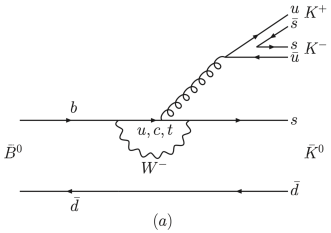
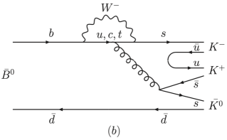
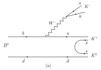
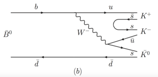
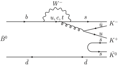
One expects large contributions to the amplitude from i) , the Wilson coefficient being the dominant one (see Table 1 of Ref. PLB699_102 ) and from ii) because these terms are proportional to the kaon form factors. The quark processes involved in these terms can be represented by the Feynman diagrams depicted in Figs. 1 to 3. The wavy lines stand for exchanges, the spring-like lines, if any, for a gluon and the straight lines with an arrow pointing to the right (left) for a quark (antiquark). The short distance contribution of corresponds to the color favored tree diagram shown in Fig. 1(a). The color suppressed term of arises from the tree diagram drawn in Fig. 1(b). The contributions of , and can be represented by the penguin diagrams of Fig. 2 and that of by the penguin diagram of Fig. 3. The factorized forms given in Eqs. (II) can be understood if, in the diagrams of Figs. 1 to 3 one replaces the very heavy meson exchange by a vacuum state creation.
In a way similar to that developed in Ref. DedonderPol for the decays, the detailed expressions for the different amplitudes which build up the contributions can be given as product of short distance terms [sum of ] by long distance ones which can be expressed or are given in terms of meson-meson form factors. As mentioned in the previous paragraph, the amplitudes coming from the terms , and are directly proportional to the kaon form factors. For one has to evaluate the matrix elements of transitions to two-kaon states. As in the previous studies PRD96_113003 , assuming this transition to proceed through the dominant intermediate resonances, it can be approximated, either by a phenomenological function calculated via a unitary equation, or as being proportional to the isovector kaon form factors. In the calculation of the scalar product of two matrix elements in Eqs. (II) one makes use of Eqs. (B1) and (B6) of Ref. ChengPRD76_094006 . As argued above, only the important parts of the amplitude, needed to reasonably reproduce the currently available experimental total branching fraction and the Belle PRD82_073011 and BABAR PRD85_112010 Dalitz plot projections, are given in next Section.
| Parameter | Value | Reference |
|---|---|---|
| 0.1561 | PDG2022 | |
| 0.209 | bene03 | |
| 0.18 | El-Bennich_PRD79 | |
| 0.52 | bene03 | |
| 0.14 | KimPRD67 |
III Dominant contributions to the amplitude
We will give the dominant parts of the decay amplitude and, applying charge conjugation transformation, the corresponding ones. Within this transfomation, the final mesons will be exchanged with the ones and the Mandelstam invariants with the ones. The decay constants and the fixed form-factor values entering our model are given in Table 2. The values for the quark and meson masses are listed in Table 3. For the parts of the amplitude arising from the term [see Eqs. (II)] which involve the calculation of the transition to two kaons, viz. our derivation will follow partly that reported in appendix A of Ref. DedonderPol for the matrix element completed by the use of an equation similar to Eq. (20) of Ref. JPD_PRD103 .
As seen in the previous Section the different contributions to the amplitude are proportional to the sums of the effective Wilson coefficients555As pointed out in the paragraph below Eq. (10) the meson position in the pair matters. (11). We show below that these sums are given by the functions , , , and [see Eqs. (15), (23), (30) and (39)]. Following Ref. PLB699_102 , for the calculation of the Wilson coefficients, we take into account one-loop vertex and penguin corrections but neglect hard scatering ones. Then one has , and . We use the corresponding NLO values calculated and given in Ref. PLB699_102 . These are evaluated at the renormalization scale bene03 .
| 0.0022 | 0.0047 | 0.095 | 4.18 |
|---|---|---|---|
| 0.139570 | 0.497611 | 0.493677 | 5.27963 |
III.1 Contributions to the amplitude with two kaons in wave
III.1.1 The contribution
We retain the part coming from the term in Eqs. (II) where the final forms a scalar and isoscalar state [see Fig. 2(b)]. We have for this term
| (14) |
with [see Eqs. (12), (II) and also Eq. (11) in Ref. PLB699_102 ]
| (15) |
The intermediate scalar-isoscalar resonances for invariant masses 1.6 GeV JPD_PRD103 correspond to the family, mainly , and which we denote as . Using the and quark equations of motion and Eq. (B6) of Ref. ChengPRD76_094006 one gets
| (16) |
For the to transition form factor, we take Ball_PRD71_014015
| (17) |
where and GeV2. One introduces (Eq. (10) of Ref. fkll ) the strange form factor with
| (18) |
The quantity is related to the vacuum quark condensate, as in Ref. fkll we use
| (19) |
where is the charged pion mass. Then we obtain the following contribution for the case,
| (20) |
For the we have
| (21) |
with, from charge conjugation symmetry, and .
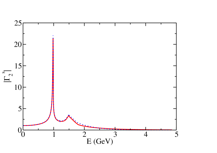
The form factor has been caculated by B. Moussallam Moussallam_2000 ; Moussallam_2020 in the Muskhelishvili-Omnès (MO) dispersion-relation framework Barton1965 ; MO . B. Moussallam has used the updated matrix of the (channel 1), (channel 2) and effective (channel 3) coupled-channel model of Ref. EPJ . Details on this scattering matrix can be found in Appendix A of Ref. JPD_PRD103 . As can be seen in Fig. 4 the modulus of () has a threshold peak which is due to the resonance. The bump near 1.5 GeV arises from the opening of the third effective channel close to where is the mass JPD_PRD103 ; EPJ . Here, the matrix has several poles located nearby and these have an important influence on the energy behavior of in this region. These poles could be related to the and resonances. In our model, we use the form factor corresponding to the red solid line of Fig. 4 where , , equal and , respectively.
III.1.2 The contribution
As seen from Eqs. (12) and (II), the contribution gives rise to the part with the pair in a scalar-isovector state (see Figs. 1(a) and 3). One has,
| (22) |
where the short distance part, similar to Eq. (6) of Ref. PLB699_102 , is
| (23) |
In the evaluation of the long distance matrix element , we assume that the transitions of to the states go first through intermediate meson resonances which then decay into a pair. This decay is described by a vertex function . For the intermediate resonances, as can be seen in Table 1, we have and . Then using Eqs. (B1) and (B6) of Ref. ChengPRD76_094006 Eq. (22) leads to
| (24) | |||||
being the charged kaon decay constant (Table 2). Assuming that the variation of the to transition form factor from one resonance to the other is small, we choose to be which we denote as . We can then parametrize the sum over the resonances by666This parametrization is quite similar to that of Eq. (20) introduced in Ref. JPD_PRD103 for the case.
| (25) |
where we use
| (26) |
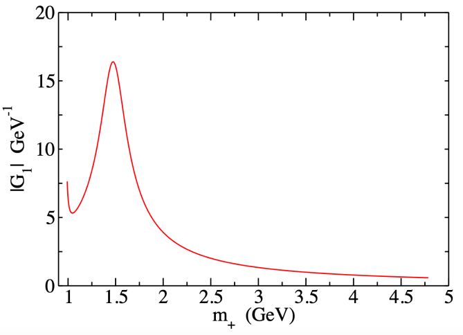
The function describes the transition from a pair into a state. It is calculated from a unitary model with relativistic equations for the two-coupled channels and . It is based on the two-channel model of the and resonances built in Refs. AFLL ; AFLL2 . Details on its calculation are given in chapter IV of Ref. JPD_PRD103 , in particular, see Eqs. (104) to (111). The function depends on two parameters and which represent the coupling constants to the and states, respectively. In our model, is taken as a free parameter with as in Ref. JPD_PRD103 , keeping however the third-degree polynomial fixed to 1. The modulus of the function used in the present model is plotted in Fig. 5. From Eqs. (24) and (III.1.2) we get the following contribution to the amplitude777 An alternative PRD96_113003 could be to parametrize the transition to as being proportional to the scalar-isovector form factor. This form factor has been calculated in Ref. Bachir2015 using MO dispersion relation approach Barton1965 ; MO .
| (27) |
Charge conjugation transformation applied to Eq. (27) gives the following contribution for the case,
| (28) |
where with and .
III.2 Contributions to the amplitude with two kaons in wave
III.2.1 The contributions
Retaining the part coming from [see Figs. 1(b) and 2(a)] one has for this term of the amplitude [Eqs. (12) and (II)],
| (29) |
with (see also Eq. (8) in Ref. PLB699_102 )
| (30) |
and (Eq. (5) in Ref. PLB699_102 )
| (31) |
In the above term only -waves contribute. Following Eq. (B6) in Ref. ChengPRD76_094006 for the evaluation of the matrix element , we obtain
| (32) |
with or . For the vector transition form factor, one can use, as in Ref. PLB699_102 , the parametrization given by Eq. (30) of Ref. Ball_PRD71_014015 ,
| (33) |
with and GeV.
Reference Bruch_2005 provides an evaluation of the form factor using vector dominance, quark model assumptions and isospin symmetry. It receives contributions from the , and resonances as well as those from the , and resonances888 In the following the several and resonances wiil be denoted as and , respectively.. Following Eq. (23) of Ref. PLB699_102 ,
| (34) |
with
| (35) |
and
| (36) |
Here the are the energy-dependent Breit-Wigner functions defined for each resonance of mass and width as
| (37) |
The parameters have been determined in Ref. Bruch_2005 through a constrained fit to the electromagnetic kaon form factors and we use the values given in their Table 2.
The fifth term, [see Fig. 2(b)], in Eqs. (II) yields also only a -wave contribution,
| (38) |
with (see also Eqs.( 10) in Ref PLB699_102 )
| (39) |
The form factor , described in terms of the and resonances denoted as and , is given by (see Ref. Bruch_2005 and also Eq. (25) of Ref.PLB699_102 )
| (40) |
As above for the contributions of the and resonances, the Breit-Wigner functions are given by Eq. (37) and the coefficients by the constrained fit results of Table 2 of Ref. Bruch_2005 .
Adding the contributions of Eqs. (32) and (38) gives for the case,
| (41) | |||||
The corresponding part is
| (42) |
with , , .
III.2.2 The contributions
From the term, using Eq. (B6) of Ref. ChengPRD76_094006 together with relations similar to those of the Eqs. (A.15) to (A.19) of Ref. DedonderPol , one obtains, for the vector-isovector mode, the following contribution to the amplitude (see Figs. 1(a) and 3)
| (43) |
where since it is associated to the , and resonances. The sum over the vertex functions can be parametrized using the vector-isovector form factor PRD96_113003 and,
| (44) | |||||
with the choice and being the charged decay constant (Table 2). From Eqs. (III.2.2) and (44) one gets for the
| (45) | |||||
The Wilson coefficient combination is given by Eq. (23). The value used for the transition form factor, determined in Ref. bene03 , is given in Table 2. As shown in Ref. Bruch_2005 the form factor, gets contributions from the three resonances [see Eq. (36)].
The part reads
| (46) | |||||
with , and .
III.3 Contributions to the amplitude with states in wave
One cannot form a two-kaon -wave state from the vacuum state through the operator, consequently there is no such part arising from the terms for and 6. Here the contribution coming from the term (see Figs. 1(a) and 3) with a two-kaon -wave state, saturated by the resonance, reads (see e.g. Eq. (A.23) of Ref. DedonderPol ),
| (47) | |||||
With one obtains for the case
| (48) |
where the Wilson coefficient combination is given by Eq. (23). The coupling constant characterizes the strength of the transition. The function is defined by
| (49) |
In the center-of-mass system the moduli of the and momenta are given by
| (50) |
and
| (51) |
The transition form factor follows from Ref. KimPRD67 and reads
| (52) |
The form factors, and are not known. In our model we will fix in Eq. (52) to the resonance mass squared and the value we use is given in Table 2. For the case, we have
| (53) |
with , and . The function of the and momenta in center-of-mass system is defined in a similar way to that of the function in Eq. (49) but the variables and have to be interchanged.
IV Results and discussion
The Belle PRD82_073011 and BABAR PRD85_112010 Collaboration analyses of the data have been performed within a time-dependent-Dalitz approach. As shown in Appendix A [see Eq. (80)] the double differential branching fraction or the Dalitz plot density distribution for the decay can be written as
| (54) |
where is our decay amplitude for the process, is that for the decay and is the width. The different parts, and , of our decay amplitudes have been given in Sec. III. The parameter gives the strength of the contribution of the - transition process. It is equal to
| (55) |
where is the difference of the heavy and light mass eigenvalues and is the fraction of events in which the other meson is tagged with the incorrect flavor PRD85_112010 . The double differential branching fraction or the Dalitz plot density distribution for the decay reads
| (56) |
Here, compared to the case, the amplitude arguments and are interchanged.
As in the Belle PRD82_073011 and BABAR PRD85_112010 analyses the sum over both charge-conjugate-decay modes is implied, we compare the experimental effective , and mass projections with the corresponding theoretical distributions obtained by a suitable integration over or of the sum of the differential branching fractions given by Eqs. (54) and (56). Here denote the squares of the three different , and effective masses of the final kaon pairs, respectively.
We have made a simultaneous fit of the model parameters to the Belle data presented in Fig. 3 of Ref. PRD82_073011 and the BABAR data shown in Fig. 17 of Ref. PRD85_112010 . The background components have been subtracted to obtain the signal Belle distributions. We have also omitted the first data bins in the effective mass projections corresponding to the values smaller than their kinematical limits given by the masses of the pairs. Among the Belle data, one has 76 points for the mass distribution, 76 points for the mass distribution, 149 points for the mass distribution and 24 points concentrated in the narrow region of the mass around the resonance. Each set of the three BABAR distributions consists of 32 points. Altogether we have taken into account 325 Belle data points and 96 BABAR data values. As we fit also the branching fraction of the decay, the total number of the data points is equal to 422.
The theoretical values of the , and mass distributions have been related to the branching fraction distributions using the relation
| (57) |
where and
| (58) |
In this expression is the total number of experimental events of a given distribution with the bin width and is the experimental branching fraction of the decay. For the description of the Belle data we use for every while for the BABAR data sets we have , and events.
| Parameters | Values | |
|---|---|---|
| rad | ||
| GeV3/2 | ||
| rad | ||
In our fit we use the function defined as
| (59) |
where
| (60) |
is the experimental value of the mass distribution taken at and is its uncertainty while is the corresponding theoretical value calculated at the same . We put to get a good fit for the theoretical -averaged branching fraction .
It turns out that to obtain a reasonable fit to the data one needs to modify the five components of the model amplitude. The amplitudes and are multiplied by a sixth order polynomial of the variable with
| (61) |
This introduces 8 real free parameters, , and the to 6. The scalar-isovector terms and terms [Eqs. (27) and (28)] are proportional to the function in which the coupling constant [see the paragraph below Eq. (26)] has been adjusted. Both terms have been multiplied by the phase factor , where is a real free parameter. The and - wave components , , , and the -wave and ones need to be renormalized by the free real coefficients , and , respectively.
In our fit, we use the measured ratio PDG2022 and we put the experimental parameter , to get from Eq. (55) the value . The values of the 13 fitted parameters are given in Table 4. We obtain which divided by the number of degrees of freedom, , leads to . The total experimental branching fraction, PDG2022 , is very well reproduced as one gets the corresponding theoretical value equal to .
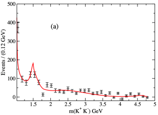
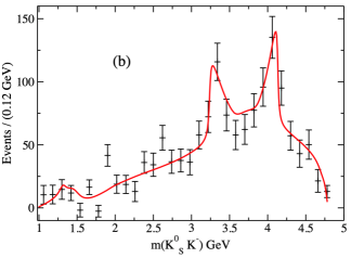
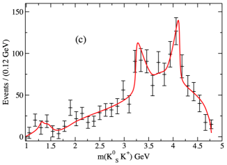
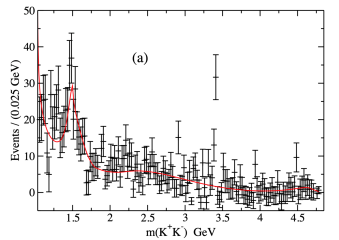
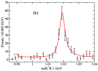
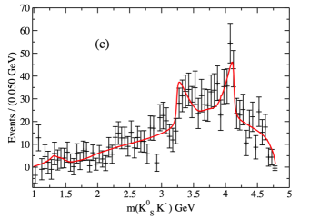
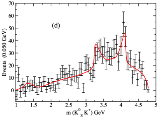
Our fit (solid line) to the mass projection distributions of the Belle PRD82_073011 and BABAR PRD85_112010 experimental data is displayed in Figs. 6 and 7, respectively. The near threshold peak in the distribution of the Belle Collaboration, Fig. 6 (a), is due to the and the next one to the denoted as in Ref. PRD82_073011 . The bump near 1.5 GeV in the plot (Fig. 4) of the modulus of the strange scalar form factor contributes to this peak. Furthermore, in our model, it corresponds to the opening, close to , of the third effective channel JPD_PRD103 ; EPJ . There are also some contributions from the and . The resonance visible at around 3.4 GeV in this Fig. 6 (a) has not been introduced in our amplitude. In Fig. 6 (b) the threshold bump arises from the and the peak is well reproduced. In Figs. 6 (c) and (d) the first bump comes from the and the two other ones are reflections of the . Besides the fact that the projection distribution in the region has not been plotted and that the signal has not been kept, the BABAR distributions, in Fig. 7, have characteristics similar to those of Belle.
For the total branching fraction we obtain which can be compared with . The corresponding sum of these two branching fractions is equal to . Then the total CP asymmetry,
| (62) |
equals %. If one neglects the transitions then this asymmetry becomes %.
The sum of the integrated branching fractions for the and decays into the system are calculated for the particular contributions of the modified and terms. The values and the ratios are given in Table 5 together with their sums for to 5. We see that the term, with an -wave- state, dominates with a contribution of 83.0 % of the total branching fraction. It arises mainly from the mode. The second sizable contribution to , with 18.3 % of the total, is the term with the pair in -wave. It is dominated by plus small and modes. Then follows the mode with 6.2 %, the with 0.15 % and the with 0.11 %. The total percentage sum is 107.7 % which indicates a small interference contribution.
| Final state modes | Contributing | |||
|---|---|---|---|---|
| resonances | ||||
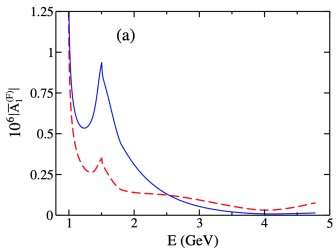
The results shown in Table 5 tell us that the contribution to the amplitude with two kaons in isoscalar wave is very important. It is instructive to plot the modulus of the modified contribution, and to compare it to the modulus of , this is done in Fig. 8(a). The fit to the data requires a reduction of below 2.5 GeV and to an increase above which is done by as seen in Fig. 8 (b). Our strange kaon form factor is too large in the energy range below 2.5 GeV and too small above. Besides this strange form factor the to transition form factor enters the expression of [Eq. (20)] and the product of these two form factors is constrained by the data. The given by Eq. (17) and evaluated in Ref. Ball_PRD71_014015 from light cone sum rules is in good agreement with that recently calculated in a fully relativistic lattice QCD approach PRD_107.014510 . This can be seen comparing the values given by the parametrization (17) to those of the curve of Fig. 16 and Table VI of Ref. PRD_107.014510 .
The Dalitz-plot dependence of CP asymmetry in the framework of a QCDF model for the has been compared to LHCb PRL111_101801 and BABAR PRD85_112010 data in Ref. KKK . In a recent publication PRD108_012008 the LHCb Collaboration has reported measurement of CP asymmetries in charmless three-body decays of . They have shown their distributions as a function of the three-body phase space and have interpreted them as possibly arising from rescattering and resonance interference effects.
For the decays the CP asymmetry in the Dalitz plot can be defined using Eqs. (54) and (56) as follows:
| (63) |
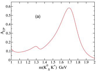
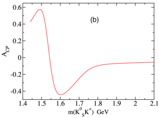
In a large part of the Dalitz plot the values are rather small but there are some regions with GeV where they can be sizable. For instance, in Fig. 9 (a) we show a plot of as a function of for =3.5 GeV. Here we encounter large positive asymmetry values. A small maximum at GeV can be attributed to an influence of the resonance present in the two-kaon-D-wave contribution of the modified term. The second higher maximum has no direct resonant character. It can be related to an interplay of the two-kaon-S-wave contributions of the modified and terms. For other values of and , for example, as seen in Fig. 9 (b), at GeV and for 1.55 GeV GeV a significant negative asymmetry is found while for 1.4 GeV GeV the asymmetry is large and positive. Also for =4 GeV and in the whole range of the kinematically allowed values from 1 GeV to 3.4 GeV the asymmetry is large and positive for below 1.55 GeV and negative above. After integrations on in the Dalitz plot and as noted below Eq. (62), the total CP asymmetry, equal to 0.11%, is small.
The time dependent asymmetry is usually written as
| (64) |
where is defined as the time interval between the decays of the mesons coming from the state, while and are coefficients which can depend on the Dalitz plot variables like and . These coefficients can be calculated as ratios of integrals over some parts of the Dalitz plot, namely999See Eqs. (81) to (86). and , where
| (65) |
| (66) |
and
| (67) |
In Eq. (67) the angle is that of the unitarity triangle PDG2022 . One can see that, when the integration is performed over the full Dalitz plot, the coefficient is equal to the CP asymmetry with a minus sign, .
Using PDG2022 and integrating over and for three specific ranges of , we obtain the and values given in Table 6. One notices a sign flip of the coefficient when going from the range dominated by the meson contribution to the range outside of . The change of the sign is related to the presence of an additional minus sign in the amplitude with respect to the corresponding amplitude. The charge symmetry of the -wave amplitudes is responsible for that effect. The numerical values of the time dependent CP-asymmetry parameters are in qualitative agreement with the experimental results of the BABAR Collaboration presented in Fig. 18 of Ref. PRD85_112010 . The value in the region, 0.53, is compatible with that of BABAR, 0.66 0.17 0.07, given in Table XIII of Ref PRD85_112010 .
V Summary and concluding remarks
In view of further amplitude analyses, in particular by LHCb and Belle II Collaborations, we have derived a decay amplitude in a quasi-two-body QCDF framework. Our derivation follows that developed for the study of CP violation in the decays DedonderPol . The dominant parts of the decay amplitude are calculated in terms of kaon form factors or to two kaons transition functions which describe the final state two-body resonances and their interferences. Unitarity constraints are satisfied when two of the three kaons are in a scalar state. The kaon form factors and transition functions entering this amplitude are similar to those introduced in the Dalitz plot studies of the decays in a factorization approach JPD_PRD103 , the final kaon states being identical. However, here, the larger phase space tests our model over a wider energy range. The kaon-kaon interactions in the , , and waves are taken into account.
Starting from the effective weak decay Hamiltonian Ali1998 ; Beneke:2001ev , a QCDF derivation of the full amplitude within a quasi-two-body framework can be performed. The different terms [see Eqs. (II)] appear as products of short distance contributions, sums which depend on effective Wilson coefficients [see Eq. (11)], times long distance ones given by kaon form factors or parametrized with to transition functions. Some parts of the amplitude, where the formation of the final takes place via an implicit or explicit quark pair, are expected to lead to small contributions. We have neglected these OZI OZI suppressed terms.
The dominant part of the full amplitude has five components and our model reproduces well the Belle PRD82_073011 and BABAR PRD85_112010 Collaborations data. With 13 strong interaction free parameters modifying the five terms of our amplitude, we fit the 422 observables consisting of the total branching fraction together with the Dalitz-plot projections of Belle and BABAR with a of 583.6 which leads to a of 1.43.
The largest contribution to the branching fraction, 83.0 % of the total as seen in Table 5, comes from the modified and terms where the pairs are in a scalar-isoscalar state (see the penguin diagrams of Fig. 2 (b)). These terms are proportional to the strange scalar-isoscalar form factor receiving a large contribution from the , and resonances (see Fig. 4). The dominance of the -resonance contributions was also found in the data analyses of the Belle PRD82_073011 and BABAR PRD85_112010 Collaborations.
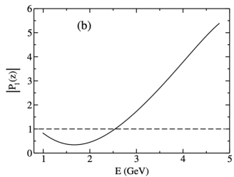
The best fit is obtained if the and terms [Eqs. (20), (21)] are multiplied by the phenomenological complex polynomial with (see Eq. (61), Fig. 8 (b) and Table 4). It leads to a reduction of and below 2.5 GeV and to an increase above [see Fig. 8 (a)]. Within our approach, and for a given to transition form factor , the fit to the Belle PRD82_073011 and BABAR PRD85_112010 data would require for the modulus of our strange kaon form factor , a smaller (larger) value for below (above) 2.5 GeV.
The next important mode, with a branching fraction equal to 18.3% of the total is mainly the one plus some small and arising from the modified and amplitudes. The dominant part with the contribution comes from the term proportional to [Eq. (39)]. The parameters, for the -wave form factors and [Eqs. (34) and (40)] have been determined in Ref. Bruch_2005 using vector dominance, quark model assumptions and isospin symmetry. The best fit requires these and [Eqs. (41) and (42)] contributions to be renormalized by a real parameter which is, however, close to 1 (see Table 4).
The modified terms and with two kaons in a wave of isospin 1, have a branching faction of 6.2 % of the total. Their long distance part depends upon the function whose calculation, given by Eqs. (104) to (111) of Ref. JPD_PRD103 , is based on the - and -channel model of the and resonances built in Refs. AFLL ; AFLL2 . To obtain a good fit, we found necessary to adjust for the function the coupling to the state and to multiply the and terms, [Eqs. (27) and (28)] by the phase factor (see Table 4). The contributions of the resonances were not introduced in the Belle PRD82_073011 and BABAR PRD85_112010 Collaboration analyses.
The remaining amplitudes and (contributions of the , , and resonances and renormalized by the real parameter ), and (-wave saturated by the resonance and multiplied by the real parameter ) give small branching fractions of the order of 0.1%.
For effective masses above 1.7 GeV our model predicts large CP asymmetries in the Dalitz plot, as can be seen in Figs. 9 (a) and (b). We have also calculated the values of the time dependent CP-asymmetry parameters and in the region, the value of the parameter, 0.53, agrees, within errors, with that obtained by BABAR analysis PRD85_112010 .
The charmless three-body decay data provides information on the weak interactions and can also be useful for better knowledge of the kaon-kaon strong interactions. Based on our model one can build a parametrization that can be implemented in experimental Dalitz plot analyses. Dalitz-plot amplitude analysis of several charmless three-body -meson decays can lead to a better understanding on the origin of CP asymmetry.
Acknowledgements
We are deeply indebted to Bachir Moussallam for very profitable correspondence and for the communication of the results of his calculation of scalar form factors. We thank Agnieszka Furman for her participation in the early stage of this work. We also acknowledge helpful discussions with Emi Kou, Mathews Charles and Eli Ben-Haim. This work has been partially supported by a grant from the French- Polish exchange program COPIN/CNRS-IN2P3, collaboration 23-155.
Appendix A - mixing and time-dependent decay rate
The quantum mechanical formalism for neutral particle-antiparticle oscillations and CP violation has been studied and presented in the book of I. I. Bigi and A. I. Sanda CP_Violation2000 (herafter cited as BS). Recent developments on the - mixing can be found in the review by O. Schneider B0_B0barmixing in the 2022 Review of Particle Physics PDG2022 . In this appendix, following BS we show how one can derive Eq. (3) of the BABAR study of CP violation in Dalitz-plot analyses of the charmless hadronic decay PRD85_112010 . We also give the derivation of Eqs. (54), (56) and (64).
A.1 - mixing
The expressions for the time evolution of and states are given by (see Eqs. (6.47) and (6.48) of BS)
| (68) |
with101010 is denoted as and as in Sec. IV.
| (69) |
In Eq. (69) and , i. e. (see Eq. (11.2) of BS). Here and correspond to the masses and widths of the long-life and short-life states, respectively. The time-dependent differential decay rate can be written as
| (70) |
where equal to is the neutral B meson lifetime. Applying the BS master equations (11.15) to (11.22) one obtains for the decay (Eq. (11.58) of BS):
| (71) |
where is the decay amplitude and (see Eq. (6.49) of BS)
| (72) |
being the decay amplitude. For the definition of and see e.g. Eqs. (6.22) to (6.25) of BS. In the case one has (Eq. (11.45) of BS and Ref. PDG2022 ),
| (73) |
where is one of the angles of the CKM triangle. From Eqs. (71) and (72) one gets
| (74) |
Following Eqs. (70) and (74) the time dependent double differential branching fraction of the decay, with and , reads (with the replacement of by )
| (75) | |||||
and that of the
| (76) | |||||
This shows the agreement of Eqs. (75) and 76) with Eq. (3) of Ref. PRD85_112010 for . Integrating over the time from minus to plus infinity and with,
| (77) |
and
| (78) |
one obtains from Eqs. (75) and (76)
| (79) |
and
| (80) |
where (introducing here the dependence) . Eqs. (79) and (80) correspond to Eqs. (56) and (54).
A.2 Time dependent asymmetry
Integrating over and and denoting by the total branching fraction without - mixing, one obtains from Eqs. (75) and (76) for the decay
| (81) | |||||
and for the decay
| (82) | |||||
The time dependent asymmetry defined as
| (83) |
is usually written as
| (84) |
From Eqs. (81), (82) one obtains111111As seen from Eqs. (79) and (80) the - mixing cancels when adding and branching fractions with mixing.
| (85) |
and
| (86) |
References
- (1) Y. Nakahama et al. (Belle Collaboration), Measurement of CP violating asymmetries in decays with a time dependent Dalitz approach, Phys. Rev. D 82, 073011 (2010).
- (2) J. P. Lees et al. (BABAR Collaboration), Study of CP violation in Dalitz-plot analyses of , and , Phys. Rev. D 85, 112010 (2012).
- (3) Thomas Grammatico, Measurement of the branching fractions of decays in LHCb, insights on the CKM angle , and monitoring of the Scintillating Fibre Tracker for the LHCb upgrade, Doctor of Philosophy thesis, Sorbonne Université, January 2022, pdf available on Google.
- (4) Emilie Bertholet, Eli Ben-Haim, Bhubanjyoti Bhattacharya, Matthew Charles, and David London, Extraction of the CKM phase using charmless three-body decays of mesons, Phys. Rev. D 99, 114011 (2019).
- (5) I. Adachi et al. (Belle II Collaboration), Measurement of CP asymmetries in decays with Belle II, Phys. Rev. D 108, 072012 (2023).
- (6) R.L. Workman et al. (Particle Data Group), Review of Particle Physics, Prog. Theor. Exp. Phys. 2022, 083C01 (2022).
- (7) H-Y. Cheng, C-K. Chua and A. Soni, Charmless three-body decays of mesons, Phys. Rev D 76, 094006 (2007).
- (8) A. Garmash et al. (Belle Collaboration), Study of meson decays to three-body charmless hadronic final states, Phys. Rev. D 69, 012001 (2004).
- (9) H.-Y. Cheng, C.-K. Chua, Branching fractions and direct CP-violation in charmless three-body decays of mesons, Phys. Rev. D 88, 114014 (2013).
- (10) The LHCb collaboration, Updated branching fraction measurements of decays, JHEP 11, 027 (2017).
- (11) H.-Y. Cheng, C.-K. Chua and Z.-Q. Zhang, Direct CP-violation in charmless three-body decays of mesons, Phys. Rev. D 94, 094015 (2016).
- (12) Z.T. Zou, Y. Li, Q.X. Li, X. Liu, Resonant contributions to three-body decays in perturbative QCD approach, Eur. Phys. J. C 80, 394 (2020).
- (13) S.-H. Zhou, X.-X. Hai, R.-H. Li and C.-D. Lü, Analysis of three-body charmless -meson decays under the factorization-assisted topological-amplitude approach, Phys. Rev. D 107, 116023 (2023).
- (14) A. Furman, R. Kamiński, L. Leśniak, P. Żenczykowski, Final state interactions in decays, Phys. Lett. B 699, 102 (2011).
- (15) R. Aaij et al. (LHCb Collaboration), Measurement of Violation in the Phase Space of and Decays, Phys. Rev. Lett. 111 (2013) 101801.
- (16) L. Leśniak, P. Żenczykowski, Dalitz-plot dependence of asymmetry in decays, Phys. Lett. B 737, 201 (2014).
- (17) G. Barton, Introduction to Dispersion Techniques in Field Theory (Benjamin, New York, 1965)
- (18) J.-P. Dedonder, R. R Kamiński, L. Leśniak and B. Loiseau, Dalitz plot studies of decays in a factorization approach, Phys. Rev. D 103, 114028 (2021).
- (19) J.-P. Dedonder, A. Furman, R Kamiński, L. Leśniak and B. Loiseau, Final state interactions and CP violation in decays, Acta Phys. Pol. B 42, 2013 (2011) and arXiv:1011.0960v2 [hep-ph].
- (20) Okubo, S., -meson and unitary symmetry model, Phys. Lett., 5, 1975 (1963); Zweig, G., An SU(3) model for strong interaction symmetry and its breaking. Version 2, CERN Report No. 8419 TH 412, 1964 (unpublished); Iizuka, J., A systematics and phenomenology of meson family, Prog. Theor. Phys. Suppl. 37, 38 (1966).
- (21) D. Boito, J.-P. Dedonder, B. El-Bennich, R. Escribano, R. Kamiński, L. Leśniak, and B. Loiseau, Parametrization of three-body hadronic - and -decay amplitudes in terms of analytic and unitary meson-meson form factors, Phys. Rev. D 96, 113003 (2017).
- (22) A. Ali, G. Kramer and Cai-Dian Lü, Experimental tests of factorization in charmless nonleptonic two-body decays, Phys. Rev. D 58, 094009 (1998).
- (23) M. Beneke, G. Buchalla, M. Neubert and C. T. Sachrajda, QCD factorization in decays and extraction of Wolfenstein parameters, Nucl. Phys. B606, 245 (2001).
- (24) M. Tanabashi et al. (Particle Data Group), Review of Particle Physics, Phys. Rev. D 98, 030001 (2018).
- (25) M. Beneke and M. Neubert, QCD factorization for and decays, Nucl. Phys. B675, 333 (2003).
- (26) B. El-Bennich, O. Leitner, J.-P. Dedonder, B. Loiseau, Scalar meson in heavy-meson decays, Phys. Rev. D 79, 076004 (2009).
- (27) C. S. Kim, J.-P. Lee and S. Oh, Nonleptonic two-body charmless B decays involving a tensor meson in the ISGW2 model, Phys. Rev. D 67, 014002 (2003).
- (28) P. Ball and R. Zwicky, New results on decay form factors from light-cone sum rules, Phys. Rev. D 71, 014015 (2005).
- (29) A. Furman, R. Kamiński, L. Leśniak and B. Loiseau, Long-distance effects and final state interactions in and decays, Phys. Lett. B 622, 207 (2005).
- (30) B. Moussallam, dependence of the quark condensate from a chiral sum rule, Eur. Phys. J. C 14, 111 (2000).
- (31) B. Moussallam, private communication, May 2020.
- (32) N. I. Muskhelishvili, Singular integral equations, chapters 18 and 19, (P. Nordhof 1953); R. Omnès, On the solution of certain singular integral equations of quantum field theory, Nuovo Cim. 8, 316 (1958).
- (33) R. Kamiński, L. Leśniak and B. Loiseau, Scalar mesons and multichannel amplitudes, Eur. Phys. J. C 9, 141 (1999).
- (34) A. Furman, L. Leśniak, Coupled channel study of resonances, Phys. Lett. B 538, 266 (2002).
- (35) A. Furman, L. Leśniak, Properties of the resonances, Nucl. Phys. B (Proc. Suppl.) 121, 127 (2003).
- (36) M. Albaladejo and B. Moussallam, Form factors of the isoscalar scalar current and the phase shifts, Eur. Phys. J. C 75, 488 (2015).
- (37) C. Bruch, A. Khodjamirian, J. H. Kühn, Modeling the kaon form factors in the timelike region, Eur. Phys. J. C 39, 41 (2005).
- (38) W. G. Parrott, C. Bouchard, and C. T. H.Davies (HPQCD Collaboration), and form factors from fully relativistic lattice QCD, Phys. Rev. D 107 014510 (2023).
- (39) R. Aaij et al. (LHCb Collaboration), Direct CP violation in charmless three-body decays of mesons, Phys. Rev. D 108, 012008 (2023).
- (40) I. I. Bigi and A. I. Sanda, CP Violation, Cambridge University Press 2000.
- (41) O. Schneider (EPFL), - mixing, https://pdg.lbl.gov rpp2022-rev-b-bar-mixing.