Thermal analysis of black hole in de Rham–Gabadadze–Tolley massive gravity in Barrow entropy framework

Abstract

This study examines a recently hypothesized black hole solution in de Rham–Gabadadze–Tolley massive gravity. Firstly, we consider the negative cosmological constant as a thermodynamic pressure. We extract the thermodynamical properties such as Hawking temperature, heat capacity and Gibbs free energy using the Barrow entropy. We also obtain a new pressure associated to the perfect fluid dark matter and discuss the first-order van der Waals-like phase transition. This black hole’s stability is investigated through specific heat and Gibbs free energy. Also, we analyze the thermodynamic curvatures behavior of black hole through geometry methods (Weinhold, Ruppeiner, Hendi-Panahiyah-Eslam-Momennia (HPEM), and geometrothermodynamics (GTD)).
Keywords: Black hole in dRGT massive gravity; Thermodynamic Quantities; Thermal Geometries.

I Introduction and Motivation

One of the most exciting and stimulating area of study is the geometrical structure of black hole (BH) in general theory of relativity (GR) [1]. Exciting phenomena in de Rham–Gabadadze–Tolley (dRGT) massive gravity testing the recognition of D-bound and Bekenstein bound provides the phantom background and excluding quintessence fields with cosmological constant. In Ref.[2], there is discussion of entropy bounds testing the plausibility of the cosmological constant includes other areas or more details, refer to [3].

Additionally, the Bekenstein limit displays the highest entropy limit on the physical system (Universe-BH system). This change (D bond) does not provide the guarantee of physical behavior, so no additional energy can be introduced into the Bekenstein bond. It is worth to mentioning here that there are many efforts to proposing extensions of Einstein’s general theory of relativity to explain the current accelerating expansion of the Universe. In GR, the curvature singularity is an identification of breakdown; this is broadly revealed to the existence and its requisite in quantum gravity because it is a more primitive theory of gravitation [4]. For the first time, Hawking investigated the BH temperature, in this case he observed that BH can emit radiations near the event horizon from side-to-side gravitational interactions. Also, Hawking and Page constructed the stable phase transition between the Schwarzschild BH and the pure radiation (gas) [5, 6]. The quantum scenario concerning Hawking radiation, this gives us a precious clue that a BH has its temperature directly connected to its area gravity and that its entropy is proportional to the horizon area. These results have shown that there exist a deep association between thermodynamics and gravity [7]. Later on, the phase transition and liquid-gas phase transition were investigated for charged and rotating AdS BHs; in this case, there exists a small or large BHs and van der Waals fluid [8, 9, 10]. On other hand, in extended phase space thermodynamics studies where we put the key association between the cosmological constant (thermodynamic pressure) and its conjugate variable (thermodynamic volume) [11]. Most impressive characteristics studied for AdS BHs thermodynamics through quantum gravity space-time to have BH horizon, which provides an accumulation of concepts from the GR and the thermodynamics in quantum field theory[12].

Afterward, the thermodynamic characteristics of BHs have been widely studied, such as thermodynamical behavior for BHs through Riemannian geometry [13, 14, 15]. This Ruppeiner’s metric by taking the thermodynamic potentials corresponding to the mass by Legendre transformations [16, 17]. The construction of thermodynamic geometry in the context of nonlinear electrodynamics, this provides the interpretation of the microstructure for various BHs. It is testing to generalize the thermodynamic curvature to understand the microstructure of BHs; in this scenario, it is indelible complications relating to the first law of BH and Lagrangian formations are integrated with nonlinear electrodynamics rather than linear ones. In particular, to study the direct relation between the phase transitions and curvature singularities of Weinhold’s [18] and Ruppeiner’s [19, 20] interpretations, which are manifested through a Hessian matrix in terms of entropy and internal energy respectively. Recently, numerous approaches have been made to inaugurate the different geometries phenomenon into the ordinary thermodynamics [13, 14, 18, 19, 20]. Hermann [21] investigated the effects of the thermal geometries phase space system as a differential manifold (natural contact structure), which provides a particular subspace of equilibrium states in the thermodynamics. A new metric Hendi-Panahiyah-Eslam-Momennia (HPEM metric) was introduced in order to build a geometrical phase space by thermodynamical quantities which shows that the characteristics behavioral of Ricci scalar $R^{HPEM}$ of this metric enables one to recognize the type of phase transition and critical behavior of the BHs near phase transition points. Also, the geometrothermodynamics (GTD) of this BH and investigated the adaptability of the curvature scalar of geothermodynamic methods with phase transition points of the BH. Also, in GTD of this black hole and investigated the adaptability of the curvature scalar of geothermodynamic methods with phase transition points of BH. The geometrical interpretation is a great deal for exploring the microstructure of BHs thermodynamic system [16, 17, 21, 22, 23, 24, 25, 26, 27, 28, 29, 30, 31]. According to one thought, interactions in the system under the study of microscopic statistical features have been illustrated through thermodynamic amounts induced from these geometries [24, 25, 26, 27, 28, 29, 30, 31, 32]. Even though the geometrothermodynamics (GTD) methods for various BHs are studied, it remains unexplored in case of BH in dRGT massive gravity via Barrow entropy. This provides us a good opportunity to bridge the gap.

In this paper, we use thermodynamic Barrow entropy and study thermodynamic quantities as well as thermodynamic geometric methods for BH in massive gravity dRGT. To evaluate the Barrow entropy of the BH in the massive gravity dRGT due to thermal fluctuations, we exploit the expressions for the Hawking temperature and specific heat. Additionally, using standard thermodynamic relationships, we calculate mass and the heat capacity. For the mass in terms of Barrow entropy reaches a maximum value at $S_{B}=4.0$ $(=S_{Bm})$, after that it becomes zero at point $S_{B}=9.5$ with the fixed values $\alpha$, $\beta$ , $c$ and $m_{g}$. In case of heat capacity, we find that, the heat capacity remains negative in the range of $0<S_{B}<1$ (unstable phase). However, with values of $S_{B}\leq 1$, this leads to stable phase transition. We study the behavior of Gibbs free energy $G$, which represents an equilibrium state at constant pressure. The Gibbs free energy $G$ is a fundamental quantity and provides information about the first-order phase transition of BH in the massive gravity dRGT. Furthermore, we analyze the thermodynamic geometry of such BH. To do this, we plot the thermodynamic quantities and scalar curvature of the Weinhold, Ruppeiner and GTD methods against Barrow entropy. We find that the singular curvature points are scalars of the Weinhold and GTD methods with Barrow entropy. These geometrical methods, along with others, provide invaluable information about the nature of BH, their formation, evolution and related phenomena. In this way, they form the basis of BH physics and contribute significantly to our understanding of the most mysterious objects in the universe.

In section II, we discuss the fundamental details of BH solution in dRGT massive gravity. Within section, we study the various thermodynamics of the solution together with the thermal stability of BH in dRGT massive gravity in the presence of Barrow entropy. In section III, we investigate the thermal geometries of BH with Barrow entropy. Finally, in section IV, we provide the discussions and final remarks.

II Brief Review of BH solution in dRGT massive gravity

Einstein’s gravity escorts a massive gravity associated with a scalar field. Therefore, we added a suitable nonlinear term in the Einstein-Hilbert action as follows [33]

$$S=1/(16\pi)\int d^{4}x\sqrt{-g}\left[\Re+m_{g}^{2}\bigsqcup\left(g,\phi^{a}\right)\right],$$ (1)

where $\bigsqcup$ is a potential, and $\Re$ is the Ricci scalar for the graviton, which changes the action with the graviton parameter $m_{g}$ which represents the graviton mass. The action is expressed in terms of units so that $G=1$. In four-dimensional spacetime, the effective potential $\mathcal{U}$ is expressed as follows

$$\bigsqcup\left(g,\phi^{2}\right)=\bigsqcup_{2}+\alpha_{3}\bigsqcup_{3}+\alpha_{4}\bigsqcup_{4},$$ (2)

where constants $\alpha_{3}$ and $\alpha_{4}$ represent the dimensionless free parameters of the theory and the symmetric potentials along with reliance on metric $g$ and scalar field $\phi^{a}$. The term $\kappa^{n}$ typically represents a parameter or a coupling constant raised to the power of $n$. The parameter $\kappa$ commonly appears in gravitational theories and often represents the gravitational coupling constant. Its precise value depends on the choice of units and the particular gravitational theory being considered. These can be written as

$$\begin{gathered}\bigsqcup_{2}\equiv[\kappa]^{2}-\left[\kappa^{2}\right],\\ \bigsqcup_{3}\equiv[\kappa^{3}-3[\kappa]\left[\kappa^{2}\right]+2\left[\kappa^{3}\right],\\ \bigsqcup_{4}\equiv[\kappa]^{4}-6[\kappa]^{2}\left[\kappa^{2}\right]+8[\kappa]\left[\kappa^{3}\right]+3\left[\kappa^{2}\right]^{2}-6\left[\kappa^{4}\right],\end{gathered}$$ (6)

where $[\kappa]$ is eigenvalues of matrix $\delta^{\mu}_{\nu}-\sqrt{g^{\mu\eta}f_{\xi\sigma}\partial_{\eta}\phi^{\xi}\partial_{\nu}\phi^{\sigma}}$. Where, $f_{\xi\sigma}$ is a reference metric and $[\mathcal{K}]=\mathcal{K}_{\mu}^{\mu}$ is a trace. One can split the gauge condition by selecting the unitary gauge and imposing an additional restriction on the Stückelberg scalars. The scalar field $\phi^{a}$ has an upper index, leading to a convention that can be used to distinguish these fields from other types of variables in the theory. In this case, the use of capital letters for scalar fields can be treated as emphasize to their meaning or conform to symbols commonly used in related fields of the theoretical physics. This is simply a matter of convention for clarity and consistency in the specific context of dRGT massive gravity. We choose a unitary gauge $\phi^{a}=x^{\mu}\delta_{\mu}^{a}\mid$, in this measurement, five graviton degrees are described by the metric $g_{\mu\nu}$. Stückelberg scalar transformation equals to the coordinate transformation. According to this selection, it is possible to break the state of measure and make the additional modifications in the Stückelberg scalar. $\phi^{a}$ is introduced as a scalar field to recover the general covariance so-called Stückelberg scalar theory. The term $\kappa^{n}$ typically represents a parameter or a coupling constant raised to the power of $n$. The parameter $\kappa$ commonly appears in gravitational theories and often represents the gravitational coupling constant. Its precise value depends on the choice of units and the particular gravitational theory being considered. For simplicity, one can rewrite the free parameters (constants) $\alpha_{3}$ and $\alpha_{4}$ in terms of new parameters $\alpha$ and $\beta$ as $\alpha_{3}=\frac{\alpha-1}{3}$ and $\alpha_{4}=\frac{\beta}{4}+\frac{1-\alpha}{12}$. The static and spherically symmetric BH solutions of the modified Einstein equations can be written as a line element:

$$ds^{2}=-f(r)dt^{2}+\frac{dr^{2}}{f(r)}+h(r)^{2}d\Omega^{2},$$ (7)

This can be categorized and arrange into $d(r)=0$( $h(r)=h_{0}r$) here $h_{0}$ is a constant in the form of $\alpha$ and $\beta$ respectively [34, 35, 36, 37]. One can consider $h(r)=r$ in the line element to have a BH solution. So, a particular class of results of dRGT massive gravity with the symmetries. Therefore, we are interested in these symmetries because this is a good deal in the degree of freedom of the solutions and has an important consequences to discuss the stability. The metric function $f(r)$ follows as

$$f(r)=1-\frac{2M}{r}+\frac{\Lambda}{3}r^{2}+\gamma r+\zeta,$$ (8)

where

$$\begin{gathered}\Lambda=3m_{g}^{2}(1+\alpha+\beta),\\ \gamma=-cm_{g}^{2}(1+2\alpha+3\beta),\\ \zeta=c^{2}m_{g}^{2}(\alpha+3\beta).\end{gathered}$$ (12)

Here, $M$ represents the integration constant that associated with the BH mass, and $c$ is a constant used in the reference metric. Here the cosmological constant $\Lambda$ depends (linked) to the graviton mass $m_{g}$. So, the graviton mass $m_{g}$ has a connotation for the accelerated Universe expansion. One would be interested in whether the BH solutions in this theory can converge to the Schwarzschild solution in general relativity under certain conditions. Research in this area typically includes to studying the equations of motion and solutions extracting from the dRGT theory and analyzing whether they reduce to the well-known Schwarzschild solution in general relativity with appropriate limits, such as when the graviton mass $m_{g}$ and free parameters $(\alpha,\beta)$ become zero $m_{g},\alpha,\beta=0$.

II.1 Barrow Entropy

In Ref. [38], Barrow studied the prospects that quantum-gravitational forces could provide an impenetrable, modifying the BH real horizon region and fractal structure on the BH surface. According to Barrow, the effects of quantum gravity change the standard entropy relation $S=\frac{A}{4}$ to $S=A^{1+\frac{\Delta}{2}}$, where $A$ is the actual surface and $\Delta$ represents the quantum gravitational distortion effect. Keeping in mind the importance of Barrow entropy, we study the impact of BH thermodynamics in dRGT theory. We analyze the physical engine of the Barrow formula. The Bekenstein-Hawking entropy plays a fundamental role in the three-dimensional model of dark energy, where $S_{BH}=A/(4G)$ and it is used at the [39, 40] horizon. Although Barrow BH entropy was built as a toy model, some theoretical evidence supports its idea. As a result, a new BH entropy relation follows as

$$S_{B}=\bigg{(}\frac{A}{A_{0}}\bigg{)}^{1+\frac{\Delta}{2}}.$$ (13)

Here, $A_{0}$ represents the Planck area; at this stage, $A$ is the ordinary horizon area. Besides, it is linked with Tsallis entropy (nonextensive) expression [41]; this entropy is different from the quantum corrected entropy [42] with logarithmic. It provides the most straightforward construction for distinctive values such as $\Delta=0$. One can obtain the well-known result as Bekenstein-Hawking entropy with $\Delta=0$; we have the maximal deformation in this case.

II.2 Thermal Stability

In thermal analysis, it is well-known that a cosmological constant can be considered as a thermodynamic pressure and the thermodynamic pressure $P$ of the BH can be incorporated into the first law of thermodynamics. Belonging to the horizon condition $f(r)|_{r=r_{h}}=0$ along with Barrow entropy and the pressure relation is $P=-\frac{\Lambda}{8\pi}=\frac{3}{8\pi l^{2}}$ [4, 6, 8], one can extract the expression connecting to the BH mass as follows

$$M = \frac{1}{6}(\pi^{-\frac{\Delta}{2}-1}{S_{B}})^{\frac{1}{\Delta+2}}\left[3c^{2}m_{g}^{2}(\alpha+3\beta)-3cm_{g}^{2}(2\alpha+3\beta+1)(\pi^{-\frac{\Delta}{2}-1}{S_{B}})^{\frac{1}{\Delta+2}}\right.$$ (14)

$$- \left.8\pi P(\pi^{-\frac{\Delta}{2}-1}{S_{B}})^{\frac{2}{\Delta+2}}+3\right].$$

In Figs. 2 and 2, we show the effect of BH mass with the Barrow entropy. We see that in Fig. 2, the mass of BH reaches a maximum value at $S_{B}=4.0$ $(=S_{Bm})$, after that it becomes zero at point $S_{B}=9.5$ with the fixed values $\Delta$ and $\alpha$, respectively.

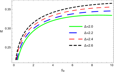
Figure 1: Plot of mass vs the Barrow entropy with fixed parameters as $\alpha=0.30$, $\beta=0.20$, $c=2.50$ and $m_{g}=0.25$.

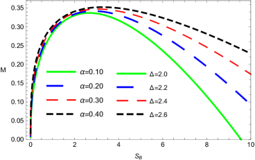
Figure 2: Plot of mass vs the Barrow entropy with fixed parameters as $\beta=0.20$, $c=2.50$ and $m_{g}=0.25$.

The physical and non-physical characteristics of BH can be discussed by analyzing the Hawking temperature. The positive value of temperature ensures the physical solution while the non-physical solution is given by its negative value. After recognizing the thermodynamic behavior of BH, it is worth to exploring the phase transition points and the divergency points of heat capacity. With the well-known relation $T=\frac{f^{\prime}(r_{h})}{4\pi}$, temperature of BH can be calculated as

$$T = \frac{(\pi^{-\frac{\Delta}{2}-1}{S_{B}})}{4\pi}^{-\frac{1}{\Delta+2}}\left[c^{2}m_{g}^{2}(\alpha+3\beta)-2cm_{g}^{2}(2\alpha+3\beta+1)(\pi^{-\frac{\Delta}{2}-1}S_{B})^{\frac{1}{\Delta+2}}\right.$$ (15)

$$- \left.8\pi P(\pi^{-\frac{\Delta}{2}-1}S_{B})^{\frac{2}{\Delta+2}}+1\right].$$

The first law of BH thermodynamics can be expressed as [4, 6, 8, 9, 10]

$$dM=TdS+VdP+\Phi d\alpha+\Psi d\beta+\aleph dm_{g}+C_{1}dc,$$ (16)

where $M$, $P$, $V$, $S$, and $\Phi$ are the mass, pressure, volume, entropy, and chemical potential, respectively. Here, the $\Psi$, $\aleph$ and $C_{1}$ are the conjugate variables. The thermodynamic parameters symbolize to the conjugating variables $\beta$, $m_{g}$ and $c$, respectively. The volume $V$ and chemical potential $\Phi$ of BH are defined as

$$V=\bigg{(}\frac{\partial M}{\partial P}\bigg{)}_{S,q},\ \ \ \ \ \Phi=\bigg{(}\frac{\partial M}{\partial\alpha}\bigg{)}_{S,P}.$$ (17)

The Barrow entropy, with the help of first law thermodynamics, follows as

$$V = \frac{1}{3}(-4)\pi\left(\pi^{-\frac{\Delta}{2}-1}S_{B}\right)^{\frac{3}{\Delta+2}},$$ (18)

$$\Phi = -\frac{1}{2}cm_{g}^{2}\left(\pi^{-\frac{\Delta}{2}-1}S_{B}\right)^{\frac{1}{\Delta+2}}\left(2\left(\pi^{-\frac{\Delta}{2}-1}S_{B}\right)^{\frac{1}{\Delta+2}}-c\right),$$ (19)

$$\Psi = \frac{1}{2}(-3)cm_{g}^{2}\left(\pi^{-\frac{\Delta}{2}-1}S_{B}\right)^{\frac{1}{\Delta+2}}\left(\left(\pi^{-\frac{\Delta}{2}-1}S_{B}\right)^{\frac{1}{\Delta+2}}-c\right),$$ (20)

$$\aleph = cm_{g}\left(\pi^{-\frac{\Delta}{2}-1}S_{B}\right)^{\frac{1}{\Delta+2}}\left(c(\alpha+3\beta)-(2\alpha+3\beta+1)\left(\pi^{-\frac{\Delta}{2}-1}S_{B}\right)^{\frac{1}{\Delta+2}}\right),$$ (21)

$$C_{1} = -\frac{1}{2}m_{g}^{2}\left(\pi^{-\frac{\Delta}{2}-1}S_{B}\right)^{\frac{1}{\Delta+2}}\left((2\alpha+3\beta+1)\left(\pi^{-\frac{\Delta}{2}-1}S_{B}\right)^{\frac{1}{\Delta+2}}-2c(\alpha+3\beta)\right).$$ (22)

The pressure can be expressed as

$$P=\frac{-6\alpha cm_{g}^{2}V^{\frac{2}{3}}-9\beta cm_{g}^{2}V^{\frac{2}{3}}-3cm_{g}^{2}V^{2/3}+4\sqrt[3]{6}\pi^{\frac{2}{3}}M-12\pi TV^{\frac{2}{3}}}{8\sqrt[3]{6}\pi^{\frac{2}{3}}V}.$$ (23)

The effect of Barrow entropy is seen in the progression plots in Figs. 4-6, where the pressure consistently proscribes the original behaviour of all the isotherms and squeezes them to the critical isotherm. The green curve represents the behavior greater than critical point $T>T_{c}$. Also, it appears that the Barrow entropy parameter removes the fluctuating isotherms at the upper limit of its strength. This may be presented as the maximum temperature value $T$ that exterminates the van der Waals-like nature of the BH in dRGT massive gravity.

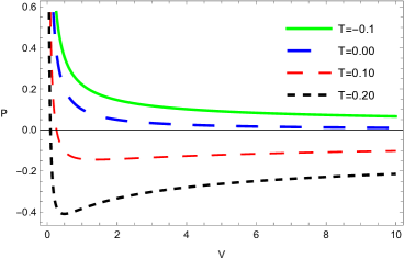
Figure 3: Plot of pressure $P$ vs. $V$ with fixed parameters such as $M=0.3$, $\alpha=0.5$, $\beta=0.02$, $c=1$ and $m_{g}=0.02$.

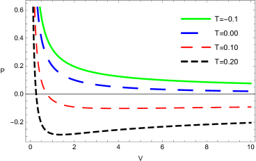
Figure 4: Plot of pressure $P$ vs. $V$ with fixed parameters such as $M=0.6$, $\alpha=0.5$, $\beta=0.02$, $c=1$ and $m_{g}=0.02$.

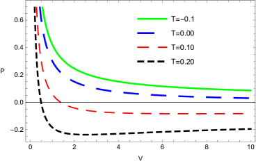
Figure 5: Plot of pressure $P$ vs. $V$ with fixed parameters such as $\alpha=0.5$, $M=0.9$, $\beta=0.02$, $c=1$ and $m_{g}=0.02$.

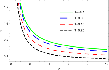
Figure 6: Plot of pressure $P$ vs. $V$ with fixed parameters such as $\alpha=0.5$, $M=1.2$, $\beta=0.02$, $c=1$ and $m_{g}=0.02$.

With the help of the standard definition of heat capacity [4, 15]

$$C=\bigg{(}\frac{\partial S}{\partial T}\bigg{)}_{P}T,$$ (24)

one can be calculated as

$$C=\frac{2\pi(\Delta+2)S_{B}(\pi^{-\frac{\Delta}{2}-1}S_{B})^{\frac{3}{\Delta+2}-1}\ (\pi^{-\frac{\Delta}{2}-1}S_{B})^{\frac{\Delta}{\Delta+2}}}{-c^{2}m_{g}^{2}(\alpha+3\beta)+cm_{g}^{2}(2\alpha+3\beta+1)(\pi^{-\frac{\Delta}{2}-1}S_{B})^{\frac{1}{\Delta+2}}-1}.$$ (25)

To evaluate the Barrow entropy of the BH in the massive gravity dRGT due to thermal fluctuations, we exploit the expressions for the Hawking temperature and specific heat. Additionally, using the standard thermodynamic relationships, we plotted the graph of heat capacity which provides the first-order phase transition. In case of heat capacity, we obtain that, the heat capacity remains negative in the range of $0<S_{B}<1$ (unstable phase). However, with values of $S_{B}\leq 1$, this leads to stable phase transition in Figs. 8 and 8. We study the behavior of the Gibbs free energy $G$, which represents equilibrium at constant pressure. The Gibbs free energy $G$ is a fundamental quantity and provides information about the first-order phase transition of BH in the massive gravity dRGT. However, with the specified values of $S_{B}\leq 1$, one can observe an unstable to stable region, and the stable phase transition (see after the values of $S_{B}=1$). Finally, in the presence of Barrow entropy, we present an unstable to a stable phase transition with fixed values $M=1.2$, $\alpha=0.5$, $\beta=0.02$, $c=1$ and $m_{g}=0.02$.

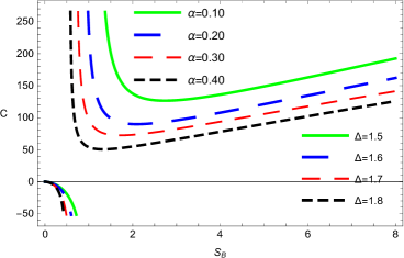
Figure 7: Plot of $C$ with fixed parameters as $\beta=0.20$, $c=0.44$ and $m_{g}=1.80$.

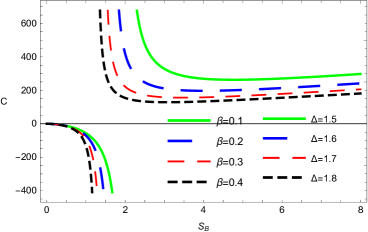
Figure 8: Plot of $C$ with fixed parameters as $\alpha=0.20$, $c=0.44$ and $m_{g}=1.80$.

The Gibbs free energy can be estimated from the well-known definition as

$$G=M-TS_{B}.$$ (26)

This leads to

$$G=2^{\frac{1}{3}(-2)(\Delta+6)}3^{\frac{\Delta}{3}}\pi^{\frac{\Delta-4}{6}}V^{\frac{\Delta}{3}}\left(6^{\frac{2}{3}}cm_{g}^{2}V^{\frac{2}{3}}(2\alpha+3\beta+1)-8\pi^{\frac{2}{3}}M-16\pi^{\frac{2}{3}}PV\right)+M.$$ (27)

Let us discuss here the Euclidean method also to calculate the Gibbs free energy. In the Euclidean action $\mathcal{S}_{E}$ is expressed by the analytic continuation of the action $S=iS_{E}$ [43, 44, 45, 46], this is associated to the partition function

$$Z=e^{-\mathcal{S}_{E}},$$ (28)

where time is defined as $\tau=it$. According to statistical mechanics, the relationship between free energy and partition function is

$$G=-T\ln\mathcal{Z}=T\mathcal{S}_{E}.$$ (29)

In addition, to calculate the expression of temperature, we apply a fixed temperature boundary condition throughout Euclidean time as [43, 45]

$$\int d\tau=\frac{1}{T\sqrt{f\left(r_{B}\right)}}.$$ (30)

On the other hand, the time period $\tau$ is given by the inverse of the Hawking temperature $1/T_{h}$, this can written as

$$T=\frac{T_{h}}{\sqrt{f\left(r_{B}\right)}}.$$ (31)

The concrete expression for the temperature of a static and BH solution in de Rham–Gabadadze–Tolley massive gravity follows as

$$T=\frac{-\frac{3r_{h}^{2}}{l^{2}}+\xi+2\gamma r_{h}+1}{4\pi\sqrt{f(r_{B})}r_{h}},$$ (32)

where

$$f(r_{B})=\frac{\frac{r_{h}^{3}-r_{B}^{3}}{l^{2}}+(r_{B}-r_{h})(\xi+\gamma r_{B}+\gamma r_{h}+1)}{r_{B}}.$$ (33)

For the static symmetrically metric, we evaluate the Euclidean action related to the metric function as

$$\begin{aligned} \mathcal{S}_{E}=&-\frac{1}{T\sqrt{f\left(r_{B}\right)}}\int_{r_{h}}^{r_{B}}\left(-2f^{\prime}(r)-rf^{\prime\prime}(r)+\frac{2r}{l^{2}}\right)dr\\ &-\frac{2}{T\sqrt{f\left(r_{B}\right)}}\left(f\left(r_{B}\right)+\frac{r_{B}^{2}}{l^{2}}-\frac{r_{B}\sqrt{f\left(r_{B}\right)}}{l}\right),\\ \end{aligned}$$ (34)

calculated as

$$\begin{aligned} \mathcal{S}_{E}=-\frac{2\left(f(r_{B})l^{2}-\sqrt{f(r_{B})}lr_{B}-\gamma l^{2}r_{B}+r_{h}\left(\gamma l^{2}-2r_{h}\right)+3r_{B}^{2}\right)}{\sqrt{f(r_{B})}l^{2}T}.\end{aligned}$$ (35)

Thus, from Eqs.(29) and (35), the free energy is expressed as

$$G=\frac{2\left(-f(r_{B})l^{2}+\sqrt{f(r_{B})}lr_{B}+\gamma l^{2}r_{B}+r_{h}\left(2r_{h}-\gamma l^{2}\right)-3r_{B}^{2}\right)}{\sqrt{f(r_{B})}l^{2}}.$$ (36)

In Figs. 10 and 10, we can observe a minimum behavior of $G$, which represents an equilibrium state at constant pressure. In this scenario, a $G$ in dRGT massive gravity is a fundamental quantity providing phase transitions either small or large BHs. So, we have observed the first-order phase transition. In addition, Gibbs free energy is a analysis to provide overall stability of a BH.

Figure 9: Plot of Gibbs free energy $G$ with fixed parameters as $\alpha=0.10$, $\beta=0.50$, $c=1.50$, $\Delta=1.40$ and $m_{g}=1.80$.

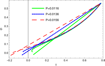
Figure 10: Plot of Gibbs free energy $G$ with fixed parameters as $\alpha=0.10$, $\beta=0.50$, $c=1.50$, $\Delta=1.40$ and $m_{g}=1.80$.

It is well known that thermodynamics of a black hole include three famous mass formulas, i.e., the first law of thermodynamics, the Bekenstein-Smarr mass formula, and the Christodoulou-Ruffini squared-mass formula. Here, we have only considered the first law of thermodynamics. However, it can also be tested through the the Bekenstein-Smarr relation and the Christodoulou-Ruffini-type squared-mass formula [47, 48, 49, 50, 51].

III Thermal Geometries

We study the geometrical structures of the BH surrounded by quintessence field by calculating the Weinhold, Ruppiner, GTD and HPEM curvature scalars. However, we observed that the positive (stable) BH behaviour for specific range such as $S_{B}\leq 0.78$. Also, these trajectories provide the attractiveness along with the repulsive behaviour of BH. Also for the HPEM formalism, there is another divergency of HPEM metric which coincides with the singular points of heat capacity and therefore we can extract more information rather than other mentioned metrics [18, 19, 20, 16, 17, 21, 22, 23, 24]. The scalar curvature can be associated with the relationship between divergence at the critical point and volume of the system. Generally, the line element for the BH is given by

$$ds^{2}=\frac{SM_{S}}{\left(\prod_{i=2}^{n}\frac{\partial^{2}M}{\partial\xi_{i}^{2}}\right)^{3}}\left[\Sigma_{i=2}^{n}\left(\frac{\partial^{2}M}{\partial\xi_{i}^{2}}\right)d\xi_{i}^{2}-M_{SS}dS^{2}\right].$$ (37)

where $\xi_{i}\neq S$ and $M_{S}$ denotes the derivative of mass $M$ with respect to the entropy $S$. The intrinsic expression of the metric space follows as

$$g=\left(E^{c}\frac{\partial\phi}{\partial E^{c}}\right)\left(\eta_{ab}\delta^{bc}\frac{\partial^{2}\phi}{\partial E^{c}\partial E^{d}}dE^{a}dE^{d}\right),$$ (38)

where $\frac{\partial\phi}{\partial E^{c}}=\delta_{bc}I^{b}$, $\phi$, $I^{b},E^{a}$ and in turn, notions the extensive, thermodynamic potential, and intensive thermodynamic parameters respectively. This section is studies for thermodynamic geometries such as Weinhold, Ruppeiner, HPEM and GTD formalisms. Despite numerous works on BH thermodynamics, a details discussion regarding the microstructure of BH was still missing. Illustration of Weinhold geometry formulated as

$$g_{ij}^{W}=\partial_{i}\partial_{j}M(S_{B},l).$$ (39)

The Weinhold metric follows as

$$ds^{2}_{W}=M_{S_{B}S_{B}}dS_{B}^{2}+M_{ll}dl^{2}+2M_{S_{B}l}dS_{B}dl,$$ (40)

with the following matrix form:

$$\begin{pmatrix}M_{S_{B}S_{B}}&M_{S_{B}l}\\ M_{lS_{B}}&M_{ll}\\ \end{pmatrix}.$$ (41)

One can obtain the the curvature scalar $(R^{W})$ using the above equations, calculated as

$$R^{W} = \left[(\Delta-2)l^{2}S_{B}^{\frac{3}{\Delta+2}}(S_{B}^{\frac{3}{\Delta+2}}(\pi^{7/2}(\beta+\frac{1}{3})cl^{2}m_{g}^{2}S_{B}^{\frac{2}{\Delta+2}}(\Delta(S_{B}-\frac{3}{2})+2S_{B}-\frac{3}{2})-\frac{3}{2}\pi^{3}(\Delta-2)S_{B}^{\frac{3}{\Delta+2}})\right.$$ (42)

$$+ \left.\left.S_{B}^{\frac{1-\Delta}{\Delta+2}+1}(\pi^{7/2}(\beta+\frac{1}{3})c(\Delta-2)l^{2}m_{g}^{2}S_{B}^{\frac{2}{\Delta+2}}+\pi^{3}(\Delta+2)S_{B}^{\frac{3}{\Delta+2}}))\right]\right/\left[12\pi^{3/2}S_{B}(S_{B}^{\frac{2(1-\Delta)}{\Delta+2}+1}\right.$$

$$- \left.\frac{1}{2}(\Delta-2)S_{B}^{\frac{3}{\Delta+2}}(\sqrt{\pi}(\beta+\frac{1}{3})cl^{2}m_{g}^{2}S_{B}^{\frac{2}{\Delta+2}}+S_{B}^{\frac{3}{\Delta+2}}))^{2}\right].$$

In this case, we demonstrate the positive and negative behavior of $(R^{W})$. We also discuss the curvature behavior and compare it with the heat capacity shown in Figs. 11 and 12. However, we observed that the positive behavior before the singular point such as $S_{B}\leq 0.78$, and the negative after the singular point respectively. Moreover, these trajectories provide the attractiveness along with the repulsive behavior of BH in de Rham–Gabadadze–Tolley massive gravity. This provides the phenomenological information about either repulsive or attractive characteristics between its molecules. Also, these trajectories provide the attractiveness along with the repulsive behaviour of BH. We investigated that this BH provides phenomenologically information about either repulsive or attractive characteristics between its molecules.

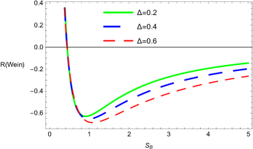
Figure 11: Plot of Weinhold curvature scalar $R^{W}$ with fixed parameters as $\alpha=0.10$, $\beta=1.0$, $c=0.20$, $l=1.50$ and $m_{g}=1.10$.

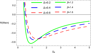
Figure 12: Plot of Weinhold curvature scalar $R^{W}$ with fixed parameters as $\alpha=0.10$, $c=0.20$, $l=1.50$ and $m_{g}=1.10$.

The Ruppeiner geometry conformal (corresponding) to the Weinhold geometry, scalar curvature $R^{Rup}$ is determined as

$$ds^{2}_{R}=\frac{ds^{2}_{W}}{T}.$$ (43)

The explicit expression of Ruppeiner geometry is derived as

$$R^{Rup} = \left[\pi^{\frac{5}{2}}(\Delta-2)l^{2}S_{B}^{\frac{8}{\Delta+2}-1}(\sqrt{\pi}(3\beta+1)cl^{2}m_{g}^{2}(-\Delta+2(\Delta+2)S_{B}-7)-3(\Delta-10)S_{B}^{\frac{1}{\Delta+2}})\right]\times$$ (44)

$$\left[18(S_{B}^{\frac{4-\Delta}{\Delta+2}}-\frac{1}{6}(\Delta-2)S_{B}^{\frac{5}{\Delta+2}}(\sqrt{\pi}(3\beta+1)cl^{2}m_{g}^{2}+3S_{B}^{\frac{1}{\Delta+2}}))^{2}(-(3\beta+1)cm_{g}^{2}-\frac{2(S_{B})}{\sqrt{\pi}l^{2}}^{\frac{1}{\Delta+2}}\right.$$

$$+ \left.(\pi^{-\frac{\Delta}{2}-1}S_{B})^{-\frac{2}{\Delta+2}}(m_{g}^{2}(\alpha+\beta+1)(\pi^{-\frac{\Delta}{2}-1}S_{B})^{\frac{3}{\Delta+2}}+(\pi^{-\frac{\Delta}{2}-1}S_{B})^{\frac{1}{\Delta+2}}))\right]^{-1}.$$

In this case, the negative values gives imaginary roots. So, we start from zero points are $S_{B}=0$ and $S_{B}=S_{Bm}$, respectively. Also it matches with zero point of the temperature as well as the heat capacity, this represents the phase transition point. The curvature scalar $R^{Rup}$ of BH concerning to the horizon’s radius $S_{B}$ is studied in Figs. 14 and 14. In the scenario, the singular points concur with the zero points of heat capacity.

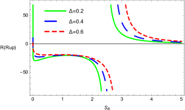
Figure 13: Plot of Ruppeiner curvature scalar $R^{Rup}$ with fixed parameters as $\alpha=0.10$, $\beta=1.80$, $c=0.20$, $l=1.50$ and $m_{g}=0.07$.

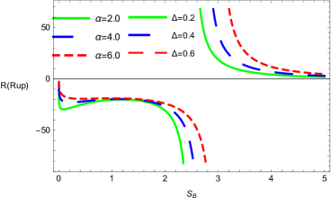
Figure 14: Plot of Ruppeiner curvature scalar $R^{Rup}$ with fixed parameters as $\beta=1.80$, $c=0.20$, $l=1.50$ and $m_{g}=0.07$.

Hence, we observed the thermodynamic phase transition for curvature scalar of the Ruppiner metric in terms of $S_{B}$. A new metric HPEM was introduced in order to build a geometrical phase space by thermodynamical quantities. We show that the characteristics behavioral of Ricci scalar $R^{HPEM}$ of this metric enables one to recognize the type of phase transition and critical behavior of the BHs near phase transition points. This provides us an opportunity to bridge this gap. As a consequence the curvature can be interpreted as a measure of thermodynamic interaction. This is the motivation of present study. The HPEM geometry follows as

$$ds^{2}=\frac{S_{B}M_{S_{B}}}{\left(\frac{\partial^{2}M}{\partial l^{2}}\right)^{3}}(-M_{S_{B}S_{B}}dS_{B}^{2}+M_{ll}dl^{2}).$$ (45)

The mathematically expression for the HPEM geometry scalar is calculated as

$$R^{(HPEM)} = \bigg{[}l^{8}S_{B}^{-\frac{6}{\Delta+2}-1}(3\sqrt{\pi}\beta cl^{2}m_{g}^{2}S_{B}^{\frac{2}{\Delta+2}}+\sqrt{\pi}cl^{2}m_{g}^{2}S_{B}^{\frac{2}{\Delta+2}}+3S_{B}^{\frac{3}{\Delta+2}})\times$$ (46)

$$(\pi^{7/2}(\beta+\frac{1}{3})cl^{2}m_{g}^{2}S^{\frac{2}{\Delta+2}}(\Delta(S_{B}-\frac{3}{2})+2S_{B}-\frac{3}{2})-\frac{3}{2}\pi^{3}(\Delta+2)S_{B}^{\frac{3}{\Delta+2}})\bigg{]}$$

$$\times\bigg{[}108(\Delta+2)^{2}(\sqrt{\pi}(\beta+\frac{1}{3})cl^{2}m_{g}^{2}S_{B}^{\frac{2}{\Delta+2}}+S_{B}^{\frac{3}{\Delta+2}})^{2}\bigg{]}^{-1}.$$

From the Figs. 16 and 16, one can see the divergency of scalar curvature of the HPEM metric at zero point; it is close to the heat capacity plot with fixed parameters $\beta=1.80$, $c=0.20$, $l=1.50$ and $m_{g}=0.07$, respectively. Therefore, we extract some beneficial information from the HPEM formalism.

Figure 15: Plot of HPEM curvature scalar $R^{(HPEM)}$ with fixed parameters as $\alpha=2$, $\beta=1.80$, $c=0.20$, $l=1.50$ and $m_{g}=0.07$.

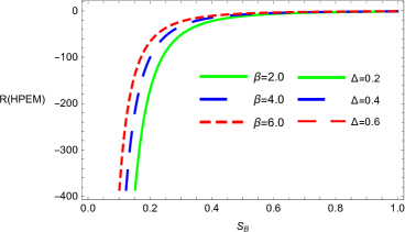
Figure 16: Plot of HPEM curvature scalar $R^{(HPEM)}$ with fixed parameters as $\alpha=2$, $c=0.20$, $l=1.50$ and $m_{g}=0.07$.

The scalar curvature for GTD metric can be formulated as

$$ds^{2}=(-S_{B}M_{S_{B}S_{B}}+lM_{ll})\begin{pmatrix}M_{S_{B}S_{B}}&0\\ 0&m_{ll}\\ \end{pmatrix}.$$ (47)

From the above expression, one can obtain as

$$R^{(GTD)} = \bigg{(}\pi^{3/2}S_{B}^{-\frac{\Delta+4}{\Delta+2}}(\pi^{-\frac{\Delta}{2}-1}S_{B})^{\frac{2}{\Delta+2}}((3\beta+1)cl^{2}m_{g}^{2}+(2\Delta+7)(\pi^{-\frac{\Delta}{2}-1}S_{B})^{\frac{1}{\Delta+2}})$$ (48)

$$(9(\Delta+2)S_{B}^{\frac{1}{\Delta+2}}-\sqrt{\pi}(3\beta+1)cl^{2}m_{g}^{2}(2(\Delta+2)S_{B}-3(\Delta+1)))\bigg{)}$$

$$\times\bigg{[}2(\Delta+2)^{2}(\sqrt{\pi}(3\beta+1)cl^{2}m_{g}^{2}+3S_{B}^{\frac{1}{\Delta+2}})^{2}\bigg{]}^{-1}.$$

We study the GTD curvature scalar behaviour in Figs. 18 and 18. This can be seen that the singular point at $S_{B}=1.21$ for curvature scalar of GTD. Whenever, we plotted the heat capacity in Figs. 8 and 8 with fixed values of $\beta=0.20$, $c=0.44$ and $m_{g}=1.80$ respectively. We observed in that case, the heat capacity was zero at $S_{B}=1$. On can see that, if the singular point $S_{B}=1$ of GTD curvature is not coincident (meet) with the heat capacity. In this scenario, we cannot get any physical information concerning to this frame work from the GTD geometry.

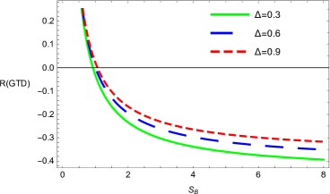
Figure 17: Plot of GTD curvature scalar $R^{W}$ with fixed parameters as $\alpha=2$, $\beta=1.80$, $c=0.20$, $l=2.50$ and $m_{g}=0.07$.

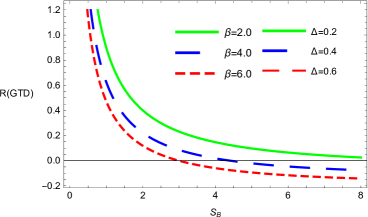
Figure 18: Plot of GTD curvature scalar $R^{W}$ with fixed parameters as $\alpha=2$, $c=0.20$, $l=2.50$ and $m_{g}=0.07$.

IV Concluding Remarks

In this paper, we discussed the thermodynamic behaviour of BH in dRGT massive gravity and investigated the BH thermal geometries. We graphed thermodynamic properties in terms of $S_{B}$, and we presented that where it is minimum or maximum values of the mass, we plotted the mass parameter in Figs. 2 and 2. The cosmological constant is associated to the state parameter pressure $P$, we studied the phase behaviour in Figs. 4-6. In this case, we observed that, if we increase the Barrow entropy parameter, the horizon radius expands and decreases with critical temperature and pressure . On other hand, two divergences points could be seen in Figs. 8-10. Further, we studied the first order phase transition (swallow-tail shape) graphed in $G-T$. We examined the effect of stability behaviour of heat capacity in dRGT massive gravity using the Barrow entropy. We investigated the first order phase transition in the presence of Barrow entropy, this yields leads to an unstable/stable regions. Recently, the similar results have been discussed through thermal quantities of specific BHs in Ref. [52, 53, 54, 55].

In Figs. 12-14, we have observed that the Weinhold and Ruppeiner scalars and matched with singularity points as in heat capacity plots. We found that thermodynamic curvatures such as HPEM and GTD have exhibited the attractive as well as repulsive nature of BH for particular parameters. We have investigated the HPEM and GTD geometries of BH in dRGT massive gravity by fixing phase space of entropy, and pressure as shown in Figs. 16-18. We also distinguished the behaviour between the specific heat and thermodynamic geometries providing the beneficial information of such BH. It would be interesting and stimulating to examine the prospects of similar results also work in most general theories [25, 31, 32, 56, 57].

Finally, the thermal geometries of BH in de Rham–Gabadadze–Tolley massive gravity by using Weinhold, HPEM, Ruppeiner and GTD formalism were presented. We observed the zero of scalar curvature coincided at $S_{B}=0.799$ of BH in de Rham–Gabadadze–Tolley massive gravity. Furthermore, important information about the microstructure of BH is provided by Ruppeiner, HPEM and GTD geometries in the form of divergence of scalar curvature, and similar behavior has been observed at zeros of heat capacity in Ref. [58]. Scalar curvature thus provides important information about the nature of the microscopic interactions described above. These geometric structures thus provide important insight into the critical phenomena and phase structure or divergence of BH in De Rham–Gabadadze-Tolley massive gravity.

Declaration of competing interest

The authors declare that they have no known competing financial interests or personal relationships that could have appeared to influence the work reported in this paper.

Data Availability Statement

This manuscript has no associated data, or the data will not be deposited. There is no observational data related to this article. The necessary calculations and graphic discussion can be made available on request.

References

- [1] R. Ruffini and J.A. Wheeler. Phys. today. 30, 24 (1971).
- [2] H. Hadi, F. Darabi, K. Atazadeh and Y. Heydarzade, Eur. Phys. J. C 80, 12 (2020).
- [3] H. Hadi, F. Darabi and Y. Heydarzade, EPL 131, 5 (2020).
- [4] J.M. Maldacena, Adv. Theor. Math. Phys. 2, 231 (1998).
- [5] S.W. Hawking and D.N. Page, Commun. Math. Phys. 87, 577 (1983).
- [6] S.W. Hawking and D.N. Page, Comm. Math. Phys. 87, 577 (1983).
- [7] E.M.C. Abreu and J.A. Neto, Phys. Lett. B 810, 135805 (2020).
- [8] A. Chamblin, R. Emparan, C.V. Johnson and R.C. Myers, Phys. Rev. D 60, 064018 (1999).
- [9] D. Kubiznak and R.B. Mann, JHEP 1207, 033 (2012).
- [10] D. Kastor, S. Ray and J. Traschen, Class. Quant. Gravit. 26, 195011 (2009).
- [11] B.P. Dolan, Class. Quant. Gravit. 28, 125020 (2011).
- [12] N.D. Birrell and P.C.W. Davies, Cambridge University Press, Cambridge, (1982).
- [13] J. Aman and N. Pidokrajt, Phys. Rev. D 73, 024017 (2006).
- [14] F. Weinhold, J. Chem. Phys. 63, 2479 (1975).
- [15] G. Ruppeiner, Rev. Modern Phys. 67, 605 (1995).
- [16] T. Sarkar, G. Sengupta and B.N. Tiwari, J. High Energy Phys 611, 015 (2006).
- [17] R. Hermann, Phys. and Sys. (Marcel Dekker, New York, 1973).
- [18] G. Ruppeiner, Phys. Rev. A 20, 1608 (1979).
- [19] G. Ruppeiner, Rev. Mod. Phys. 67, 605 (1995).
- [20] J. Aman, I. Bengtsson and N. Pidokrajt, Gen. Relativ. Gravit. 35, 1733 (2003).
- [21] F. Weinhold, J. Chem. Phys. 63, 2479 (1975).
- [22] S.W. Wei, Y.X. Liu and R.B. Mann, Phys. Rev. Lett. 123, 071103 (2019).
- [23] A.G. Tzikas, Phys. Lett. B 788, 219 (2019).
- [24] S. Upadhyay, S. Soroushfar and R. Saffari, Mod. Phys. Lett. A 36, 2150212 (2021).
- [25] C.L.A. Rizwan, A.N. Kumara, K. Hegde and D. Vaid, Ann. Phys. 422, 168320 (2020).
- [26] A.N. Kumara et al. (2021).
- [27] F. Weinhold, Eur. Phys. J. C 77, 110 (2017).
- [28] F. Capela and G. Nardini, Phys. Rev. D 86, 024030 (2012).
- [29] S. Saheb and S. Upadhyay, Phys. Lett. B 804, 135360 (2020).
- [30] S. Soroushfar, R. Saffari and S. Upadhyay, Gen. Rel. Grav. 51, 130 (2019).
- [31] S.H. Hendi, et al., Phys. Rev. D 92, 06402 (2015).
- [32] B.E. Panah, Phys. Lett. B 787, 45 (2018).
- [33] H. Hadi, A.R. Akbarieh and P.S. Ilkhchi, Eur. Phys. J. Plus 138, 330 (2023).
- [34] K. Koyama, G. Niz and G. Tasinato, Phys. Rev. D 84, 064033 (2011).
- [35] K. Koyama, G. Niz and G. Tasinato, Phys. Rev. Lett. 107, 131101 (2011).
- [36] F. Sbisa, G. Niz, K. Koyama and G. Tasinato, Phys. Rev. D 86, 024033 (2012).
- [37] S. G. Ghosh, L. Tannukij and P. Wongjun, Eur. Phys. J. C 76, 119 (2016).
- [38] J. D. Barrow, arXiv:2004.09444.
- [39] R.M. Wald, Phys. Rev. D 48, 3427 (1993).
- [40] E.M. Abreu and J.A. Neto, Eur. Phys. J. C 80, 776 (2020).
- [41] C. Tsallis, J. Stat. Phys. 52, 479 (1988).
- [42] E.N. Saridakis: arXiv:2005.04115.
- [43] Y. Huang and J. Tao, Nucl. Phys. B 982, 115881 (2022).
- [44] J.W. York, Phys. Rev. D 33, 2092 (1986).
- [45] G.W. Gibbons and S.W. Hawking, Phys. Rev. D 15, 2752 (1977).
- [46] P. Wang, H. Wu and H. Yang, J. High Energy Phys. 07, 002 (2019).
- [47] D. Christodoulou, Phys. Rev. Lett. 25, 1596 (1970).
- [48] D. Christodoulou and R. Ruffini, Phys. Rev. D 4, 3552 (1971).
- [49] M. M. Caldarelli, G. Cognola, and D. Klemm, Classical Quantum Gravity 17, 399 (2000).
- [50] S.-Q. Wu and D. Wu, Phys. Rev. D 100, 101501(R) (2019).
- [51] D.Wu, P.Wu, H. Yu, and S.-Q.Wu, Phys. Rev. D 102, 044007 (2020).
- [52] M. Chabab et al., [arXiv:1804.10042].
- [53] J.X. Mo et al., [arXiv:1804.02650].
- [54] M.S. Ali and S.G. Ghosh, Phys. Rev. D 98, 084025 (2018).
- [55] D. Kubiznak and R.B. Mann, JHEP 1207, 033 (2012).
- [56] M. Yasir, K. Bamba and A. Jawad, Int. J. of Mod. Phys. D 30, 2150068 (2021).
- [57] C. Shahid, A. Jawad and M. Yasir, Phys. Rev. D 105, 024032 (2022).
- [58] M.U. Shahzad, M.I. Asjad and S. Nafees, et al., Eur. Phys. J. C 82, 1044 (2022).