Adaptive Whole-body Robotic Tool-use Learning on Low-rigidity Plastic-made Humanoids Using Vision and Tactile Sensors

Abstract

Various robots have been developed so far; however, we face challenges in modeling the low-rigidity bodies of some robots. In particular, the deflection of the body changes during tool-use due to object grasping, resulting in significant shifts in the tool-tip position and the body’s center of gravity. Moreover, this deflection varies depending on the weight and length of the tool, making these models exceptionally complex. However, there is currently no control or learning method that takes all of these effects into account. In this study, we propose a method for constructing a neural network that describes the mutual relationship among joint angle, visual information, and tactile information from the feet. We aim to train this network using the actual robot data and utilize it for tool-tip control. Additionally, we employ Parametric Bias to capture changes in this mutual relationship caused by variations in the weight and length of tools, enabling us to understand the characteristics of the grasped tool from the current sensor information. We apply this approach to the whole-body tool-use on KXR, a low-rigidity plastic-made humanoid robot, to validate its effectiveness.

I INTRODUCTION

Various types of robots have been developed over the years. While there are robots with high rigidity and strong force capabilities, commonly found in industrial applications [1, 2], there exist low-rigidity robots constructed with rubber or plastic-made links and joints [3, 4]. The development of these robots can be driven by different factors, such as the pursuit of flexibility in soft robotics [5], cost considerations, or the need for lightweight design. While high-rigidity robots are easier to model and can execute precise movements, low-rigidity robots pose challenges in modeling due to the flexibility of their joints and links, which can deform in response to posture and external forces. Particularly, although it is possible to apply standard kinematics and dynamics when only the joints have low rigidity, when both joints and links exhibit low rigidity, modeling becomes exceedingly difficult and the application of conventional methods becomes problematic. Methods considering the flexibility of these joints and links have been developed [6, 7], but they still face numerous challenges including the necessity for multiple assumptions and computational complexities when dealing with multi-link systems. In tool-use on low-rigidity robots, the deflection of the body changes due to object grasping, leading to significant variations in the tool-tip position and center of gravity. Furthermore, the amount of the deflection can vary based on the weight and length of tools, further complicating their modeling. In the context of soft robotics, various methods have been developed to learn kinematics and dynamics from flexible and diverse sensors [8, 9, 10]. However, there is currently no method capable of handling changes in the body due to variations in tool grasping.

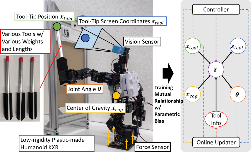
Figure 1: The concept of this study: learning the mutual relationship among joint angle, center of gravity, tool-tip position, and tool-tip screen coordinates for adaptive whole-body tool-use of low-rigidity robots considering the changes in tool weight and length.

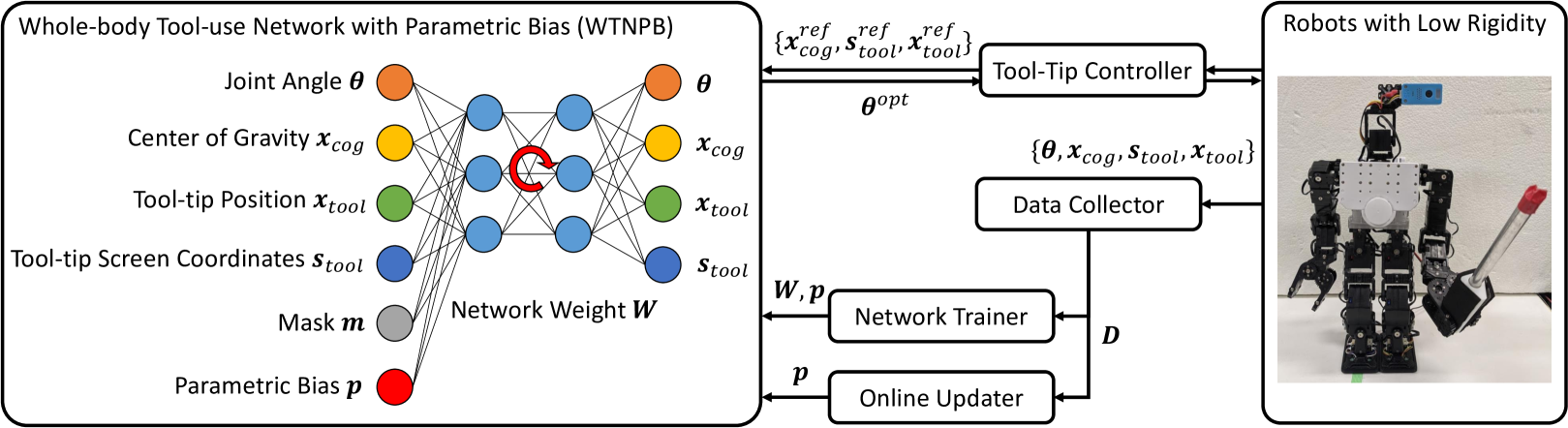
Figure 2: System overview of Whole-body Tool-use Network with Parametric Bias (WTNPB) including Data Collector, Network Trainer, Online Updater, and Tool-Tip Controller for Low-Rigidity Robots.

In this study, we develop a method for controlling tool-tip position considering deflection, using a neural network that describes the mutual relationship among joint angle, visual information, and tactile information for tool-use on low-rigidity robots (Fig. 1). Additionally, since this deflection varies depending on the weight and length of the grasped tool, we estimate this variation from current sensor information using the mechanism of Parametric Bias (PB) [11] to achieve more accurate control. PB is a mechanism that can implicitly embed multiple attractor dynamics within a neural network, and in this study, we utilize it to embed changes in the mutual relationship among sensors. Previous studies on learning-based tool-use have explored various methods for tool selection [12], motion planning [13], and tool understanding [14], but all of them have been conducted with rigid-bodied robots, and few have considered the center of gravity. In the context of imitation learning, methods considering flexible joints exist [15], but flexible links have not been taken into account. Furthermore, since imitation learning requires human demonstrations, its purpose differs from our study, which aims to enable robots to learn the mutual relationship among sensors on their own body. Other approaches using reinforcement learning [16] or self-supervised learning [17] exist, but none of them have considered the flexibility of joints and links, as well as the resulting changes in the body’s center of gravity. While gradual changes in tool grasping states have been considered in some methods [18], our study is novel in that it incorporates tactile information and different visual information, considering the weight and length of tools and the resulting body deflection.

The structure of this study is as follows. In Section II, we discuss the proposed Whole-body Tool-use Network with Parametric Bias (WTNPB) and the overall system, covering the network structure, network training, online update, and control using this network. In Section III, we present experimental results using both a simulation and the actual robot, focusing on network training, state estimation based on online update, and tool-tip position control. Additionally, we perform an integrated tool-use experiment with the low-rigidity humanoid KXR to open a window. In Section IV, we reflect on the experimental results and outline future prospects. In Section V, we provide our concluding remarks.

II Whole-body Robotic Tool-use Learning for Low-Rigidity Robots

The overall system, including the Whole-body Tool-use Network with Parametric Bias (WTNPB) proposed in this study, is illustrated in Fig. 2.

II-A Network Structure

Consider a robot holding a tool in its hand. In this scenario, the network structure of WTNPB can be expressed as follows,

$$\bm{x}^{T} =\begin{pmatrix}\bm{\theta}^{T}&\bm{x}^{T}_{cog}&\bm{x}^{T}_{tool}&\bm{s}^{T}_{tool}\end{pmatrix}$$ (1)

$$\bm{z} =\bm{h}_{enc}(\bm{x},\bm{m},\bm{p})$$ (2)

$$\bm{x} =\bm{h}_{dec}(\bm{z})$$ (3)

$$\bm{h}(\bm{x},\bm{m},\bm{p}) =\bm{h}_{dec}(\bm{h}_{enc}(\bm{x},\bm{m},\bm{p}))$$ (4)

where $\bm{\theta}$ is the commanded joint angle of the robot, $\bm{x}_{cog}$ is the center of gravity position of the robot, $\bm{x}_{tool}$ is the tool-tip position in 3D space, $\bm{s}_{tool}$ is the tool-tip screen coordinates on the camera image, $\bm{m}$ is the mask variable (will be explained later), $\bm{p}$ is Parametric Bias (PB) [11], and $\bm{z}$ is the latent variable. Furthermore, $\bm{h}_{enc}$ is the encoder network, $\bm{h}_{dec}$ is the decoder network, and $\bm{h}$ is the entire network combining these encoder and decoder networks.

As detailed in Section III-A, we use a low-rigidity plastic-made humanoid robot, KXR [4], for our experiments. We define $\bm{\theta}$ as $\begin{pmatrix}\theta_{s-p}&\theta_{s-y}&\theta_{e-p}&\theta_{a-p}\end{pmatrix}^{T}$, representing the commanded joint angle, which include shoulder pitch and yaw angles (s-p, s-y), elbow pitch angle (e-p), and ankle pitch angle (a-p) of KXR. we limit the dimensionality of $\bm{\theta}$ to simplify data collection. The center of gravity position, $\bm{x}_{cog}=\begin{pmatrix}x_{cog}&y_{cog}\end{pmatrix}^{T}$, is calculated from 1-axis tactile sensors placed at the corners of each foot (assuming that the feet remain aligned during tool-use, and disregarding the $z$-direction). $\bm{x}_{tool}$ represents the 3D position of the tool tip recognized using AR markers. $\bm{s}_{tool}$ represents the 2D position of the tool tip recognized using AR markers or color extraction. The variable $\bm{m}$ is used to capture the relationship among multiple modalities contained in $\bm{x}$. Since $\bm{x}$ contains four modalities, $\bm{m}$ is a 4-dimensional vector, where a value of 1 indicates the use of each modality, while 0 indicates its non-use. For example, when $\bm{m}^{T}=\begin{pmatrix}1&1&0&0\end{pmatrix}$, the input $\bm{x}^{T}$ consists of $\begin{pmatrix}\bm{\theta}^{T}&\bm{x}^{T}_{cog}&\bm{0}^{T}&\bm{0}^{T}\end{pmatrix}$, meaning that all $\bm{x}$ are reconstructed from a subset of $\bm{x}$ through $\bm{z}$, forming a network structure. The choice of $\bm{m}$ is not arbitrary, and it requires defining a feasible set $\mathcal{M}$. In this study, as $\bm{\theta}$ serves as both sensor data and commanded values, masks related to $\bm{\theta}$ with a value of $1$ in $\bm{m}$ are all feasible. Additionally, we assume that $\bm{\theta}$ can be inferred from all other modalities. Therefore, we define $\mathcal{M}$ as $\{(1\;0\;0\;0),(1\;1\;0\;0),(1\;0\;1\;0),(1\;0\;0\;1),(1\;1\;1\;0),(1\;1\;0\;1),\\ (1\;0\;1\;1),(0\;1\;1\;1)\}$. This enables the system to adapt to the absence of certain modalities during online update and control. Finally, $\bm{p}$ represents PB that captures changes in the mutual relationship among sensors due to changes in the length and weight of the tool. In this study, we consider it as a 2D vector. Increasing the dimensionality of $\bm{p}$ makes it challenging to structure the space of PB and prone to overfitting, but it allows capturing various changes in the mutual relationship.

In this study, the overall network structure consists of 7 layers. Regarding the number of units, the input is 17-dimensional, composed of 11 dimensions from $\bm{x}$, 4 dimensions from $\bm{m}$, and 2 dimensions from $\bm{p}$. The intermediate layers have the following sizes: $\{200,50,8,50,200\}$, and the output is 11-dimensional corresponding to $\bm{x}$. The middle layer with 8 units represents the dimension of the latent variable $\bm{z}$. We employ the hyperbolic tangent activation function and the Adam optimizer [19] for update. During training, the network input and output are normalized using all collected data.

II-B Training of WTNPB

First, we collect data for various tool states (weight and length), denoted as $k$ ($1\leq k\leq K$, where $K$ is the total number of tool states used for training), in different poses, represented as $D_{k}=\{\bm{x}_{1},\cdots,\bm{x}_{N_{k}}\}$, where $N_{k}$ is the number of data points for tool state $k$. Additionally, we prepare Parametric Bias $\bm{p}_{k}$ as a learnable input variable for each tool state $k$ (all $\bm{p}_{k}$ are initialized to 0). It is important to note that there is no need to explicitly know the specific weight or length of the tools, as the space of PB self-organizes implicitly. We generate the dataset $D_{train}=\{(D_{1},\bm{p}_{1}),\cdots,(D_{N_{k}},\bm{p}_{N_{k}})\}$ and train $\bm{h}$ using this dataset. During training, $\bm{p}_{k}$ is common for data $D_{k}$ but varies across different tool states. The training process involves updating the network weight $W$ and $\bm{p}_{k}$ ($1\leq k\leq K$) simultaneously using backpropagation. Furthermore, we randomly select $\bm{m}$ from $\mathcal{M}$ as a network input. This mechanism allows information about tool state $k$ to be embedded in each $\bm{p}_{k}$, while the space of $\bm{p}$ self-organizes based on the tool state.

The training process consists of two stages. First, we vary the tool state in a simulation to collect data and calculate $W$ and $\bm{p}_{k}$. In this stage, we generate data by randomly moving $\bm{\theta}$ within a specified joint angle range. $\bm{s}_{tool}$ and $\bm{x}_{cog}$ are computed using camera models and kinematic models. For low-rigidity robots, we make a simple model for joint error based on joint torque to obtain data, which assumes an angular deflection of 3.0$\tau$ ($\tau$ is joint torque [Nm]). Subsequently, we retain only the computed $W$ from the simulation and initialize $\bm{p}_{k}$ to $\bm{0}$. Second, we collect data using the actual robot and perform fine-tuning. To facilitate data collection, AR markers are attached to the tool tip, allowing us to collect all values of $\bm{x}$, including $\bm{x}_{tool}$ and $\bm{s}_{tool}$. We employ two methods for data collection. One involves direct human teaching of $\bm{\theta}$ via a GUI, with data collected for each specified pose. The other method randomly decides $\bm{\theta}$ in a simulation, while ensuring that the center of gravity remains within the support area and the tool-tip position is visible from the camera. By imposing strong constraints on the center of gravity position, we can collect data safely within the range of stability, even if there are differences between a simulation and the actual robot. Since the actual robot data is limited, fine-tuning is performed using data from a simulation to adapt to real-world conditions.

II-C Online Update of Parametric Bias

When grasping a new tool, it is necessary to update information about its length and weight. Therefore, data is obtained by moving the robot body, and online update of Parametric Bias $\bm{p}$ is performed. For any value $\bm{x}_{i}$ in $\bm{x}$, if it can be obtained and is sufficiently different from the previously collected value ($||\bm{x}_{i}-\bm{x}^{prev}_{i}||_{2}>C^{online}_{i}$, where $\bm{x}^{prev}_{i}$ is the previously collected $\bm{x}_{i}$ and $C^{online}_{i}$ is a threshold), all values of $\bm{x}$ that can be obtained at that moment are collected as data. The online update begins when the obtained data count $N^{online}$ exceeds a threshold $N^{online}_{thre}$ and continues with each subsequent data collection. The weight $W$ is kept fixed, and only $\bm{p}$ is updated with a batch size of $N^{online}_{batch}$ and a number of epochs of $N^{online}_{epoch}$. The update rule uses Momentum SGD with a learning rate of 0.01. Data is limited to a maximum of $N^{online}_{max}$ ($N^{online}_{thre}\leq N^{online}_{max}$), and data exceeding this limit is removed in a first-in-first-out manner ($N^{online}\leq N^{online}_{max}$). By keeping the network weight $W$ fixed and updating only the low-dimensional PB, overfitting is prevented while updating only the tool state. It should be noted that a mask $\bm{m}$, which indicates $1$ for all the obtained data in $\bm{x}$, must be included in the set of feasible masks $\mathcal{M}$. Using this $\bm{m}$, $\bm{z}$ is calculated, and losses are computed only for the obtained data in the output $\bm{x}$. The more data we obtain for $\bm{x}$, the better the online update should work. In this study, the tool-tip position $\bm{x}_{tool}$ is obtained using AR markers only during the training data collection. During online update, the AR marker obstructs tool manipulation, so the tool tip is painted red for color recognition and acquisition of $\bm{s}_{tool}$ , but $\bm{x}_{tool}$ cannot be obtained. Therefore, $\bm{p}$ is updated from $\{\bm{\theta},\bm{x}_{cog},\bm{s}_{tool}\}$.

In this study, we set $C_{collect}=\{10$ [deg], $3$ [mm], $20$ [mm], $100$ [px]$\}$, $N^{online}_{thre}=5$, $N^{online}_{batch}=N^{online}$, $N^{online}_{epoch}=5$, and $N^{online}_{max}=100$. Additionally, the data collection is performed at 5 Hz.

II-D Control using WTNPB

The control of the tool-tip position is achieved through optimization using backpropagation and gradient descent. The optimization process is as follows,

$$L =||\bm{x}^{pred}_{tool}-\bm{x}^{ref}_{tool}||_{2}+\alpha||\bm{x}^{pred}_{cog}-\bm{x}^{ref}_{cog}||_{2}$$ (5)

$$\bm{z}^{opt} \leftarrow\bm{z}^{opt}+\gamma\partial{L}/\partial{\bm{z}^{opt}}$$ (6)

where $\bm{x}^{ref}_{tool}$ is the commanded tool-tip position, $\bm{x}^{ref}_{cog}$ is the commanded center of gravity position (in this study, $\bm{x}^{ref}_{cog}=\begin{pmatrix}0&0\end{pmatrix}^{T}$), $\bm{z}^{opt}$ is the value of $\bm{z}$ being optimized, $\bm{x}^{pred}_{\{tool,cog\}}$ is the predicted $\bm{x}_{\{tool,cog\}}$ derived from $\bm{z}^{opt}$, $\alpha$ is the weight of the loss function, and $\gamma$ is the learning rate. In essence, this control aims to bring the tool-tip position closer to the commanded value while maintaining the center of gravity position at the center of the foot. The initial value of $\bm{z}^{opt}$ is obtained using predictions from $\bm{x}^{ref}_{\{tool,cog\}}$ and the corresponding $\bm{m}$ through $\bm{h}_{enc}$. We update $\bm{z}^{opt}$ from the loss $L$ and send $\bm{\theta}$ computed from the final $\bm{z}^{opt}$ to the robot. Regarding $\gamma$, a set of $N^{control}_{batch}$ $\gamma$ values, exponentially divided within the range $[0,\gamma_{max}]$, is prepared. For each $\gamma$, Eq. 6 is executed, followed by loss calculation using Eq. 5. This process is repeated for $N^{control}_{epoch}$ iterations, and $\bm{z}^{opt}$ with the smallest loss is selected. By experimenting with various $\gamma$ values and selecting the best learning rate, faster convergence can be achieved. Additionally, we can incorporate a term like $||\bm{\theta}^{pred}-\bm{\theta}^{cur}||_{2}$ (where $\bm{\theta}^{\{pred,cur\}}$ is the predicted or current value of $\bm{\theta}$) into the cost function $L$ if we wish to minimize the movement of joint angle from the current value, or $||\bm{s}^{pred}_{tool}-\bm{s}^{ref}_{tool}||_{2}$ (where $\bm{s}^{\{pred,ref\}}_{tool}$ is the predicted or commanded value of $\bm{s}_{tool}$) if the desired tool-tip screen coordinates on the camera image are obtained.

In this study, we set $\alpha=0.01$, $\gamma_{max}=0.1$, $N^{control}_{batch}=30$, and $N^{control}_{epoch}=30$.

III Experiments

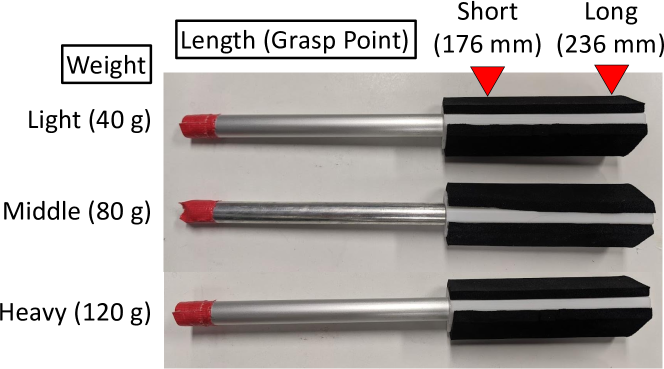
Figure 3: Six types of tool states with various weights and lengths used in this study.

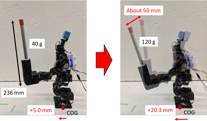
Figure 4: The change in tool-tip position and center of gravity when handling tools with different weights.

III-A Experimental Setup

In this study, we utilized a low-rigidity humanoid robot, KXR [4], made of plastic, as shown in Fig. 1. Three different tool weights (Light: 40 g, Middle: 80 g, Heavy: 120 g) were prepared, as depicted in Fig. 3. Additionally, based on the grasped positions of these tools, we defined two lengths (Short: 176 mm, Long: 236 mm), resulting in a total of six tool states. In Fig. 4, we illustrate the variations in the tool-tip position and center of gravity (COG) when holding tools of different weights. Even when using tools of the same length, due to the low rigidity of the hardware, there is a significant difference in the tool-tip position (about 50 mm) and the center of gravity position (about 15 mm) when holding a 40 g tool compared to a 120 g tool. Similarly, when the tool length changes, both the tool-tip position $\bm{x}_{tool}$ and screen coordinates $\bm{s}_{tool}$, as well as the center of gravity position $\bm{x}_{cog}$, change accordingly.

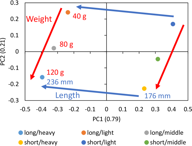
Figure 5: The trained parametric bias in the simulation experiment.

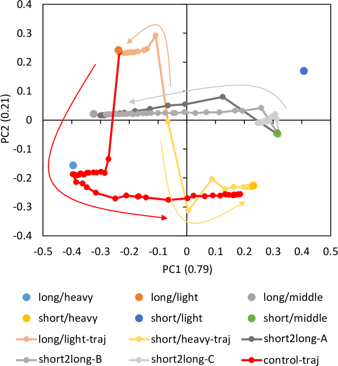
Figure 6: The trajectory of parametric bias during online update in the simulation experiment.

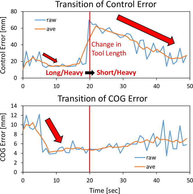
Figure 7: The transition of control and center of gravity errors in the simulation experiment.

III-B Simulation Experiment

The joint angle was randomly varied in a simulation, resulting in 500 data points for each tool state and a total of 3000 data points. The results of applying Principal Component Analysis (PCA) to PB obtained when training WTNPB using this data are shown in Fig. 5. It can be observed that each PB aligns neatly along the axes of tool weight and length.

Next, we demonstrate the accurate recognition of the current tool state through online update of PB. The tool was set to Long/Light or Short/Heavy states, and PB was updated online while sending random joint angles to the robot. The transitions of PB during this process are illustrated in Fig. 6 (long/light-traj and short/heavy-traj). It can be observed that the current PB values gradually approach the trained PB values for Long/Light or Short/Heavy. Additionally, we consider how online update is affected by data from different types of sensors obtained during operation. Regarding visual information, when an AR marker is attached to the tool tip, $\{\bm{x}_{tool},\bm{s}_{tool}\}$ can be obtained, but without an AR marker, only $\bm{s}_{tool}$ can be obtained based on color recognition. Furthermore, if the tool tip is not within the visual field, only the values $\{\bm{\theta},\bm{x}_{cog}\}$ can be obtained. Therefore, in this study, we examine how PB values transition in three scenarios of data availability, A: $\{\bm{\theta},\bm{x}_{cog},\bm{x}_{tool},\bm{s}_{tool}\}$, B: $\{\bm{\theta},\bm{x}_{cog},\bm{s}_{tool}\}$, and C: $\{\bm{\theta},\bm{x}_{cog}\}$. Here, we start from the trained PB for Short/Middle and investigate the case when handling the Long/Middle tool. The results are presented in Fig. 6. A (short2long-A) uses the same sensor types as the earlier long/light-traj and short/heavy-traj scenarios, so the PB quickly transitions and the tool state is accurately recognized. B (short2long-B) exhibits a slower transition compared to A, requiring more time to accurately perceive the tool state. C (short2long-C) shows that while the PB value is progressing in the correct direction, it has not reached the point of accurate recognition.

Finally, we conduct control experiments incorporating online update of PB. We initiate the current PB as Long/Light, and sequentially transition the actual tool states to Long/Heavy and Short/Heavy. It should be noted that in order to promptly adapt to tool changes, we set $N^{online}_{max}=5$. Random $\bm{x}^{ref}_{tool}$ values within the specified range are provided, and tool-tip control using WTNPB is executed to track these references. The transition of PB during this process is shown in Fig. 6 (control-traj). It can be observed that PB transitions from Long/Light to Long/Heavy and then to Short/Heavy as intended. The control error $||\bm{x}^{ref}_{tool}-\bm{x}_{tool}||_{2}$, center of gravity (COG) error $||\bm{x}^{ref}_{cog}-\bm{x}_{cog}||_{2}$, and their moving averages over five steps are shown in Fig. 7. Initially in the Long/Heavy state, we can see a slight reduction in control error and a significant decrease in COG error by the update of PB. In the subsequent transition to the Short/Heavy state, significant changes in control error are observed, while there is no significant variation in COG error.

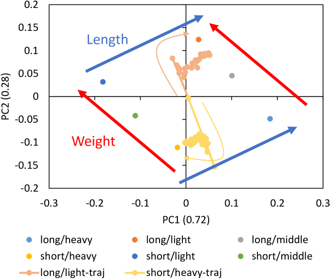
Figure 8: The trained parametric bias and the trajectory of the parametric bias during online update in the actual robot experiment.

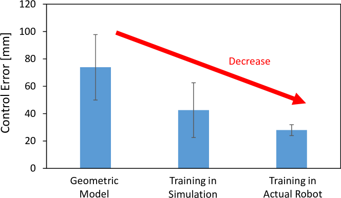
Figure 9: Comparison of control errors among the cases using a geometric model, using WTNPB after training with the simulation data, and using WTNPB after fine-tuning with the actual robot data, in the actual robot experiment.

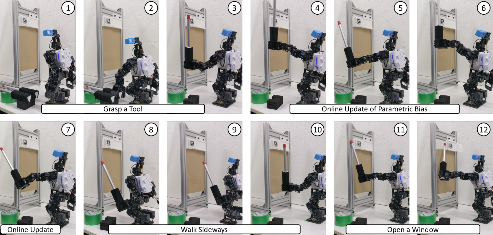
Figure 10: The integrated experiment of opening a window.

III-C Actual Robot Experiment

In this study, approximately 480 data points were obtained by collecting data with a GUI interface (60 data points) and with randomly specified joint angles (20 data points) while changing the tool states. The results of applying PCA to PB obtained during fine-tuning using this data are shown in Fig. 8. It is evident that each PB is self-organized neatly along the axes of tool weight and length.

Next, we demonstrate the ability to accurately recognize the current tool state through online update of PB. PB was updated online while setting the tool state to Long/Light or Short/Heavy, and sending random joint angles to the robot. The transitions of PB during this process are also shown in Fig. 8 (long/light-traj and short/heavy-traj). It can be observed that the current PB gradually approaches the trained PB of Long/Light or Short/Heavy.

Finally, an evaluation of control errors was conducted. We compared control errors for the Long/Middle tool state when solving whole-body inverse kinematics using a geometric model, when using WTNPB trained with the simulation data including joint deflection, and when using WTNPB fine-tuned with the actual robot data. The results comparing the average and variance of control errors for five $\bm{x}^{ref}_{tool}$ are shown in Fig. 9. It should be noted that PB used with WTNPB is the value obtained during training for Long/Middle. The geometric model exhibits the largest error, followed by training from the simulation data with joint deflection, and finally, the smallest control error is achieved after fine-tuning in the actual robot.

III-D Integrated Experiment

We conducted an integrated experiment that combined online update and tool-tip position control on the actual robot. The task involved using the tool to open a window located at a high position. We initiated the PB in the Short/Heavy state and the robot grasped the Long/Light tool. While performing random movements, the current PB was updated online and then the robot positioned itself in front of the window by walking sideways. The 3D position of the window was recognized from an AR marker attached to it. Subsequently, the robot extended the tool-tip position to the left of the window by 60 mm and then moved it 80 mm to the right to open the window. The entire sequence of actions was successful, demonstrating the feasibility of a series of tool manipulation tasks on a low-rigidity robot.

IV Discussion

We discuss the experimental results. First, both the simulation and actual robot experiments have revealed that the space of PB self-organizes regularly. Our learning method has demonstrated the implicit embedding of tool properties such as length and weight into the network through PB. It is also shown that the current tool state can be updated and understood from current sensor information. Moreover, the accuracy of online update depends significantly on the quantity and quality of available sensors, emphasizing the importance of collecting as many sensor data as possible for higher precision and faster convergence. Second, control experiments in a simulation demonstrated that online update of the tool state leads to improved control precision of the tool-tip position. Depending on the choice of the loss function, not only the tool-tip position but also the control of the center of gravity can be achieved, allowing for whole-body tool manipulation while maintaining balance. Third, actual robot experiments have highlighted the significance of fine-tuning with the actual robot data. Control accuracy improves sequentially with training from a geometric model that does not consider deflection, incorporating deflection into the geometric model with network training, and fine-tuning with the actual robot data. By combining these approaches, it has been demonstrated that even low-rigidity robots can perform whole-body tool-use considering visual and tactile sensor information.

We discuss the future prospects of this study. Currently, mask variables are arbitrarily determined by humans, but they should be automatically acquired by extracting correlations of sensors from experience. Furthermore, in robots equipped with numerous sensors, higher versatility can be achieved by automatically determining the input and output variables to be used. Also, while this study focused on a small humanoid robot, we anticipate that larger humanoid robots may face a variety of challenges. In particular, there is a need for deeper discussions on how to prevent falls and how to safely move the body randomly. In the future, we aim to eliminate human intervention and achieve robots with new levels of autonomy.

V CONCLUSION

In this study, we developed a method for a low-rigidity plastic-made humanoid to learn the mutual relationship among its joint angle, center of gravity, tool-tip position, and tool-tip screen coordinates, and to consider changes in the relationship due to variations in tool weight and length for whole-body robotic tool-use. To facilitate the learning of the mutual relationship, we introduced a mask variable to effectively capture correlations between four different modalities, enabling the robot to adapt to partial modality data loss during online update and control. By utilizing Parametric Bias as a learnable input variable, the internal network representation of weight and length variations for each tool is organized without explicit labeling, allowing the robot to estimate the tool state from current sensor information. We updated latent variables from loss functions related to visual and tactile information, enabling precise tool-tip position control while considering deflection and center of gravity changes. Moving forward, we aim to explore automatic construction of mask variables and network input-output variables, as well as conduct experiments with life-sized humanoids.

References

- [1] K. Hirai, M. Hirose, Y. Haikawa, and T. Takenaka, “The Development of Honda Humanoid Robot,” in Proceedings of the 1998 IEEE International Conference on Robotics and Automation, 1998, pp. 1321–1326.
- [2] K. Kaneko, F. Kanehiro, S. Kajita, H. Hirukawa, T. Kawasaki, M. Hirata, K. Akachi, and T. Isozumi, “Humanoid robot HRP-2,” in Proceedings of the 2004 IEEE International Conference on Robotics and Automation, 2004, pp. 1083–1090.
- [3] P. Allgeuer, H. Farazi, M. Schreiber, and S. Behnke, “Child-sized 3D printed igus humanoid open platform,” in Proceedings of the 2015 IEEE-RAS International Conference on Humanoid Robots, 2015, pp. 33–40.
- [4] T. Makabe, T. Anzai, Y. Kakiuchi, K. Okada, and M. Inaba, “Development of Amphibious Humanoid for Behavior Acquisition on Land and Underwater,” in Proceedings of the 2020 IEEE-RAS International Conference on Humanoid Robots, 2020, pp. 104–111.
- [5] C. Lee, M. Kim, Y. J. Kim, N. Hong, S. Ryu, H. J. Kim, and S. Kim, “Soft robot review,” International Journal of Control, Automation and Systems, vol. 15, no. 1, pp. 3–15, 2017.
- [6] C. T. Kiang, A. Spowage, and C. K. Yoong, “Review of Control and Sensor System of Flexible Manipulator,” Journal of Intelligent & Robotic Systems, vol. 77, no. 1, pp. 187–213, 2015.
- [7] C. Sun, W. He, and J. Hong, “Neural Network Control of a Flexible Robotic Manipulator Using the Lumped Spring-Mass Model,” IEEE Transactions on Systems, Man, and Cybernetics: Systems, vol. 47, no. 8, pp. 1863–1874, 2017.
- [8] J. Y. Loo, Z. Y. Ding, V. M. Baskaran, S. G. Nurzaman, and C. P. Tan, “Robust multimodal indirect sensing for soft robots via neural network-aided filter-based estimation,” Soft Robotics, vol. 9, no. 3, pp. 591–612, 2022.
- [9] G. Runge, M. Wiese, and A. Raatz, “FEM-based training of artificial neural networks for modular soft robots,” in Proceedings of the 2017 IEEE International Conference on Robotics and Biomimetics, 2017, pp. 385–392.
- [10] T. G. Thuruthel, B. Shih, C. Laschi, and M. T. Tolley, “Soft robot perception using embedded soft sensors and recurrent neural networks,” Science Robotics, vol. 4, no. 26, p. eaav1488, 2019.
- [11] J. Tani, “Self-organization of behavioral primitives as multiple attractor dynamics: a robot experiment,” in Proceedings of the 2002 International Joint Conference on Neural Networks, 2002, pp. 489–494.
- [12] K. P. Tee, J. Li, L. T. P. Chen, K. W. Wan, and G. Ganesh, “Towards Emergence of Tool Use in Robots: Automatic Tool Recognition and Use Without Prior Tool Learning,” in Proceedings of the 2018 IEEE International Conference on Robotics and Automation, 2018, pp. 6439–6446.
- [13] A. Xie, F. Ebert, S. Levine, and C. Finn, “Improvisation through Physical Understanding: Using Novel Objects as Tools with Visual Foresight,” arXiv preprint arXiv:1904.05538, 2019.
- [14] C. Nabeshima, Y. Kuniyoshi, and M. Lungarella, “Adaptive body schema for robotic tool-use,” Advanced Robotics, vol. 20, no. 10, pp. 1105–1126, 2006.
- [15] Y. Wu, K. Takahashi, H. Yamada, K. KIM, S. Murata, S. Sugano, and T. Ogata, “Dynamic Motion Generation by Flexible-Joint Robot based on Deep Learning using Images,” in Proceeding of the 8th Joint IEEE International Conference on Development and Learning on Epigenetic Robotics, 2018.
- [16] M. Eppe, P. D. H. Nguyen, and S. Wermter, “From Semantics to Execution: Integrating Action Planning With Reinforcement Learning for Robotic Causal Problem-Solving,” Frontiers in Robotics and AI, vol. 6, p. 123, 2019.
- [17] K. Fang, Y. Zhu, A. Garg, A. Kurenkov, V. Mehta, L. Fei-Fei, and S. Savarese, “Learning task-oriented grasping for tool manipulation from simulated self-supervision,” The International Journal of Robotics Research, vol. 39, no. 2-3, pp. 202–216, 2020.
- [18] K. Kawaharazuka, K. Okada, and M. Inaba, “Adaptive Robotic Tool-Tip Control Learning Considering Online Changes in Grasping State,” IEEE Robotics and Automation Letters, vol. 6, no. 3, pp. 5992–5999, 2021.
- [19] D. P. Kingma and J. Ba, “Adam: A Method for Stochastic Optimization,” in Proceedings of the 3rd International Conference on Learning Representations, 2015, pp. 1–15.