Extrinsic Bonnet-Myers Theorem and almost rigidity

Abstract.

We establish the extrinsic Bonnet-Myers Theorem for compact Riemannian manifolds with positive Ricci curvature. And we show the almost rigidity for compact hypersurfaces, which have positive sectional curvature and almost maximal extrinsic diameter in Euclidean space.
Mathematics Subject Classification: 53C21, 53A07, 52A20.

section[0em]  *[1pc]. subsection[1.5em]  *[1pc].

1. Introduction

The well-known Bonnet-Myers theorem says: for complete Riemannian manifold $(M^{n},g)$ with Ricci curvature $Rc\geq(n-1)$, the intrinsic diameter of $(M^{n},g)$ with respect to the Riemannian metric $g$ satisfies $\mathrm{Diam}_{g}(M^{n})\leq\pi$. Furthermore Cheng [Cheng] showed that the rigidity of Bonnet-Myers theorem, which says that $\mathrm{Diam}_{g}(M^{n})=\pi$ if and only if $(M^{n},g)$ is isometric to $\mathbb{S}^{n}$.

In the rest of this paper, unless otherwise mentioned, $(M^{n},g)$ is always a compact Riemannian manifold.

We use $\mathcal{IE}((M^{n},g),\mathbb{R}^{m})$ to denote the set of all smooth isometric embedding $\mathscr{I}:(M^{n},g)\rightarrow\mathbb{R}^{m}$, where $m\geq n+1$ and $n\geq 2$ are positive integers. From the well-known Nash’s isometric embedding theorem (see [Nash]), for any $(M^{n},g)$, there is $m\in\mathbb{Z}^{+}$ such that $\displaystyle\mathcal{IE}((M^{n},g),\mathbb{R}^{m})\neq\emptyset$.

For $\mathscr{I}\in\mathcal{IE}((M^{n},g),\mathbb{R}^{m})$, we define

$$\mathrm{Diam}_{\mathscr{I}}(M^{n},g)\vcentcolon=\sup_{x,y\in M^{n}}|\mathscr{I}(x)-\mathscr{I}(y)|_{\mathbb{R}^{m}}.$$

If $\mathcal{IE}((M^{n},g),\mathbb{R}^{m})\neq\emptyset$, we define the extrinsic diameter of $(M^{n},g)$ in $\mathbb{R}^{m}$ as follows:

$$\mathrm{Diam}_{\mathbb{R}^{m}}(M^{n},g)\vcentcolon=\sup_{\mathscr{I}\in\mathcal{IE}((M^{n},g),\mathbb{R}^{m})}\mathrm{Diam}_{\mathscr{I}}(M^{n},g).$$

Spruck [Spruck] showed: for any $(M^{n},g)$ with sectional curvature $K(g)\geq 1$ and $\mathscr{I}\in\mathcal{IE}((M^{n},g),\mathbb{R}^{n+1})$, there is $\mathrm{Diam}_{\mathscr{I}}(M^{n})<\pi$. A family of smooth examples was sketched in [Spruck] to show this upper bound is sharp. Those examples are spheres shrinking to a line segment with length $\pi$ in $\mathbb{R}^{n+1}$ (see Proposition 2.9 for details).

The first result of this paper is the following extrinsic Bonnet-Myers Theorem, which generalizes the above theorem of Spruck.

Theorem 1.1.

For complete Riemannian manifold $(M^{n},g)$ with $Rc\geq(n-1)$, we have

(1.1) $$\mathrm{Diam}_{\mathscr{I}}(M^{n},g)<\pi,\quad\quad\quad\forall\mathscr{I}\in\mathcal{IE}((M^{n},g),\mathbb{R}^{m}).$$

Furthermore (1.1) is sharp in the following sense: there exists a sequence of $(S^{n},g_{k})$ with $K(g_{k})\geq 1$ and $\mathscr{I}_{k}\in\mathcal{IE}((S^{n},g_{k})$, $\mathbb{R}^{n+1})$, such that $\displaystyle\lim_{k\rightarrow\infty}\mathrm{Diam}_{\mathscr{I}_{k}}(S^{n},g_{k})=\pi$.

Remark 1.2.

Although (1.1) is sharp in the above sense; for complete Riemannian manifold $(M^{n},g)$ with $Rc\geq(n-1)$ and $m\geq n+1$, we currently do not know whether $\mathrm{Diam}_{\mathbb{R}^{m}}(M^{n},g)<\pi$ generally holds or not. However, Theorem 1.4 provides partial result when $K\geq 1$ and $m=n+1$.

From the rigidity part of Bishop-Gromov’s volume comparison Theorem, for complete Riemannian manifold $(M^{n},g)$ with $Rc(g)\geq(n-1)$, we have $V(M^{n})=V(\mathbb{S}^{n})$ if and only if $M^{n}$ is isometric to $\mathbb{S}^{n}$. Furthermore, there is almost rigidity with respect to almost maximal volume in the above context. To explain it, we recall some concepts as follows.

For two subsets $A,B$ of a metric space $Z$, the Hausdorff distance between $A$ and $B$ among $Z$ is

$$d_{H}^{Z}(A,B)=\inf\big{\{}\epsilon>0:B\subset\mathbf{U}_{\epsilon}(A)\ and\ A\subset\mathbf{U}_{\epsilon}(B)\big{\}}$$

where $\displaystyle\mathbf{U}_{\epsilon}(A)\vcentcolon=\big{\{}z\in Z:d_{Z}(z,A)\leq\epsilon\big{\}}$. The Gromov-Hausdorff distance (also see [Gromov-book]) between two metric space $X,Y$, is denoted as $d_{GH}(X,Y)$,

$$d_{GH}(X,Y)=\inf_{\mathscr{I}_{1}\in\mathscr{IE}(X,Z)\atop\mathscr{I}_{2}\in\mathscr{IE}(Y,Z)}d_{H}^{Z}\big{(}\mathscr{I}_{1}(X),\mathscr{I}_{2}(Y)\big{)}$$

where $Z$ is any metric space with non-empty $\mathscr{IE}(X,Z)$ and $\mathscr{IE}(Y,Z)$; and $\mathscr{IE}(X,Z)$ is the set of all isometric embedding of $X$ into $Z$, similarly $\mathscr{IE}(Y,Z)$ is defined. If $d_{GH}\big{(}(X,d_{X}),(Y,d_{Y})\big{)}\leq\epsilon$, we say that $(X,d_{X})$ is $\epsilon$-Gromov-Hausdorff close to $(Y,d_{Y})$.

Remark 1.3.

The set $\mathcal{IE}((M^{n},g),\mathbb{R}^{m})$ contains only smooth isometric embeddings, which not only keep the distance property but also preserve the property of Riemannian manifolds’ curvature. On the other hand, the set $\mathscr{IE}(X,Z)$ contains all isometric embeddings between two metric spaces $X,Z$; which is only distance-preserving (comparing [Nash-C1]).

Colding [Colding-shape], [Colding-large] (also see [WZ]) proved the almost rigidity of Bishop-Gromov’s volume comparison Theorem. More concretely, he showed that $(M^{n},g)$ with $Rc\geq(n-1)$, is Gromov-Hausdorff close to $\mathbb{S}^{n}$, if and only if the volume of $(M^{n},g)$ is almost maximal (i.e. is close to the volume of $\mathbb{S}^{n}$).

Note the model space with respect to almost maximal volume is $\mathbb{S}^{n}$.

On the other hand, there is no almost rigidity for almost maximal intrinsic diameter, although there is Cheng’s rigidity theorem of maximal diameter [Cheng]. There are round spheres with almost maximal intrinsic diameter and ‘needle type’ convex spheres (see examples in Proposition 2.9), both of them have almost intrinsic maximal diameter; but they are not Gromov-Hausdorff close to each other.

However, with respect to the extrinsic diameter, we have the following almost rigidity theorem with the collapsing model $[0,\pi]$.

Theorem 1.4.

For complete Riemannian manifold $(M^{n},g)$ with $K(g)\geq 1$ and $\displaystyle\mathcal{IE}((M^{n},g),\mathbb{R}^{n+1})\neq\emptyset$, we have

$$\frac{d_{GH}((M^{n},g),[0,\pi])}{\sqrt{\pi-\mathrm{Diam}_{\mathbb{R}^{n+1}}(M^{n},g)}}\leq 4\pi^{\frac{3}{2}}.$$

Remark 1.5.

If the assumption $K(g)\geq 1$ is replaced by $Rc(g)\geq n-1$, where $n\geq 3$, we do not know whether the above conclusion is true or not.

The organization of this paper is as follows. We prove the extrinsic Bonnet-Myers Theorem (Theorem 1.1) in Section 2. Specially, the examples showing the sharpness of extrinsic diameter upper bound, is constructed in details. And the sharp bound is obtained through applying the Cheng’s rigidity Theorem for Bonnet-Myers’ Theorem. The assumption of this section is $Rc\geq(n-1)$, and there is not restriction on the co-dimension of isometric embeddings.

In Section 3, using Toponogov’s comparison Theorem, some facts of Euclidean geometry and spherical geometry, we estimate the height of Euclidean triangles in term of the gap between sharp upper bound and extrinsic diameter of manifolds, where the vertexes of those Euclidean triangles are in the image of isometric embedded Riemannian manifolds in Euclidean spaces. Sectional curvature $K(g)\geq 1$ is needed in this section. The results of this section imply that the isometric embedding image of Riemannian manifolds with almost maximal extrinsic diameter lies in an Euclidean neighborhood of a line segment in the ambient Euclidean space. The final main estimate obtained in this section can be viewed as the upper bound of ‘extrinsic width’ of manifolds isometrically embedded into $\mathbb{R}^{m}$.

Finally, on manifolds with almost maximal extrinsic diameter, we consider ‘height function’, which is the projection map onto the line segment corresponding to the extrinsic diameter. We show the intrinsic diameter’s upper bound of the level set of ‘height function’. This will be obtained by the convexity of isometric embedding image of manifolds and the ‘extrinsic width estimate’ obtained in Section 3. The convexity relies on the co-dimension of isometric embedding equal to $1$. Then we show that the map (which maps the interval to the geodesic segment linking the end points of extrinsic diameter) is a Gromov-Hausdorff approximation, with respect to the scale of the gap between extrinsic diameter and its sharp upper bound. Combining the relationship between Gromov-Hausdorff approximation and Gromov-Hausdorff distance, we get the almost rigidity.

2. The extrinsic Bonnet-Myers Theorem

We fix some notations, which will be used repeatedly in the rest of the paper.

Notation 2.1.

For any curve $\gamma\subseteq(M^{n},g)$, we use $\ell(\gamma)$ to denote the length of the curve $\gamma$. For $p,q\in(M^{n},g)$, we use $\gamma_{p,q}$ to denote one geodesic segment from $p$ to $q$ in $(M^{n},g)$. Then $\ell(\gamma_{p,q})=d_{g}(p,q)$.

For distinct points $x,y\in\mathbb{R}^{m}$, we use $l_{x,y}$ to denote the line passing $x,y$ and $\overline{xy}$ to denote the line segment from $x$ to $y$. We use $|x-y|$ or $|x-y|_{\mathbb{R}^{m}}$ to denote the Euclidean length of $\overline{xy}$.

In this section, for any $\epsilon\in(0,\pi)$, we firstly construct a smooth Riemannian manifold $(S^{n},g)\subset\mathbb{R}^{n+1}$ with $K(g)\geq 1$, and some $\mathscr{I}\in\mathcal{IE}((S^{n},g),\mathbb{R}^{n+1})$, such that $\mathrm{Diam}_{\mathscr{I}}(S^{n},g)\geq\pi-\epsilon$. Then we prove the extrinsic Bonnet-Myers Theorem, whose sharpness is guaranteed by the example in Proposition 2.9.

For $(S^{n},g)$ with normal coordinate chart $\{t,\theta_{1},...,\theta_{n-1}\}$ and metric $g=dt^{2}+f^{2}(t)d\theta^{2}$, where $d\theta=d\theta_{1}d\theta_{2}...d\theta_{n-1}$ is the canonical measure on $\mathbb{S}^{n-1}$, we select an orthonormal basis $\{E_{i}\}$ where $E_{1}=\frac{\partial}{\partial t}$, for all $X,Y=E_{i}$ where $i\neq 1$. The sectional curvatures are as follows:

(2.1) $$K(E_{1},X)=-\frac{f^{\prime\prime}}{f},\quad\quad K(X,Y)=\frac{1-(f^{\prime})^{2}}{f^{2}},\quad\quad\forall X\neq Y.$$

The following lemma is well-known (see [PP]).

Lemma 2.2.

If $f:[c,b]\rightarrow[0,\infty)$ is smooth and $f(c)=0$, the metric of $(S^{n},g)$ is $g=dt^{2}+f^{2}(t)d\theta^{2}$, then $g$ is smooth at $t=c$ if and only if

$$f^{\prime}(c)=1,\quad\quad f^{(even)}(c)=0.$$

∎

According to [Spruck], the example manifold (see Proposition 2.9) was pointed out by Calabi. We provide a detailed construction of the example for completeness reason.

Remark 2.3.

There are two key points of the construction of example manifolds in Proposition 2.9. The first one is define the twisted factor $f(t)$ as the solution of ODE (2.6); and this ODE comes from the curvature term $-\frac{f^{\prime\prime}}{f}\geq 1$. Therefore we reduce the construction of the metric to the choice of suitable function $h$ in (2.6).

The second idea is: to solve $f$ with standard initial data at starting point $t=0$, and get the upper bound of $f^{\prime}(c)$ where $t=c$ is another end point; then scaling the metric by $|f^{\prime}(c)|^{-1}$, to guarantee the smoothness of the metric obtained by the new function $\tilde{f}$.

Lemma 2.4.

For any $k\geq 100$, there exists $(S^{n},g_{f})$ with $\displaystyle g_{f}=dt^{2}+f^{2}(t)d\theta^{2},t\in[-c,c]$, where $c\geq\frac{\pi}{2}-\frac{1}{k}+\frac{1}{4k^{2}}$ and $f$ is an even function; such that $(S^{n},g_{f})$ is smooth except two points with $t=\pm c$, and

$$K(g_{f})\geq 1,\quad\quad\quad\forall t\in[-\frac{\pi}{2}+\frac{1}{k},\frac{\pi}{2}-\frac{1}{k}],$$

(2.2) $$f^{(even)}(\pm c)=0,\quad\quad\quad|f^{\prime}(\pm c)|\geq\frac{3k}{16},$$

$$f^{\prime\prime}(t)+f(t)\leq 0,\quad\quad f^{2}(t)+(f^{\prime})^{2}(t)-(f^{\prime}(c))^{2}\leq 0,\quad\quad\quad\forall t\in[-c,c].$$

Remark 2.5.

Because of (2.2) and Lemma 2.2, we know that $g_{f}$ is not a smooth metric at $t=\pm c$.

From our argument below, the sectional curvature $K(g_{f})\geq 0$ does not hold on $(S^{n},g_{f})$ for all $t\in(-c,c)$, because $1-|f^{\prime}(t)|^{2}<0$ for $t$ is close to $\pm c$.

Proof: Step (1). We define the smooth function $\varphi(t)\vcentcolon=\frac{\int_{-\infty}^{t}F(s)ds}{\int_{-\infty}^{\infty}F(s)ds}$, where

(2.5) $$F(t)\vcentcolon=\left\{\begin{array}[]{rl}e^{\frac{1}{t(t-1)}},0<t<1,\\ 0,\quad\text{otherwise}.\end{array}\right.$$

Denote $c_{0}=\frac{1}{4}$ and $\delta=\frac{c_{0}}{4}=\frac{1}{16}$ in the rest argument. Now we define a smooth function $h:[0,\frac{\pi}{2}]\rightarrow\overline{\mathbb{R}^{-}}$ as follows (see Figure 1):

$$h(t)=\left\{\begin{array}[]{rl}&\varphi(\frac{t-(\frac{\pi}{2}-\frac{1}{k})}{k^{-2}\delta})\cdot\Big{(}-\delta^{-1}k^{5}\cdot(t-\frac{\pi}{2}+\frac{1}{k})\Big{)}\ ,\quad\quad\quad\quad t\in[0,\frac{\pi}{2}-\frac{1}{k}+\frac{3}{2}\cdot\frac{\delta}{k^{2}}],\\ &\Big{(}1-\varphi(\frac{t-(\frac{\pi}{2}-\frac{1}{k}+2\frac{\delta}{k^{2}})}{k^{-2}\delta})\Big{)}\cdot\Big{(}-\delta^{-1}k^{5}\cdot(t-\frac{\pi}{2}+\frac{1}{k})\Big{)}\ ,\quad\quad t\in[\frac{\pi}{2}-\frac{1}{k}+\frac{3}{2}\cdot\frac{\delta}{k^{2}},\frac{\pi}{2}].\end{array}\right.$$

Figure 1. The figure of h(t)

We assume $f$ is the solution to the following $2$nd order ODE:

(2.6) $$f^{\prime\prime}(t)+f(t)=h(t),\quad\quad f(0)=1,\quad\quad f^{\prime}(0)=0,\quad\quad\quad t\in[0,\frac{\pi}{2}].$$

Note $k\geq 100$, since $f^{\prime\prime}<0$ in $[0,\frac{\pi}{2}-\frac{1}{k}]$ and $f^{\prime}(0)=0$, then $f^{\prime}(t)$ is decreasing and less than a negative number when $t\in(\frac{\pi}{2}-\frac{1}{k},\frac{\pi}{2})$. So $f$ decreases to 0 in finite time $[0,c]$. From Bonnet-Myers theorem, $c\in(\frac{\pi}{2}-\frac{1}{k},\frac{\pi}{2})$. Now we have $f(c)=0$ and $f(t)>0$ for any $t\in(0,c)$ (see Figure 2).

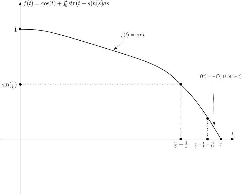
Figure 2. The figure of f(t)

Step (2). From the uniqueness of solution to ODE, we know that $f(t)=\cos t$ for any $t\in[0,\frac{\pi}{2}-\frac{1}{k}]$. Now on $[\frac{\pi}{2}-\frac{1}{k},c)$, we have

$$f^{\prime\prime}(t)=-f(t)+h(t)\geq-\sin(\frac{1}{k})-3k^{3}$$

Then for $t\in[\frac{\pi}{2}-\frac{1}{k},c)$, we get

$$f^{\prime}(t)=f^{\prime}(\frac{\pi}{2}-\frac{1}{k})+\int_{\frac{\pi}{2}-\frac{1}{k}}^{t}f^{\prime\prime}(s)ds\geq-1-(\sin(\frac{1}{k})+3k^{3})\cdot(t-[\frac{\pi}{2}-\frac{1}{k}]).$$

By Newton-Leibniz formula again, let $\tilde{t}=t-[\frac{\pi}{2}-\frac{1}{k}]$, we get

$$f(t)=f(\frac{\pi}{2}-\frac{1}{k})+\int_{\frac{\pi}{2}-\frac{1}{k}}^{t}f^{\prime}(s)ds\geq\sin(\frac{1}{k})-\tilde{t}-\frac{\tilde{t}^{2}}{2}(\sin(\frac{1}{k})+3k^{3}).$$

If $\displaystyle 0\leq\tilde{t}<\frac{-1+\sqrt{1+2\sin(\frac{1}{k})(\sin(\frac{1}{k})+3k^{3})}}{\sin(\frac{1}{k})+3k^{3}}$, we have $f(t)>0$.

For any $k\geq 1$, using $\frac{\sin x}{x}\in[\frac{2}{\pi},2]$ where $x\in(0,\frac{\pi}{2})$, we obtain

$$\frac{-1+\sqrt{1+2\sin(\frac{1}{k})(\sin(\frac{1}{k})+3k^{3})}}{\sin(\frac{1}{k})+3k^{3}}k^{2}\geq\frac{-1+\sqrt{1+2\cdot\frac{2}{\pi}\cdot\frac{1}{k}\cdot 3k^{3}}}{1+3k^{3}}k^{2}$$

$$\geq\frac{-1+2k}{1+3k}\geq\frac{1}{4}=c_{0}.$$

Therefore $f(t)>0$ if $\tilde{t}\leq c_{0}k^{-2}$, and

(2.7) $$c\geq(\frac{\pi}{2}-\frac{1}{k})+c_{0}k^{-2}=\frac{\pi}{2}-\frac{1}{k}+\frac{4\delta}{k^{2}}.$$

By the definition of $h(t),$ we have $h^{(m)}(c)=0$, for any $m\in\mathbb{N}.$ So $f^{\prime\prime}(c)+f(c)=h(c)=0.$ Since $f(c)=0$, then $f^{\prime\prime}(c)=0.$ By $f^{(m+2)}(c)+f^{(m)}(c)=h^{(m)}(c)$, we have $f^{(even)}(c)=0.$

For any $t\in[0,c]$, using Newton-Leibniz formula and $f(c)=0,f^{\prime\prime}(s)=h(s)-f(s),f^{\prime}(s)\leq 0$, we have

$$f^{2}(t)+(f^{\prime})^{2}(t)-(f^{\prime}(c))^{2}=f^{2}(t)-f^{2}(c)-\int_{t}^{c}2f^{\prime}(s)f^{\prime\prime}(s)ds$$

(2.8) $$=\int_{c}^{t}2f(s)f^{\prime}(s)+2f^{\prime}(s)f^{\prime\prime}(s)ds=-\int_{t}^{c}2f^{\prime}(s)h(s)ds\leq 0.$$

By the decreasing property of $f^{\prime}$ on $(0,c)$, we get

$$f^{\prime}(c) \leq f^{\prime}((\frac{\pi}{2}-\frac{1}{k})+c_{0}k^{-2})=f^{\prime}(\frac{\pi}{2}-\frac{1}{k})+\int_{\frac{\pi}{2}-\frac{1}{k}}^{(\frac{\pi}{2}-\frac{1}{k})+c_{0}k^{-2}}f^{\prime\prime}(s)ds$$

(2.9) $$\leq\int_{\frac{\pi}{2}-\frac{1}{k}+\delta\cdot k^{-2}}^{(\frac{\pi}{2}-\frac{1}{k})+4\delta k^{-2}}-k^{3}ds=-3\delta k.$$

∎

Remark 2.6.

To “round off” those two singularities $t=\pm c$, we only need to scale metric on $d\theta^{2}$ factor by $\frac{1}{|f^{\prime}(c)|}=\frac{1}{|f^{\prime}(-c)|}$; which is done in the argument of Proposition 2.9.

Lemma 2.7.

For a smooth function $f:[-c,c]\rightarrow\mathbb{R}$ with

$$f\big{|}_{(-c,c)}>0,\quad\quad|f^{\prime}|\leq 1,\quad\quad f^{(even)}(\pm c)=0,\quad\quad f^{\prime}(\pm 1)=0;$$

define a Riemannian manifold $(S^{n},g_{f})$ with $g_{f}=dt^{2}+f^{2}(t)d\theta^{2}$, where $t\in[-c,c]$, $d\theta^{2}$ is the canonical metric of $\mathbb{S}^{n-1}$, and $\theta_{1},\cdots,\theta_{n-2}\in[0,\pi],\theta_{n-1}\in[0,2\pi]$ is the coordinate system of $\mathbb{S}^{n-1}$. Then there is $\mathscr{I}_{f}\in\mathcal{IE}((S^{n},g),\mathbb{R}^{n+1})$, where

$$\mathscr{I}_{f}(t,\theta_{1},\cdots,\theta_{n-1})$$

$$=(f(t)\cos\theta_{1},f(t)\sin\theta_{1}\cos\theta_{2},...,f(t)\cos\theta_{n-1}\prod_{i=1}^{n-2}\sin\theta_{i},$$

$$\quad\quad f(t)\sin\theta_{n-1}\prod_{i=1}^{n-2}\sin\theta_{i},\int_{0}^{t}\sqrt{1-f^{\prime 2}(s)}ds).$$

Proof: It is trivial. ∎

Remark 2.8.

Some part of the Riemannian manifold $(S^{n},g_{f})$ (from Lemma 2.4) with $|f^{\prime}|>1$, can not be isometrically embedded into $\mathbb{R}^{n+1}$ by the isometric embedding $\mathscr{I}$ in Lemma 2.7.

Proposition 2.9.

For any $\epsilon>0,$ there exists a smooth hypersurface $(S^{n},g)$ with $K(g)\geq 1$ with $\mathscr{I}\in\mathcal{IE}((S^{n},g),\mathbb{R}^{n+1})$, such that $\mathrm{Diam}_{\mathscr{I}}(S^{n},g)\geq\pi-\epsilon$ .

Proof: For $k\geq 100$ to be determined later, choose $f$ from Lemma 2.4, let $\tilde{f}(t)=\frac{f(t)}{|f^{\prime}(c)|}:[-c,c]\rightarrow\mathbb{R}$, then

(2.10) $$\tilde{f}^{\prime\prime}+\tilde{f}\leq 0,\quad\tilde{f}^{2}+(\tilde{f}^{\prime})^{2}-1\leq 0,$$

(2.11) $$\tilde{f}(0)=\frac{1}{|f^{\prime}(c)|},\quad\tilde{f}^{\prime}(0)=0,\quad\tilde{f}(c)=0,\quad\tilde{f}^{\prime}(c)=-1,\quad\tilde{f}^{(even)}(c)=0.$$

Consider $(S^{n},g_{\tilde{f}})\subseteq\mathbb{R}^{n+1}$ defined by $\tilde{f}$ as in Lemma 2.7, where $g_{\tilde{f}}=dt^{2}+\tilde{f}^{2}(t)d\theta^{2}$. Then $g_{\tilde{f}}$ is smooth by (2.11) and Lemma 2.2 (see Figure 3, where $|f^{\prime}(\pm t_{0})|=1$).

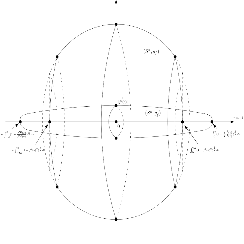
Figure 3. Scaling the slice spheres to smooth the two ends singularities

From (2.10) and (2.1), we get that $K(g_{\tilde{f}})\geq 1$. From $\tilde{f}^{\prime\prime}\leq 0,\tilde{f}^{\prime}(0)=0$, there is $-1\leq\tilde{f}^{\prime}\big{|}_{[0,c]}\leq 0$. Using (2.7) and (2.9), we have

$$\mathrm{Diam}_{\mathscr{I}_{\tilde{f}}}(S^{n},g_{\tilde{f}}) \geq 2\int_{0}^{c}\sqrt{1-\tilde{f}^{\prime 2}(s)}ds\geq 2\int_{0}^{c}1+\tilde{f}^{\prime}(s)ds=2c-2\tilde{f}(0)$$

$$\geq\pi-\frac{2}{k}-\frac{2}{|f^{\prime}(c)|}\geq\pi-\frac{20}{k}.$$

If $k$ is big enough, we get that $\mathrm{Diam}_{\mathscr{I}_{\tilde{f}}}(S^{n},g_{\tilde{f}})>\pi-\epsilon$, the conclusion is proved. ∎

Theorem 2.10.

For complete Riemannian manifold $(M^{n},g)$ with $Rc\geq(n-1)$, we have

(2.12) $$\mathrm{Diam}_{\mathscr{I}}(M^{n},g)<\pi,\quad\quad\quad\forall\mathscr{I}\in\mathcal{IE}((M^{n},g),\mathbb{R}^{m}).$$

Furthermore (2.12) is sharp in the following sense: there exists a sequence of $(S^{n},g_{k})$ with $K(g_{k})\geq 1$ with $\mathscr{I}_{k}\in\mathcal{IE}((S^{n},g_{k}),\mathbb{R}^{n+1})$ and $\displaystyle\lim_{k\rightarrow\infty}\mathrm{Diam}_{\mathscr{I}_{k}}(S^{n},g_{k})=\pi$.

Proof: We prove (2.12) by contradiction, assume $\mathrm{Diam}_{\mathscr{I}}(M^{n},g)=\pi$ for some $\mathscr{I}\in\mathcal{IE}((M^{n},g),\mathbb{R}^{m})$.

From Bonnet-Myers’ Theorem and $Rc(g)\geq n-1$, we have

$$\mathrm{Diam}_{g}(M^{n})\leq\pi.$$

Therefore $\mathrm{Diam}_{\mathscr{I}}(M^{n},g)\leq\mathrm{Diam}_{g}(M^{n})\leq\pi$.

By $\mathrm{Diam}_{\mathscr{I}}(M^{n},g)=\pi$, we have $\mathrm{Diam}_{g}(M^{n})=\pi.$ Assume for $p,q\in M^{n}$, we have

$$|\mathscr{I}(p)-\mathscr{I}(q)|_{\mathbb{R}^{m}}=\pi.$$

Denote the unit speed geodesic segment from $\mathscr{I}(p)$ to $\mathscr{I}(q)$ in $(\mathscr{I}(M^{n}),g)$ as $\gamma_{\mathscr{I}(p),\mathscr{I}(q)}$. If $\gamma_{\mathscr{I}(p),\mathscr{I}(q)}$ is not a line segment in $\mathbb{R}^{m}$, then

$$d_{g}(p,q)=d_{g}(\mathscr{I}(p),\mathscr{I}(q))>|\mathscr{I}(p)-\mathscr{I}(q)|_{\mathbb{R}^{m}}=\pi.$$

This contradicts $\mathrm{Diam}_{g}(M^{n})=\pi.$ So $\gamma_{\mathscr{I}(p),\mathscr{I}(q)}$ is a line segment in $\mathbb{R}^{m}$.

Assume $\tilde{\nabla}$ is the Levi-Civita connection of $\mathbb{R}^{m}$, $\nabla$ is the Levi-Civita connection of $(M^{n},g)$. For simplicity, we use $\gamma$ to denote $\gamma_{\mathscr{I}(p),\mathscr{I}(q)}$ in the rest argument.

Choose the parallel unit orthogonal frame $\{e_{i}\}_{i=1}^{n}$ along $\gamma(t)$ with $e_{1}=\gamma^{\prime}(t)$. By Gauss equation, for $2\leq i\leq n$, we have

(2.13) $$\widetilde{Rm}(e_{1},e_{i},e_{1},e_{i})=Rm(e_{1},e_{i},e_{1},e_{i})-\langle S(e_{1},e_{1}),S(e_{i},e_{i})\rangle+|S(e_{1},e_{i})|^{2},$$

where $\widetilde{Rm}$ is the Riemannian curvature of $\mathbb{R}^{m}$, $Rm$ is the Riemannian curvature of $(M^{n},g),$ $S(X,Y)=-(\tilde{\nabla}_{X}Y)^{\perp}$ is the second fundamental form of $(M^{n},g)\subseteq\mathbb{R}^{m}$.

Since $\gamma(t)$ is a line segment in $\mathbb{R}^{m}$, we have $\tilde{\nabla}_{e_{1}}e_{1}=0$, then $S(e_{1},e_{1})=0.$ Now from (2.13) and $\widetilde{Rm}=0$, we get

(2.14) $$Rc(e_{1},e_{1})=\sum\limits_{i=2}^{n}Rm(e_{1},e_{i},e_{1},e_{i})=\sum\limits_{i=2}^{n}-|S(e_{1},e_{i})|^{2}\leq 0$$

which contradicts $Rc(g)\geq(n-1).$

Hence $\mathrm{Diam}_{\mathscr{I}}(M^{n},g)<\pi.$ The sharpness of (2.12) follows from Proposition 2.9. ∎

3. The height of triangles

A geodesic hinge $(c_{1},c_{0},\alpha)$ in $(M^{n},g)$ consists of two nonconstant geodesic segments $c_{1},c_{0}$ with the same initial point making the angle $\alpha$. A geodesic segment $c_{2}$ between the endpoints of $c_{1}$ and $c_{0}$ is called a closing edge of the hinge. We recall the Toponogov’s theorem (see [CE]) as follows.

Theorem 3.1 (Toponogov).

Let $(M^{n},g)$ be a complete Riemannian manifold with $K(g)\geq 1$. Let $(c_{0},c_{1},\alpha)$ be a hinge in $M$ and $c$ a closing edge. Then the closing edge $\tilde{c}$ of any hinge $(\tilde{c}_{0},\tilde{c}_{1},\alpha)$ in $\mathbb{S}^{n}$ with $\ell(\tilde{c}_{i})=\ell(c_{i}),i=0,1$, satisfies $\ell(\tilde{c})\geq\ell(c)$.

∎

Recall the excess function defined in [AG] as follows.

Definition 3.2.

For $p,q\in(M^{n},g)$, we define the excess function with respect to $p,q$, denoted as $\mathbf{E}_{p,q}:M^{n}\rightarrow\mathbb{R}$, as:

$$\mathbf{E}_{p,q}(x)=d_{g}(p,x)+d_{g}(q,x)-d_{g}(p,q).$$

Lemma 3.3.

For complete Riemannian manifold $(M^{n},g)$ with $K(g)\geq 1$, we have

$$\sup_{x\in M^{n}}\mathbf{E}_{p,q}(x)\leq 2(\pi-d_{g}(p,q)),\quad\quad\quad\forall p,q\in M^{n}.$$

Proof: Applying Toponogov Theorem on hinges $\{\gamma_{x,p},\gamma_{x,q},\alpha\}\subseteq(M^{n},g)$, we can find a spherical triangle $\{\gamma_{\tilde{x},\tilde{p}},\gamma_{\tilde{x},\tilde{q}},\alpha\}\subseteq\mathbb{S}^{n}$, where $\alpha$ are angles between geodesic segments $\gamma_{x,p},\gamma_{x,q}$ and

$$d_{g}(p,x)=d_{\mathbb{S}^{n}}(\tilde{p},\tilde{x}),\quad\quad d_{g}(q,x)=d_{\mathbb{S}^{n}}(\tilde{q},\tilde{x}),\quad\quad d_{\mathbb{S}^{n}}(\tilde{p},\tilde{q})\geq d_{g}(p,q).$$

From spherical geometry, we know that

$$d_{\mathbb{S}^{n}}(\tilde{p},\tilde{x})+d_{\mathbb{S}^{n}}(\tilde{q},\tilde{x})\leq 2\pi-d_{\mathbb{S}^{n}}(\tilde{p},\tilde{q}).$$

Using $d_{\mathbb{S}^{n}}(\tilde{p},\tilde{q})\geq d_{g}(p,q)$, then

$$\mathbf{E}_{p,q}(x)=d_{g}(p,x)+d_{g}(q,x)-d_{g}(p,q)=d_{\mathbb{S}^{n}}(\tilde{p},\tilde{x})+d_{\mathbb{S}^{n}}(\tilde{q},\tilde{x})-d_{g}(p,q)$$

$$\leq 2\pi-d_{\mathbb{S}^{n}}(\tilde{p},\tilde{q})-d_{g}(p,q)\leq 2\pi-2d_{g}(p,q).$$

∎

Lemma 3.4.

For any triangle $\triangle abc\subseteq\mathbb{R}^{2}$, we have

$$d(a,l_{b,c})^{2}\leq\frac{(|b-a|+|c-a|)^{2}-|b-c|^{2}}{4}.$$

Proof: Assume $\overline{aa_{0}}\perp l_{b,c}$, where $a_{0}\in l_{b,c}$ (note $a_{0}$ possibly does not belong to $\overline{bc}$). Then $d(a,l_{b,c})=|a-a_{0}|$ (see Figure 4). Now from the Cosine Law

$$d(a,l_{b,c})^{2} =\frac{1}{|b-c|^{2}}(\frac{(|b-a|+|c-a|)^{2}-|b-c|^{2}}{2})\cdot(\frac{|b-c|^{2}-(|b-a|-|c-a|)^{2}}{2})$$

$$\leq\frac{(|b-a|+|c-a|)^{2}-|b-c|^{2}}{4}.$$

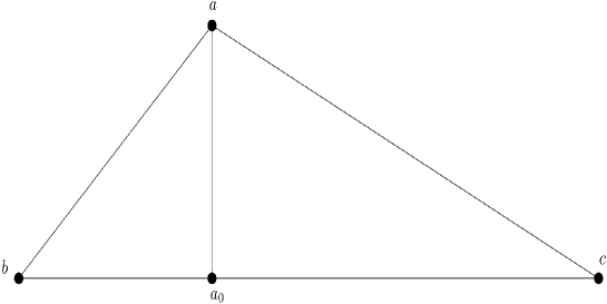
Figure 4. The Triangle

∎

Now we show the height estimate of an Euclidean triangle, whose vertexes are in the image of $\mathscr{I}(M^{n})$, where $(M^{n},g)$ has $K(g)\geq 1$ and $\mathscr{I}\in\mathcal{IE}((M^{n},g),\mathbb{R}^{m})$.

Proposition 3.5.

For complete Riemannian manifold $(M^{n},g)$ with $K(g)\geq 1$ and $m\geq n+1$, assume $p,q\in M^{n}$. Then

(3.1) $$\sup_{a\in M^{n}}\frac{d_{\mathbb{R}^{m}}(\mathscr{I}(a),l_{\mathscr{I}(p),\mathscr{I}(q)})}{\sqrt{\pi-|\mathscr{I}(p)-\mathscr{I}(q)|_{\mathbb{R}^{m}}}}\leq\sqrt{\pi},\quad\quad\quad\forall\mathscr{I}\in\mathcal{IE}((M^{n},g),\mathbb{R}^{m}).$$

Remark 3.6.

If $\mathrm{Diam}_{\mathscr{I}}(M^{n},g)=\pi-\epsilon$ for some positive $\epsilon<<1$, choose $p,q$ such that $|\mathscr{I}(p)-\mathscr{I}(q)|_{\mathbb{R}^{m}}=\pi-\epsilon$; then Proposition 3.5 gives the “extrinsic width” estimates for $\mathscr{I}(M^{n})\subseteq\mathbb{R}^{m}$.

Proof: Assume $|\mathscr{I}(p)-\mathscr{I}(q)|_{\mathbb{R}^{m}}=\pi-\epsilon$, where $\epsilon>0$. Assume $d_{g}(p,q)=\pi-\delta$, then $\delta\leq\epsilon$. By Lemma 3.3, we get

$$\sup_{x\in M^{n}}\mathbf{E}_{p,q}(x)+d_{g}(p,q)\leq 2\pi-d_{g}(p,q)=\pi+\delta\leq\pi+\epsilon.$$

Consider the Euclidean triangle $\Delta\mathscr{I}(p)\mathscr{I}(a)\mathscr{I}(q)\subseteq\mathbb{R}^{m}$ with $\overline{\mathscr{I}(a)b}\perp l_{\mathscr{I}(p),\mathscr{I}(q)}$, where $b\in l_{\mathscr{I}(p),\mathscr{I}(q)}$. We define $h\vcentcolon=|\mathscr{I}(a)-b|$ (see Figure 5), then from Lemma 3.4 and Lemma 3.3, we obtain

$$h^{2} \leq\frac{(|\mathscr{I}(p)-\mathscr{I}(a)|+|\mathscr{I}(q)-\mathscr{I}(a)|)^{2}-|\mathscr{I}(p)-\mathscr{I}(q)|^{2}}{4}$$

$$\leq\frac{(d_{g}(p,a)+d_{g}(q,a))^{2}-|\mathscr{I}(p)-\mathscr{I}(q)|^{2}}{4}$$

$$=(\mathbf{E}_{p,q}(a)+d_{g}(p,q)-|\mathscr{I}(p)-\mathscr{I}(q)|)\cdot\frac{d_{g}(p,a)+d_{g}(q,a)+|\mathscr{I}(p)-\mathscr{I}(q)|}{4}$$

$$\leq\frac{(\pi+\epsilon-(\pi-\epsilon))(\mathbf{E}_{p,q}(a)+2d_{g}(p,q))}{4}\leq\epsilon\cdot\pi.$$

The conclusion follows.

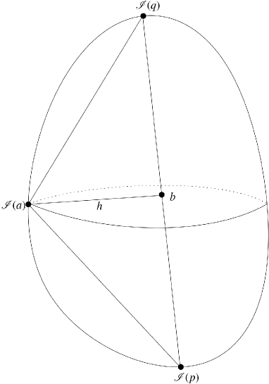
Figure 5. The Euclidean Triangle

∎

4. The almost rigidity for extrinsic diameter

From Remark 3.6, we know that $\mathscr{I}(M^{n})$ is in a small neighborhood of the line segment $\overline{\mathscr{I}(p)\mathscr{I}(q)}\subseteq\mathbb{R}^{m}$, where $\mathscr{I}\in\mathcal{IE}((M^{n},g),\mathbb{R}^{m})$ and $|\mathscr{I}(p)-\mathscr{I}(q)|$ is the extrinsic diameter of $\mathscr{I}(M^{n})$ in $\mathbb{R}^{m}$. In other words, the manifold $\mathscr{I}(M^{n})\subseteq\mathbb{R}^{m}$ is close to $\overline{\mathscr{I}(p)\mathscr{I}(q)}$ in $\mathbb{R}^{m}$.

However, to get the upper bound of the Gromov-Hausdorff distance between $\mathscr{I}(M^{n})$ and $\overline{\mathscr{I}(p)\mathscr{I}(q)}$, we also need suitable information about the second fundamental form $\mathscr{I}(M^{n})\subseteq\mathbb{R}^{m}$.

When the co-dimension of $\mathscr{I}(M^{n})$ is $1$, we get the positiveness of the second fundamental form for $\mathscr{I}(M^{n})\subseteq\mathbb{R}^{n+1}$ as follows.

Lemma 4.1.

If $(M^{n},g)\subset\mathbb{R}^{n+1}$ is a compact Riemannian manifold with $Rc(g)>0$, then $(M^{n},g)$ is a closed, strictly convex hypersurface in $\mathbb{R}^{n+1}$.

Proof.

Without loss of generality, we assume $\{\lambda_{i}\}_{i=1}^{n}$ are the principal curvatures of $(M^{n},g)\subset\mathbb{R}^{n+1}$ and $\lambda_{1}\leq\cdots\leq\lambda_{n}$. We firstly show that the principal curvature $\lambda_{i}(M^{n})>0$ for $i=1,\cdots,n$.

If $\lambda_{n}<0$ or $\lambda_{1}>0$, we are done.

Otherwise, there is $1\leq i_{0}\leq n$ such that

(4.1) $$\lambda_{i_{0}}\leq 0\leq\lambda_{i_{0}+1}.$$

From the Gauss equation on $(M^{n},g)\subseteq\mathbb{R}^{n+1}$, the Ricci curvature of $g$ is as follows:

(4.2) $$R_{i_{0}i_{0}}=\lambda_{i_{0}}(H-\lambda_{i_{0}})>0,$$

(4.3) $$R_{i_{0}+1,i_{0}+1}=\lambda_{i_{0}+1}(H-\lambda_{i_{0}+1})>0,$$

where $\displaystyle H=\sum_{i=1}^{n}\lambda_{i}$ is the mean curvature.

From (4.1) and (4.2), we get

(4.4) $$H-\lambda_{i_{0}}<0.$$

By (4.1) and (4.3), we have

(4.5) $$H-\lambda_{i_{0}+1}>0.$$

Now by (4.4) and (4.5), we obtain $\displaystyle\lambda_{i_{0}+1}<H<\lambda_{i_{0}}$. It is the contradiction.

The conclusion follows from that all $\lambda_{i}>0$ and [VH, Theorem, page $241$]. ∎

The following estimate for convex hypersurface is used to control the Gromov-Hausdorff distance in Theorem 4.4.

Lemma 4.2.

For $r>0$ and $n\geq 1$, if $\Sigma^{n}\subseteq B(r)\subseteq\mathbb{R}^{n+1}$ is a closed convex hypersurface, then

$$\mathcal{H}^{n}(\Sigma^{n})\leq\mathcal{H}^{n}(\partial B(r)),$$

where $\mathcal{H}^{n}$ is $n$-dimensional Hausdorff measure and $B(r)$ is the ball with radius $r$ in $\mathbb{R}^{n+1}$.

Proof: Let $\Omega$ be the convex set enclosed by $\Sigma^{n}$ with $\partial\Omega=\Sigma^{n}$. Define the map $\mathcal{P}:\overline{B(r)}\rightarrow\Omega$ as

$$d(x,\mathcal{P}(x))=\inf_{y\in\Omega}d(x,y),$$

which is a well-defined Lipschitz map with Lipschitz constant $\leq 1$(see [Brezis, Theorem $5.2$ and Proposition $5.3$]).

It is easy to get that $\mathcal{P}(\partial B(r))\subseteq\partial\Omega=\Sigma^{n}$. Now $\mathcal{H}^{n}(\Sigma^{n})\leq\mathcal{H}^{n}(\partial B(r))$ follows from the area formula for Lipschitz map $\mathcal{P}$ (see [EG]). ∎

Let $(X,d_{X})$ and $(Y,d_{Y})$ be two metric spaces, a map $F:X\rightarrow Y$ is called an $\epsilon$-Gromov-Hausdorff approximation if

$$Y\subset\mathbf{U}_{\epsilon}\Big{(}F\big{(}X\big{)}\Big{)},\quad\quad\sup_{x_{1},x_{2}\in X}\Big{|}d_{Y}\big{(}F(x_{1}),F(x_{2})\big{)}-d_{X}(x_{1},x_{2})\Big{|}\leq\epsilon.$$

The following lemma is closely related to [Gromov-book, $3.4(d_{+})$, Proposition $3.5$].

Lemma 4.3.

Let $(X,d_{X})$ and $(Y,d_{Y})$ be two metric spaces, if there is an $\epsilon$-Gromov-Hausdorff approximation $F:X\rightarrow Y$, then $\displaystyle d_{GH}(X,Y)\leq 4\epsilon$.

Proof: Step (1). We choose an $\epsilon$-dense net $\{x_{i}\}_{i\in I}$ of $X$, define $y_{i}=F(x_{i})\in Y$. Let $Z=X\sqcup Y$, define $d_{Z}\big{|}_{X}=d_{X},d_{Z}\big{|}_{Y}=d_{Y}$ and

$$d_{Z}(x,y)=\epsilon+\inf_{i}[d_{X}(x,x_{i})+d_{Y}(y,y_{i})],\quad\quad\forall x\in X,y\in Y.$$

We can verify that $(Z,d_{Z})$ is a metric space and $X,Y$ are isometrically embedded into $Z$.

Step (2). Note for any $y\in Y$, because $F$ is an $\epsilon$-Gromov-Hausdorff approximation from $X$ to $Y$, there is $x\in X$ such that

$$d_{Y}(y,F(x))\leq\epsilon.$$

Since $\{x_{i}\}$ is an $\epsilon$-dense net in $X$, there is $i_{0}\in I$ such that $d_{X}(x,x_{i_{0}})\leq\epsilon$. Then

$$d_{Z}(x_{i_{0}},y) \leq\epsilon+d_{X}(x_{i_{0}},x_{i_{0}})+d_{Y}(y,y_{i_{0}})=\epsilon+d_{Y}(y,F(x_{i_{0}}))$$

$$\leq\epsilon+d_{Y}(y,F(x))+d_{Y}(F(x),F(x_{i_{0}}))\leq 2\epsilon+d_{X}(x,x_{i_{0}})+\epsilon\leq 4\epsilon.$$

From the above, we obtain $Y\subseteq\mathbf{U}_{4\epsilon}(X)\subseteq Z$.

Step (3). On the other hand, for any $x\in X$, there is $x_{i_{0}}$ such that $d_{X}(x,x_{i_{0}})\leq\epsilon$.

Now we get

$$d_{Z}(x,y_{i_{0}})\leq\epsilon+d_{X}(x,x_{i_{0}})+d_{Y}(y_{i_{0}},y_{i_{0}})\leq 2\epsilon.$$

Therefore $X\subseteq\mathbf{U}_{2\epsilon}(Y)\subseteq Z$.

From the above and the definition of Gromov-Hausdorff distance, the conclusion follows. ∎

Now we are ready to prove the main theorem in this section.

Theorem 4.4.

For complete Riemannian manifold $(M^{n},g)$ with $K(g)\geq 1$ and $\displaystyle\mathcal{IE}((M^{n},g),\mathbb{R}^{n+1})\neq\emptyset$, we have

$$\frac{d_{GH}((M^{n},g),[0,\pi])}{\sqrt{\pi-\mathrm{Diam}_{\mathbb{R}^{n+1}}(M^{n},g)}}\leq 4\pi^{\frac{3}{2}}.$$

Proof: Step (1). We firstly choose a map $\mathscr{I}\in\mathcal{IE}((M^{n},g),\mathbb{R}^{n+1})$ freely. In the rest argument, we assume $\mathrm{Diam}_{\mathscr{I}}(M^{n},g)=|\mathscr{I}(p)-\mathscr{I}(q)|=\pi-\epsilon$ for some $p,q\in M^{n}$, where $\epsilon>0$. Assume $d_{g}(p,q)=\pi-\delta$, then $\delta\leq\epsilon$.

Without loss of generality, we assume that $\mathscr{I}(q)$ is the origin in $\mathbb{R}^{n+1}$, and $\frac{\mathscr{I}(p)-\mathscr{I}(q)}{|\mathscr{I}(p)-\mathscr{I}(q)|}$ is the positive direction of $x_{n+1}$-axis. Define the projection map $P:\mathbb{R}^{n+1}\rightarrow\mathbb{R}$, by $P(x_{1},\cdots,x_{n+1})=x_{n+1}$.

In the rest, we assume $t\in[0,\pi-\epsilon]$. Define $w_{t}\vcentcolon=l_{\mathscr{I}(p),\mathscr{I}(q)}\cap P^{-1}(t)$. For any point $c\in P^{-1}(t)\cap\mathscr{I}(M^{n})$, we have $l_{w_{t},c}\perp l_{\mathscr{I}(p),\mathscr{I}(q)}$. By Proposition 3.5, we know that $|w_{t}-c|\leq\sqrt{\pi\operatorname{\epsilon}}.$

So $(P^{-1}(t)\cap\mathscr{I}(M^{n}))\subset\Big{(}B_{w_{t}}(\sqrt{\pi\operatorname{\epsilon}})\cap P^{-1}(t)\Big{)},$ where $B_{w_{t}}(\sqrt{\pi\operatorname{\epsilon}})$ is the open ball in $\mathbb{R}^{n+1}$ centered at $w_{t}$ with the radius $\sqrt{\pi\operatorname{\epsilon}}$ (see Figure 6).

Figure 6. Cut $\mathscr{I}(M^{n})$ by $P^{-1}(t)$

From Lemma 4.1, we get that $\mathscr{I}(M^{n})$ is a strictly convex hypersurface in $\mathbb{R}^{n+1}$. For any distinct two points $y_{1},y_{2}\in P^{-1}(t)\cap\mathscr{I}(M^{n})$, consider the $2$-dim plane $\mathbf{P}$ determined by $w_{t},y_{1},y_{2}$, then $\gamma\vcentcolon=\mathbf{P}\cap\mathscr{I}(M^{n})$ is a closed convex curve in $\mathbf{P}=\mathbb{R}^{2}$ (see Figure 7).

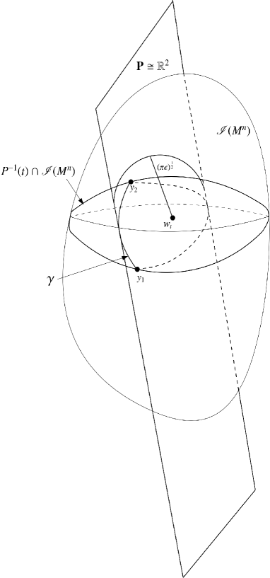
Figure 7. Cut $\mathscr{I}(M^{n})$ by $\mathbf{P}$

From the above, we get that

(4.6) $$\gamma\subseteq(\mathbf{P}\cap B_{w_{t}}(\sqrt{\pi\operatorname{\epsilon}})).$$

By Lemma 4.2 and (4.6), we have

$$d_{g}(\mathscr{I}^{-1}(y_{1}),\mathscr{I}^{-1}(y_{2}))\leq\frac{1}{2}\ell(\gamma)\leq\pi\sqrt{\pi\epsilon},\quad\quad\quad\forall y_{1}\neq y_{2}\in P^{-1}(t)\cap\mathscr{I}(M^{n}).$$

Therefore we obtain

(4.7) $$d_{g}(p_{1},p_{2})\leq\pi\sqrt{\pi\epsilon},\quad\quad\forall p_{1},p_{2}\in M^{n}\ \text{with}\ P(\mathscr{I}(p_{1}))=P(\mathscr{I}(p_{2})).$$

Step (2). Define $h:M^{n}\rightarrow\mathbb{R}$, by $h(z)=P(\mathscr{I}(z))$ for any point $z\in M$. Then the range of $h$ is $[0,\pi-\epsilon].$

Assume $\gamma_{q,p}$ is one unit speed, geodesic segment from $q$ to $p$ in $(M^{n},g)$. Define the map $G:[0,\pi]\rightarrow(M^{n},g)$ as follows:

$$G(t)=\left\{\begin{array}[]{rl}&\gamma_{q,p}(t-\frac{\delta}{2})\ ,\quad\quad\quad\quad\quad\quad t\in[\frac{\delta}{2},\pi-\frac{\delta}{2}],\\ &q,\quad\quad\quad\quad\quad\quad t\in[0,\frac{\delta}{2}],\\ &p,\quad\quad\quad\quad\quad\quad t\in[\pi-\frac{\delta}{2},\pi].\end{array}\right.$$

For $t_{1},t_{2}\in[0,\pi]$, note $\epsilon\leq\pi$, we have

$$\sup_{t_{1},t_{2}\in[0,\pi]}\Big{|}|t_{1}-t_{2}|-d_{g}(G(t_{1}),G(t_{2}))\Big{|}\leq\delta\leq\epsilon\leq\sqrt{\pi\epsilon}.$$

For any $y\in M^{n}$, we define $\varphi:M^{n}\rightarrow\mathbb{R}^{n+1}$ by requiring $\varphi(y)\in(\mathscr{I}(\gamma_{q,p})\cap P^{-1}(h(y)))\subseteq\mathbb{R}^{n+1}$ (note the choice of $\varphi$ is possibly not unique).

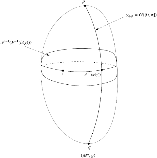
Figure 8. The $(\pi^{\frac{3}{2}}\cdot\sqrt{\epsilon})$-Gromov-Hausdorff approximation

Note $\mathscr{I}(y),\varphi(y)\in P^{-1}(h(y))$. By (4.7), we obtain

$$d_{g}(y,G[0,\pi])=d_{g}(y,\gamma_{q,p})\leq d_{g}(y,\mathscr{I}^{-1}(\varphi(y)))\leq\pi\sqrt{\pi\epsilon}.$$

Hence $G$ is an $(\pi^{\frac{3}{2}}\cdot\sqrt{\epsilon})$-Gromov-Hausdorff approximation from $[0,\pi]$ to $(M^{n},g)$ (See Figure 8).

By all the above and Lemma 4.3 , we get

$$d_{GH}((M^{n},g),[0,\pi])\leq 4\cdot\pi^{\frac{3}{2}}\cdot\sqrt{\pi-\mathrm{Diam}_{\mathscr{I}}(M^{n},g)}.$$

Because $\mathscr{I}$ is freely chosen from $\mathcal{IE}((M^{n},g),\mathbb{R}^{n+1})$, the conclusion follows.

∎