Testing the Fairness-Improvability of Algorithms
Abstract.
Many algorithms have a disparate impact in that their benefits or harms fall disproportionately on certain social groups. Addressing an algorithm’s disparate impact can be challenging, however, because it is not always clear whether there exists an alternative more-fair algorithm that does not compromise on other key objectives such as accuracy or profit. Establishing the improvability of algorithms with respect to multiple criteria is of both conceptual and practical interest: in many settings, disparate impact that would otherwise be prohibited under US federal law is permissible if it is necessary to achieve a legitimate business interest. The question is how a policy maker can formally substantiate, or refute, this “necessity” defense. In this paper, we provide an econometric framework for testing the hypothesis that it is possible to improve on the fairness of an algorithm without compromising on other pre-specified objectives. Our proposed test is simple to implement and can incorporate any exogenous constraint on the algorithm space. We establish the large-sample validity and consistency of our test, and demonstrate its use empirically by evaluating a healthcare algorithm originally considered by Obermeyer et al. (2019). In this demonstration, we find strong statistically-significant evidence that it is possible to reduce the algorithm’s disparate impact without compromising on the accuracy of its predictions.
1. Introduction
As algorithms are increasingly used to guide important predictions about people (e.g. which patients to treat, or which borrowers to grant a loan), substantial concern has emerged about their potential disparate impact—namely, that the algorithm’s benefits or harms may be born unequally across different social groups. Disparate impact has been empirically documented in a range of applications (see for instance Angwin and Larson, 2016; Obermeyer et al., 2019; Arnold et al., 2021; Fuster et al., 2021), but the organizations that deploy these algorithms also value other objectives such as accuracy and profit. When an algorithm has a disparate impact, is it possible to reduce that disparity without compromising the organization’s other objectives? The answer to this question is legally relevant. In many settings, a policy with a disparate impact that would otherwise be prohibited under US federal law is permissible if it is necessary to achieve a legitimate business interest (see Section 1.1 for a discussion). As a result, it is essential for both external regulators and internal stakeholders to have tools that can determine when fairness is in conflict with other objectives, and when instead there exist alternative algorithms that do better on all of the specified criteria. In this paper, we provide a framework and results for establishing, or refuting, the existence of such algorithms. We also suggest practical approaches for finding these algorithms when they exist.
Our paper consists of three parts. In the first part, we formally define fairness-improvability, along with an accompanying notion of accuracy-improvability (where we use “accuracy” as an umbrella term for any objective not directly related to inequities across groups). In the second part, we provide a procedure for testing fairness-improvability and accuracy-improvability of a status quo algorithm given data. Our proposed approach is simple to implement, flexible with respect to the definitions of fairness and accuracy, and can incorporate any exogenous constraint on the algorithm space. In the third part, we apply our procedure to show that a healthcare algorithm studied in Obermeyer et al. (2019) is both fairness- and accuracy-improvable.
To define fairness- and accuracy-improvability, we build on the framework of Liang et al. (2022). An algorithm is defined to be a mapping from a vector space of observed covariates (e.g. a medical profile) into a prediction (e.g. a medical diagnosis). There are two predefined groups. Algorithms are evaluated in terms of their accuracy for each group and their fairness across groups. Accuracy for each group is measured by a pre-specified utility function; for example, whether the algorithm makes an accurate diagnosis or whether a patient is treated. Fairness is measured using a potentially, but not necessarily, different utility function. We define an algorithm to be -fairness improvable if there is another algorithm that strictly improves on fairness by at least percent without any reduction in accuracy. Similarly, we define an algorithm to be -accuracy improvable if there is another algorithm that strictly improves on accuracy by at least percent without compromising fairness. In both cases, improvability is defined with respect to a fixed population distribution.
In practice the analyst may not know this distribution. We suppose that the analyst does however have access to a sample of individuals, their covariates, and a “ground truth” outcome (i.e., a quantity that determines the optimal algorithm and is known ex-post). The sample can be used to estimate and make inferences about the fairness and accuracy of the status quo algorithm in the population. The goal of our test procedure is to determine whether there exists another algorithm that improves on both criteria simultaneously.
Our test procedure is as follows. We first split the data into two subsets: a training set and a test set. We use the training set to identify a candidate algorithm that potentially improves on the status quo. Any method for identifying a candidate algorithm—which we call a selection rule—can be used here, subject to certain regularity conditions. We reference several possible selection rules from earlier work on algorithmic fairness (see Section 1.2 below). Once a candidate algorithm has been identified, we evaluate whether the improvements are statistically significant with the test set. We use the bootstrap to compute the critical values of our test. While our use of the bootstrap is standard, its justification is complicated by the fact that we impose very few restrictions on the selection rule. In particular, the distribution of our test statistic may vary with the sample size and is not guaranteed to “settle down” in the limit. To our knowledge, there does not exist a generally available bootstrap validity result that covers our exact setting. We thus prove a new bootstrap consistency result for our setting, building on a result for triangular arrays due to Mammen (1992): see Appendix B.1 for details.
To reduce the uncertainty introduced by sample-splitting, we recommend that the analyst repeats the above process several times and aggregates the results by reporting the median -value across the set of tests. We show that an asymptotically valid test is obtained by rejecting the null hypothesis whenever the median -value falls below half of the desired significance level. We further establish that this test is consistent under an additional assumption on the selection rule that we call improvement consistency. This condition says that whenever the status quo algorithm is indeed fairness-improvable (or accuracy-improvable), the selection rule will find it asymptotically.
Our proposed approach is designed to overcome a key practical challenge, which is that algorithms are often exogenously constrained for legal, logistical, or ethical reasons. The exact nature of these constraints may vary across settings, and include (among others) capacity constraints on how many individuals are admitted or treated, shape constraints such as monotonicity of the decision with respect to a given input (Wang and Gupta, 2020; Feelders, 2000; Liu et al., 2020), and statistical constraints such as requiring independence of decisions with a group identity variable (Mitchell et al., 2021; Barocas et al., 2023). Sample splitting and the bootstrap ensure that our test procedure is valid regardless of the specific class of algorithms, constraints, or utility functions chosen, subject to the regularity conditions given in Assumptions 1 and 2.
Finally, to illustrate our proposed procedure, we revisit the data and setting of Obermeyer et al. (2019). The status quo algorithm is one used by a hospital to identify patients for automatic enrollment into a high-intensity care management program. Using our framework and test procedure, we reject the null hypothesis that it is not possible to simultaneously improve on the accuracy and the fairness of the algorithm. We further quantify the extent of possible improvement by testing the null that the hospital’s algorithm is not -fairness improvable and -accuracy improvable for different values of . We find that large improvements in fairness are possible without compromising accuracy, while the reverse is not true.
1.1. Legal framework
The econometric framework we develop in this paper is broadly applicable whenever a policy maker wants to examine whether it is possible to increase the fairness of a policy without sacrificing other objectives. However, we think that our contribution should be particularly relevant to regulators and other legal decision makers tasked with evaluating cases of alleged disparate impact.
To support this application, we review the legal process for making a disparate impact case under US federal law.111We focus on restrictions of private individuals (as opposed to government agents) from certain policies. As a general rule, discrimination is legally permissible by private actors except when specifically prohibited by law. There is no singular discrimination law. However, there is a body of legislation, regulation, and court precedent that prohibits discrimination against certain social groups or protected classes such as those defined by race, gender, or religion in settings as varied as in employment, healthcare, education, and lending. US federal law generally distinguishes between two types of discrimination: disparate treatment and disparate impact. A policy has a disparate treatment if it intentionally offers different services based on an individual’s membership in a protected class. It has a disparate impact if one protected class is benefited or harmed more than another by the policy. Our paper pertains to disparate impact, which we broadly review here. Details and specific references to the US Code, the Code of Federal Regulations, and the Department of Justice’s Guidelines are deferred to Appendix D.
A typical process for evaluating a disparate impact case has three parts. The first part is to determine whether the benefits or harms disproportionately affect members of a protected class. This is often called a “prima facie” case of discrimination. For this part of the process, there already exist well-established statistical frameworks (see for instance Hazelwood School District v. United States, 1977; Shoben, 1978; Groves v. Alabama State Bd. of Educ., 1991), so we do not focus on it in our paper.
If the prima facie case is not successful, then the process ends and concludes that there is no disparate impact. If it is successful, then the second part of the process is to determine whether the challenged policy is a business necessity, i.e., necessary to achieve some legitimate nondiscriminatory interest. If the business necessity defense is not successful, then the process ends and concludes that the disparate impact is not permissible. If it is successful, then the third and final part of the process is to determine whether there exists a valid alternative that is less discriminatory, but still serves the same interests as the challenged policy. The policy is not permissible if such an alternative exists. Otherwise it is. Our econometric framework is relevant for this final part.
The exact implementation of this three-part process depends on the setting, and in particular on the specific statute, regulation, or court precedent prohibiting discrimination that is allegedly violated. For example, in the context of employment discrimination (which is prohibited by Title VII of the Civil Rights Act of 1964), either the Equal Employment Opportunity Commission or private individuals can bring a lawsuit in court to remedy a disparate impact violation. In this setting, the three-part test is adversarial; that is, there are two opposing parties, where one party is responsible for the evidence and arguments supporting the policy, and the other party is responsible for the evidence and arguments against the policy. In contrast, in the context of discrimination by a program or activity that receives federal funding (which is prohibited by Title VI of the Civil Rights Act of 1964), investigation and enforcement instead falls on the funding agency (see Alexander v. Sandoval, 2001). Though the funding agency’s determination of disparate impact is not typically viewed as adversarial, the Department of Justice still recommends using the three-part test outlined above.222The Department of Justice is tasked with coordinating the implementation and enforcement of Title VI across federal agencies, by Executive Order 12250, 28 C.F.R. pt. 41, app. A. Their guidelines can be found in the Title VI Legal Manual available at https://www.justice.gov/crt/fcs/T6manual.
Twenty-six funding agencies currently enforce Title VI in a variety of contexts such as education, healthcare, and transportation. In Section 5, we apply our framework to study a potential disparate impact in access to hospital services. If the hospital receives federal funding from Medicare or Titles VI or XVI of the Public Health Service Act, this discrimination would be prohibited by Title VI of the Civil Rights Act of 1964. In this case, a likely enforcing agency would be the US Department of Health and Human Services (HHS).333Specific referrals of individual complaints to HHS can be found at https://www.hhs.gov/civil-rights/for-individuals/index.html and https://www.cms.gov/about-cms/web-policies-important-links/accessibility-nondiscrimination-disabilities-notice. As hospitals and other healthcare providers increasingly use algorithms to allocate resources and determine patient care, we view our framework as one that could potentially be used by HHS in order to evaluate allegations of discrimination under Title VI.
1.2. Related Literature
Our paper is related to several literatures in economics, statistics and computer science which study algorithmic fairness: see Chouldechova and Roth (2018), Cowgill and Tucker (2020), or Barocas et al. (2023) for recent overviews. Most of this literature is concerned with computational and algorithmic aspects of fair algorithm design. For example, many papers build an explicit fairness constraint into the optimization problem, and focus on the question of how to find (or approximate) the optimum in a computationally efficient manner (Dwork et al., 2012; Agarwal et al., 2018; Kusner et al., 2019; Dwork et al., 2018; Babii et al., 2020; Viviano and Bradic, 2023). Coston et al. (2021) share our motivation of evaluating whether an algorithm with disparate impact can be justified by business necessity, and formulate an optimization problem in which disparate impact is minimized over a set of algorithms that satisfy an additional constraint.
We focus on the different but complementary problem of statistical inference, and develop an econometric framework to test whether there exists an algorithm that satisfies the same business objectives but has lower disparate impact. We abstract away from the question of how to efficiently search for a fairness-improving algorithm; any of the methods developed in this literature could be used within our proposed procedure as a means to identify candidate algorithms for fairness-improvement.
Our sample-splitting procedure is closely related to that proposed in Blattner and Spiess (2023), which studies potential fairness and intepretability improvements in lending algorithms. Although the mechanics of our two procedures are different, we both use training data to identify a “less discriminatory algorithm” and test data to evaluate it. Relative to this work, our paper contributes formal statistical guarantees.
Another closely related paper is the work of Liu and Molinari (2024), which directly estimates the fairness-accuracy frontier developed by Liang et al. (2022). A full characterization of the frontier allows the analyst to answer a broad range of questions related to algorithmic fairness. In particular, once the fairness-accuracy frontier has been characterized, testing for the fairness-improvability of a status-quo algorithm amounts to testing whether or not the algorithm belongs to the frontier. While our approach focuses on the narrower question of testing for fairness-improvability (rather than characterizing the full frontier), it is more flexible in two ways—(1) we can accommodate definitions of accuracy and fairness with respect to different utility functions, and (2) we can accommodate (almost) any exogenous constraint on the algorithm space.444The characterization of the frontier in Liu and Molinari (2024) is developed for the class of all possible algorithms, and (to the best of our knowledge) extends under specific restrictions on the algorithm space, which rule out global constraints such as capacity constraints and monotonicity constraints. We view these features as enhancing the practical utility of our proposed method.
2. Model
2.1. Setup
Consider a population of individuals, where each individual is described by a covariate vector taking values in the set , a type taking values in , and a group identity taking values in . The covariates in are the information that the algorithm can access to make a decision, the type is a payoff-relevant unknown that the algorithm cannot directly access, and the group identity is a special covariate (which the algorithm may or may not access555The algorithm is given only as input, but we allow for the possibility that is a covariate in , or is perfectly correlated with covariates in .) which is used to evaluate the fairness of the algorithm.
We use to denote the joint distribution of across individuals. The analyst does not know this distribution, but observes a sample consisting of independent and identically distributed observations from . An algorithm maps covariate vectors into a decision in . Throughout we use to denote the decision taken by the algorithm.
We evaluate algorithms from the perspectives of accuracy and fairness, which are defined with respect to an accuracy utility function , and a (possibly identical) fairness utility function . We will consider accuracy and fairness criteria that can be formulated as
| (2.1) |
where and are normalization functions (see Examples 1-4 for possible specifications). Thus, and are normalized expected utilities for each group according to the respective utility functions. When the utility functions and normalization functions are common across accuracy and fairness, we drop the subscripts and write .
We say that one algorithm is more accurate than another if the value of is larger for both groups, and more fair if the value of differs less across groups.
Definition 2.1.
Algorithm is more accurate than algorithm if
and more fair than algorithm if
We list below some example utility specifications from the prior literature.666Examples 1-3 are popular in the algorithmic fairness literature (see e.g. Mitchell et al. (2021)), while Example 4 is a canonical example in economics. We drop the fairness and accuracy subscripts to simplify the exposition, understanding that the designer could use different utility specifications for accuracy and fairness.
Example 1 (Classification Rate).
The decision is a prediction of , and both are binary. Let be an indicator variable for whether the prediction is correct, and let the normalization function be . Then
is the correct classification rate of algorithm within group , while is the disparity in clasification rates across groups.
Example 2 (Calibration).
The type takes values in and the decision is binary. Define and . Then
is the expected type for individuals receiving decision in group , while evaluates how different these conditional expectations are across groups.
Example 3 (False Positive Rate).
Let . Define and . Then
is the probability of choosing the (wrong) decision for individuals with true type in group , while compares the probability of this error across groups.
Example 4 (Profit).
There is a good that is offerred to an individual at price . The individual’s unknown willingness-to-pay is . The utility function is
and the normalization function is . That is, the firm receives the price if the individual’s willingness to pay exceeds that price, and otherwise the firm receives nothing. Then is the profit the firm receives from group consumers, and is the difference in profit received from consumers of either group.
In some applications, the analyst may wish to consider an accuracy measure that is unconditional across groups (e.g., the expected utility in the entire population), or to require simultaneous fairness improvements according to several different utility functions.777For example, the analyst may require a fairness improvement not only with respect to the utility function given in Example 2, but also with respect to the mirrored utility function that conditions on . Indeed, the property popularly known as calibration requires improvements according to both of these measures (Chouldechova, 2017; Kleinberg et al., 2017). Our procedure and results can be straightforwardly extended in either of these cases, but we will present our results for the three criteria , , and proposed here.
For a fixed class of algorithms , the feasible accuracy and unfairness levels are those triples that can be achieved by some algorithm in . Our proposed testing procedure will be agnostic about the specific choice of , and in particular we will allow for to be exogenously restricted in some way. We view this flexibility as important since (as discussed in the introduction) in practice there are often legal, logistical, or ethical constraints on which algorithms can be implemented.
2.2. Accuracy/Fairness Improvability
There is a status quo algorithm representing an algorithm that is already in use, or which has been proposed for use. The status quo algorithm has some level of fairness, , and we want to know whether it is possible to improve upon this without compromising on accuracy.
Definition 2.2 (Accuracy-Fairness Improvement).
Fix any . The algorithm constitutes a -improvement on the algorithm if
That is, algorithm constitutes a -improvement on algorithm if it leads to a -percent increase in accuracy for group , a -percent improvement in accuracy for group , and a -percent reduction in disparate impact.
Definition 2.3 (Fairness Improvability).
Fix a class of algorithms and any . The algorithm is -fairness improvable within class if there exists an algorithm that -improves on , i.e.,
If an algorithm is -fairness improvable, then it is possible for the firm to strictly improve on fairness by at least percent without compromising on accuracy. We view this definition as directly related to the business-necessity defense in a disparate impact case (as described in Section 1.1). When captures a business-relevant objective, then -fairness improvability corresponds to the existence of an alternative algorithm that can achieve the same business objectives with less disparate impact. In the special case where , the disparate impact of algorithms that are not -fairness improvable are necessary to achieve the business objective.
A complement to the above condition is the following pair of definitions:
Definition 2.4 (Accuracy Improvability).
Fix a class of algorithms and any .
-
(a)
The algorithm is -accuracy improvable for group within class if there exists an algorithm that -improves on , i.e.,
where .
-
(b)
The algorithm is -jointly accuracy improvable within class if there exists an algorithm that -improves on , i.e.,
That is, an algorithm is -accuracy improvable for group if it is possible to improve accuracy for group by at least without compromising on accuracy for the other group or on fairness. The algorithm is -jointly accuracy improvable if it is possible to improve accuracy for both groups by at least without compromising on fairness.
In the special case in which , then all of these definitions coincide, and correspond to a simultaneous strict improvement in accuracy for both groups as well as in fairness. When this holds we say that algorithm is strictly FA-dominated within class .
3. Proposed Approach
We now propose a procedure for testing fairness-improvability and accuracy-improvability of a status quo algorithm . The analyst specifies a set of algorithms and we consider testing the null hypothesis
| (3.1) |
against the alternative that such an improvement exists. Section 3.1 outlines the approach, and Sections 3.2 and 4 establish the validity of our procedure.
3.1. Description of Procedure
The analyst first chooses a selection rule that maps samples into a choice of algorithm from , i.e., a mapping
where is the set of all finite samples of observations. Our results apply for any such rule.
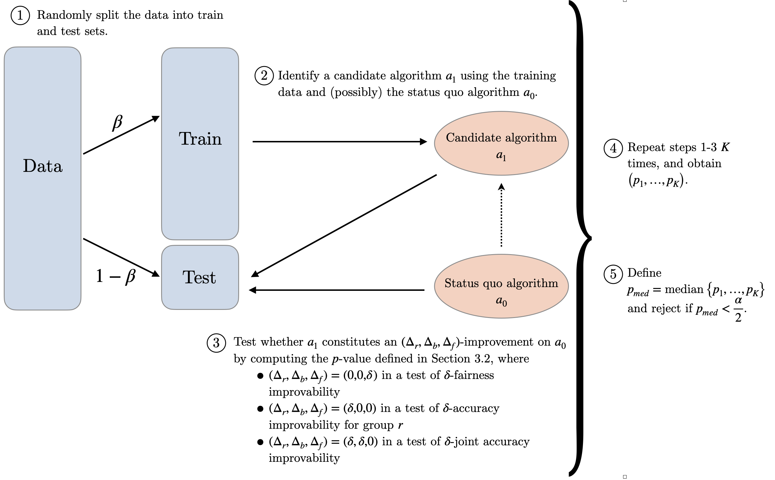
In each round of the procedure (where is chosen by the user), the analyst repeats the following steps:
[1] Split the sample into train and test. The training sample includes observations selected uniformly at random from , where is a user-chosen fraction (we use in our application). The test sample consists of the remaining observations.
[2] Find a candidate algorithm using the training sample. Apply the selection rule to the training sample . To simplify notation, we use to denote the (realized) algorithm , which serves as a candidate algorithm in the subsequent step.
[3] Test whether constitutes a -improvement relative to . Given the status quo algorithm and the candidate algorithm obtained in the previous step, test the null hypothesis
| (3.2) |
using the test outlined in Section 3.2. We set in a test of -fairness improvability, in a test of -accuracy improvability for group , and in a test of -joint accuracy improvability. Let denote the -value associated with this test (details below in Section 3.2).
The iterations of (a)-(c) yields a vector of -values . Define to be the median of the values and reject if and only if . Corollary 4.1 guarantees that this test is of level . This proposed procedure is summarized in Figure 1.
3.2. Testing whether constitutes a -improvement on .
This section provides supporting details and results for step [3] of our procedure.
Given fixed algorithms and , and test sample where , we consider testing the null hypothesis
| (3.3) |
against the alternative
for an arbitrary vector , where
denotes the accuracy and fairness levels under the status quo algorithm and
denotes the accuracy and fairness levels under the candidate algorithm . The choice of corresponds to a test of -fairness improvability, while the choice of corresponds to a test of -accuracy improvability for group .
Since is formulated as a union of three conditions, a test of can be constructed by first constructing tests for each of the conditions individually, and then combining the individual tests using the intersection-union method.888See Casella and Berger (2021) for a textbook reference on the intersection-union method. Proposition B.1 in the appendix develops straightforward modifications of Theorems 8.3.23-24 in Casella and Berger (2021) to an asymptotic setting. Specifically, we will construct tests for each of the individual conditions that make up , and reject if all three tests reject at once.
First, we specify test statistics for each of the individual tests that make up . To simplify the derivations, we introduce a slight change in notation. Let and define
where
and collects all of the unknown nuisance parameters which appear as normalizations in the utility specifications. This re-writing allows for the accuracy and fairness criteria and to be expressed as unconditional expectations of the functions , rather than as ratios of the conditional expectations of , , , (as defined in (2.1)). That is, and .
In the results that follow, we will in fact allow and to depend on the nuisance parameter more generally than what is considered above (see specifically Assumption 1). Since is unknown, it will need to be estimated in a first-stage when estimating the utility of a given algorithm. In general, we assume that can be written as where for some known function . For instance, consider the following example based on the calibration utility defined in Example 2.
Example 5.
Suppose we wish to test the null hypothesis in a setting where , and is given by the calibration utility defined in Example 2. Then is given by
where and
We estimate , , and using their empirical analogs , and . Our test statistics for the individual tests are then defined as follows. When testing whether is less accurate than for groups and , let
where for . When testing whether is less fair than , define
where
and
Given that we establish the asymptotic normality of our test statistics in Propositions B.2 and B.3 of the appendix, we could in principle use the quantiles of a standard normal distribution to construct critical values given consistent estimators of their asymptotic variances. However, under this approach, the appropriate estimators would need to be computed case-by-case for each utility function. Thus, we instead propose using the nonparametric bootstrap to generate the critical values. Specifically, if we fix at some nominal level, then for the accuracy parts of the test, the rejection rule is given by for , where is the quantile of the bootstrap distribution defined in the appendix. For the fairness part of the test, the rejection rule is given by where is the quantile of the bootstrap distribution defined in the appendix.
Our ultimate test of the null hypothesis (3.3) is then given by , i.e., we reject if and only if all three component tests reject.
4. Main Results
We now show that the test proposed in Section 3 is asymptotically valid when the candidate algorithm is selected using the data in . We will also show that the test is consistent under an additional assumption on the selection rule which we call improvement consistency.
First consider , i.e., there is only one round of sample-splitting. Let denote the realized split of training and testing samples of the data . Denote the candidate algorithm selected using rule on the training sample as
Consider using the test statistic (as defined in Section 3.2) to test the null hypothesis (3.3) on the test sample .
We first establish the asymptotic validity of the test under the following regularity conditions restricting the distribution and class of algorithms :
Assumption 1.
The nuisance parameters belong to an open convex subset . The functions and are twice continuously differentiable on for every , , and . Furthermore, is bounded, and , , and their first and second-order partial derivatives (with respect to ) are all uniformly bounded over .
Assumption 2.
The status quo algorithm is not perfectly fair, i.e. . Moreover, let denote the set of covariance matrices of the nuisance parameters and utilities (as defined in (B.3) in the appendix) for every candidate algorithm . Then we assume
for some , where denotes the smallest eigenvalue of .
Assumption 1 allows us to appropriately linearize the utility functions as a function of , uniformly over the parameter space . The uniformity of the linearization is important since the true value of the nuisance parameter can fluctuate as a function of sample size. The boundedness conditions in Assumption 1 impose implicit constraints on the parameter space and the support of the data. For instance, revisiting Example 5, we see that the support of should be bounded, and each component of should be bounded away from zero. Assumption 2 ensures that the limiting variances of our test statistics are non-degenerate uniformly in the space of candidate algorithms . Once again this uniform non-degeneracy is important since the candidate algorithm is allowed to vary arbitrarily as a function of sample size. Low level conditions which guarantee Assumption 2 are difficult to articulate at this level of generality, but intuitively, Assumption 2 requires that the variances of the utilities be bounded away from zero uniformly in the space of candidate algorithms, and that the correlation in the utilities between the status-quo and candidate algorithms be bounded away from one.
Theorem 4.1 establishes that the test is asymptotically of level regardless of the choice of algorithms , as long as the nuisance parameters and utilities are well-behaved over the the class as described in Assumptions 1 and 2.
Theorem 4.1.
In practice, a researcher may prefer to combine the test results over multiple splits of the data to reduce the unpredictability in the procedure induced by sample splitting. Formally, consider and let denote the realized split of training and testing samples in the -th round of sample splitting. Further let
denote the candidate algorithm selected using rule on the training sample . Define the test statistic to reject if the median test statistic (across the rounds of sample splitting) rejects. We establish the following corollary of Theorem 4.1:
Corollary 4.1.
Under the assumptions of Theorem 4.1,
Note that, as a consequence of Corollary 4.1, to ensure that the test is asymptotically of level we require that the component tests for are of level . Equivalently, we reject the null if the median -value (across the rounds of sample splitting) satisfies . We would in general expect this conservativeness to result in a loss of power relative to a test performed using a single split, but the local power analysis conducted in DiCiccio et al. (2020) suggests that this is not always the case. For example, their Theorem 3.1 shows that there is no loss in power for testing a mean when the alternative is not too close to the null.
Finally, we establish the consistency of the test under high-level conditions on the behavior of the selection rule .
Assumption 3.
Suppose the null hypothesis given in (3.1) does not hold. We say that the selection rule is improvement-consistent if, for , and for some algorithm that constitutes a -fairness (or accuracy) improvement over the algorithm .
In words, improvement consistency says that whenever there exists a fairness (or accuracy) improvement on the algorithm in , the selection rule is guaranteed to find it asymptotically. Theorem 4.2 establishes that the test is consistent (that is, has power approaching one for any distribution in the set of alternatives) if the selection rule is improvement consistent.
Theorem 4.2.
We expect that for many datasets, it will be possible to reject the null using a naive selection rule that does not satisfy improvement consistency, as is the case in our empirical illustration in Section 5. However, Theorem 4.2 guarantees that the null will be asymptotically rejected (in cases where it should be) when the selection rule satisfies this property. In Appendix C we propose selection rules (constructed using mixed integer linear programs) for certain common utility specifications, which we conjecture are improvement consistent.
5. Empirical Application
We illustrate our approach in the setting of Obermeyer et al. (2019). The status quo algorithm is a commercial healthcare algorithm used by a large academic hospital to identify patients to target for a high-risk care management program. The algorithm assigns to each patient a risk score, and identifies those with risk scores above the 97th percentile for automatic enrollment in the program. We use our proposed approach to evaluate the improvability of the hospital’s algorithm, finding that the hospital’s algorithm is strictly FA-dominated within the class of linear classifiers. That is, it is possible to simultaneously strictly improve on the accuracy and the fairness of the algorithm. We further quantify the extent of possible improvement by testing the null that the hospital’s algorithm is not -fairness improvable and -accuracy improvable for different values of . We find that large improvements in fairness are possible without compromising on accuracy, while the reverse is not true.
5.1. Data and Classification Problem
The data includes observations from 48,784 patients, among which 43,202 self-report as White and 5,582 self-report as Black. Following Obermeyer et al. (2019), we take these to be the two group identities, denoted . Each patient ’s covariate vector includes 8 demographic variables (e.g., age and gender), 34 comorbidity variables (indicators of specific chronic illnesses), 13 cost variables (claimed cost broken down by type of cost), and 94 biomarker and medication variables. Although group identity is known for each patient in the dataset, the status quo algorithm omits this variable for prediction, so we do as well. Finally, the data set reports each patient ’s total number of active chronic illnesses in the subsequent year, which is interpreted as a measure of the patient’s true health needs. We take this to be the patient’s type .
An algorithm assigns to each patient a decision based on the covariate vector , where 1 corresponds to an automatic enrollment into the care management program. We respect the capacity constraint of the status quo algorithm by restricting to algorithms that select 3% of the population for automatic enrollment.
Following Obermeyer et al. (2019), we evaluate both accuracy and fairness using the calibration utility function introduced in Example 2, i.e.
| (5.1) |
and
That is, an algorithm is more accurate if the expected number of health conditions is higher among both Black and White patients assigned to the program. It is more fair if it reduces the disparity in the expected number of health conditions among Black and White patients assigned to the program.999Here and throughout we drop the notational distinction between and , as they are identical in this example.
5.2. Results
We implement our proposed approach in Section 3 to test the fairness- and accuracy- improvability of the hospital’s algorithm. We use iterations and select a fraction of the data to use for training. The status quo algorithm assigns each patient a risk score, and chooses those patients with risk scores in the top 3% for automatic enrollment. Our candidate algorithms similarly assign risk scores to patients, and enroll those patients with the highest risk scores, but use different risk score assignments compared to the status quo algorithm.
Specifically, to identify candidate algorithms, we first use the training data to compute an alternative risk score assignment rule , which maps each covariate vector into a predicted number of health conditions. Then we use the trained prediction rule to rank all patients in the test data, and select the top 3% for automatic enrollment ().101010Obermeyer et al. (2019) find that the hospital’s algorithm was instead trained to predict a different outcome variable, namely health costs.
We consider several different methods for selecting a function —specifically, we choose to be the output of a linear regression, a lasso regression, or a random forest algorithm—but find that all of these yield similar results.111111The regularization parameter for LASSO is determined using 5-fold cross-validation. For random forest, we utilize a configuration of 300 trees with other hyperparameters set to their default values as specified in scikit-learn version 1.4.1. Figure 2 plots the average value (across the iterations of our procedure) of the utilities and under the status quo algorithm, as well as the average values for these utilities given candidate algorithms identified by each of the three methods mentioned above. This figure is suggestive that the candidate algorithms succeed in improving not only accuracy (each of and increase) but also fairness ( decreases).
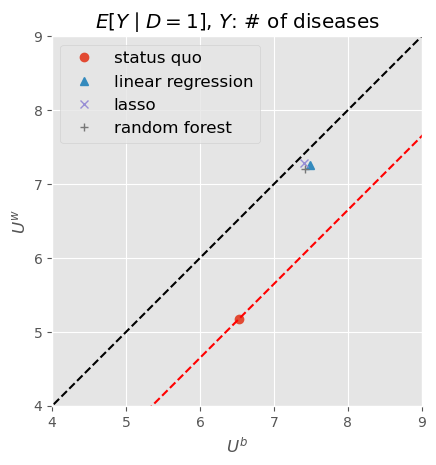
We subsequently report findings for the linear regression model only, deferring the (nearly identical) results for the other models to Appendix E. Table 1 complements Figure 2 by reporting the -values that emerge from our statistical test of the null hypothesis that the status quo algorithm is not strictly FA-dominated. Across the iterations of our procedure, the median -value is ; thus, we reject the null at the 10% significance level (recall that we reject at a significance level if the median -value is less than ). This means that, were the hospital to defend the disparate impact of its algorithm on account of necessity for a certain level of accuracy (as defined in (5.1)), a court could reject this business necessity claim with strong statistical guarantees.121212Our finding complements Obermeyer et al. (2019)’s result that training an algorithm to predict health needs (instead of health costs) leads to a more equal proportion of Black and White patients among those who are identified for automatic enrollment, without compromising accuracy. In each iteration of our procedure, the largest -value among , , and (i.e., the individual tests for accuracy improvement for each group and for fairness improvement defined in Section 3.2) is . Thus it is the fairness-improvement dimension in this problem that is binding.
| Accuracy (Black) | Accuracy (White) | Unfairness | ||||||||
|---|---|---|---|---|---|---|---|---|---|---|
| Iteration 1 | 7.27 | 6.33 | 0.0000 | 7.24 | 5.15 | 0.0000 | 0.28 | 1.17 | 0.0524 | 0.0524 |
| Iteration 2 | 7.37 | 6.37 | 0.0001 | 7.22 | 5.14 | 0.0000 | 0.15 | 1.23 | 0.0530 | 0.0530 |
| Iteration 3 | 7.70 | 6.67 | 0.0000 | 7.24 | 5.17 | 0.0000 | 0.47 | 1.50 | 0.0223 | 0.0223 |
| Iteration 4 | 7.42 | 6.38 | 0.0000 | 7.29 | 5.13 | 0.0000 | 0.13 | 1.25 | 0.0312 | 0.0312 |
| Iteration 5 | 7.65 | 6.88 | 0.0017 | 7.32 | 5.28 | 0.0000 | 0.33 | 1.60 | 0.0158 | 0.0158 |
We further explore the tradeoff between improvements in accuracy and fairness by subsequently testing for -fairness improvability, where we allow to vary. That is, we ask whether it is possible to improve on fairness by at least percent without compromising on accuracy. We find that we can reject the null at the 10% significance level for all . This means that even under an extremely stringent notion of what it means to improve on disparate impact—namely, that the status quo algorithm’s disparate impact is justified unless it is possible to reduce disparate impact by without compromising accuracy—the court would still be able to conclude that improvements are feasible. (For larger , it is possible that further reductions are also possible, but the data and/or our method of searching for a candidate algorithm do not allow us to conclude that such an improvement exists.)
We also test -accuracy improvability. Although it is not directly relevant for the legal framework described in Section 1.1, it does provide a complementary angle on the fairness-accuracy tradeoffs in this application. We find that we can only conclude that joint improvements in accuracy of up to 4.6% are possible. We subsequently separately test for -accuracy improvability for either group, and find that the binding dimension is accuracy improvement for Black patients. That is, while large gains in accuracy—up to 33.7%—can be achieved for White patients (without compromising accuracy for Black patients or fairness), we cannot conclude the same for Black patients. These findings are summarized in Table 2.
| largest | |
|---|---|
| -fairness improvable | 0.725 |
| -jointly accuracy improvable | 0.046 |
| -accuracy improvable for Black patients | 0.046 |
| -accuracy improvable for White patients | 0.337 |
The asymmetry between the extent of accuracy improvability for White patients and Black patients has two different explanations. One possibility is that large improvements in accuracy for Black patients necessarily conflict with one of the two other criteria (i.e., it implies either a reduction in accuracy for White patients or a reduction of fairness), while large improvements in accuracy for White patients can be achieved without sacrificing these other goals. Alternatively, it could be that the candidate algorithm simply does not substantially improve accuracy for Black patients.131313This could be, for example, because the measured covariates are not very predictive for this group. Our findings in Table 2 are explained by the latter: At the threshold value of where the median -value equals 0.05 (and we lose statistical significance), the binding -value in the joint test is the one corresponding to a -increase in accuracy for Black patients.
This is not a property of the data, but rather of our analysis in Table 2. Since we fix the selection of candidate algorithms in this analysis, the only value that varies with in our evaluation of -accuracy improvability for Black patients is the -value pertaining to accuracy for Black patients. (A similar statement holds for our other analyses in Table 2.) To evaluate the inherent conflicts in accuracy and fairness more directly, one might instead allow the choice of candidate algorithm to depend on , in which case all three -values in our joint test would vary with . We leave such explorations to future work.
6. Conclusion
When a commercial algorithm exhibits disparate impact, it can be important to understand whether it is possible to reduce that disparate impact without compromising on other business-relevant criteria, or if this level of disparate impact is necessitated by those other goals. We have designed a statistical approach to assess this, with three practical objectives in mind. First, since the appropriate definitions of disparate impact and business-relevant criteria vary substantially across applications, we want our framework to be flexible enough to accommodate any such definitions that may emerge in practice. Second, since there are often exogenous constraints on the algorithm space, we want our procedure to apply universally across algorithm classes. Finally, we would like for the approach to be transparent and simple to use for practitioners. The statistical framework that we propose delivers on these three counts.
The main drawback of our approach is its dependence on the selection rule for choosing a candidate algorithm. When we are able to reject the null, as in our application, then the optimality properties of the selection rule (in particular, whether it satisfies improvement consistency as defined in Section 4) do not matter. That is, no matter how naive or heuristic our selection rule is, we can conclude that the status quo algorithm is improvable. But when our test does not allow us to reject the null, there is in general an ambiguity: It may be that there is not sufficient evidence in the data to conclude existence of an improving algorithm; or, alternatively, it may be that the selection rule is not powerful enough to find this algorithm. In the latter case, re-running the same test with a different selection rule could lead us to reject the null. This ambiguity is resolved asymptotically when the selection rule is improvement consistent, since Theorem 4.2 establishes that our proposed test is consistent under this condition. An important direction for future work is thus to provide sufficient conditions for a selection rule to be improvement consistent in different relevant applications.
Appendix A Bootstrap algorithm
Let be the empirical distribution of the data and let denote a bootstrap sample drawn i.i.d from . Let , , denote the bootstrap analogs of , , computed using the bootstrap data. The bootstrap analogs of the test-statistics are given by
The critical values for the test are based on the quantiles of the bootstrap distribution of the test statistics. Specifically, let be the (conditional) cumulative distribution function of given and be the (conditional) cumulative distribution function of given . Of course, in practice these are not known exactly, but can be approximated via Monte-Carlo by taking independent bootstrap samples from and computing the empirical distribution
for , where denotes the bootstrap test statistic computed on the th sample.
Appendix B Proof of Main Results
Proposition B.1.
Let denote a set of distributions for which . Let denote the subset of distributions for which holds. Let , , be tests of the component null hypotheses for accuracy and fairness as defined in Section 3.2. Let for denote the subsets of distributions for which each holds. Define the test which rejects if and only if each test rejects for .
-
(1)
If for are asymptotically of level , i.e. if
for every , then is asymptotically of level , i.e.
for every .
-
(2)
If for are uniformly asymptotically of level , i.e. if
then is uniformly asymptotically of level , i.e.
Moreover, if there exists some distribution such that for some , and for , then
Proof.
To prove the first claim, note that by the definition of , for any ,
for every . By the definition of , for some . Since is asymptotically of level , it follows that
as desired.
To prove the second claim, first note that by following the argument above, for each we obtain
for some . It thus follows that
Since each is uniformly asymptotically of level , we then obtain that
| (B.1) |
Next, note that from the definition of ,
It thus follows by our assumptions on that
| (B.2) |
Combining (B.1) and (B.2) we thus obtain that
as desired. ∎
B.1. Bootstrap consistency
To demonstrate Theorems 4.1 and 4.2, we first show that the bootstrap procedure defined in Appendix B.1 is consistent when the test statistics are applied to an arbitrary deterministic sequence of candidate algorithms , i.e. that
as , for , where denotes the Kolmogorov metric and denotes the distribution function of a random variable . Note here that we have been careful to index each term in the expression by the total sample size , since in principle each of these objects could vary with the candidate algorithm , but we suppress for the rest of Section B.1 whenever we think it would not lead to confusion.
We prove bootstrap consistency in three steps. In the first step (Proposition B.2), we show that the asymptotic linear representations of the test statistics are asymptotically normal. In the second step (Proposition B,4), we demonstrate consistency of the bootstrap distribution for the asymptotic linear representations by invoking Theorem 1 of Mammen (1992). Finally in the third step we show that the bootstrap remains consistent when we move from the asymptotic linear representations to the original test statistics (Proposition B.3). Throughout this section we maintain Assumptions 1 and 2.
B.1.1. Asymptotic normality of the test statistic
We first write the test statistics as sample averages. To do this, we define
| (B.3) |
and
where refers to a dimensional vector of 0s. We also define
and
To demonstrate asymptotic normality of the test statistics, we derive their asymptotic linear representations. To do this, we use the additional definitions
where we note that these are dimensional vectors, and
Using these additional constructions, we can define the asymptotic linear representations of the test statistics and demonstrate their asymptotic normality. They are
First, we argue that the asymptotic linear representations are asymptotically normal.
Proposition B.2.
For ,
and
where and for , and is the Kolmogorov metric.
Proof.
For
Since is independent across the Lindeberg-Feller CLT implies that
where . Note that by Assumption 2. It thus follows by Polya’s Theorem (Theorem 11.2.9 in Lehmann and Romano, 2022) that
Similarly,
and
where . Note also that by Assumption 2. ∎
Second, we argue that the difference between the test statistics and their asymptotic linear representation are asymptotically negligible.
Proposition B.3.
For ,
Proof.
The result for the accuracy test statistics follows from
where the last equality is because .
The second equality follows from a Taylor expansion, Assumption 1, and the fact that by a standard concentration argument (e.g. Markov’s inequality). The third equality follows from a law of large numbers, , and some additional algebra.
The result for the fairness test statistic follows from
where is a dimensional identity matrix and is a dimensional matrix of s. The second equality is because and the third equality is because . They both follow from Assumption 1 and a standard concentration argument.
The second-to-last equation is because
where
for and so
∎
B.1.2. Asymptotic normality of the bootstrap distribution
Let the (infeasible) bootstrap distributions of and be denoted by and . We say that these distributions are infeasible because they depend on unknown population parameters.
Proposition B.4.
and .
Proposition B.5.
For ,
as .
Proof.
Let denote the bootstrap distribution of the data. By applying the logic of Proposition B.3 to the bootstrap data, it follows that
where . To establish our result, we argue along subsequences. To that end, for every subsequence there exists a further subsequence (which we index by ) such that
where the second convergence statement follows from Proposition B.3, the third from Proposition B.4, and the last convergence statement follows from Assumption 2. We thus have that
with probability one. It follows by Polya’s Theorem (Theorem 11.2.9 in Lehmann and Romano, 2022) that
and thus by Propositions B.2 and B.3,
Since we have established that for every subsequence there exists a further subsequence along which the convergence holds almost surely, the original sequence converges in probability, as desired. ∎
B.2. Proof of Theorem 4.1
Proof.
For an arbitrary deterministic sequence of algorithms , we want to show that for satisfying the null hypothesis,
By Proposition B.1 (1) it suffices to check that each test is asymptotically of level . We prove the result for the fairness test since the other results follow from the same logic. By definition,
since under the null hypothesis.
By Proposition B.5, for any and sufficiently large,
so that by Lemma A.1. (vii) in Romano and Shaikh (2012), we have that or sufficiently large
It thus follows that for sufficiently large,
from which we can conclude that
Next we argue that the result holds for the random sequence . By the law of iterated expectations,
but then by Fatou’s lemma and our sample splitting assumption, we obtain
as desired. ∎
B.3. Proof of Corollary 4.1
Proof.
B.4. Proof of Theorem 4.2
Proof.
Consider a deterministic sequence of algorithms such that for , for a fairness improvement. We first argue that for . We show the result for for , as the result for fairness follows similarly. We proceed along subsequences. By Assumption 2, for every subsequence there exists a further subsequence (which weindex by ) such that for some . Thus by Proposition B.5
| (B.4) |
Along a further subsequence (which we continue to index by ), we obtain that (B.4) holds almost surely, and thus by Lemma 11.2.1 in Lehmann and Romano (2022) along this subsequence, where denotes the quantile of a distribution. We thus obtain that, along this subsequence,
where the convergence follows from Corollary 11.3.1 in Lehmann and Romano (2022) and the fact that, since is a fairness-improvement,
Since we have established that for every subsequence there exists a further subsequence along which , we obtain . Similar arguments establish . Next, we argue that these results continue to hold when we replace the sequence with . To that end, once again we argue along subsequences. For each subsequence , there exists a further subsequence such that for , .Then by the law of iterated expectations and the dominated convergence theorem,
so that the result follows along the original sequence. Finally we establish the main result of the theorem: by construction
as desired. ∎
Appendix C Search for an Improving Algorithm
In this section we present a collection of systematic methods for finding a candidate algorithm which may improve over the status quo for two specific utility specifications: the classification rate utility (Example 1) and the calibration utility (Example 2). Before proceeding, we note that our ultimate test for fairness/accuracy-improvability is valid regardless of the method used to construct the candidate algorithm, and good examples of possible methods are already available in the literature for some utility specifications (see Section 1.2.) With this in mind, our goal in this section is to provide methods which are specifically tailored to the problem of interest.
As in Section 2.2, let denote a status quo algorithm and let denote some fixed class of algorithms. Our objective is to find a candidate algorithm with which we can test for a fairness and/or accuracy improvement relative to , using the test outlined in Section 3.2. For a given class of algorithms , let denote the feasible set of expected accuracy and fairness utilities that can be realized by algorithms in . Consider first the search for an algorithm that -fairness improves on . The following optimization problem
| (C.1) | ||||
| s.t. | ||||
returns the smallest possible unfairness, subject to feasibility and no reduction in accuracy. The status quo algorithm is -fairness improvable if and only if the optimal value of this optimization problem is strictly less than . We could alternatively search for an algorithm that -improves on accuracy for group (say, for instance) in the same way. Such an algorithm exists if and only if the optimal value of the following optimization problem is strictly greater than :
| (C.2) | ||||
| s.t. | ||||
We propose to search for candidates by solving feasible versions of the optimization problems (C.1), (C.2) given a set of training data . Let denote the empirical utility of algorithm for group , computed using the sample (for the status quo algorithm we will often denote this as ). Let
be a sample analog of the feasible set. A candidate for improvement could now be computed by solving the sample analog of optimization problem (C.1) given by
| (C.3) | ||||
| s.t. | ||||
where is some small positive constant. Solving (C.3) may not be tractable in general. In the rest of this section we consider tractable versions of problem (C.3) for specific utility specifications, by reformulating (C.3) as a mixed integer linear program (MILP). Modern optimization libraries are capable of solving MILPs of moderate size (recent applications in econometrics include Florios and Skouras, 2008; Kitagawa and Tetenov, 2018; Chen and Lee, 2018; Mbakop and Tabord-Meehan, 2021).
C.1. Classification Utility
Consider a setting with , , and , so that our objective is to find a classifier . Moreover, we fix to be the set of linear classifiers:
Definition C.1.
Algorithm is a linear classifier if for some . From now on we use to denote the set of all linear classifiers. (We assume that each vector contains a in its first entry, so it is without loss to set the threshold to zero.)
Given these restrictions, we can operationalize (C.3) via the following mixed integer linear program (MILP) formulation of the feasible set (note here that we set the fairness and accuracy utilities to be equal, so that the feasible set consists of utility pairs):
| (C.4) |
where , and is chosen to satisfy , with some compact set such that we restrict . The first, second and fourth conditions guarantee that there is binary vector of decisions (where corresponds to classifying individual as ) yielding sample utilities and under classification loss. The inequalities in the third condition further constrain that these decisions are consistent with a linear classifier, since if is weakly positive then the constraint implies , while if is strictly negative then the constraint implies . We can then use this characterization of to construct the following MILP formulation of (C.3):
| (C.5) | ||||
| s.t. | ||||
where we note that the first two constraints reformulate the absolute value in the objective function as a set of linear inequalities. We could also operationalize a feasible version of problem (C.2) as a MILP as well:
| (C.6) | ||||
| s.t. | ||||
C.2. Calibration Utility
Consider a setting in Example 2: we have , ,
Our objective is to find a linear classifier. As in our empirical application, we set the capacity constraint by restricting to algorithms that select % of the population. With a slight abuse of notation, let when ; otherwise let . The error pair is in the feasible set if and only if there exist such that
| (C.7) |
We can formulate mixed integer programming (MIP) corresponding to (C.5) and (C.6) for the current . However, the optimization problem is not linear in decision variables since the first and second conditions in (C.7) are nonlinear. Below, we show that we could operationalize the problem by transforming it into a MILP.
To describe the transformation, let us introduce some variables:
Also, let denote the vector whose elements are all . Then MIP corresponding (C.5), say , can be written as follows:
Note that for each group there exists at least one with at the optimal solution of ; otherwise the value of the objective function is . Consider the following change of variables:
| (C.8) |
Then we can formulate the following MILP that corresponds to the original problem:
The following proposition guarantees that we can utilize the MILP to find a candidate algorithm for calibration utilities. Therefore, if the problem size is moderate, we can find a candidate algorithm using modern optimization libraries.
Proposition C.1.
The optimal values of and coincide. Moreover, the optimal solution to can be computed by using the optimal solution to .
Proof.
Denote the optimal values of and by OPT and OPT, respectively. For each solution feasible in , there is a corresponding solution feasible in . Specifically, given feasible in , , where are defined in (C.8), is feasible in and gives the same value of the objective funtion. Thus, OPT OPT.
To show OPT OPT, we show that for each feasible solution in , there exists a corresponding solution feasible in with the same value of the objective function. It suffices to show that
for each if is feasible in , which guarantees that (C.8) indeed holds and is feasible in . Below, we will show that the conditions
| (C.9) | ||||
| (C.10) | ||||
| (C.11) | ||||
| (C.12) | ||||
| (C.13) |
imply ( can be shown in the same manner). Suppose that . (C.11) implies . Then, (C.9) implies , and thus we have . Next, suppose that . (C.10) and (C.12) imply . By (C.13), we have . ∎
The problem corresponding to (C.6) can be formulated in a similar manner.
Appendix D More detail about the legal framework
D.1. Title VII of the Civil Rights Act of 1964
The exact legal process for evaluating a disparate impact case depends on the context and in particular the law prohibiting the behavior. Different laws provide different rights, remedies, and standards of evidence. However, there is a general framework that is commonly used as a blueprint. The framework was developed in the context of Title VII of the Civil Rights Act of 1964, which concerns employment discrimination.141414Historically, the framework was introduced by the US Supreme Court in the case Griggs v. Duke Power Co. (1971). The Civil Rights Act of 1964 was later amended by the Civil Rights Act of 1991 to codify the framework. In particular, the law prohibits employers from using “a facially neutral employment practice that has an unjustified adverse impact on members of a protected class. A facially neutral employment practice is one that does not appear to be discriminatory on its face; rather it is one that is discriminatory in its application or effect.”
The process itself is outlined in 42 U.S. Code § 2000e–2(k) which reads
-
(k)
Burden of proof in disparate impact cases
-
(1)
(A) An unlawful employment practice based on disparate impact is established under this subchapter only if-
-
(i)
a complaining party demonstrates that a respondent uses a particular employment practice that causes a disparate impact on the basis of race, color, religion, sex, or national origin and the respondent fails to demonstrate that the challenged practice is job related for the position in question and consistent with business necessity; or
-
(ii)
the complaining party makes the demonstration described in subparagraph (C) with respect to an alternative employment practice and the respondent refuses to adopt such alternative employment practice.
(B)
-
(i)
With respect to demonstrating that a particular employment practice causes a disparate impact as described in subparagraph (A)(i), the complaining party shall demonstrate that each particular challenged employment practice causes a disparate impact, except that if the complaining party can demonstrate to the court that the elements of a respondent’s decision making process are not capable of separation for analysis, the decision making process may be analyzed as one employment practice.
-
(ii)
If the respondent demonstrates that a specific employment practice does not cause the disparate impact, the respondent shall not be required to demonstrate that such practice is required by business necessity.
(C) The demonstration referred to by subparagraph (A)(ii) shall be in accordance with the law as it existed on June 4, 1989, with respect to the concept of “alternative employment practice”.
-
(i)
-
(2)
A demonstration that an employment practice is required by business necessity may not be used as a defense against a claim of intentional discrimination under this subchapter.
-
(3)
Notwithstanding any other provision of this subchapter, a rule barring the employment of an individual who currently and knowingly uses or possesses a controlled substance, as defined in schedules I and II of section 102(6) of the Controlled Substances Act (21 U.S.C. 802(6)), other than the use or possession of a drug taken under the supervision of a licensed health care professional, or any other use or possession authorized by the Controlled Substances Act [21 U.S.C. 801 et seq.] or any other provision of Federal law, shall be considered an unlawful employment practice under this subchapter only if such rule is adopted or applied with an intent to discriminate because of race, color, religion, sex, or national origin.
-
(1)
This process was originally designed to be used by parties seeking judicial enforcement, and so is adversarial. For example, the complaining party may be an employee who is asking a judge to prohibit a potentially discriminatory employment practice and the respondent is the employer implementing the practice. In this case, the judge would evaluate the three parts of the process (the prima facie case, the business necessity defense, and the existence of suitable alternatives), and then determine whether the practice is prohibited under Title VII.
D.2. Title VI of the Civil Rights Act of 1964
Many policies of interest to economists are implemented by organizations that receive federal funding. For example, many hospitals receive funding from Medicare or Hill-Burton. Because these organizations receive federal funding, their policies are prohibited from having a disparate impact by Title VI of the Civil Rights Act of 1964. This prohibition is described in 28 C.F.R. § 42.104(b)(2) which reads
-
(2)
A recipient, in determining the type of disposition, services, financial aid, benefits, or facilities which will be provided under any such program, or the class of individuals to whom, or the situations in which, such will be provided under any such program, or the class of individuals to be afforded an opportunity to participate in any such program, may not, directly or through contractual or other arrangements, utilize criteria or methods of administration which have the effect of subjecting individuals to discrimination because of their race, color, or national origin, or have the effect of defeating or substantially impairing accomplishment of the objectives of the program as respects individuals of a particular race, color, or national origin.
A key difference between that of a Title VII disparate impact case, is that in the setting of Title VI there is no private right to action (see, specifically, Alexander v. Sandoval, 2001). That is, individuals cannot file civil actions relying on the Title VI disparate impact standard. Instead, it is the responsibility of the funding agency to enforce the law, which can take place both by investigating individual complaints and conducting compliance reviews. However, to fulfill this responsibility, the Department of Justice still recommends using the process outlined for Title VII described above. In particular, the Department of Justice Civil Rights Division’s Title VI Manual (available at https://www.justice.gov/crt/fcs/T6manual) writes:
“In administrative investigations, this court-developed burden shifting framework serves as a useful paradigm for organizing the evidence. Agency investigations, however, often follow a non-adversarial model in which the agency collects all relevant evidence then determines whether the evidence establishes discrimination. Under this model, agencies often do not shift the burdens between complainant and recipient when making findings. For agencies using this method, the following sections serve as a resource for conducting an investigation and developing an administrative enforcement action where appropriate.”
In addition, while the Title VI Manual identifies the funding agency as ultimately responsible for evaluating less discriminatory alternatives, it also writes that “Although agencies bear the burden of evaluating less discriminatory alternatives, agencies sometimes impose additional requirements on recipients to consider alternatives before taking action. These requirements can affect the legal framework by requiring recipients to develop the evidentiary record related to alternatives as a matter of course, before and regardless of whether an administrative complaint is even filed. Such requirements recognize that the recipient is in the best position to complete this task, having the best understanding of its goals, and far more ready access to the information necessary to identify alternatives and conduct a meaningful analysis.”
Appendix E Supplementary Material to Section 5
We report here the point estimates of accuracy and fairness for both the candidate and status quo algorithms, as well as the -values that emerge from our statistical test of the null hypothesis that the status quo algorithm is not strictly FA-dominated, for LASSO (Table 3) and random forest (Table 4). The results are nearly identical to those reported in Table 1 for linear regression.
| Accuracy (Black) | Accuracy (White) | Unfairness | ||||||||
|---|---|---|---|---|---|---|---|---|---|---|
| Iteration 1 | 7.17 | 6.33 | 0.0004 | 7.25 | 5.15 | 0.0000 | 0.09 | 1.17 | 0.0560 | 0.0560 |
| Iteration 2 | 7.38 | 6.37 | 0.0001 | 7.25 | 5.14 | 0.0000 | 0.13 | 1.23 | 0.0531 | 0.0531 |
| Iteration 3 | 7.64 | 6.67 | 0.0000 | 7.31 | 5.17 | 0.0000 | 0.34 | 1.50 | 0.0187 | 0.0187 |
| Iteration 4 | 7.21 | 6.38 | 0.0002 | 7.28 | 5.13 | 0.0000 | 0.07 | 1.25 | 0.0356 | 0.0356 |
| Iteration 5 | 7.63 | 6.88 | 0.0022 | 7.36 | 5.28 | 0.0000 | 0.27 | 1.60 | 0.0161 | 0.0161 |
| Accuracy (Black) | Accuracy (White) | Unfairness | ||||||||
|---|---|---|---|---|---|---|---|---|---|---|
| Iteration 1 | 7.17 | 6.33 | 0.0006 | 7.18 | 5.15 | 0.0000 | 0.01 | 1.17 | 0.0504 | 0.0504 |
| Iteration 2 | 7.39 | 6.37 | 0.0001 | 7.21 | 5.14 | 0.0000 | 0.19 | 1.23 | 0.0537 | 0.0537 |
| Iteration 3 | 7.55 | 6.67 | 0.0000 | 7.25 | 5.17 | 0.0000 | 0.30 | 1.50 | 0.0200 | 0.0200 |
| Iteration 4 | 7.30 | 6.38 | 0.0000 | 7.08 | 5.13 | 0.0000 | 0.22 | 1.25 | 0.0308 | 0.0308 |
| Iteration 5 | 7.66 | 6.88 | 0.0017 | 7.28 | 5.28 | 0.0000 | 0.38 | 1.60 | 0.0158 | 0.0158 |
References
- (1)
- Agarwal et al. (2018) Agarwal, Alekh, Alina Beygelzimer, Miroslav Dudík, John Langford, and Hanna Wallach, “A reductions approach to fair classification,” in “International conference on machine learning” PMLR 2018, pp. 60–69. Alexander v. Sandoval
- Alexander v. Sandoval (2001) Alexander v. Sandoval, 532 U.S. 275 2001.
- Angwin and Larson (2016) Angwin, Julia and Jeff Larson, “Machine bias,” ProPublica May 2016.
- Arnold et al. (2021) Arnold, David, Will Dobbie, and Peter Hull, “Measuring Racial Discrimination in Algorithms,” AEA Papers and Proceedings, 2021, 111, 49—54.
- Babii et al. (2020) Babii, Andrii, Xi Chen, Eric Ghysels, and Rohit Kumar, “Binary choice with asymmetric loss in a data-rich environment: Theory and an application to racial justice,” arXiv preprint arXiv:2010.08463, 2020.
- Barocas et al. (2023) Barocas, Solon, Moritz Hardt, and Arvind Narayanan, Fairness and Machine Learning: Limitations and Opportunities, MIT Press, 2023.
- Blattner and Spiess (2023) Blattner, Laura and Jann Spiess, “Machine Learning Explainability & Fairness: Insights from Consumer Lending,” Technical Report, FinRegLab 2023. Accessed: 2024-02-23.
- Casella and Berger (2021) Casella, George and Roger L Berger, Statistical inference, Cengage Learning, 2021.
- Chen and Lee (2018) Chen, Le-Yu and Sokbae Lee, “Best subset binary prediction,” Journal of Econometrics, 2018, 206 (1), 39–56.
- Chouldechova (2017) Chouldechova, Alexandra, “Fair Prediction with Disparate Impact: A Study of Bias in Recidivism Prediction Instruments.,” Big Data, 2017, 5 (2), 153–163.
- Chouldechova and Roth (2018) by same author and Aaron Roth, “The frontiers of fairness in machine learning,” arXiv preprint arXiv:1810.08810, 2018.
- Coston et al. (2021) Coston, Amanda, Ashesh Rambachan, and Alexandra Chouldechova, “Characterizing fairness over the set of good models under selective labels,” in “International Conference on Machine Learning” PMLR 2021, pp. 2144–2155.
- Cowgill and Tucker (2020) Cowgill, Bo and Catherine E Tucker, “Algorithmic fairness and economics,” Columbia Business School Research Paper, 2020.
- DiCiccio et al. (2020) DiCiccio, Cyrus J, Thomas J DiCiccio, and Joseph P Romano, “Exact tests via multiple data splitting,” Statistics & Probability Letters, 2020, 166, 108865.
- Dwork et al. (2012) Dwork, Cynthia, Moritz Hardt, Toniann Pitassi, Omer Reingold, and Richard Zemel, “Fairness through awareness,” in “Proceedings of the 3rd innovations in theoretical computer science conference” 2012, pp. 214–226.
- Dwork et al. (2018) by same author, Nicole Immorlica, Adam Tauman Kalai, and Max Leiserson, “Decoupled classifiers for group-fair and efficient machine learning,” in “Conference on fairness, accountability and transparency” PMLR 2018, pp. 119–133.
- Feelders (2000) Feelders, A.J., “Prior Knowledge in Economic Applications of Data Mining,” in Djamel A. Zighed, Jan Komorowski, and Jan Żytkow, eds., Principles of Data Mining and Knowledge Discovery, Springer Berlin Heidelberg Berlin, Heidelberg 2000, pp. 395–400.
- Florios and Skouras (2008) Florios, Kostas and Spyros Skouras, “Exact computation of max weighted score estimators,” Journal of Econometrics, 2008, 146 (1), 86–91.
- Fuster et al. (2021) Fuster, Andreas, Paul Goldsmith-Pinkham, Tarun Ramadorai, and Ansgar Walther, “Predictably Unequal? The Effects of Machine Learning on Credit Markets,” Journal of Finance, 2021. Griggs v. Duke Power Co.
- Griggs v. Duke Power Co. (1971) Griggs v. Duke Power Co., 401 U.S. 424 1971. Groves v. Alabama State Bd. of Educ.
- Groves v. Alabama State Bd. of Educ. (1991) Groves v. Alabama State Bd. of Educ., 776 F. Supp. 1518 1991. Hazelwood School District v. United States
- Hazelwood School District v. United States (1977) Hazelwood School District v. United States, 433 U.S. 299 1977. 97 S. Ct. 2742.
- Kitagawa and Tetenov (2018) Kitagawa, Toru and Aleksey Tetenov, “Who should be treated? empirical welfare maximization methods for treatment choice,” Econometrica, 2018, 86 (2), 591–616.
- Kleinberg et al. (2017) Kleinberg, Jon, Sendhil Mullainathan, and Manish Raghavan, “Inherent Trade-Offs in the Fair Determination of Risk Scores,” in “8th Innovations in Theoretical Computer Science Conference (ITCS 2017),” Vol. 67 2017, pp. 43:1–43:23.
- Kusner et al. (2019) Kusner, Matt, Chris Russell, Joshua Loftus, and Ricardo Silva, “Making decisions that reduce discriminatory impacts,” in “International Conference on Machine Learning” PMLR 2019, pp. 3591–3600.
- Lehmann and Romano (2022) Lehmann, Erich Leo and Joseph P Romano, Testing statistical hypotheses, Vol. 4, Springer, 2022.
- Liang et al. (2022) Liang, Annie, Jay Lu, and Xiaosheng Mu, “Algorithmic design: Fairness versus accuracy,” in “Proceedings of the 23rd ACM Conference on Economics and Computation” 2022, pp. 58–59.
- Liu et al. (2020) Liu, Xingchao, Xing Han, Na Zhang, and Qiang Liu, “Certified Monotonic Neural Networks,” in H. Larochelle, M. Ranzato, R. Hadsell, M.F. Balcan, and H. Lin, eds., Advances in Neural Information Processing Systems, Vol. 33 Curran Associates, Inc. 2020, pp. 15427–15438.
- Liu and Molinari (2024) Liu, Yiqi and Francesca Molinari, “Inference for an Algorithmic Fairness-Accuracy Frontier,” arXiv preprint arXiv:2402.08879, 2024.
- Mammen (1992) Mammen, Enno, When does bootstrap work?: asymptotic results and simulations, Vol. 77, Springer Science & Business Media, 1992.
- Mbakop and Tabord-Meehan (2021) Mbakop, Eric and Max Tabord-Meehan, “Model selection for treatment choice: Penalized welfare maximization,” Econometrica, 2021, 89 (2), 825–848.
- Mitchell et al. (2021) Mitchell, Shira, Eric Potash, Solon Barocas, Alexander D’Amour, and Kristian Lum, “Algorithmic Fairness: Choices, Assumptions, and Definitions,” Annual Review of Statistics and Its Application, 2021, 8, 141–163.
- Obermeyer et al. (2019) Obermeyer, Ziad, Brian Powers, Christine Vogeli, and Sendhil Mullainathan, “Dissecting racial bias in an algorithm used to manage the health of populations,” Science, October 2019, 366 (6464), 447–453.
- Romano and Shaikh (2012) Romano, Joseph P and Azeem M Shaikh, “On the uniform asymptotic validity of subsampling and the bootstrap,” 2012.
- Shoben (1978) Shoben, Elaine W, “Differential pass-fail rates in employment testing: Statistical proof under Title VII,” Harvard Law Review, 1978, pp. 793–813.
- Viviano and Bradic (2023) Viviano, Davide and Jelena Bradic, “Fair policy targeting,” Journal of the American Statistical Association, 2023, pp. 1–14.
- Wang and Gupta (2020) Wang, Serena and Maya Gupta, “Deontological Ethics By Monotonicity Shape Constraints,” in Silvia Chiappa and Roberto Calandra, eds., Proceedings of the Twenty Third International Conference on Artificial Intelligence and Statistics, Vol. 108 of Proceedings of Machine Learning Research PMLR 26–28 Aug 2020, pp. 2043–2054.