Temperature and Solvent Viscosity Tune the Intermediates During the Collapse of a Polymer
Abstract
Dynamics of a polymer chain in solution gets significantly affected by the temperature and the frictional forces arising due to solvent viscosity. Here, using an explicit solvent framework for polymer simulation with the liberty to tune the solvent viscosity, we study the nonequilibrium dynamics of a flexible homopolymer when it is suddenly quenched from an extended coil state in good solvent to poor solvent conditions. Results from our extensive simulations reveal that depending on the temperature and solvent viscosity, one encounters long-lived sausage-like intermediates following the usual pearl-necklace intermediates. Use of shape factors of polymers allows us to disentangle these two distinct stages of the overall collapse process, and the corresponding relaxation times. The relaxation time of the sausage stage, which is the rate-limiting stage of the overall collapse process, follows an anti-Arrhenius behavior in the high- limit, and the Arrhenius behavior in the low- limit. Furthermore, the variation of with the solvent viscosity provides evidence of internal friction of the polymer, that modulates the overall collapse significantly, analogous to what is observed for relaxation rates of proteins during their folding. This suggests that the origin of internal friction in proteins is plausibly intrinsic to its polymeric backbone rather than other specifications.
I INTRODUCTION
Folding of a protein from its primary structure, a linear chain of a sequence of amino acids, to its three-dimensional native structure, is one of the most compelling research topics across all disciplines Onuchic et al. (1997); Shakhnovich (2006); Dill et al. (2008); Dill and MacCallum (2012); Jumper et al. (2021); Bhatia and Udgaonkar (2022). It is well known that the collapse of the polypeptide backbone of the protein molecule is an integral part of the overall folding process. Either it precedes or occurs simultaneously with the folding, eventually leading to the native conformation of the protein Camacho and Thirumalai (1993); Pollack et al. (2001); Sadqi et al. (2003); Haran (2012); Reddy and Thirumalai (2017). Hence, over the years a lot of effort has been spent on investigating the collapse transition of general homopolymers and polypeptides in order to acquire useful insights into the overall folding process of proteins Nishio et al. (1979); de Gennes (1985); Yu et al. (1992); Grosberg and Kuznetsov (1993); Byrne et al. (1995); Timoshenko et al. (1995); Kuznetsov et al. (1995, 1996a, 1996b); Klushin (1998); Halperin and Goldbart (2000); Hagen and Eaton (2000); Abrams et al. (2002); Montesi et al. (2004); Kikuchi et al. (2005); Xu et al. (2006); Ye et al. (2007); Pham et al. (2008); Guo et al. (2011); Udgaonkar (2013); Majumder and Janke (2015, 2016a); Majumder et al. (2017); Christiansen et al. (2017); Majumder et al. (2019a, 2020); Schneider et al. (2020).
An extended polymer chain undergoes a collapse or coil-globule transition when the solvent condition is changed from good (where the interaction between a monomer and solvent molecule is stronger) to poor (where the interaction among the monomers is stronger) Rubenstein and Colby (2003). Before the advent of modern-day techniques like small-angle X-ray scattering, single-molecule fluorescence, dynamic light scattering, and dielectric spectroscopy, monitoring the collapse of a single polymer molecule experimentally was difficult. Consequently, in the past most studies concerning the dynamics of collapse relied on analytical theories and numerical simulations. In this regard, de Gennes was the first to propose a phenomenological model that describes formation of a sausage-like intermediate during the collapse, which eventually becomes a compact spherical globule via hydrodynamic dissipation of surface energy de Gennes (1985). Following this, Dawson and co-workers performed a series of simulation studies Byrne et al. (1995); Timoshenko et al. (1995); Kuznetsov et al. (1995, 1996a, 1996b) reporting a different sequence of events, which are in line with the phenomenological pearl-necklace picture of Halperin and Goldbart (HG) Halperin and Goldbart (2000). According to HG the collapse occurs via formation of an intermediate that resembles a pearl necklace where the pearls represent clusters of monomers formed along the chain. These clusters eventually grow bigger by coalescing with each other until a single cluster is left. The monomers within this single cluster further rearrange themselves to finally form a compact spherical globule. The observed phenomenology of a multi-stage collapse remains true irrespective of whether the simulations were performed with or without considering hydrodynamic effects Kikuchi et al. (2005); Majumder and Janke (2015); Majumder et al. (2017); Schneider et al. (2020).
In all these previous studies, apart from the phenomenology of collapse, the focus was mainly on the power-law scaling of the overall collapse time
| (1) |
where is length of the linear polymer chain measured in terms of the number of monomers and is the corresponding dynamic exponent. Of course, the value of is dependent on the type of simulations performed. Simulations where hydrodynamic effects were not considered Byrne et al. (1995); Kuznetsov et al. (1995, 1996a, 1996b); Kikuchi et al. (2005); Pham et al. (2008); Majumder et al. (2017); Christiansen et al. (2017) reported . Consideration of hydrodynamic effects accelerates the dynamics, thus for those simulations Kuznetsov et al. (1996a); Kikuchi et al. (2005); Pham et al. (2008); Guo et al. (2011); Schneider et al. (2020) the reported values are . The other aspect of the collapse is the scaling of the growth of clusters or pearls of monomers in the HG phenomenological picture. Even though this has been investigated in the past, only recently the growth of clusters of monomers has been understood using an analogy with the usual coarsening process popular in particle or spin systems Majumder and Janke (2015); Majumder et al. (2017); Christiansen et al. (2017). In this regard, the associated aging and dynamical scaling has also been explored Majumder and Janke (2016a, b); Majumder et al. (2017); Christiansen et al. (2017).
As discussed, the collapse transition of a polymer chain is attributed to the interaction between the solvent molecules and the monomers. Still, in most of the simulation studies mentioned above, the interaction of the polymer with the solvent molecules were considered implicitly. As a result, the model polymer exhibits a collapse transition driven by the temperature. It is known that such an approach provides static and dynamics properties of a polymer qualitatively compatible with both experimental and theoretical results. However, to disentangle the details of microscopic effects of solvent molecules on the nonequilibrium kinetics of the collapse transition, simulations with explicit solvent interaction is desired. Thus, there have been few studies using explicit solvent molecules both with or without hydrodynamics Kikuchi et al. (2005); Pham et al. (2008); Reddy and Thirumalai (2017); Guo et al. (2011); Schneider et al. (2020). Efforts include molecular dynamics (MD) simulations of the molecules, stochastic rotational dynamics Malevanets and Kapral (1999), and dissipative particle dynamics (DPD) Hoogerbrugge and Koelman (1992); Espanol and Warren (1995); Groot and Warren (1997). All of them again confirmed the same phenomenological pearl-necklace picture.
Beside the solvent-polymer interaction, the collapse transition of a polymer gets influenced by other factors. The solvent viscosity is one such crucial factor. It may not only play a key role in the kinetics of the transition but can also alter the entire thermodynamic picture of collapse. As the polymer undergoes this conformational change, the solvent viscosity affects the diffusion of polymer segments, impacting the overall kinetics of the transition. Thus, understanding the effects of solvent viscosity on the collapse kinetics is of paramount importance for tailoring the design and performance of polymer-based materials. In this regard, for protein molecules it has been shown both in experiments and simulations that the kinetics of its overall folding gets significantly influenced while varying the viscosity of the solvent Klimov and Thirumalai (1997); Zagrovic and Pande (2003); Rhee and Pande (2008); Hagen (2010); De Sancho et al. (2014); Zheng et al. (2015). Despite this obvious importance, to date no simulation studies have been performed to understand the effect of solvent viscosity on the overall kinetics of a simple homopolymer collapse.
Here, we present results from MD simulations of an explicit solvent polymer model where we employ the Lowe-Andersen (LA) thermostat to control the temperature Lowe (1999); Koopman and Lowe (2006). Our simulation set up not only enables the control of the interaction between the solvent molecules and the monomers of the polymer, but it also gives us the liberty to tune the viscosity of the solvent over a range that correspond to viscosities of real solvents like water. Our extensive simulations unravel the complex landscape of the pathways of collapse of a polymer in dependence of the solvent viscosity and temperature. It indicates that although in majority the pearl-necklace scenario prevails, at low viscosity and temperature, one clearly observes the sausage-like intermediates proposed by de Gennes. By disentangling the scaling of the relaxation times associated with the different stages of the collapse along with the overall collapse time, we provide new insights regarding the temperature and solvent viscosity dependence of the kinetics.
The remainder of the paper is organized in the following manner. Next, in Sec. II, we present details of the polymer model and an elaborate description of the employed simulation techniques. Following that, in Sec. III, we present our results. Finally, in Sec. IV we provide a brief summary of the main results and an outlook to future work.
II Model and Method
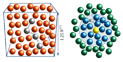
We consider a bead-spring flexible homopolymer with explicit solvent molecules residing in a simple cubic box as shown in the schematic presented in the left panel of Fig. 1. The successive monomers at position of the polymer chain are linearly connected via a bond with energy given by the standard finitely extensible non-linear elastic (FENE) potential
| (2) |
where , the spring constant , equilibrium bond length , and its maximum extension . Both the monomer and solvent molecules are assumed to be spherical beads with diameter and mass . All nonbonded interactions, i.e., solvent-solvent (s-s), solvent-monomer (s-m), and monomer-monomer (m-m) interactions are given by
| (3) |
where is the standard Lennard-Jones (LJ) potential given as
| (4) |
We set and the interaction strength . To facilitate the collapse transition of the polymer we choose the cutoff radius in Eq. (3) in the following way
| (5) |
This implies a purely repulsive potential for s-s and m-m interactions, and a short-range attractive potential for the m-m interaction, mimicking a bad solvent condition for a polymer. On the other hand, a choice of purely repulsive potential by setting for all the above three types of interactions mimics good solvent conditions.
We carry out MD simulations at a constant temperature using the LA thermostat. There, the position and velocity of the -th bead is updated using Newton’s equations
| (6) |
where is the conservative force (originating from the bonded and nonbonded interactions) acting on the particle. The equations of motion are solved using the velocity-Verlet integration scheme. Up to this point the method represents the usual microcanonical MD Frenkel and Smit (2002). To control the temperature using the LA thermostat Lowe (1999); Koopman and Lowe (2006), one considers a pair of particles within a distance as shown in the schematic presented in the right panel of Fig. 1. A heat-bath collision of this pair of particles with a probability is then performed by assigning a new relative velocity to the pair, drawn from the Maxwellian distribution. Here, is the time step and is the collision frequency. The update of relative velocities is only done on the component parallel to the line joining the centers of the pair of particles, thus conserving the angular momentum. Additionally, the new velocities are distributed to the chosen pair in such a way that the linear momentum is also conserved. This makes the thermostat Galilean invariant and hence preserves hydrodynamic effects Lowe (1999); Koopman and Lowe (2006).
The LA approach is an alternative approach to DPD, however, with the liberty to use large in the velocity-Verlet integration scheme Marsh and Yeomans (1997); Nikunen et al. (2003). The other advantage is that by varying and one can tune the bath collision frequency, i.e., effectively controlling the frictional drag or, in other words, the solvent viscosity. We fix and vary over a wide range with the goal to cover solvents of diverse viscosity. This choice of reproduces the known equilibrium properties of a polymer Majumder et al. (2019b).
Following the usual protocol, first, we generate a random walk of length on a simple-cubic lattice and then put this walk or chain in a box of length . Subsequently, we insert solvent particles at random positions keeping the density fixed to and ensure that the solvent particles do not overlap with the monomers of the polymer chain. Then we run our simulations at the desired temperature in good solvent condition [with in Eq. (3)] for MD steps using to get an equilibrated polymer with extended conformation. In our simulations, the unit of temperature is (where we chose ) and the unit of time is the standard LJ time unit . Since we are interested in the collapse kinetics of the polymer, once the system is equilibrated, we change the solvent condition to poor by fixing according to Eq. (5), and let the system evolve as we simultaneously measure various physical quantities that will be presented subsequently. All other parameters remain the same as already stated.
It is easy to perceive that by varying in our simulations one can tune the frictional drag or effectively the solvent viscosity. Hence, subsequently in the rest of the paper we use to represent the solvent viscosity. We systematically vary at different with the goal to encompass a wide range of solvent viscosity. For faster computation we use LAMMPS Plimpton (1995) which we have already modified to implement the LA thermostat Majumder et al. (2019b). We choose polymers of chain length for which the number of solvent particles is roughly the in the range . Except for the snapshots all results presented are averaged over at least different independent initial and thermal realizations generated using different seeds of the random number generator.
III Results
We present the main results by subdividing them into four subsections. In the first subsection, we discuss the overall phenomenology of the collapse, and corresponding analyses required to extract various relaxation times. In the next one we present the scaling of various relaxation times with respect to chain length. In the following two subsections we present, respectively, the temperature and viscosity dependence of various relaxation times.
III.1 Collapse phenomenology and relaxation times
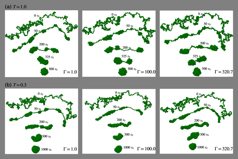
The phenomenology of the collapse following a solvent quench can be understood from the time evolution snapshots, illustrated in Fig. 2 for a polymer of length at two judicially chosen values of the temperature 111Traditionally, the choice of is a more natural choice. Hence in all the figures and tables the data for are always presented first. Also, the otherwise unusual choice of is due to the fact that with our choice of integration time step , for the collision probability of the particles is maximum, i.e., .. For each we show the time evolution for three different values of the solvent viscosity , as indicated. In each case we present typical snapshots at different times starting from an extended coil at to a time where a steady globule is observed. In each case the collapse initiates with the formation of local clusters of monomers along the chain, as shown by the snapshots at . Subsequently these local clusters merge with each other to form bigger clusters and this continues until a single cluster is left. This apparently agrees with the phenomenological picture proposed by HG Halperin and Goldbart (2000). However, a careful inspection of the snapshots across all the presented values of and reveals that only for the higher case, irrespective of , the local clusters of monomers represent true spherical clusters as expected in HG’s pearl-necklace picture. During the course of the collapse at one stage inevitably the polymer attains a dumbbell conformation when only two clusters are present, as represented in Fig. 2(a) by the snapshot at for . Eventually, these two clusters also coalesce with each other and the globule attains an approximate spherical shape.
For the low- case, on the other hand, we observe that the local clusters formed at the initial stages of the collapse do not represent a spherical pearl but rather a sausage-like shape as increases. Thus, the chain resembles a sausage necklace rather than a pearl necklace. Subsequently, the connected sausages coalesce with each other to form longer sausages, and eventually when the last two sausages coalesce the polymer assumes a single cylindrical sausage-like conformation as suggested by de Gennes de Gennes (1985). Following this, the polymer eventually deforms in a slow rearrangement process from the sausage-like conformation to a spherical globule shape. Overall, the inspection of the time evolution snapshots implies that the phenomenology of collapse is dependent on temperature as well as on the solvent viscosity . At high , irrespective of solvent viscosity the phenomenology is purely described by the pearl-necklace picture of HG. On the other hand, at low it is dependent on the solvent viscosity and one observes sausage-like clusters as an intermediate before the polymer attains a spherical shape.
For the first quantitative understanding of the time evolution of the polymer during the collapse we calculate the Euclidean distance between two monomers and as
| (7) |
The variation of is then noted as a function of the contour distance
| (8) |
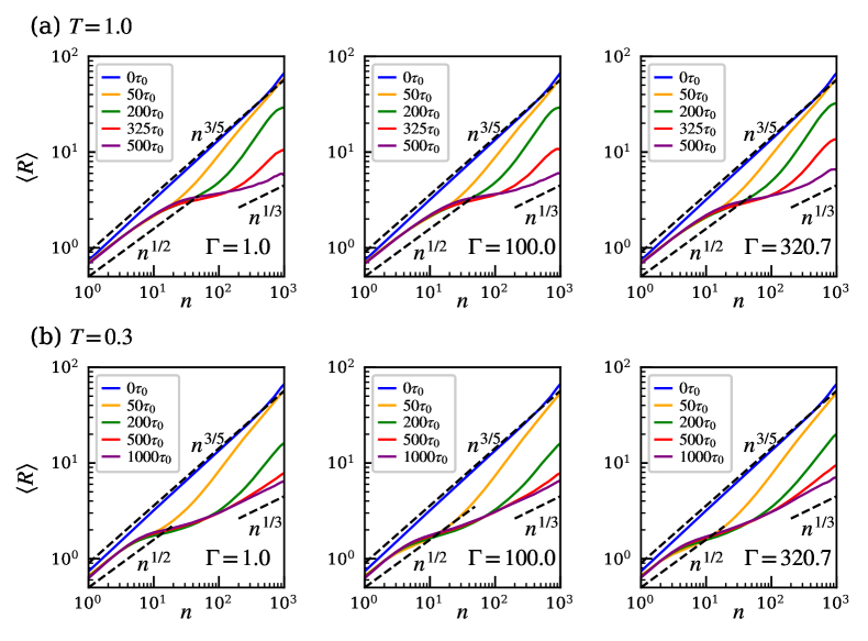
Such plots of at times corresponding to the snapshots in Fig. 2 are presented in Fig. 3. There denotes averaging over different simulation runs and all possible pairs of monomers. It is expected that obeys a power-law scaling of the form de Gennes (1980); Rubenstein and Colby (2003)
| (9) |
The data for , i.e., the starting configuration in all cases of Fig. 3 are consistent with Eq. (9) with an exponent , expected for an extended polymer chain in good solvent de Gennes (1980). Once the solvent condition is changed to poor, the data at large gradually start deviating from the behavior represented by the upper dashed line. At the latest time for large in all cases the data seem to be quite consistent with Eq. (9) with , expected for a globular conformation de Gennes (1980). At large , for small the data seem to be consistent with , i.e., a Gaussian behavior. This can be understood by considering the pearls or globules to be made up of several small segments of the polymer itself. Each of these segments feels the highly dense surrounding consisting of all the other segments, effectively mimicking a polymer-melt like environment where a Gaussian behavior is expected de Gennes (1980). The agreement of the data with the expected scaling at early and late times confirm the formation of globule-like conformation through collapse of an extended coil-like conformation, irrespective of the temperature and solvent viscosity . However, no signature of the different collapse pathways as identified from the time evolution snapshots in Fig. 2 is resolved.
Following the traditional approach to monitor the kinetics we also calculate the squared radius of gyration
| (10) |
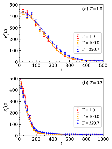
The corresponding time dependence of is presented in Fig. 4 for the systems presented in Figs. 2 and 3. At both , the data for different apparently do not imply any general trend. Also, the decay of with time does not provide clear signature of the intermediate stages of the collapse. Nevertheless, we extract a relaxation time proportional to the overall collapse time by fitting the curves with the following stretched exponential function
| (11) |
where corresponds to of the collapsed conformation, and and are associated nontrivial fitting parameters. The results of the fitting exercises on the data presented in Fig. 4 are tabulated in Table 1. The obtained relaxation times for both have no clear systematic trend as a function of . The value of indicates a faster collapse at , contradicting with the actual fact revealed from the time evolution snapshots in Fig. 2 which gives a clear indication that the overall collapse time, i.e., the time it takes to form a spherical globule from an extended coil, increases as decreases. Also note the difference in the values of , which correspond to the respective equilibrium value of at the two . At one notices a drop in the value of as solvent viscosity changes from to , suggesting a faster collapse in viscous solvent. This is also not in agreement with the picture reflected by the time evolution snapshots at in Fig. 2. Furthermore, the values of quoted in Table 1 are also significantly higher than the previously reported values obtained from Monte Carlo simulations of a homopolymer collapse without explicit solvent Majumder et al. (2017); Christiansen et al. (2017). Overall, it can be inferred that the traditional approach of extracting the relaxation times using the decay of is not unambiguous in the present case. Importantly, it cannot be used to draw any information on the time scales that separate different stages of the collapse, especially the transition from the pearl-necklace-like to the sausage-like picture at low .
The variety of conformations observed for a polymer during its collapse as presented in Fig. 2 motivates us now to investigate various shape properties of the polymer. For equilibrium conformations of polymer, shape properties have proven to be useful tools in identifying various structural transitions Alim and Frey (2007); Ostermeir et al. (2010); Blavatska and Janke (2010); Arkın and Janke (2013). With this motivation we first calculate the full gyration tensor having the components
| (12) |
where is the -th component of the center-of-mass vector
| (13) |
We move onto calculating various shape properties derived from . The spread in eigenvalues of gives an idea about how uniformly the monomers of the polymer are distributed spatially, and thus measures the asymmetry of the chain. Various combination of the eigenvalues provide different useful measures of the asymmetry present in the polymer conformation. To proceed further, we first calculate the mean eigenvalue
| (14) |
This allows us to calculate the extent of asphericity of a conformation Theodorou and Suter (1985); Aronovitz and Nelson (1986); Cannon et al. (1991); Blavatska and Janke (2010); Arkın and Janke (2013)
| (15) |
where with being the unity matrix. can be used to distinguish shapes of different polymer conformations. For example for a completely spherical conformation and for perfectly rod-like conformation. For any polymer conformation it obeys the bounds . We also calculate the prolateness of a polymer conformation as Aronovitz and Nelson (1986); Blavatska and Janke (2010); Arkın and Janke (2013)
| (16) |
For an absolute prolate conformation, i.e., for a rod , implying that . For an absolute oblate conformation, i.e., for a disk , , implying . Thus, the bounds are . We also calculate another quantity defined as the nature of asphericity Cannon et al. (1991); Alim and Frey (2007); Ostermeir et al. (2010)
| (17) |
For a disk, , whereas for a rigid rod . Thus the nature of asphericity has the bounds . Note that the so far described parameters , , and are all rotationally invariant and universal quantities Aronovitz and Nelson (1986); Cannon et al. (1991).
Apart from the above parameters one can also consider certain parameters which are not invariant. For that one needs to sort the eigenvalues in descending order which allows us to define as a simple parameter the asphericity Theodorou and Suter (1985)
| (18) |
Similarly, as another simple parameter we calculate the acylindricity Theodorou and Suter (1985)
| (19) |
For a perfectly spherical object, all eigenvalues are equal and hence , while a large positive value of indicates strong asphericity. For shapes of tetrahedral or even higher symmetry , and for a perfect cylinder . Note that and can be obtained only from the eigenvalues of .
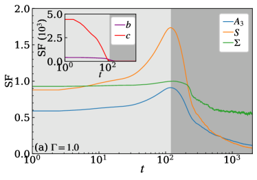
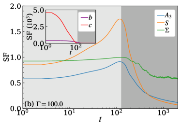
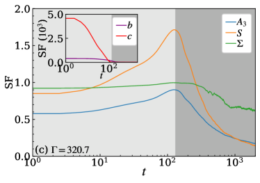
Utility of various shape factors in disentangling different stages of the collapse of a polymer in solvents of varying viscosity at is illustrated in Fig. 5. In the main frame we show plots for the invariant shape parameters , , and , while the simple but not invariant ones are shown in the insets. Both and appear to nicely capture the two distinct stages of the overall collapse process. They start off at the respective initial values for an extended coil. At very early time , the behaviors are almost flat marking the formation of stable clusters. In the range both and show steady rise highlighting the pearl-necklace stage. Eventually, they approach a maximum when all clusters have merged to form a single cluster, which at low resembles a sausage-like conformation. In the next stage the sausage starts relaxing via rearrangement of the monomers and then both and start decaying from their maximum values to approach zero, the value for a perfectly spherical globule. Even though also shows a similar behavior as a function of time, it is difficult to pin-point the end of the pearl-necklace stage from it due to the absence of any prominent maxima in the data. Also at very late time for all , the data for almost saturate indicating no change in the conformation. However, by inspecting the conformation around that time it is clear that the conformation is still relaxing. This feature is clearly visible in the data of both and . Thus, and will not only allow us to extract a time scale for the end of the pearl-necklace stage but can also potentially be used for estimating a relaxation time for the sausage stage. This will be done subsequently. The simpler quantities and also approach zero starting from a high value, reflecting the transition from the pearl-necklace to sausage stage. However, like both and do not show any significant features in the sausage stage that would allow one to extract a relaxation time for the sausage stage. Thus based on the above discussion it seems that both and are the two potential parameters that can be used to extract the relaxation times related to the different stages of the collapse. However, from now on we will be using only with the rational that in principle uniquely identifies a spherical object, whereas approaching its lower bound ideally indicates a disk-like object.
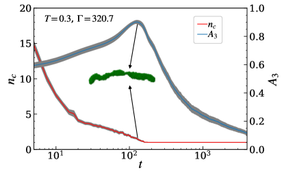
To further substantiate our choice of , we show in Fig. 6 its compatibility with the time dependence of the number of clusters of monomers formed in the pear-necklace stage of the collapse. For determining , we first calculate the number of monomers present within a cut-off distance of the -th monomer as
| (20) |
where is the Heaviside step function. For, , we consider that there is a cluster around the -th monomer and all the monomers are part of that cluster. Here, we choose . This way the number of clusters may be overcounted, which we remove via a Venn diagram approach to find the actual number of discrete clusters . For the details on identifying and counting the number of clusters see Ref. Majumder et al. (2020). The data for are nicely synchronized with the data presented in Fig. 6 for a polymer of at collapsing in a solvent of viscosity . The point where the data attain its maximum nicely coincides with the point when for the first time. Thus, it is evident that can be relied on to extract the relaxation time marking the crossover from pearl-necklace to sausage-like phenomenology of the collapse. Thus we use the time where the data attain the peak value as a measure of the pearl-necklace relaxation time . Following the pearl-necklace stage, the data remain constant at unity, but the data start decaying from its peak value and continue to do so characterizing the sausage relaxation.
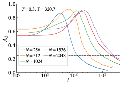
In Fig. 7 we show variation of the time dependence of the data during the collapse with length of the polymer in a solvent with viscosity at . One can clearly notice a monotonic dependence of the peak position with , a signature of increasing with as expected. Similarly, one can also notice a slower decay of the data following the peak. This observation allows us to obtain an overall collapse time given as
| (21) |
We have checked that any value of in the range provides proportionate results for . Subsequently, all the values presented are for the choice , as represented by the dashed line in Fig. 7. Now from the obtained and we determine the sausage relaxation time
| (22) |
III.2 Scaling of relaxation times with chain length
With the methods for extracting various relaxation times in place, we first move on to investigate their scaling with respect to the length of the polymer. For that we use simulations at two fixed temperatures and three fixed solvent viscosities for five different chain lengths.
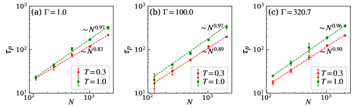
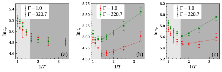
The obtained relaxation times are presented in the log-log plots of Fig. 8 as a function of , at a low and a high for different . The data for the relaxation time characterizing the pearl-necklace stage, shown in the first row (a)-(c) show a power-law scaling of the form
| (23) |
where is the corresponding dynamic exponent. The dashed lines in Figs. 8(a)-(c) represent the best fit lines obtained after fitting the form in Eq. (23) to the data. The detail results of the fitting are presented in Table 2. It seems that is almost independent of at . For , the dynamics seems to be faster with smaller value of , however, showing a slight increase as a function of . The faster dynamics at low is an effect of the fact that the solvent becomes poorer with decreasing , as previously also observed for the overall collapse time in cases where only the pearl-necklace stage is present in the collapse Majumder et al. (2017).
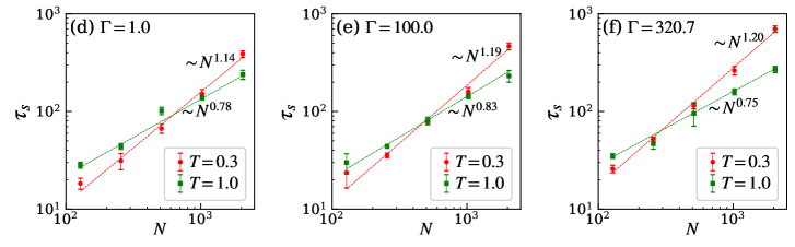
The corresponding scaling plots of the sausage relaxation time are presented in Figs. 8(d)-(f). There also the data seem to be following a power-law scaling which allows to perform a fitting using the ansatz
| (24) |
The resulting parameters are compiled in Table 3. For both the data are weakly dependent on the solvent viscosity with and for and , respectively, indicating that the dynamics is faster at high unlike the pearl-necklace relaxation. This is due to fact that the relaxation in the sausage stage occurs via hydrodynamic dissipation of the surface energy, which gets accelerated with increasing de Gennes (1985).
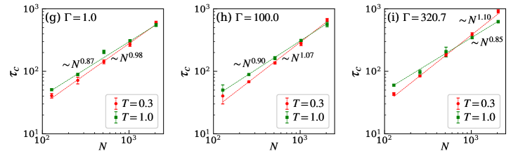
Finally we show the scaling of the overall collapse time in Figs. 8(g)-(i). Again the data show a nice power-law scaling which we quantify using the usual ansatz of the form
| (25) |
Results of the fitting exercise using (25) are quoted in Table 4. The data at indicate that the corresponding dynamic exponent is nonmonotonic with the variation of , whereas at suggests a very weak dependence. As a function of the trend in the data is similar to what is observed for suggesting that the sausage relaxation is the rate-limiting stage of the overall collapse process. Overall the data suggest that the scaling of also is dependent on . The inclusion of solvent viscosity introduces a temperature-dependent frictional drag by the solvent molecules while the polymer tries to move, thus making the scaling of the relaxation times with the chain length a function of temperature.
III.3 Temperature dependence of the relaxation times
In this subsection we present results for the dependence of the relaxation times on temperature. For that we perform simulations at eight different using a polymer of fixed length for two fixed solvent viscosities.
Considering the analogy between the collapse of a homopolymer and hydrophobic collapse or protein folding in general, it is to be noted that the folding rates of most proteins show Arrhenius behavior Scalley and Baker (1997). Similarly, to classify structural glasses into fragile and non-fragile categories, one often checks whether the relaxation time follows an Arrhenius behavior. In terms of the Arrhenius behavior is given as
| (26) |
where is the amplitude and is the activation energy. On taking logarithm, Eq. (26) transforms to
| (27) |
Thus, a linear behavior of the plot of as a function of confirms an Arrhenius behavior.
In Fig. 9 we present a test of the Arrhenius behavior of the relaxation times corresponding to the two stages of the collapse and the overall collapse time. Over the considered range the data for in Fig. 9(a) show no signature of the Arrhenius behavior. At low it indicates no dependence on the temperature. On the other hand, in the high- range (marked by the lighter shade) it rather increases almost linearly with suggesting an anti-Arrhenius behavior, also observed in folding dynamics of certain proteins Munoz et al. (1997); Karplus (2000); Ferrara et al. (2000). Since the range in is not sufficiently long we abstain ourselves from fitting a straight line. Considering the fact that as increases the poor solvent approaches a good one, it is expected that the formation of small clusters or pearls of monomers slows down.
In the high- range similar behavior is observed for the sausage relaxation time presented in Fig. 9(b), however, the range of (marked by the lighter shade) seems to have shrinked. In the low- range the data for both clearly indicate a linear behavior with positive slope suggesting an Arrhenius behavior. This indulges us to fit Eq. (27) to the data, results of which are tabulated in Table 5. The dashed lines passing over the data points are the respective best fit straight lines obtained from this fitting exercise confirming the Arrhenius behavior. From the results obtained via fitting it appears that the amplitude is independent of , whereas the activation energy for the sausage relaxation is larger for larger .
The data for the overall collapse time presented in Fig. 9(c) as a function of show almost the same behavior as the sausage relaxation time . This again confirms that for the overall collapse the sausage relaxation is the rate-limiting stage. However, the high- range for the anti-Arrhenius behavior coincides with the data for . Results from the fitting exercise with the Arrhenius behavior in Eq. (27) are also presented in Table 5. The corresponding best fit lines are represented by the dashed lines passing over the data points. The fit values obtained once again infer that the amplitude is independent of the solvent viscosity . The corresponding activation energy is apparently larger for larger . According to the error bars, the range of the ratio of obtained for and varies from to for the values extracted from . For the values extracted from , the corresponding ratio spans a much wider range from to . Due to the wider range for it would not be advisable to extract the activation energy from it. On the other hand, the values extracted from with a narrow range provides a more reliable measure of the activation energy of the overall collapse process. This can also be appreciated from the fact that the sausage relaxation is the bottle neck of the overall collapse process.
III.4 Solvent-viscosity dependence of the relaxation times
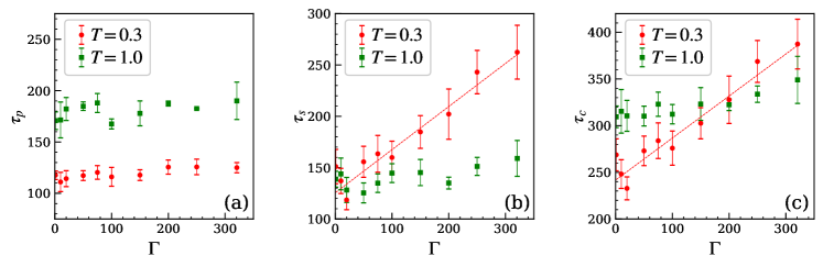
Finally we present results for the dependence of the relaxation times on the solvent viscosity . For that we perform simulations at ten different for a polymer of fixed length at two fixed temperatures.
The obtained dependence of the relaxation times as a function of are shown in Fig. 10. The pearl necklace relaxation time presented in Fig. 10(a) shows no dependency on the solvent viscosity for both temperatures. This can be intuitively derived from the fact that in the pearl-necklace stage local ordering of the monomers is the driving force which presumably depends negligibly on the solvent viscosity. On the other hand, the sausage relaxation occurs via the minimization of the surface energy which gets opposed by the motion of the solvent molecules, unless there are sufficient thermal fluctuations to cross that barrier. This is reflected by the dependence of the sausage relaxation time on the solvent viscosity , presented in Fig. 10(b). The apparent linear behavior of the data for calls for a fit using the following ansatz
| (28) |
where represent the relaxation time due to the internal friction of the polymer and is the amplitude for the dependence on the solvent viscosity . The ansatz in Eq. (28) is commonly used for viscosity dependence of folding rates of proteins Qiu and Hagen (2004); Schulz et al. (2012); Zheng et al. (2015). There, the linear behavior is originally motivated by drawing analogy between protein folding and chemical reactions in solution, and thereby using the Kramer’s theory of linear dependency of folding relaxation times and the solvent viscosity Kramers (1940). The dashed line in Fig. 10(b) is the best fit resulting from fitting Eq. (28) with the data for . The corresponding values are and . One of course could argue about a fit using a pure power-law of the form . For protein folding it has been argued Qiu and Hagen (2004); Schulz et al. (2012) that such a power-law dependence requires the relaxation rate to diverge at vanishing solvent viscosity, whereas an ansatz of the form (28) implies that another damping mechanism intercedes to control the folding rate as friction due to solvent vanishes. With hindsight and topped up by the apparent linear behavior of with at , we abstain ourselves from using a power-law fit to the data. At the data for shows negligible dependence on since the thermal fluctuations are sufficiently strong to overcome the barrier due to friction of solvent molecules.
In Fig. 10(c) we show the dependence of the overall collapse time on the solvent viscosity . Since the sausage relaxation is the rate-limiting stage of the overall collapse process, the behavior of is similar to what is observed for . This compels us to analyze the data at using the linear ansatz analogous to (28)
| (29) |
A fit with the above form to the data yields and . Note that the obtained suggesting that the amplitude for dependence on solvent viscosity is rather robust. The data for show negligible dependence on as observed for .
IV Conclusion
We have presented results exploring the nonequilibrium pathways of the collapse transition of a flexible homopolymer when it is quenched from its extended coil state in a good solvent to a poor solvent where the equilibrium conformation is a compact globule. We have performed simulations considering explicit solvent molecules in a framework using the Lowe-Andersen thermostat which allowed us to tune the solvent viscosity . Results from our simulations over a wide range of and at different temperatures revealed new insights about the collapse pathway. For moderate to high the collapse occurs through pearl-necklace intermediates in accordance with the Halperin-Goldbart picture, independent of the solvent viscosity as observed in previous simulations without considering solvent viscosity. Interestingly, at low our results confirm the de Gennes prediction that following the pearl-necklace stage the polymer attains a distinct sausage-like conformation which subsequently, via minimization of the surface energy, approaches a compact spherical globule. Presence of the sausage-like intermediates gets prolonged with increase of the solvent viscosity . This brings us to the conjecture that the collapse pathway of a polymer is a function of the temperature and solvent viscosity, depending on which one observes initially the pearl-necklace intermediate followed by the sausage intermediates.
Since the usual protocol of understanding the collapse dynamics was not adequate, we have used different shape factors derived from the gyration tensor to disentangle the pearl-necklace and the sausage relaxation stages. This also allowed us to extract the respective relaxation times of the two stages of the collapse as well as the overall collapse time. Both the pearl-necklace relaxation time and the sausage relaxation time show power-law scaling as a function of the polymer length . A smaller value of the power-law exponent for at low suggests a faster dynamics of the pearl-necklace stage as a courtesy of the fact that the solvent becomes poorer with decrease in . Conversely, the power-law exponent indicates that the dynamics of the sausage relaxation is faster at higher . This is in accordance with de Gennes phenomenological picture suggesting that the minimization of the surface energy of the sausage-like intermediates occurring via hydrodynamic dissipation of energy is faster at high . The overall collapse time shows similar scaling behavior as implying that the sausage relaxation is the rate-limiting stage in the overall collapse process of the polymer.
We have shown that for a fixed , all the relaxation times show an anti-Arrhenius behavior in the high- range. In the low- regime, whereas is almost insensitive to , both and follow Arrhenius behavior from where one can extract the corresponding activation energy of the sausage relaxation and the overall collapse. For a fixed and , results for varying solvent viscosity showed that the pearl-necklace relaxation dynamics is independent of . At low , dependence of on have shown a linear behavior, similar to what is found for folding rates of proteins. The agreement of the data to a straight line with an off-set is further indicative of the existence of internal friction of the polymer. This implies that internal friction of proteins could plausibly originating from its polymeric backbone rather than depending on the specifics of its sequence. A study of semiflexible heteropolymers using the framework of the present work would be able to shed more light on this, which we take up as a our next endeavor 222H. Christiansen, S. Majumder, and W. Janke, work in progress.
In future, it would be interesting to study the dependence of the cluster coarsening on the solvent viscosity. Intriguing would also be to investigate the role of solvent viscosity in the aging and related scaling during the collapse. Polymers are found to be residing in a different, confined geometrical setup in the real world. Hence, it would be worth exploring both the equilibrium and nonequilibrium dynamics of a polymer in restricted geometries using our current simulation setup. Going by the recent trend of investigating biomolecules as active entities, it would certainly be promising to study active polymers in this explicit solvent setup where the solvent viscosity can be tuned.
Acknowledgements.
S.M. was funded by the Science and Engineering Research Board (SERB), Govt. of India through a Ramanujan Fellowship (File no. RJF/2021/000044). W.J. thanks funding by the Deutsche Forschungsgemeinschaft (DFG, German Research Foundation) – 469 830 597 under project ID JA 483/35-1.References
- Onuchic et al. (1997) J.N. Onuchic, Z. Luthey-Schulten, and P.G. Wolynes, “Theory of protein folding: The energy landscape perspective,” Ann. Rev. Phys. Chem. 48, 545–600 (1997).
- Shakhnovich (2006) E. Shakhnovich, “Protein folding thermodynamics and dynamics: where physics, chemistry, and biology meet,” Chem. Rev. 106, 1559–1588 (2006).
- Dill et al. (2008) K.A. Dill, S.B. Ozkan, M.S. Shell, and T.R. Weikl, “The protein folding problem,” Annu. Rev. Biophys. 37, 289–316 (2008).
- Dill and MacCallum (2012) K.A. Dill and J.L. MacCallum, “The protein-folding problem, 50 years on,” Science 338, 1042–1046 (2012).
- Jumper et al. (2021) J. Jumper, R. Evans, A. Pritzel, T. Green, M. Figurnov, O. Ronneberger, K. Tunyasuvunakool, R. Bates, A. Žídek, A. Potapenko, et al., “Highly accurate protein structure prediction with AlphaFold,” Nature 596, 583–589 (2021).
- Bhatia and Udgaonkar (2022) S. Bhatia and J.B. Udgaonkar, “Heterogeneity in protein folding and unfolding reactions,” Chem. Rev. 122, 8911–8935 (2022).
- Camacho and Thirumalai (1993) C.J. Camacho and D. Thirumalai, “Kinetics and thermodynamics of folding in model proteins,” Proc. Natl. Acad. Sci. U.S.A. 90, 6369 (1993).
- Pollack et al. (2001) L. Pollack, M.W. Tate, A.C. Finnefrock, C. Kalidas, S. Trotter, N.C. Darnton, L. Lurio, R.H. Austin, C.A. Batt, S.M. Gruner, and S.G.J. Mochrie, “Time Resolved Collapse of a Folding Protein Observed with Small Angle X-Ray Scattering,” Phys. Rev. Lett. 86, 4962 (2001).
- Sadqi et al. (2003) M. Sadqi, L.J. Lapidus, and V. Muñoz, “How fast is protein hydrophobic collapse?” Proc. Natl. Acad. Sci. U.S.A. 100, 12117 (2003).
- Haran (2012) G. Haran, “How, when and why proteins collapse: The relation to folding,” Curr. Opin. Struct. Bio.. 22, 14–20 (2012).
- Reddy and Thirumalai (2017) G. Reddy and D. Thirumalai, “Collapse precedes folding in denaturant-dependent assembly of ubiquitin,” J. Phys. Chem. B 121, 995 (2017).
- Nishio et al. (1979) I. Nishio, S.-T. Sun, G. Swislow, and T. Tanaka, “First observation of the coil–globule transition in a single polymer chain,” Nature 281, 208 (1979).
- de Gennes (1985) P.-G. de Gennes, “Kinetics of collapse for a flexible coil,” J. Phys. Lett. 46, 639 (1985).
- Yu et al. (1992) J. Yu, Z. Wang, and B. Chu, “Kinetic study of coil-to-globule transition,” Macromolecules 25, 1618–1620 (1992).
- Grosberg and Kuznetsov (1993) A.Y. Grosberg and D.V. Kuznetsov, “Single-chain collapse or precipitation? Kinetic diagram of the states of a polymer solution,” Macromolecules 26, 4249–4251 (1993).
- Byrne et al. (1995) A. Byrne, P. Kiernan, D. Green, and K.A. Dawson, “Kinetics of homopolymer collapse,” J. Chem. Phys. 102, 573 (1995).
- Timoshenko et al. (1995) E.G. Timoshenko, Y.A. Kuznetsov, and K.A. Dawson, “Kinetics at the collapse transition: Gaussian self-consistent approach,” J. Chem. Phys. 102, 1816–1823 (1995).
- Kuznetsov et al. (1995) Y.A. Kuznetsov, E.G. Timoshenko, and K.A. Dawson, “Kinetics at the collapse transition of homopolymers and random copolymers,” J. Chem. Phys. 103, 4807–4818 (1995).
- Kuznetsov et al. (1996a) Y.A. Kuznetsov, E.G. Timoshenko, and K.A. Dawson, “Kinetic laws at the collapse transition of a homopolymer,” J. Chem. Phys. 104, 3338–3347 (1996a).
- Kuznetsov et al. (1996b) Y.A. Kuznetsov, E.G. Timoshenko, and K.A. Dawson, “Equilibrium and kinetic phenomena in a stiff homopolymer and possible applications to DNA,” J. Chem. Phys. 105, 7116–7134 (1996b).
- Klushin (1998) L.I. Klushin, “Kinetics of a homopolymer collapse: Beyond the Rouse–Zimm scaling,” J. Chem. Phys. 108, 7917–7920 (1998).
- Halperin and Goldbart (2000) A. Halperin and P.M. Goldbart, “Early stages of homopolymer collapse,” Phys. Rev. E 61, 565 (2000).
- Hagen and Eaton (2000) S.J. Hagen and W.A. Eaton, “Two-state expansion and collapse of a polypeptide,” J. Mol. Biol. 301, 1019–1027 (2000).
- Abrams et al. (2002) C.F. Abrams, N.-K. Lee, and S.P. Obukhov, “Collapse dynamics of a polymer chain: Theory and simulation,” Europhys. Lett. 59, 391 (2002).
- Montesi et al. (2004) A. Montesi, M. Pasquali, and F.C. MacKintosh, “Collapse of a semiflexible polymer in poor solvent,” Phys. Rev. E 69, 021916 (2004).
- Kikuchi et al. (2005) N. Kikuchi, J.F. Ryder, C.M. Pooley, and J.M. Yeomans, “Kinetics of the polymer collapse transition: The role of hydrodynamics,” Phys. Rev. E 71, 061804 (2005).
- Xu et al. (2006) J. Xu, Z. Zhu, S. Luo, C. Wu, and S. Liu, “First Observation of Two-stage Collapsing Kinetics of a Single Synthetic Polymer Chain,” Phys. Rev. Lett. 96, 027802 (2006).
- Ye et al. (2007) X. Ye, Y. Lu, L. Shen, Y. Ding, S. Liu, G. Zhang, and C. Wu, “How many stages in the coil-to-globule transition of linear homopolymer chains in a dilute solution?” Macromolecules 40, 4750–4752 (2007).
- Pham et al. (2008) T.T. Pham, M. Bajaj, and J.R. Prakash, “Brownian dynamics simulation of polymer collapse in a poor solvent: Influence of implicit hydrodynamic interactions,” Soft Matter 4, 1196–1207 (2008).
- Guo et al. (2011) J. Guo, H. Liang, and Z.-G. Wang, “Coil-to-globule transition by dissipative particle dynamics simulation,” J. Chem. Phys. 134, 244904 (2011).
- Udgaonkar (2013) J.B. Udgaonkar, “Polypeptide chain collapse and protein folding,” Arch. Biochem. Biophys. 531, 24–33 (2013).
- Majumder and Janke (2015) S. Majumder and W. Janke, “Cluster coarsening during polymer collapse: Finite-size scaling analysis,” Europhys. Lett. 110, 58001 (2015).
- Majumder and Janke (2016a) S. Majumder and W. Janke, “Evidence of aging and dynamic scaling in the collapse of a polymer,” Phys. Rev. E 93, 032506 (2016a).
- Majumder et al. (2017) S. Majumder, J. Zierenberg, and W. Janke, “Kinetics of polymer collapse: Effect of temperature on cluster growth and aging,” Soft Matter 13, 1276 (2017).
- Christiansen et al. (2017) H. Christiansen, S. Majumder, and W. Janke, “Coarsening and aging of lattice polymers: Influence of bond fluctuations,” J. Chem. Phys. 147, 094902 (2017).
- Majumder et al. (2019a) S. Majumder, U.H.E. Hansmann, and W. Janke, “Pearl-necklace-like local ordering drives polypeptide collapse,” Macromolecules 52, 5491–5498 (2019a).
- Majumder et al. (2020) S. Majumder, H. Christiansen, and W. Janke, “Understanding nonequilibrium scaling laws governing collapse of a polymer,” Euro. Phys. J. B 93, 142 (2020).
- Schneider et al. (2020) J. Schneider, M.K. Meinel, H. Dittmar, and F. Müller-Plathe, “Different stages of polymer-chain collapse following solvent quenching–scaling relations from dissipative particle dynamics simulations,” Macromolecules 53, 8889–8900 (2020).
- Rubenstein and Colby (2003) M. Rubenstein and R.H. Colby, Polymer Physics (Chemistry) (Oxford University Press, Oxford, 2003).
- Majumder and Janke (2016b) S. Majumder and W. Janke, “Aging and related scaling during the collapse of a polymer,” J. Phys.: Conf. Ser. 750, 012020 (2016b).
- Malevanets and Kapral (1999) A. Malevanets and R. Kapral, “Mesoscopic model for solvent dynamics,” J. Chem. Phys. 110, 8605–8613 (1999).
- Hoogerbrugge and Koelman (1992) P.J. Hoogerbrugge and J.M.V.A. Koelman, “Simulating microscopic hydrodynamic phenomena with dissipative particle dynamics,” Europhys. Lett. 19, 155 (1992).
- Espanol and Warren (1995) P. Espanol and P.B. Warren, “Statistical mechanics of dissipative particle dynamics,” Europhys. Lett. 30, 191 (1995).
- Groot and Warren (1997) R.D. Groot and P.B. Warren, “Dissipative particle dynamics: Bridging the gap between atomistic and mesoscopic simulation,” J. Chem. Phys. 107, 4423–4435 (1997).
- Klimov and Thirumalai (1997) D.K. Klimov and D. Thirumalai, “Viscosity Dependence of the Folding Rates of Proteins,” Phys. Rev. Lett. 79, 317 (1997).
- Zagrovic and Pande (2003) B. Zagrovic and V. Pande, “Solvent viscosity dependence of the folding rate of a small protein: Distributed computing study,” J. Comput. Chem. 24, 1432–1436 (2003).
- Rhee and Pande (2008) Y.M. Rhee and V.S. Pande, “Solvent viscosity dependence of the protein folding dynamics,” J. Phys. Chem. B 112, 6221–6227 (2008).
- Hagen (2010) S.J. Hagen, “Solvent viscosity and friction in protein folding dynamics,” Curr. Pro. Pept. Sci. 11, 385–395 (2010).
- De Sancho et al. (2014) D. De Sancho, A. Sirur, and R.B. Best, “Molecular origins of internal friction effects on protein-folding rates,” Nat. Comm. 5, 4307 (2014).
- Zheng et al. (2015) W. Zheng, D. De Sancho, T. Hoppe, and R.B. Best, “Dependence of internal friction on folding mechanism,” J. Am. Chem. Soc. 137, 3283–3290 (2015).
- Lowe (1999) C.P. Lowe, “An alternative approach to dissipative particle dynamics,” Europhys. Lett. 47, 145 (1999).
- Koopman and Lowe (2006) E.A. Koopman and C.P. Lowe, “Advantages of a Lowe-Andersen thermostat in molecular dynamics simulations,” J. Chem. Phys. 124, 204103 (2006).
- Frenkel and Smit (2002) D. Frenkel and B. Smit, Understanding Molecular Simulations: From Algorithms to Applications (Academic Press, San Diego, 2002).
- Marsh and Yeomans (1997) C.A. Marsh and J.M. Yeomans, “Dissipative particle dynamics: The equilibrium for finite time steps,” Europhys. Lett. 37, 511 (1997).
- Nikunen et al. (2003) P. Nikunen, M. Karttunen, and I. Vattulainen, “How would you integrate the equations of motion in dissipative particle dynamics simulations?” Comput. Phys. Commun. 153, 407–423 (2003).
- Majumder et al. (2019b) S. Majumder, H. Christiansen, and W. Janke, “Dissipative dynamics of a single polymer in solution: A Lowe-Andersen approach,” J. Phys.: Conf. Ser. 1163, 012072 (2019b).
- Plimpton (1995) S. Plimpton, “Fast parallel algorithms for short-range molecular dynamics,” J. Comput. Phys. 117, 1–19 (1995).
- Note (1) Traditionally, the choice of is a more natural choice. Hence in all the figures and tables the data for are always presented first. Also, the otherwise unusual choice of is due to the fact that with our choice of integration time step , for the collision probability of the particles is maximum, i.e., .
- de Gennes (1980) P.-G. de Gennes, Scaling Concepts in Polymer Physics (AIP, Melville, New York, 1980).
- Alim and Frey (2007) K. Alim and E. Frey, “Shapes of Semiflexible Polymer Rings,” Phys. Rev. Lett. 99, 198102 (2007).
- Ostermeir et al. (2010) K. Ostermeir, K. Alim, and E. Frey, “Buckling of stiff polymer rings in weak spherical confinement,” Phys. Rev. E 81, 061802 (2010).
- Blavatska and Janke (2010) V. Blavatska and W. Janke, “Shape anisotropy of polymers in disordered environment,” J. Chem. Phys. 133, 184903 (2010).
- Arkın and Janke (2013) H. Arkın and W. Janke, “Gyration tensor based analysis of the shapes of polymer chains in an attractive spherical cage,” J. Chem. Phys. 138, 054904 (2013).
- Theodorou and Suter (1985) D.N. Theodorou and U.W. Suter, “Shape of unperturbed linear polymers: Polypropylene,” Macromolecules 18, 1206–1214 (1985).
- Aronovitz and Nelson (1986) J.A. Aronovitz and D.R. Nelson, “Universal features of polymer shapes,” J. Phys. (Paris) 47, 1445–1456 (1986).
- Cannon et al. (1991) J.W. Cannon, J.A. Aronovitz, and P. Goldbart, “Equilibrium distribution of shapes for linear and star macromolecules,” J. Phys. I 1, 629–645 (1991).
- Scalley and Baker (1997) M.L. Scalley and D. Baker, “Protein folding kinetics exhibit an Arrhenius temperature dependence when corrected for the temperature dependence of protein stability,” Proc. Nat. Acad. Sci. U.S.A. 94, 10636–10640 (1997).
- Munoz et al. (1997) V. Munoz, P.A. Thompson, J. Hofrichter, and W.A. Eaton, “Folding dynamics and mechanism of -hairpin formation,” Nature 390, 196–199 (1997).
- Karplus (2000) M. Karplus, “Aspects of protein reaction dynamics: Deviations from simple behavior,” J. Phys. Chem. B 104, 11–27 (2000).
- Ferrara et al. (2000) P. Ferrara, J. Apostolakis, and A. Caflisch, “Thermodynamics and kinetics of folding of two model peptides investigated by molecular dynamics simulations,” J. Phys. Chem. B 104, 5000–5010 (2000).
- Qiu and Hagen (2004) L. Qiu and S.J. Hagen, “Internal friction in the ultrafast folding of the tryptophan cage,” Chem. Phys. 307, 243–249 (2004).
- Schulz et al. (2012) J.C.F. Schulz, L. Schmidt, R.B. Best, J. Dzubiella, and R.R. Netz, “Peptide chain dynamics in light and heavy water: Zooming in on internal friction,” J. Am. Chem. Soc. 134, 6273–6279 (2012).
- Kramers (1940) H.A. Kramers, “Brownian motion in a field of force and the diffusion model of chemical reactions,” Physica 7, 284–304 (1940).
- Note (2) H. Christiansen, S. Majumder, and W. Janke, work in progress.