A general error analysis for randomized low-rank approximation with application to data assimilation††thanks: This work was funded by ISAE-SUPAERO, France.
Abstract
Randomized algorithms have proven to perform well on a large class of numerical linear algebra problems. Their theoretical analysis is critical to provide guarantees on their behaviour, and in this sense, the stochastic analysis of the randomized low-rank approximation error plays a central role. Indeed, several randomized methods for the approximation of dominant eigen- or singular modes can be rewritten as low-rank approximation methods. However, despite the large variety of algorithms, the existing theoretical frameworks for their analysis rely on a specific structure for the covariance matrix that is not adapted to all the algorithms. We propose a general framework for the stochastic analysis of the low-rank approximation error in Frobenius norm for centered and non-standard Gaussian matrices. Under minimal assumptions on the covariance matrix, we derive accurate bounds both in expectation and probability. Our bounds have clear interpretations that enable us to derive properties and motivate practical choices for the covariance matrix resulting in efficient low-rank approximation algorithms. The most commonly used bounds in the literature have been demonstrated as a specific instance of the bounds proposed here, with the additional contribution of being tighter. Numerical experiments related to data assimilation further illustrate that exploiting the problem structure to select the covariance matrix improves the performance as suggested by our bounds.
Keywords: Low-rank approximation methods, randomized algorithms, Singular Value Decomposition, non-standard Gaussian error analysis, data assimilation.
MSCcodes: 65F55, 65F99, 65K99, 68W20.
1 Introduction
Let be an arbitrary real matrix and consider the following minimization problem,
| (1.1) |
where denotes the Frobenius norm. This problem, referred to as the low-rank approximation problem, is a key ingredient in numerous applications in data analysis and scientific computing including principal component analysis [23], data compression [19] and approximation algorithms for partial differential and integral equations [13], to name a few. Its solution [7] is obtained from the order truncated singular value decomposition (SVD) of .
Let and be the real orthogonal matrices containing the left and right singular vectors of respectively, and the matrix containing the singular values of with the convention . For a given integer , we consider the following partitioning of the SVD of ,
| (1.2) |
where , , , , and . Defining and , one can rewrite where the matrix is precisely the solution of (1.1). The corresponding optimal value reads .
The matrix can be computed with any SVD algorithm enabling a truncation mechanism [8, Section 9.6]. However, for large-scale problems, the classical approaches become prohibitively expensive or are even inapplicable if is not stored explicitly. In these situations, one is rather interested in computing , a reasonably accurate approximation of , which is typically expected to be optimal up to a small factor , that is, satisfies,
Over the past decade, randomized algorithms for computing such approximations have been proposed. Following [30], the authors in [14] proposed an efficient algorithm now widely known as the Randomized SVD (RSVD) algorithm. Noticing that , the RSVD computes a low-rank approximation of using a randomized procedure for estimating , where denotes the column space. Several so-called randomized range-finder algorithms have been proposed and studied in the literature like the randomized subspace iteration method [23] or the randomized (block) Krylov subspace methods [21, 28, 31]. Regardless of the range-finder method, the RSVD can be theoretically analyzed by studying the following quantity
| (1.3) |
where is a random matrix satisfying assumed to be ideally such that approximates .
In this manuscript, we will focus on the randomized subspace iteration method which is the most commonly used method to approximate the dominant singular modes (and sometimes the only practicable one). The theoretical analysis of the RSVD based on the randomized subspace iteration has first been proposed in [14], where the authors have derived bounds for (1.3) both in expectation and in probability. Their analysis in Frobenius norm was limited to the case where with a matrix whose columns are independently sampled from a -variate standard Gaussian distribution. In a subsequent study, the author in [12] extended the analysis to the full randomized subspace iteration and provided error bounds when with . More recently, the authors in [2] have proposed a generalization of the RSVD to the infinite-dimensional case, where is replaced by a linear differential operator. From their theoretical analysis in the infinite-dimensional setting, they were able to propose error bounds [1] for (1.3) in the more general setting where and the columns of are non-standard Gaussian vectors with covariance matrix . Their approach showed that a relevant choice for could improve the performance.
In its generality, for randomized low-rank approximation, a structure is imposed to , namely , where is a function in and a Gaussian matrix whose columns are sampled from a Gaussian distribution with zero mean and covariance matrix . Here, the columns of also follow a Gaussian distribution with zero mean and covariance matrix
| (1.4) |
Consequently, the stochastic analysis of (1.3) is determined by the covariance matrix of , and existing results all rely on particular structures for .
Beyond the RSVD, various randomized algorithms were proposed to address more elaborated eigenvalue and singular value problems. In [24, 27], the authors proposed methods to compute dominant eigenpairs of generalized Hermitian eigenvalue problems, while in [25], algorithms for computing truncated generalized singular value decomposition [29] were derived. Considering the appropriate matrices and , these algorithms all try, by design, to minimize a quantity of the form (1.3). However, their theoretical analysis cannot rely on the existing frameworks because the resulting covariance matrix of has a structure that differs from (1.4). In this regard, the analysis proposed by the authors was, if not incomplete, at least not entirely satisfying. This is for instance the case in [26], where no analysis in expectation are provided and only one algorithm out of three has an analysis in probability. Filling this gap in the literature is our main motivation.
We propose a stochastic analysis of the low-rank approximation error (1.3) which holds for any matrix whose columns are independently sampled from a multivariate Gaussian distribution with zero mean and covariance matrix . In particular, we do not assume any particular structure for . The proposed expectation and probability bounds allow one to obtain key properties of the covariance matrix resulting in improved performance. This analysis can then be used to increase the efficiency of the current algorithms in learning the matrix . The main advantage of our general framework is that it allows us to analyze any randomized algorithms that can be rewritten as a low-rank approximation problem. In addition, all the prior results can be recovered by using our general framework unifying a large variety of error analyses.
The outline is the following. We first introduce key background material that will be helpful throughout the manuscript in Section 2. Section 3 details our main result on the general error analysis stated in Theorem 3.1. Section 3.1 illustrates our proposed analysis in three practical contexts: the classical power iteration scheme, the generalized RSVD [1] and the case where the covariance matrix is constructed out of a priori information. For the first two contexts, a comparison of our bounds with the ones from [12] and [1] is proposed. In Section 4, we propose numerical illustrations on a data assimilation problem [5, 18] and show that exploiting the particular structure of the problem to define the covariance matrix improves the performance of the RSVD.
2 Preliminaries
In this section, we recall well-known key results and definitions from the literature.
Submultiplicativity
Let and denote the spectral and the Frobenius norm respectively. The strong submultiplicativity property [15, Relation (B.7)] reads
| (2.1) |
Partial ordering on the set of symmetric matrices
Let be two symmetric matrices. The notation means that is positive semi-definite. This relation defines a partial ordering on the set of symmetric matrices [16, Section 7.7]. An important property [16, Theorem 7.7.2] is that the partial ordering is preserved under the conjugation rule, i.e.,
| (2.2) |
We note that as a consequence of [16, Corollary 7.7.4(c)], the trace is monotonic with respect to the partial ordering, i.e.,
| (2.3) |
Projection matrices
Suppose that has full column rank with column range space denoted by . We denote by the left multiplicative inverse of , i.e., the Moore-Penrose inverse of , see, e.g., [16]. The orthogonal projection on is then given by , in particular, one has .
Sherman-Morrison formula
Let and such that is non-singular. Then, is also non-singular and one has [9, Section 2.1.4],
| (2.4) |
Principal angles between subspaces
Let be two -dimensional subspaces, and be two associated matrices with orthogonal columns satisfying and respectively. If denotes the -th largest singular value of a given matrix, then the principal angles between and , denoted by are defined as follow [17],
Further details on this notion can be found in [22].
Tangent matrix of the principal angles
Let be an orthogonal matrix with , and a full column rank matrix. Then the following singular value decomposition [32, Theorem 3.1] yields
| (2.5) |
where has orthonormal columns, is orthogonal and scalars are the principal angles between and .
3 General randomized low-rank approximation error bounds
A generalized RSVD is given in Algorithm 1. In the first stage, one searches for an approximation of by sampling on independently drawn Gaussian vectors with zero mean and covariance matrix . From a practical viewpoint, if a factorization is available, then drawing the columns of reduces to compute , where the columns of are standard Gaussian vectors. The second stage extracts the low-rank approximation of from the orthonormal basis of .
We provide the general stochastic analysis of Algorithm 1 in Theorem 3.1 This theorem, which is our main contribution, extends the randomized low-rank approximation error analysis to a general covariance matrix , i.e. without assuming any specific structure. As will be shown in Section 3.1, our result unifies several existing error analysis bounds provided in the literature. For the sake of readability, we postpone the proof to Appendix A.
Theorem 3.1.
Let be an arbitrary matrix and be a matrix whose columns are independently sampled from a multivariate Gaussian distribution with covariance matrix , such that . Let us further consider , the singular value decomposition of , and the related matrices , and as given by (1.2).
For any integer , if is non-singular, then one has
Moreover, if , then for all ,
holds with probability at least with
Theorem 3.1 states that the deviation from the optimal error of the randomized low-rank approximation is monitored by two coefficients and , respectively. The error is optimal whenever they both equal zero. The first one depends on the tangent of the principal angles (2.5) between and . Consequently, will be small when the principal angles are small, that is when is close to . This suggests to choose so that is an approximate invariant subspace under the action of . The second coefficient depends on two quantities. The term is the low-rank approximation error of induced by . This quantity is small if is close to , and the minimum value is reached whenever is equal to the dominant eigenspace of .
For the second term, one observes that
| (3.1) |
This term can thus be arbitrarily small when the eigenvalues of (or equivalently ) are large.
Altogether, Theorem 3.1 highlights the main property that must satisfy in order to obtain an efficient low-rank approximation: should be well aligned with the dominant eigenspace of . Consequently, choosing the matrix such that
| (3.2) |
with a symmetric positive definite matrix, leads to optimal values for the first error term and the first coefficient of the second error term for any choice of . Note that, with the choice of the matrix (3.2), the bound (3.1) depends on the choice of , i.e. .
In practice, since is precisely the quantity that needs to be determined, the choice of the matrix expressed by (3.2) is irrelevant. Instead, one rathers consider as in the RSVD algorithm. Observing that and that is precisely of the form (3.2), then the RSVD is particularly efficient if , that is whenever is negligible compared to . We recover here a property well documented in the randomized linear algebra literature, that is Algorithm 1 is expected to perform well when the tail of the singular value distribution is negligible compared to the first singular values. Further discussions on practical choices for are proposed in Section 3.1.
3.1 Particular choices for the covariance matrix
In this section, we particularize Theorem 3.1 for certain covariance matrices. As we will show, several prior bounds, that have been independently derived, can be recovered from Theorem 3.1. In Section 3.1.1, we first address the power iteration scheme, where we can compare our bounds to the ones proposed in [12]. Secondly, in Section 3.1.2 we propose an analysis of the Generalized RSVD introduced in [1]. Finally, in Section 3.1.3, we discuss relevant cases where the covariance matrix is constructed using available a priori information.
3.1.1 The power iteration scheme
The power iteration scheme considers with , and being a matrix whose columns are independently sampled from a standard multivariate Gaussian distribution. Equivalently, one considers a matrix with columns sampled from a centered multivariate Gaussian distribution with covariance matrix . Exploiting this structure in Theorem 3.1 yields the following corollary.
Corollary 3.2.
Let be an arbitrary matrix, a matrix whose columns are independently sampled from a standard multivariate Gaussian distribution with covariance matrix such that , and with . Let us further consider the singular values of and the matrix as given by (1.2).
For any integer , one has
Moreover, if , then for all ,
holds with probability at least .
Proof.
Let us first define the covariance matrix of the columns of :
From this, it readily follows that which is non-singular since by assumption, and Theorem 3.1 can be applied. To compute the two coefficients, let us first observe that , that is . One thus deduces that
Then, one has
Altogether one obtains
Applying the strong submultiplicativity (2.1) and using norm equivalence yields and respectively, from which we finally obtain
∎
If , we recover the expectation bound proposed in [14, Theorem 10.5]. For easier comparison of the bounds in probability, we recall [14, Theorem 10.7] which states that under the same assumptions as Corollary 3.2, then
holds with probability at least , where and . Our bound is almost identical to the first term in except for the extra factor . However, since our bound does not have the second term in , then for reasonably small values of (e.g. 2 or 3) one can expect our probability bound to have comparable accuracy.
For , we recover the convergence property of the power iteration scheme, i.e. the error approaches the optimal value as . For comparison, using the property that for , Theorem 5.7 in [12] provides the following upper bound for :
This bound is similar to our bound except for the multiplying factor
Since from classical norm equivalence, and both and by assumption, it yields
This suggests that Corollary 3.2 provides tighter bounds than the ones proposed in [12], especially when the oversampling is large. Nevertheless, the refinement might not be significant and only illustrates that bounds from [12] are slightly over-pessimistic.
3.1.2 The generalized RSVD
Let us now consider with and, is a matrix whose columns are independently sampled from a multivariate Gaussian distribution with covariance matrix . Again, this can be alternatively viewed as drawing the columns of from a centered multivariate Gaussian distribution with covariance matrix . This configuration has been for instance studied in [1], to improve the accuracy of low-rank approximations of differential operators. Lemma 3.3 provides simplified forms for both and .
Lemma 3.3.
Let be an arbitrary matrix, a matrix whose columns are independently sampled from a multivariate Gaussian distribution with covariance matrix such that , and . Let us further consider , the singular value decomposition of , and the related matrices and as given by (1.2).
For any integer , one has
| and |
where is the covariance matrix of the columns of . The coefficients and are defined in Theorem 3.1.
Proof.
The standard properties of Gaussian vectors yield , from which we obtain
Straightforward algebraic manipulations then yield
Likewise, one gets
where we have used the circular invariance of the trace and the properties of projectors. Finally, observing that concludes the proof. ∎
The structure of and resembles the general form stated in Theorem 3.1. As a consequence, one can readily draw similar conclusions: must be chosen so that approximates its dominant eigenspace. For instance , although this is not practical since matrices , and may not be available.
Corollary 3.4.
Let be an arbitrary matrix, a matrix whose columns are independently sampled from a multivariate Gaussian distribution with covariance matrix such that , and . Let further be the singular value decomposition of , and the related matrices and as given by (1.2).
For any integer , if is non-singular, then one has
Moreover, if , then for all ,
holds with probability at least .
Here,
Proof.
Let us denote the covariance matrix of . First, one has which is non-singular since both and are non-singular by assumption, so Theorem 3.1 can be applied. Using the submultiplicativity of the Frobenius norm along with (2.5), we have
Thus,
Then, let us use the following fact which will be proved in Appendix A, namely
Since is symmetric positive semi-definite, one has,
Altogether, this yields
Plugging these inequalities in Theorem 3.1 and using that for all end the proof. ∎
Corollary 3.4 provides bounds similar to the ones in [1]. There is nonetheless a difference that is worth pointing out. The probability and expectation bounds in [1], stated respectively in Theorem 2 and Proposition 6, predict a deviation from the optimal characterized by a form of where represents the target rank. On the contrary, Corollary 3.4 exhibits bounds for the low-rank approximation error with deviation from the optimal of the form . This shows that the influence of the target rank is not as penalizing as the bounds in [1] would suggest.
3.1.3 K as a low-rank matrix update
We focus on exploring the potential benefits of incorporating an available approximate SVD within the covariance matrix to enhance the achievable bounds.
Let be an approximation of satisfying , and an approximation of . In this case, Theorem 3.1 suggests to consider a covariance matrix of the form
with and . Therefore, the columns of are eigenvectors of associated with eigenvalues , and the orthogonal of is an eigenspace associated with the eigenvalue . Note that the bounds in Theorem 3.1 are invariant under scalar multiplication of the covariance matrix. Therefore, one can consider either or , depending on the most convenient form.
The parameters and play the roles of relative weights, allowing to balance the confidence in the approximation . If , then is a rank matrix such that , which trivially yields
In this configuration, the low-rank approximation error is only governed by how accurately approximates . We note that using in Algorithm 1 yields a deterministic algorithm since so that drawn with covariance matrix satisfies with probability one.
Considering , the columns of will have components both in and its orthogonal complement. Since is approximated by , it also has non-zero intersection both with and its orthogonal. Consequently, if is a poor approximation, then the orthogonal of still contains relevant information regarding , and should be taken as large as possible to ensure the random exploration of the remaining space. Conversely, if is an accurate approximation of , then one should choose a small (non-zero) value for so that the columns of are mostly aligned with .
Alternatively, considering , an approximation of , one can also define the matrix,
and consider the covariance matrix . The same analysis can be performed, replacing by in the arguments.
4 Numerical experiments
In recent years, randomized SVD has a received considerable attention from the field of data assimilation (DA) [4, 3, 6]. DA is an intensive field of research, with various applications in Earth system modelling, for instance, numerical weather forecast, and oceanography, to name a few. DA is a methodology used to estimate the physical state of a dynamical system by using different sources of information taking into consideration their uncertainties. For our numerical experiments, we use a three-dimensional variational data assimilation formulation. In this approach, we solve a weighted nonlinear least-squares problem for a fixed time:
| (4.1) |
where is the state of a dynamical system, for instance temperature, is a vector consisting of observations, and is a priori information. The operator is the nonlinear observation operator mapping the state vector from the model space to the observation space. and represent the error covariance matrices of a priori information and observations respectively.
A common approach for solving (4.1) is the truncated Gauss-Newton method [10]. This method relies on the linearization of the nonlinear observation operator around the current iterate , which results in a weighted linear least-squares sub-problem whose solution can be obtained by solving a preconditioned linear system:
| (4.2) |
where is a symmetric square-root factorization of used as a preconditioner, is the Jacobian matrix of the observation operator at the current iterate, is the increment (search direction) in the preconditioned space, and is the gradient of the nonlinear cost function (4.1) calculated at the current iterate. The linear system (4.2) consisting of the symmetric positive definite matrix,
| (4.3) |
can then be solved by using an iterative method such as the preconditioned conjugate gradients method (PCG). While performing PCG for costly matrix-vector products with like in numerical weather forecast, it is crucial to use an efficient second-level preconditioner like limited memory preconditioner [11] (LMP) to accelerate the convergence within the Gauss-Newton process. As an alternative to LMPs which obtain spectral information based on the matrix , one can obtain a second-level preconditioner based on the spectral information of the current matrix by using randomized SVD [27].
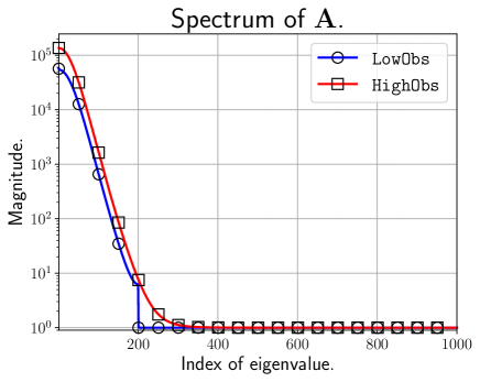
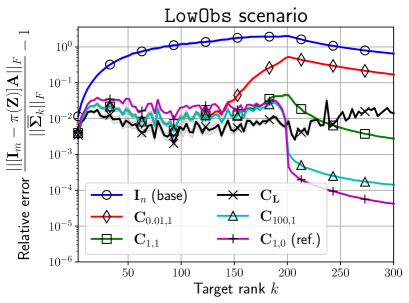
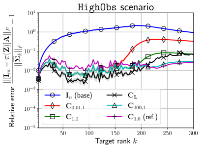
In our numerical experiments, we then aim to approximate the eigenspectrum of the symmetric positive definite matrix by using randomized SVD based on non-standard Gaussian sample matrices for the first Gauss-Newton iteration . For simplicity, we will use referring to . The error covariance matrix is obtained from the discretization of the diffusion operator on a regular grid, is chosen as a selection operator ( is a linear operator), and with being the standard deviation. The matrix of interest defined in (4.3) is a rank update of the identity. Consequently, the number of observations has a critical influence on the eigenvalue distribution, i.e. for there are eigenvalues equal to 1. The eigenvalues of also have a strongly decaying spectrum as shown in Figure 1 which is a property in favour of the randomized SVD. We choose , and we consider two different scenarios, with a different number of observations: LowObs for , and HighObs for .
4.1 Accuracy of the error bounds
In this section, we analyze the accuracy of the bounds in Theorem 3.1 for a particular choice of the covariance matrix . Note that the dominant eigenvectors of correspond to the dominant eigenvectors of , expressed as , with its rank equal to . Using the SVD, , where , and , the eigenspectrum of is then represented as . As a result, represents the eigenvectors of corresponding to the largest eigenvalues. Leveraging Theorem 3.1’s results, we can improve the performance of Algorithm 1 by choosing the covariance matrix , with being the target rank. Since is not readily available and is indeed the quantity of interest, we select . Note that is in the image of the matrix (this remark is further investigated in Section 4.2). When is an identity matrix, i.e. , . In the numerical experiments, is chosen as a selection operator. In this case, where is a submatrix of with its columns selected through the matrix . Therefore, the performance of Algorithm 1 will be improved with the choice of , whenever the subspace spanned by the -th leading eigenvectors of gets closer to the range of .
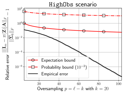
We apply Algorithm 1 with , being a matrix whose columns are independently drawn from a standard multivariate Gaussian distribution. We compare the bounds to the empirical mean of the randomized low-rank approximation error computed out of 20 independent runs of Algorithm 1. For the comparison, we plot the quantity
which is as close as zero as the low-rank approximation error is close to the optimal value . The coefficients and in Theorem 3.1 are obtained so that the probability of failure is strictly less than .
Figure 2 shows the low-rank approximation error with respect to the target rank , for a fixed oversampling parameter . Here, the bounds in expectation follow the empirical mean error trend, by a multiplicative factor of approximately . On Figure 2 (a) however, the bound diverges after . This behaviour illustrates that the use of in the covariance matrix may positively influence the low-rank approximation error as long as the target rank is smaller than . When , the algorithm is expected to produce approximations of eigenvectors associated with the cluster of eigenvalues at 1, which are no longer in the image of , thus explaining why the bound diverges. This problem is not noticeable in Figure 2 (b) since is equal to in this scenario and is at most 300. However, it is worth noting that the bounds diverge while the empirical error still decreases, highlighting that the bounds may overestimate the error in certain circumstances.
These considerations also apply to the probability bounds whose trends follow the expectation bounds. Given the small empirical standard deviation observed (grey halo around the empirical error), it is clear that the probability bounds severely overestimate the error by a factor of at least .
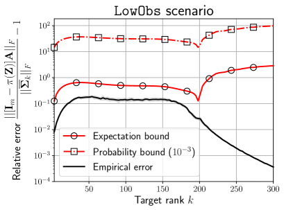
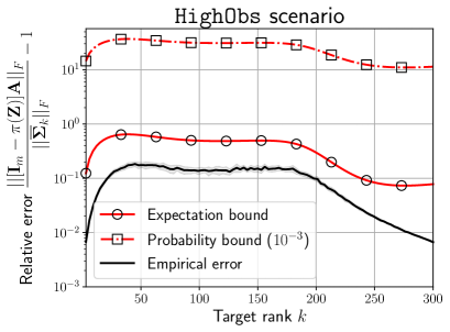
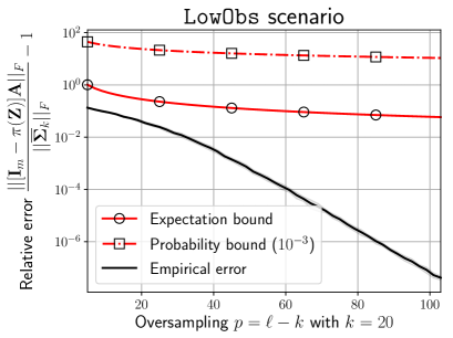
Figure 3 shows the behaviour of the bounds with respect to the oversampling parameter for a fixed value of the target rank (). We observe no significant differences between the LowObs and HighObs scenarios. The bounds in expectation and in probability both predict a decrease rate of the error as , but visibly fail to capture the true decrease rate.
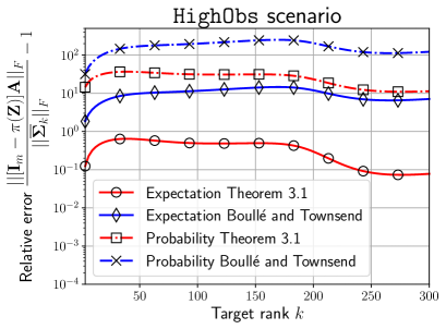
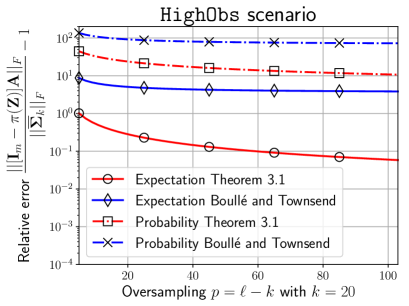
Finally, we propose in Figure 4 a comparison of the bounds from [1] in the HighObs scenario. This is meant to illustrate the discussion in Section 3.1.2, where we proposed alternative bounds to analyse the Generalized RSVD algorithm. We observe here that the bounds derived from Theorem 3.1 actually refine the ones from [1]. The impact of the extra factor can be seen in Figure 4 (a), where the refinement brought by Theorem 3.1 is greater for large values of : e.g. in expectation, the improvement is approximately equal to a factor of for small values of , and up to almost for larger values of . The decrease rate of the error with respect to the oversampling parameter, shown in Figure 4 (b), is also impacted.
4.2 Approximate subspace iteration
In this section, we consider in Algorithm 1 and we denote by the covariance matrix of which corresponds to . Our objective is to illustrate how Algorithm 1 behaves when is replaced by an approximation of in the power iteration. We note here that the power scheme applied to square matrices has the form of
| (4.4) |
where is a matrix whose columns are independently sampled from a standard multivariate Gaussian distribution. For our numerical experiments, we consider the following cases:
-
•
: This case corresponds to the exact power iteration with in Equation (4.4).
-
•
: This case corresponds to the exact power iteration with in Equation (4.4).
-
•
: This case can be interpreted as an approximate power iteration with , where is approximated by . Note that we assume .
-
•
: This case can be interpreted as an approximate power iteration with , where is approximated by .
The first case will serve as a reference, while the second one will serve as an ideal case. For the last two cases, we rely on the approximation that is an accurate approximation of . Ideally, if is an accurate enough approximation of , and a fortiori of , then the resulting low-rank approximation error should be close to the one obtained with in (4.4). In theory, it may even yield umproved performance since using is sub-optimal compared to .
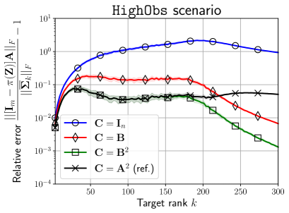
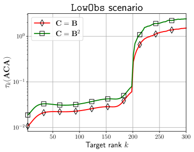
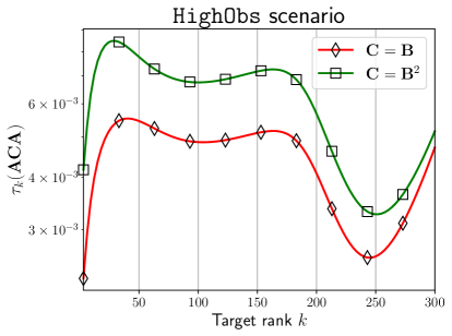
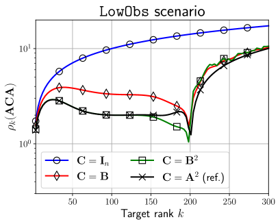
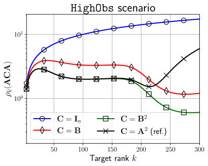
Figure 5 presents the numerical results for different cases. A first important observation is that for both scenarios, using or improves over the reference case , implying that corresponding covariance matrices are indeed carrying dominant eigeninformation of . Then, one also observes that applying Algorithm 1 with yields results very similar to and improved low-rank approximation for . These results suggest to use an approximation to instead of .
This is also what we observe when looking at the two parameters and shown in Figures 6 and 7, respectively. Let us recall that measures the stability of under the action of and that for in our case. From this, it is clear that is zero for the first two cases and is thus not shown in Figure 6. For the remaining two cases, we note that is relatively small compared to except in the LowObs scenario when . In this situation, the equality no longer holds, so the practical choice of using or instead of becomes less relevant. Nevertheless, this limitation should not have any practical limitations since in concrete applications, the target rank will be chosen much smaller than the number of observations. On the other side, is related to how the dominant eigenspectrum of approximates the one of . Likewise, for , we observe a significant increase after in the LowObs scenario. The explanation is similar, since after this point, the target low-rank approximation contains eigenmodes associated with the eigenvalue cluster at 1, while the chosen covariance matrix is only meant to improve the approximation of the first dominant eigenmodes.

4.3 Using available approximations
In this section, we study the case where approximations and of and respectively are already available. The objective here is to analyze the low-rank approximation error when using a covariance matrix of the specific form
For this numerical experiment, the approximations are obtained by applying Algorithm 1 to , with () and for varying values of target rank together with . Information on the quality of the resulting approximation is shown in Figure 5. We then use the resulting matrices and to construct the matrix . We study the following cases:
-
•
Different scaling: and for a fixed value . The scaling is expected to influence the performance as it allows to weight differently and its orthogonal complement.
-
•
For , we also consider the variant . Regarding the results from the previous subsection, using is expected to improve the performance.
-
•
We also consider the case and . As discussed in Section 3.1.3, this yields a deterministic algorithm which simply reduces to perform a standard power iteration step on top of . This choice will serve as a reference, and our objective is to study whether maintaining randomization (i.e. ) can yield better performance. This can be interpreted as the limit of when increases.
-
•
Finally, we consider the case corresponding to a single step of randomized power iteration. This base case is here to illustrate how using existing information actually improves performance.
The obtained results for the empirical low-rank approximation error are presented in Figure 8 and have been obtained from 20 independent applications of Algorithm 1.
Regardless of the scaling, for small values of (roughly ), the resulting low-rank approximation error is almost identical and also improves over the reference case. For larger , it seems that the larger is, the better the performance is. This suggests that in this situation, the approximation used to construct the covariance matrix is accurate enough to be trusted. Nevertheless, there is a trade-off to find since taking larger would asymptotically yield the same results as (the reference case). Finally, the most noticeable case is , which outperforms the reference case by almost a factor of 10 (given the target remains small enough). As expected, using allows us to improve the performance because also carries information. Of course, this also yields a more expensive algorithm since it would require an application of to a matrix, while the other scaled cases only involve thin matrices.
5 Conclusions
We have proposed a general theoretical framework for the analysis of the low-rank approximation error where we have relaxed the assumptions on the covariance matrix. The obtained bounds, in expectation and in probability, have clear interpretations. We have illustrated the generality of our result by applying Theorem 3.1 to two known algorithms, and the obtained bounds have comparable accuracy as the ones derived on purpose in the literature. Finally, we have illustrated our result on a data assimilation problem. First, we have studied the accuracy of the bounds. Then, we have proposed numerical experiments in two different situations, using either an approximation of or an available approximation of . In both cases, we have identified covariance matrices that enable us to improve the overall performance. This highlights that using the structure of the problem to design the covariance matrix does improve the performance of randomized low-rank approximation methods.
Appendix A Proof of Theorem 3.1
In this appendix, we prove Theorem 3.1. We begin with a lemma which is a generalization of the analysis in terms of principal angles proposed in [24].
Lemma A.1.
Let be an arbitrary matrix and a full column rank matrix such that . Let us denote and .
For any integer , if , then one has
| (A.1) |
where .
Proof.
By assumption, has full row rank and thus has a right multiplicative inverse . Hence satisfies the two relations
Moreover, we have which implies that according to [14, Proposition 8.5]. By using the conjugation rule (2.2) and the identity , we obtain
where the last equality is obtained using the Sherman-Morrison formula (2.4). To conclude, we observe that , which implies, using the conjugation rule (2.2), that . ∎
Remark. Let denote the principal angles between and , and the ones between and . The statement of Lemma A.1 can be geometrically rephrased as
Less formally, the forthcoming analysis is based on how close and are, while the truly computed error rather concerns how close is from . Since the latter is of dimension , while is of dimension , the looseness of the derived bounds will increase with .
The next result is a deterministic bound for the low-rank approximation error which generalizes [14, Proposition 9.6].
Proposition A.2 (Deterministic analysis).
Let be an arbitrary matrix and a full column rank matrix such that . Let us further denote and .
For any integer , if , then one has
Proof.
Remark. In the particular case where , we observe that Proposition A.2, up to different notation conventions, generalizes [14, Proposition 9.6].
Proposition A.3 is the final and main result from which Theorem 3.1 can be deduced. It addresses the stochastic analysis of a particular quantity that plays a central role in our proof.
Proposition A.3.
Let be an arbitrary matrix, and a matrix whose columns are independently sampled from a multivariate Gaussian distribution with covariance matrix , such that . Let us further denote and .
For any integer , if is non-singular, one has
Moreover, if , then for all one has
holds with probability at least .
Proof.
Expectation.
Using the theorem of total expectation one has
We consider the following partitioning
In the inner expectation, is a fixed matrix, but unlike the standard result in [14], and are not statistically independent. This implies that conditioned by , the columns of no longer follow a standard multivariate Gaussian distribution. Instead, if denotes the -th column of , then the -th column of follows a multivariate Gaussian distribution with mean term
and covariance matrix
Consequently, if one defines , one can write where the columns of are sampled from a standard Gaussian distribution. Thus, conditioned by one has
The linearity of the expectation allows us to deal with each term separately. Conditioned by , the first one is a non-random constant, and the second term can be handled using [14, Proposition 10.1] since has a standard multivariate Gaussian distribution. Concerning the third term, the linearity of the expectation conditioned by yields
Altogether, one has
where the last equality follows from the simplification of when substituting by its expression. Taking again the expectation yields
Since the columns of are independently sampled from a multivariate Gaussian distribution with zero mean and covariance matrix , the matrix follows a Wishart distribution of the form [20, Definition 3.1.3]. In addition, , where the second equality holds with probability one since . In fact, if is non-singular, the matrix is non-singular almost surely, see [20, Theorem 3.1.4]. In this case, according to [20, Theorem 3.2.12] for , one has
Hence, by the linearity of the expectation, one gets
which concludes the proof.
Probability.
Let . Using the reverse triangular inequality, it holds for any that
where the last inequality follows from the submultiplicativity property. Thus, is at worst -Lipschitz with . Applying [14, Proposition 10.3] then yields that if is a matrix whose columns are sampled from a standard Gaussian distribution, then one has
Hölder’s inequality yields , and combining this fact with the result proved right above and the properties of multivariate Gaussian distribution one has
Altogether, this implies that
| (A.2) |
Let us now consider, for , the event
Applying [1, Lemma 8] yields for all that
where denotes the complement of the event set . Now, by denoting the event considered in (A.2), the law of total probabilities reads
Since one trivially has and , one gets
or equivalently,
which ends the proof for the bound in probability.
Rearranging the terms.
It remains to transform the terms to get more interpretable bounds. Since by definition is orthogonal, and is full column rank, then using (2.5), one readily has
Then, using classical algebraic manipulations, one gets
The second term is trivially equal to , which finally yields
∎
Proof of Theorem 3.1: Bound in expectation
If is a matrix whose columns are independently sampled from a multivariate Gaussian distribution with covariance matrix , then has full row rank with probability 1. Hence, since the expectation is monotonic and linear, taking the expectation over in Proposition A.2 yields
Applying Proposition A.3 yields
so that we obtain
Using Hölder’s inequality, that is for any random variable , concludes the proof.
Proof of Theorem 3.1: Bound in probability
References
- [1] Nicolas Boullé and Alex Townsend. A generalization of the randomized singular value decomposition. arXiv:2105.13052 [cs, math, stat], January 2022.
- [2] Nicolas Boullé and Alex Townsend. Learning Elliptic Partial Differential Equations with Randomized Linear Algebra. Foundations of Computational Mathematics, 23:709–739, 2023.
- [3] N. Bousserez and Daven K. Henze. Optimal and scalable methods to approximate the solutions of large-scale Bayesian problems: Theory and application to atmospheric inversion and data assimilation. Quarterly Journal of the Royal Meteorological Society, 144(711):365–390, January 2018.
- [4] Nicolas Bousserez, Jonathan J. Guerrette, and Daven K. Henze. Enhanced parallelization of the incremental 4D-Var data assimilation algorithm using the Randomized Incremental Optimal Technique. Quarterly Journal of the Royal Meteorological Society, 146(728):1351–1371, April 2020.
- [5] Roger Daley. Atmospheric Data Analysis. Number 2 in Cambridge Atmospheric and Space Science Series. Cambridge University Press, Cambridge, first edition, 1999.
- [6] Ieva Daužickaitė, Amos S. Lawless, Jennifer A. Scott, and Peter Jan Leeuwen. Randomised preconditioning for the forcing formulation of weak-constraint 4D-Var. Quarterly Journal of the Royal Meteorological Society, 147(740):3719–3734, October 2021.
- [7] Carl Eckart and Gale Young. The approximation of one matrix by another of lower rank. Psychometrika, 1(3):211–218, September 1936.
- [8] Gene H. Golub and Charles F. Van Loan. Matrix Computations. Johns Hopkins Studies in the Mathematical Sciences. The Johns Hopkins University Press, Baltimore, fourth edition, 2013.
- [9] Gene Howard Golub and Charles F. Van Loan. Matrix Computations. Johns Hopkins Series in the Mathematical Sciences. Johns Hopkins university press, Baltimore London, third edition, 1996.
- [10] S. Gratton, A. S. Lawless, and N. K. Nichols. Approximate Gauss–Newton Methods for Nonlinear Least Squares Problems. SIAM Journal on Optimization, 18(1):106–132, January 2007.
- [11] S. Gratton, A. Sartenaer, and J. Tshimanga. On A Class of Limited Memory Preconditioners For Large Scale Linear Systems With Multiple Right-Hand Sides. SIAM Journal on Optimization, 21(3):912–935, July 2011.
- [12] Ming Gu. Subspace Iteration Randomization and Singular Value Problems. SIAM Journal on Scientific Computing, 37(3):A1139–A1173, January 2015.
- [13] Wolfgang Hackbusch. Hierarchical Matrices: Algorithms and Analysis. Number 49 in Hierarchical Matrices. Springer Berlin Heidelberg, Berlin, Heidelberg, first edition, 2015.
- [14] Nathan Halko, Per-Gunnar Martinsson, and Joel A. Tropp. Finding Structure with Randomness: Probabilistic Algorithms for Constructing Approximate Matrix Decompositions. SIAM Review, 53(2):217–288, January 2011.
- [15] Nicholas J. Higham. Functions of Matrices: Theory and Computation. Society for Industrial and Applied Mathematics, Philadelphia, 2008.
- [16] Roger A. Horn and Charles R. Johnson. Matrix Analysis. Cambridge University Press, Cambridge ; New York, second edition, 2012.
- [17] Andrew V. Knyazev and Merico E. Argentati. Principal Angles between Subspaces in an A-Based Scalar Product: Algorithms and Perturbation Estimates. SIAM Journal on Scientific Computing, 23(6):2008–2040, January 2002.
- [18] William Lahoz, Boris Khattatov, and Richard Menard, editors. Data Assimilation. Springer Berlin Heidelberg, Berlin, Heidelberg, 2010.
- [19] Michael W. Mahoney. Randomized Algorithms for Matrices and Data. Foundations and Trends® in Machine Learning, 3(2):123–224, 2010.
- [20] Robb J. Muirhead. Aspects of Multivariate Statistical Theory. Wiley Series in Probability and Mathematical Statistics. Wiley, New York, 1982.
- [21] Cameron Musco and Christopher Musco. Randomized Block Krylov Methods for Stronger and Faster Approximate Singular Value Decomposition. MIT Press, 1:1396–1404, October 2015.
- [22] Christopher C. Paige and M. Wei. History and generality of the CS decomposition. Linear Algebra and its Applications, 208–209:303–326, September 1994.
- [23] Vladimir Rokhlin, Arthur Szlam, and Mark Tygert. A Randomized Algorithm for Principal Component Analysis. SIAM Journal on Matrix Analysis and Applications, 31(3):1100–1124, January 2010.
- [24] Arvind K. Saibaba. Randomized Subspace Iteration: Analysis of Canonical Angles and Unitarily Invariant Norms. SIAM Journal on Matrix Analysis and Applications, 40(1):23–48, January 2019.
- [25] Arvind K. Saibaba, Joseph Hart, and Bart van Bloemen Waanders. Randomized algorithms for generalized singular value decomposition with application to sensitivity analysis. Numerical Linear Algebra with Applications, 28(4), August 2021.
- [26] Arvind K. Saibaba, Jonghyun Lee, and Peter K. Kitanidis. Randomized algorithms for generalized Hermitian eigenvalue problems with application to computing Karhunen–Loève expansion. Numerical Linear Algebra with Applications, 23(2):314–339, March 2016.
- [27] Alexandre Scotto Di perrotolo,. Randomized Numerical Linear Algebra Methods with Applications to Data Assimilation. PhD thesis, Toulouse, ISAE-SUPERO, September 2022.
- [28] Joel A. Tropp. Randomized block Krylov methods for approximating extreme eigenvalues. Numerische Mathematik, 150(1):217–255, January 2022.
- [29] Charles F. Van Loan. Generalizing the Singular Value Decomposition. SIAM Journal on Numerical Analysis, 13(1):76–83, March 1976.
- [30] Franco Woolfe, Edo Liberty, Vladimir Rokhlin, and Mark Tygert. A fast randomized algorithm for the approximation of matrices. Applied and Computational Harmonic Analysis, 25(3):335–366, November 2008.
- [31] Qiaochu Yuan, Ming Gu, and Bo Li. Superlinear Convergence of Randomized Block Lanczos Algorithm. In 2018 IEEE International Conference on Data Mining (ICDM), pages 1404–1409, Singapore, November 2018. IEEE.
- [32] Peizhen Zhu and Andrew V. Knyazev. Angles between subspaces and their tangents. Journal of Numerical Mathematics, 21(4):325–340, January 2013.