Practical and Scalable Quantum Reservoir Computing

Abstract

Quantum Reservoir Computing leverages quantum systems to solve complex computational tasks with unprecedented efficiency and reduced energy consumption. This paper presents a novel QRC framework utilizing a quantum optical reservoir composed of two-level atoms within a single-mode optical cavity. Employing the Jaynes-Cummings and Tavis-Cummings models, we introduce a scalable and practically measurable reservoir that outperforms traditional classical reservoir computing in both memory retention and nonlinear data processing. We evaluate the reservoir’s performance through two primary tasks: the prediction of time-series data via the Mackey-Glass task and the classification of sine-square waveforms. Our results demonstrate significant enhancements in performance with increased numbers of atoms, supported by non-destructive, continuous quantum measurements and polynomial regression techniques. This study confirms the potential of QRC to offer a scalable and efficient solution for advanced computational challenges, marking a significant step forward in the integration of quantum physics with machine learning technology.

I Introduction

Quantum reservoir computing (QRC) has emerged as a groundbreaking machine learning framework for temporal information processing (i.e., processing of time series) that is capable of addressing intricate tasks with remarkable efficiency and minimal energy consumption Fujii2017 ; chen2019learning ; CNY20 ; Dudas2023 ; Govia2021 ; Bravo2022 ; Hulser2023 ; Nokkala2021 ; Pena2021 ; Xia2022 ; Mujal2023 ; Fry2023 ; Kalfus2022 ; Yasuda23 ; Beni2023 ; Markovic2019 ; Lin2020 . There are also static “variants" of QRC that process vectors or single quantum states rather a time series, which should properly be referred to as quantum random kitchen sinks or quantum extreme learning machines Innocenti23 , for instance, Ghosh2019 ; Ghosh2021 ; Domingo2022 . The tasks addressed by QRC fall into two main categories: classical tasks that require quantum memories for processing nonlinear functions and datasets Fujii2017 ; Dudas2023 ; Govia2021 , and quantum tasks focused on recognizing quantum entanglements Ghosh2019 , measuring dispersive currents Angelatos2021 , and predicting molecule structures Domingo2022 . Of these categories, classical tasks provide a clearer basis for comparing the performance of QRC against classical reservoir computing (CRC) Tanaka2019 ; Appeltant2011 ; Pathak2018 ; Angelatos2021 ; Chen2022 ; Gauthier2021 .

Proposals for implementing quantum reservoirs have been advanced using various platforms, including coupled networks of qubits Fujii2017 ; chen2019learning ; CNY20 ; Domingo2022 ; Ghosh2021 ; Pena2021 ; Xia2022 ; Yasuda23 , fermions Ghosh2019 , harmonic oscillators Nokkala2021 , Kerr nonlinear oscillators Angelatos2021 , Rydberg atoms Bravo2022 , and optical pulses Beni2023 . Increasing the number of physical sites, such as qubits, oscillators, or atoms, within a quantum network can dramatically expand the Hilbert space by exponentially increasing the number of quantum basis states. Each of these basis states functions as a node within the quantum neural network, mirroring the role of a node in a classical neural network Fujii2017 or an optical neural network Wang2022 ; ma2023 . The exponential scalability of the basis states involved in computation underlies the advantage of QRC over CRC, with quantum phase transitions further enhancing the performance Pena2021 ; Xia2022 . However, the proposed implementations discussed above face challenges in scalability due to the considerable difficulty in establishing connections between each new site and all existing sites in a quantum network. Particularly, the readouts of information from quantum reservoirs have been proposed through various methods, including measuring probabilities on quantum basis states Dudas2023 , excitations of qubits Fujii2017 , occupations on lattice sites Ghosh2019 , and energies of oscillators Angelatos2021 . However, employing these conventional measurement techniques poses a significant hurdle to data processing efficiency. These methods often necessitate quantum tomography, which costs the complete destruction of the quantum reservoir to acquire readouts at each time step. Consequently, they demand a substantial number of repeated time evolutions, resulting in a considerable overhead.

In this paper, we present a quantum reservoir that offers both convenient scalability and practical measurability, achieved through the coupling of atoms and photons in an optical cavity. To assess its computing prowess, we evaluate its performance on two classical tasks: the Mackey-Glass task Fujii2017 , which demands long-term memory for predicting the future trend of an input function, and the sine-square waveform classification task Dudas2023 ; Markovic2019 , which requires nonlinearity of the reservoir to capture sudden, high-frequency shifts in a linearly inseparable input dataset. These classical inputs are embedded in the coherent driving of the cavity photon field, enabling the performance comparison between QRC and CRC.

Our quantum reservoir is more conveniently scalable compared to prior proposals, since newly added atoms automatically couple with the existing atoms through their mutual connections with the cavity photon field. The performance improvement associated with this scalability is evidenced by the diminishing gap between the actual and target outputs as the number of atoms increases. Practical readouts are obtained through a continuous quantum measurement, where the cavity field provides two readouts linked to two photonic quadratures, and each atom provides two readouts linked to two atomic spin channels Wiseman2010 ; BvHJ07 ; Wei2008 ; Ruskov2010 ; Hacohen2016 ; Ochoa2018 ; Fuchs2001 . In contrast to the tomography measurements in the prior methods, our continuous measurement scheme is considered non-destructive while its back-action on the reservoir is fully incorporated into our model. The exponential scaling of basis states underlying the limited number of observable readouts still plays an important role of making the system dynamics more nonlinear and more complex, ensuring the excellent performance of QRC.

II Results

II.1 Quantum Optical Reservoir

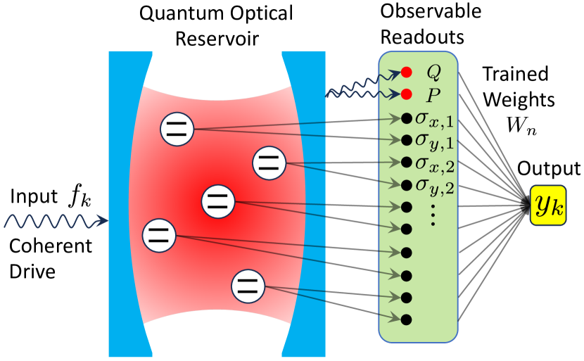
Figure 1: Setup of quantum optical reservoir computing. The reservoir is composed of atoms inside an optical cavity, exhibiting diverse detunings and couplings across various spatial positions. The input function is integrated into the coherent driving of the cavity. Readouts are obtained via continuous measurements of photonic quadratures and atomic spin channels. A machine learning process is employed to train the mapping from the readouts to the output.

The components of quantum reservoir computing include the input, the quantum reservoir, the readouts, and the output, as illustrated in Fig. 1. We employ a quantum optical system encompassing two-level atoms inside a single-mode optical cavity as the quantum reservoir. In the literature, this system is commonly known as the Jaynes-Cummings model for a single atom Jaynes1963 and the Tavis-Cummings model for multiple atoms Tavis1968 . The time-independent part of the Hamiltonian is expressed as

$$H_{0}=\omega_{c}c^{\dagger}c+\underset{i}{\sum}\omega_{i}\sigma_{i}^{\dagger}\sigma_{i}+\underset{i}{\sum}g_{i}\left(c^{\dagger}\sigma_{i}+c\sigma_{i}^{\dagger}\right),$$ (1)

where $c$ represents the photon annihilation operator, $\sigma_{i}=\left|g\right\rangle\left\langle e\right|_{i}$ denotes the lowering operator of the $i$-th atom with $\left|g\right\rangle$ ($\left|e\right\rangle$) representing the ground (excited) state, $\omega_{c}$ ($\omega_{i}$) describes the detuning between the coherent driving and the cavity (atomic) frequencies, and $g_{i}$ is the electric-dipole coupling strength between the $i$-th atom and the cavity mode. For QRC, it is essential to select either various detuning $\omega_{i}$ or various coupling strength $g_{i}$ to prompt the atoms to produce non-identical memories, thus enhancing their overall capability. This model can be practically implemented using cold atoms in an optical cavity Brennecke2007 ; Niemczyk2010 , where optical tweezers can be used to trap and measure individual atoms at different positions Kaufman2021 ; Ye2023 . Alternatively, quantum dots can also be utilized to induce random positioning, detuning, and coupling Schmidt2007 . The input function, denoted as $f\left(t\right)$, is integrated into the time-dependent coherent driving term

$$H_{1}\left(t\right)=i\epsilon f\left(t\right)\left(c-c^{\dagger}\right),$$ (2)

where $\epsilon$ is the driving strength.

The readouts from the quantum optical reservoir are determined through continuous quantum measurement, as elaborated in the “Methods” section. In the ideal scenario where the number of measurements approaches infinity, the readouts, denoted as $x_{n}\left(t\right)$, are directly correlated with the expectation values of experimental observables. The observables of the cavity field stem from the homodyne detection of two orthogonal quadratures Wiseman2010 ; BvHJ07 ; Nurdin14

$$Q =c+c^{\dagger},$$ (3)

$$P =i\left(c-c^{\dagger}\right),$$

and the observables of the atomic spontaneous emission are associated with the Pauli operators Wiseman2001

$$\sigma_{x,i} =\sigma_{i}+\sigma_{i}^{\dagger},$$ (4)

$$\sigma_{y,i} =i\left(\sigma_{i}-\sigma_{i}^{\dagger}\right).$$

It has been demonstrated that these observables of the cavity and atoms can be simultaneously measured Wei2008 ; Ruskov2010 ; Hacohen2016 ; Ochoa2018 . To establish a linear regression for training and testing the reservoir computer, the relation between readouts and observables is constructed as $x_{1}\left(t\right)=\left\langle Q\right\rangle$, $x_{2}\left(t\right)=\left\langle P\right\rangle$, $x_{3}\left(t\right)=\left\langle\sigma_{x,1}\right\rangle$, $x_{4}\left(t\right)=\left\langle\sigma_{y,1}\right\rangle$, and so forth. This leads to $N_{readouts}=2N_{atom}+2$, with $N_{readouts}$ and $N_{atom}$ the number of readouts and atoms, respectively. To enhance performance, a polynomial regression is also employed by incorporating both the linear and all the quadratic terms of these expectation values into the readouts. This includes terms such as $\left\langle Q\right\rangle^{2}$and $\left\langle P\right\rangle$$\left\langle\sigma_{x,i}\right\rangle$, resulting in $N_{readouts}=2N_{atom}^{2}+7N_{atom}+5$. The expectation values are calculated using the density operator, $\rho\left(t\right)$, whose dynamics, averaged over an infinite number of measurements, is idealized as the deterministic master equation

$$\frac{d\rho}{dt}=-i\left[H_{0}+H_{1}\left(t\right),\rho\right]+2\mathcal{D}\left[\sqrt{\kappa_{c}}c\right]\rho+2\underset{i}{\sum}\mathcal{D}\left[\sqrt{\kappa_{i}}\sigma_{i}\right]\rho,$$ (5)

where the Lindblad superoperator is defined as

$$\mathcal{D}\left[a\right]\rho=a\rho a^{\dagger}-\frac{1}{2}\left(a^{\dagger}a\rho+\rho a^{\dagger}a\right)$$ (6)

for any collapse operator $a$. To roughly maintain a constant total decay rate $\kappa$ as $N_{atom}$ increases, the decay rate of the cavity or each atom is assumed to be $\kappa_{c\left(i\right)}=\kappa/\left(2N_{atom}+2\right)$. A higher $\kappa$ reduces the uncertainty in the readout measurement, commonly referred to a strong measurement, while a lower $\kappa$ corresponds to a weak measurement Fuchs2001 .

Time discretization is essential within the framework of quantum reservoir computing Fujii2017 . The discretized time is expressed as $t_{k}=k\Delta t$, where the integer $k$ denotes the time index and $\Delta t$ represents the time step. During the time interval from $t_{k-1}$ to $t_{k}$, the discretized input maintains a constant value $f_{k}=f\left(t_{k}\right)$, where $f\left(t_{k}\right)$ originates from Eq. (2). The discretized readouts are sampled at $t_{k}$ as $x_{kn}=x_{n}\left(t_{k}\right)$, where a constant bias term $x_{k0}=1$ is also introduced.

The relationship between the readouts and output is trained through a learning process. Let $\bar{y}_{k}$ represent the target output capturing some key features of the input $f_{k}$. The objective of training is to determine the readout weights $W_{n}$ in order to achieve the actual output

$$y_{k}=\underset{n}{\sum}x_{kn}W_{n},$$ (7)

such that the normalized root mean square error

$${\rm NRMSE}=\frac{1}{\bar{y}_{max}-\bar{y}_{min}}\sqrt{\frac{\underset{k}{\sum}\left(y_{k}-\bar{y}_{k}\right)^{2}}{L}}$$ (8)

is minimized, where $L$ is the number of time steps in the training period. The approach for this minimization is discussed in “Methods”. To test the performance of reservoir computing, newly generated $x_{kn}$ and $\bar{y}_{k}$ in the testing period, along with the trained weights $W_{n}$, are utilized to calculate the NRMSE.

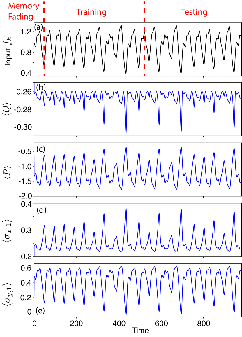
Figure 2: Input and readouts for the Mackey-Glass task. (a) The input function, $f_{k}$, divided into memory fading, training, and testing zones. (b)-(e) The corresponding readouts from a single-atom reservoir with $\omega_{1}=20$ and $g_{1}=30$. Parameters: $Delay=20$, $\kappa=10$, $\omega_{c}=40$, and $\epsilon=20$.

II.2 Mackey-Glass task

The Mackey-Glass task serves as a test for long-term memory, demanding the reservoir to retain past information from the input function to forecast its future behavior. The input function is generated from the Mackey-Glass equation

$$\frac{df\left(t\right)}{dt}=\frac{\beta f\left(t-\tau_{M}\right)}{1+f^{10}\left(t-\tau_{M}\right)}-\gamma f\left(t\right),$$ (9)

where the parameters $\beta=0.2$, $\gamma=0.1$, and $\tau_{M}=17$ are commonly accepted standard values in the chaotic regime Fujii2017 ; Dudas2023 ; Hulser2023 . We apply a buffer by discarding the first $1000$ time units in Eq. (9), thus considering the discretized function $f_{k}=f\left(t+1000\right)$ as the actual input, with discretized time $t=kdt$, as depicted in Figure 2(a). The time series is sampled with a time step of $dt=1$. The target output, $\bar{y}_{k}$, predicting the future of the input function with a time $Delay$, is constructed as $\bar{y}_{k}=f_{k+Delay}$.

The proposed quantum optical reservoir is highly compatible with the Mackey-Glass task, as it exhibits discernible responses to various input waveforms, which are quantified by the readouts of observables illustrated in Figure 2(b)-(e). The time period for the simulation is divided into three intervals for the purposes of memory fading, training and testing. The memory fading phase guarantees that during training and testing, the readouts depend solely on the input function rather than the initial state of the master equation.

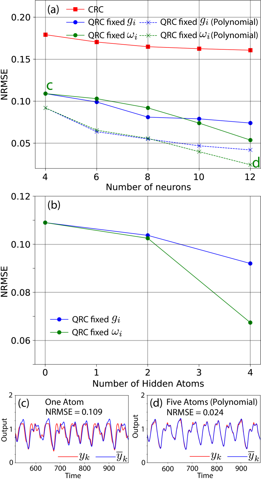
Figure 3: Testing result for the Mackey-Glass task with various reservoir scales. (a) NRMSE plotted against the number of neurons, where readouts are obtained from all neurons. Blue lines: fixed $g_{i}=30$ for all atoms and $\omega_{i}=20$ for one atom, $\omega_{i}=[0,40]$ for two atoms, $\omega_{i}=[0,20,40]$ for three atoms, $\omega_{i}=[0,10,30,40]$ for four atoms, and $\omega_{i}=[0,10,20,30,40]$ for five atoms. Green lines: fixed $\omega_{i}=20$ for all atoms and $g_{i}=30$ for one atom, $g_{i}=[10,50]$ for two atoms, $g_{i}=[10,30,50]$ for three atoms, $g_{i}=[10,20,40,50]$ for four atoms, and $g_{i}=[10,20,30,40,50]$ for five atoms. Solid lines: regular linear regression. Dashed lines: polynomial regression incorporating both linear and quadratic terms of observables. Red line: CRC averaging $1000$ random trajectories on the echo state network. (b) NRMSE as a function of the number of hidden (unmeasured) atoms in QRC, while maintaining measurement of $4$ specified neurons from the cavity field and the particular atom (denoted as the 0-th atom) with $g_{0}=30$ and $\omega_{0}=20$. (c)-(d) Actual (red) and target (blue) outputs from QRC with one atom (linear regression) and five atoms (polynomial regression), corresponding to the points marked by letters “c” and “d” in panel (a), respectively. Parameters: $Delay=20$, $\kappa=10$, $\omega_{c}=40$, $\epsilon=20$.

Figure 3 illustrates the performance enhancement as the quantum reservoir scales up, demonstrating the scalability of QRC. The scale of QRC is determined by two factors: (i) the number of observables, which is determined by the number of channels one wishes to measure, with a maximum availability of $2N_{atom}+2$; and (ii) the number of basis states spanning the Hilbert space, which scales as $N_{c}2^{N_{atom}}$, with $N_{c}$ the number of involved photon Fock states. In QRC, the number of observables is also referred to as the number of neurons. The blue and green solid lines in Fig. 3(a) shows the decrease in NRMSE as the number of atoms increases from $1$ to $5$, where measurements of the cavity field and all atoms lead to a corresponding increase in the number of neurons from $4$ to $12$. For comparison, the red solid line in Fig. 3(a) shows the performance of CRC as a function of the number of neurons in an echo state network, with further details discussed in “Methods”. The advantage of QRC over CRC is attributed to the exponentially increasing number of quantum basis states underlying the few measured neurons. The power of increasing basis states is further demonstrated in Fig. 3(b), where the number of measured neurons is fixed at $4$ (including $2$ cavity and $2$ atomic observables), while additional hidden (unmeasured) atoms is introduced to expand the computational Hilbert space. The improved performance for a fixed number of measured output neurons with an increase in the dimension of the QRC Hilbert space has previously been observed for Ising models of QRC Fujii2017 ; chen2019learning . A possible reason for this could be that, for the particular tasks considered, more complex fading memory maps generated by the QRC as the Hilbert space is increased are able to better capture features in the task to be learned. However, the improvement is expected to eventually plateau for a high enough dimension of the Hilbert space.

The outcome from the polynomial regression, incorporating both linear and quadratic terms of all observables, is depicted by the dashed lines in Fig. 3(a). The result is consistent with previous research indicating that appending nonlinear readouts from a reservoir can notably enhance performance Araujo2020 ; Govia2021 . A comparison between two extreme cases, linear regression with one atom and polynomial regression with five atoms, is illustrated in Fig. 3(c)(d), demonstrating a substantial performance improvement resulting from the combination of scalability and polynomial regression.

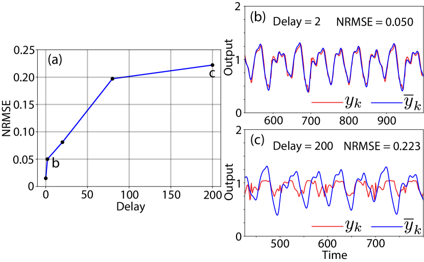
Figure 4: Testing result for the Mackey-Glass task with various $Delay$. (a) NRMSE as a function of $Delay$ for a three-atom QRC with $g=30$ and $\omega_{i}=[0,20,40]$. (b)(c) The actual (red) and target (blue) outputs with $Delay=2$ and $Delay=200$, corresponding to the points marked by letters “b” and “c” in panel (a), respectively. Parameters: $\kappa=10$, $\omega_{c}=40$, $\epsilon=20$.

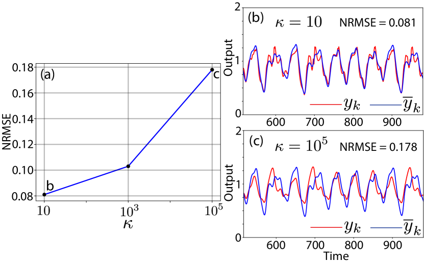
Figure 5: Testing result for the Mackey-Glass task with various decay rate $\kappa$. (a) NRMSE as a function of $\kappa$ for three-atom QRC with $g=30$ and $\omega_{i}=[0,20,40]$. (b)(c) The actual (red) and target (blue) outputs with $\kappa=10$ and $\kappa=10^{5}$, corresponding to the points marked by letters “b” and “c” in panel (a), respectively. Parameters: $Delay=20$, $\omega_{c}=40$, $\epsilon=20$.

The effects of $Delay$ and the decay rate $\kappa$ are shown in Figs. 4 and 5, respectively. As per Eq. (9), a longer $Delay$ necessitates a stronger memory for the reservoir to “remember” more past information from the input in order to forecast the future output, making the task increasingly challenging. Conversely, a larger $\kappa$ tends to cause the reservoir to “forget” input information more quickly due to photon leakage and atomic spontaneous emission. However, a larger $\kappa$ is beneficial for stronger measurements with reduced uncertainties in readouts. Therefore, selecting a balanced $\kappa$ will be crucial in experiments.

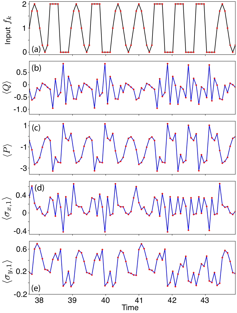
Figure 6: Input and readouts for the sine-square waveform classification task, where $110$ random waveforms are sent in as the input, with $10$ waveforms allocated for memory fading, $50$ waveforms for training, and $50$ waveforms for testing. (a) A segment of the input function, $f_{k}$, representing the first $10$ waveforms during the testing zone. (b)-(e) The corresponding readouts from a single-atom reservoir with $\omega_{1}=20$ and $g_{1}=30$. Parameters: $\omega_{c}=40$, $\kappa=10$, $\epsilon=20$, $\omega_{ss}=10$, $N_{ss}=8$.

II.3 Sine-square waveform classification task

The objective of the classification task is to determine whether each input data point belongs to a sine or a square waveform. The time-dependent input, $f_{k}$, comprises $110$ randomly generated sine and square waveforms. Among these, $10$ waveforms are allocated for memory fading, $50$ for training, and $50$ for testing. Each waveform is discretized into $N_{ss}$ points, leading to a time step of $\Delta t=2\pi/\left(N_{ss}\omega_{ss}\right)$, where $\omega_{ss}$ denotes the oscillation frequency of the input. Figure 6(a) depicts these discretized time points (red dots) across the first $10$ waveforms during the testing phase. The target output, $\bar{y}_{k}$, aimed at classifying the input signal, is set to $0$ if the input point belongs to a square waveform, and $1$ if it belongs to a sine waveform.

The sine-square waveform classification is a nonlinearity task that requires the reservoir to process a linearly inseparable input dataset containing abrupt changes. In a linear, closed quantum system, the smoothly evolving expectation values in readouts, $\left\langle c\right\rangle\propto\exp\left(-i\omega_{c}t\right)$ and $\left\langle\sigma_{i}\right\rangle\propto\exp\left(-i\omega_{i}t\right)$, are unable to capture these high-frequency, abrupt shifts. The introduction of nonlinearity, originating from the pumping and decay in the open quantum system, enhances the reservoir’s capability to promptly respond to the abrupt changes in the input. This is evidenced by the distinct readout measurements in Fig. 6(b)-(e), which correspond one-on-one to the input waveforms in Fig. 6(a).

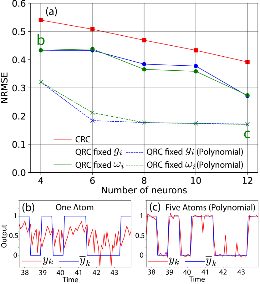
Figure 7: Testing result for the sine-square waveform classification task with various reservoir scales. (a) NRMSE plotted against the number of neurons, featuring results from QRC with linear regression, QRC with polynomial regression, and CRC on echo state network, where the parameters $\omega_{i}$ and $g_{i}$ align with those in Fig. 3. (b)(c) The actual (red) and target (blue) outputs from QRC with one atom (linear regression) and five atoms (polynomial regression), corresponding to the points marked by letters “b” and “c” in panel (a), respectively. Parameters: $\omega_{c}=40$, $\kappa=10$, $\epsilon=20$, $\omega_{ss}=10$, and $N_{ss}=8$.

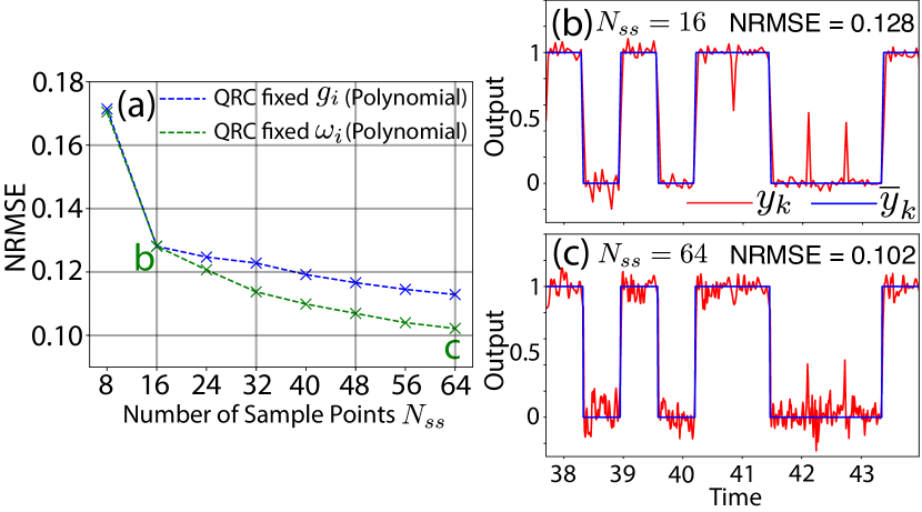
Figure 8: Testing result for the sine-square waveform classification task with various numbers of sample points, $N_{ss}$, within each period of the sine or square waveform. (a) NRMSE as a function of $N_{ss}$ for two sets of five-atom QRCs with $g_{i}=30$ and $\omega_{i}=[0,10,20,30,40]$ (blue) and with $\omega_{i}=20$ and $g_{i}=[10,20,30,40,50]$ (green), utilizing polynomial regression. The point at $N_{ss}=8$ corresponds to the "c" marker in Fig. 7(a). (b)(c) The actual (red) and target (blue) outputs with $N_{ss}=16$ and $N_{ss}=64$, corresponding to the "b" and "c" markers in panel (a), respectively. Parameters: $\omega_{c}=40$, $\kappa=10$, $\epsilon=20$, and $\omega_{ss}=10$.

The performance enhancements resulting from scalability and polynomial regression, along with the comparison between QRC and CRC, are shown in Fig. 7. It is observed that the performance associated with polynomial regression, represented by the blue and green dashed lines in Fig. 7(a), tends to saturate at $8$ neurons. This performance saturation suggests that the maximum performance achievable with the current sample size, associated with $N_{ss}=8$, has been attained. The corresponding comparison between the actual and target outputs is illustrated in Fig. 7(c), where discrepancies primarily occur at the first sample point in each waveform. Figure 8 shows that these discrepancies can be mitigated by increasing the number of sample points, $N_{ss}$, within each period of the sine or square waveform. This is evidenced by the decrease in NRMSE, as shown in Fig. 8(a). The comparison between Fig. 8(b) and Fig. 8(c) reveals that larger $N_{ss}$ reduces the impact of abrupt shifts in the input waveform on the output. Meanwhile, it also introduces more small oscillations resulting from higher-frequency changes in the input function due to smaller $\Delta t$.

III Discussion

We have introduced a paradigm for quantum optical reservoir computing with capabilities in quantum memory and nonlinear data processing. The inputs are classical functions integrated into the coefficient of coherent driving, allowing for direct comparison with the performance of classical reservoir computing. Notably, quantum decoherence of the reservoir facilitates the memory fading without the need for external erasing. This means that readouts are solely determined by the input, rather than by the initial state, after a certain period of quantum dissipation. Compared to other schemes of quantum reservoir computing, our paradigm has two major advantages: practicality and scalability.

In terms of practicality, continuous quantum measurement utilizing the homodyne detections of cavity quadratures and atomic spins is considered. These detections of non-commuting observables can be in fact carried out simultaneously Wei2008 ; Ruskov2010 ; Hacohen2016 ; Ochoa2018 and do not require tomography, making them more feasible than measurements of probability distributions in quantum basis states proposed in pervious works Fujii2017 ; Ghosh2019 ; Dudas2023 ; Angelatos2021 .

Our presented quantum optical reservoir offers convenient scalability compared to reservoirs built upon quantum networks, such as the Ising Fujii2017 and Fermi-Hubbard Ghosh2019 models. This is attributed to the coupling style between atoms and the single-mode cavity field. Specifically, to add a new atom, we only need to couple it with the cavity field, which will automatically induce its coupling with the rest of the atoms in the reservoir. Moreover, the number of quantum basis states in our reservoir scales proportionally to $2^{N_{atom}}$, enabling faster growth compared to the reservoirs not based on quantum networks, such as a single Kerr nonlinear oscillator Govia2021 and two coupled linear oscillators Dudas2023 . The increase in basis states, by itself, is able to improve the performance of QRC, as demonstrated by Fig. 3(b). This exponential scaling is also a crucial factor in the advantage demonstrated by the comparison between QRC and CRC, as shown in Figs. 3(a) and 7(a).

Additionally, previous studies have indicated that appending nonlinear post-processing to the readouts can enhance the performance of both QRC Govia2021 and CRC Paquot2012 ; Appeltant2011 ; Brunner2013 . In our work, this idea is implemented through polynomial regression, which additionally appends quadratic combinations of observable expectations to the readout matrix. The results demonstrate a significant improvement in performance.

IV Methods

IV.1 Continuous quantum measurement

Continuous quantum measurements are simulated for both the cavity field and individual atoms. For the cavity field, homodyne detection of two orthogonal quadratures involves splitting the system’s output beam into two using a beam-splitter, followed by homodyning each beam with the same local oscillator, differing by a phase shift of $\pi/2$ Wiseman2010 . Similarly, for atoms, homodyne detection is performed for spontaneous emissions Wiseman2001 . These measurements can be conducted concurrently Wei2008 ; Ruskov2010 ; Hacohen2016 ; Ochoa2018 . Consequently, the continuous measurement process is described by the stochastic master equation VPB79 ; VPB88 ; VPB91a ; HC93 ; Wiseman2010 ; BvHJ07 ; Nurdin14

$$d\rho_{J} =-i\left[H_{0}+H_{1}\left(t\right),\rho_{J}\right]dt$$ (10)

$$+2\mathcal{D}\left[\sqrt{\kappa_{c}}c\right]\rho_{J}dt+2\underset{i}{\sum}\mathcal{D}\left[\sqrt{\kappa_{i}}\sigma_{i}\right]\rho_{J}dt$$

$$+\left(dW_{Q}\mathcal{H}\left[\sqrt{\kappa_{c}}c\right]+dW_{P}\mathcal{H}\left[i\sqrt{\kappa_{c}}c\right]\right)\rho_{J}$$

$$+\underset{i}{\sum}\left(dW_{x,i}\mathcal{H}\left[\sqrt{\kappa_{i}}\sigma_{i}\right]+dW_{y,i}\mathcal{H}\left[i\sqrt{\kappa_{i}}\sigma_{i}\right]\right)\rho_{J},$$

where the deterministic part is governed by the Lindblad superoperator $\mathcal{D}$ defined in Eq. (6), and the stochastic part is determined by the superoperator $\mathcal{H}$ defined as

$$\mathcal{H}\left[a\right]\rho_{J}=a\rho_{J}+\rho_{J}a^{\dagger}-\left\langle a+a^{\dagger}\right\rangle_{J}\rho_{J}$$ (11)

for any stochastic collapse operator $a$. The continuous quantum measurements of the observables $Q$, $P$, $\sigma_{x,i}$, and $\sigma_{y,i}$ are associated with the stochastic collapse operators $\sqrt{\kappa_{c}}c$, $i\sqrt{\kappa_{c}}c$, $\sqrt{\kappa_{i}}\sigma_{i}$, and $i\sqrt{\kappa_{i}}\sigma_{i}$, respectively Wiseman2010 ; BvHJ07 ; Nurdin14 . The randomness of the measurement records is taken into account by the Wiener increments, $dW_{Q\left(P\right)}$ and $dW_{x\left(y\right),i}$, each of which selects a random number from a Gaussian probability distribution with a width of $dt$. The efficiencies of various detection channels are incorporated into the Wiener increments.

Each measurement detects the continuous currents in cavity and atom channels with noises, with the measurement records given by $\left\langle Q\left(P\right)\right\rangle_{J}+dW_{Q\left(P\right)}/dt$ and $\left\langle\sigma_{x\left(y\right),i}\right\rangle_{J}+dW_{x\left(y\right),i}/dt$, where the expectation values are computed using $\rho_{J}$ from Eq. (10). As the number of measurements approaches infinity, the impacts of the measurement back-actions, $dW_{Q\left(P\right)}$ and $dW_{x\left(y\right),i}$, are averaged out. This idealization is described by the deterministic master equation (5), accompanied by the averaged measurement records $\left\langle Q\left(P\right)\right\rangle$ and $\left\langle\sigma_{x\left(y\right),i}\right\rangle$, where the expectation values are computed using $\rho$.

IV.2 Minimization of NRMSE for training

The objective of training is to find the optimized weights $W_{n}$ that minimize the NRMSE defined in Eq. (8). Since ${\rm NRMSE^{2}}$, being a quadratic function of $W_{n}$, only has a global minimum but no local minima, a pseudoinverse method is sufficient for minimization. The readouts, $x_{kn}$, along with the constant bias term $x_{k0}=1$, are arranged in an $L\times\left(N_{readouts}+1\right)$ matrix ${\bf X}$, where $L$ is the number of time steps for training. The target output, $\bar{y}_{k}$, is organized in an $L\times 1$ column vector ${\bf{\bf\bar{Y}}}$. The weights, $W_{n}$, are arranged in a $\left(N_{readouts}+1\right)\times 1$ column vector ${\bf W}$. The optimized weight ${\bf{\bf W}}$ that minimizes NRMSE is therefore determined by Dion2018 ; Govia2021

$${\bf W}={\bf X}^{+}{\bf\bar{Y}},$$ (12)

where the Moore-Penrose pseudoinverse

$${\bf X}^{+}=\left({\bf X^{{\rm T}}}{\bf X}+\delta{\bf I}\right)^{-1}{\bf X^{{\rm T}}},$$ (13)

with ${\bf I}$ being the identity square matrix, and $\delta=10^{-10}$ is a ridge-regression parameter used to prevent overfitting.

IV.3 Classical reservoir computing

For the classical reservoir computing results, we use echo state networks (ESNs) described by

$${\bf x}_{k_{1}} ={\rm ReLU}({\bf Ax}_{k}+{\bf B}u_{k})$$ (14)

$$y_{k} ={\bf W^{\rm T}x}_{k}+C,$$ (15)

where $x_{k}$ is the vector-valued readout of the ESN at time step $k$ with length $N_{readouts}$, $u_{k}$ is the input, ${\bf W}$ and $C$ are fitting parameters obtained through optimization, and $y_{k}$ is the output at $k$. The activation function we use is the rectified linear unit ${\rm ReLU}(z)=\max(0,z)$ for a scalar $z$, and for vector arguments ${\bf x}$ the function is applied to each element of the vector so that $({\rm ReLU}({\bf x}))_{i}={\rm ReLU}(x_{i})=\max(0,x_{i})$. An individual ESN is defined by the choice of the matrix ${\bf A}$ and the vector ${\bf B}$.

In the results of Figs. 3(a) and 7(a), we get an average over $1000$ ESNs by choosing ${\bf A}$ and ${\bf B}$ randomly, with the constraint that that largest singular value of ${\bf A}$ must be less that 1 to ensure convergence. The number of neurons in these figures corresponds to the vector length of ${\bf x}_{k}$ (and therefore ${\bf W}$) given by $N_{readouts}$. Training of ${\bf W}$ and $C$ is performed using linear regression described in Section IV.2 by extending ${\bf W}$ to an $(N_{readouts}+1)$-dimensional vector with $W_{0}=C$.

References

- (1) K. Fujii and K. Nakajima, Phys. Rev. Appl. 8, 024030 (2017).
- (2) J. Chen and H. I. Nurdin, Quantum Information Processing 18, 198 (2019).
- (3) J. Chen, H. I. Nurdin, and N. Yamamoto, Phys. Rev. Applied 14, 024065 (2020).
- (4) J. Dudas, B. Carles, E. Plouet, F. A. Mizrahi, J. Grollier, and D. Marković, npj Quantum Information 9, 64 (2023).
- (5) L. C. G. Govia, G. J. Ribeill, G. E. Rowlands, H. K. Krovi, and T. A. Ohki, Phys. Rev. Res. 3, 013077 (2021).
- (6) R. A. Bravo, K. Najafi, X. Gao, and S. F. Yelin, PRX Quantum 3, 030325 (2022).
- (7) T. Hülser, F. Köster, K. Lüdge, and L. Jaurigue, Nanophotonics 12, 937 (2023).
- (8) J. Nokkala, R. Martínez-Peña, G. L. Giorgi, V. Parigi, M. C. Soriano, and R. Zambrini, Communications Physics 4, 53 (2021).
- (9) R. Martínez-Peña, G. L. Giorgi, J. Nokkala, M. C. Soriano, and R. Zambrini, Phys. Rev. Lett. 127, 100502 (2021).
- (10) W. Xia, J. Zou, X. Qiu, and X. Li, Frontiers of Physics 17, 33506 (2022).
- (11) P. Mujal, R. Martínez-Peña, G. L. Giorgi, M. C. Soriano, and R. Zambrini, npj Quantum Information 9, 16 (2023).
- (12) D. Fry, A. Deshmukh, S. Y.-C. Chen, V. Rastunkov, and V. Markov, Scientific Reports 13, 19326 (2023).
- (13) W. D. Kalfus, G. J. Ribeill, G. E. Rowlands, H. K. Krovi, T. A. Ohki, and L. C. G. Govia, Phys. Rev. Res. 4, 033007 (2022).
- (14) T. Yasuda et al., arXiv preprint arXiv:2310.06706 (unpublished).
- (15) J. García-Beni, G. L. Giorgi, M. C. Soriano, and R. Zambrini, Phys. Rev. Appl. 20, 014051 (2023).
- (16) D. Marković, N. Leroux, M. Riou, F. Abreu Araujo, J. Torrejon, D. Querlioz, A. Fukushima, S. Yuasa, J. Trastoy, P. Bortolotti, and J. Grollier, Applied Physics Letters 114, 012409 (2019).
- (17) J. Lin, Z. Y. Lai, and X. Li, Phys. Rev. A 101, 052327 (2020).
- (18) L. Innocenti et al., Commun. Phys. 6, 118 (2023).
- (19) S. Ghosh, A. Opala, M. Matuszewski, T. Paterek, and T. C. H. Liew, npj Quantum Information 5, 35 (2019).
- (20) S. Ghosh, T. Krisnanda, T. Paterek, and T. C. H. Liew, Communications Physics 4, 105 (2021).
- (21) L. Domingo, G. Carlo, and F. Borondo, Phys. Rev. E 106, L043301 (2022).
- (22) G. Angelatos, S. A. Khan, and H. E. Türeci, Phys. Rev. X 11, 041062 (2021).
- (23) G. Tanaka, T. Yamane, J. B. Héroux, R. Nakane, N. Kanazawa, S. Takeda, H. Numata, D. Nakano, and A. Hirose, Neural Networks 115, 100 (2019).
- (24) L. Appeltant, M. C. Soriano, G. Van der Sande, J. Danckaert, S. Massar, J. Dambre, B. Schrauwen, C. R. Mirasso, and I. Fischer, Nature Communications 2, 468 (2011).
- (25) J. Pathak, B. Hunt, M. Girvan, Z. Lu, and E. Ott, Phys. Rev. Lett. 120, 024102 (2018).
- (26) X. Chen, F. A. Araujo, M. Riou, J. Torrejon, D. Ravelosona, W. Kang, W. Zhao, J. Grollier, and D. Querlioz, Nature Communications 13, 1016 (2022).
- (27) D. J. Gauthier, E. Bollt, A. Griffith, and W. A. S. Barbosa, Nature Communications 12, 5564 (2021).
- (28) T. Wang, S.-Y. Ma, L. G. Wright, T. Onodera, B. C. Richard, and P. L. McMahon, Nature Communications 13, 123 (2022).
- (29) S.-Y. Ma, T. Wang, J. Laydevant, L. G. Wright, and P. L. McMahon, Quantum-noise-limited optical neural networks operating at a few quanta per activation, 2023.
- (30) H. M. Wiseman and G. J. Milburn, Quantum Measurement and Control (Cambridge University Press, Cambridge, 2009).
- (31) L. Bouten, R. van Handel, and M. R. James, SIAM J. Control Optim. 46, 2199 (2007).
- (32) H. Wei and Y. V. Nazarov, Phys. Rev. B 78, 045308 (2008).
- (33) R. Ruskov, A. N. Korotkov, and K. Mølmer, Phys. Rev. Lett. 105, 100506 (2010).
- (34) S. Hacohen-Gourgy, L. S. Martin, E. Flurin, V. V. Ramasesh, K. B. Whaley, and I. Siddiqi, Nature 538, 491 (2016).
- (35) M. A. Ochoa, W. Belzig, and A. Nitzan, Scientific Reports 8, 15781 (2018).
- (36) C. A. Fuchs and K. Jacobs, Phys. Rev. A 63, 062305 (2001).
- (37) E. Jaynes and F. Cummings, Proceedings of the IEEE 51, 89 (1963).
- (38) M. Tavis and F. W. Cummings, Phys. Rev. 170, 379 (1968).
- (39) F. Brennecke, T. Donner, S. Ritter, T. Bourdel, M. Köhl, and T. Esslinger, Nature 450, 268 (2007).
- (40) T. Niemczyk, F. Deppe, H. Huebl, E. P. Menzel, F. Hocke, M. J. Schwarz, J. J. Garcia-Ripoll, D. Zueco, T. Hümmer, E. Solano, A. Marx, and R. Gross, Nature Physics 6, 772 (2010).
- (41) A. M. Kaufman and K.-K. Ni, Nature Physics 17, 1324 (2021).
- (42) M. Ye, Y. Tian, J. Lin, Y. Luo, J. You, J. Hu, W. Zhang, W. Chen, and X. Li, Phys. Rev. Lett. 131, 103601 (2023).
- (43) N. N. Ledentsov, V. A. Shchukin, M. Grundmann, N. Kirstaedter, J. Böhrer, O. Schmidt, D. Bimberg, V. M. Ustinov, A. Y. Egorov, A. E. Zhukov, P. S. Kop’ev, S. V. Zaitsev, N. Y. Gordeev, Z. I. Alferov, A. I. Borovkov, A. O. Kosogov, S. S. Ruvimov, P. Werner, U. Gösele, and J. Heydenreich, Phys. Rev. B 54, 8743 (1996).
- (44) H. I. Nurdin, Russian J. Math. Phys 21, 386 (2014).
- (45) H. M. Wiseman and L. Diósi, Chemical Physics 268, 91 (2001).
- (46) F. Abreu Araujo, M. Riou, J. Torrejon, S. Tsunegi, D. Querlioz, K. Yakushiji, A. Fukushima, H. Kubota, S. Yuasa, M. D. Stiles, and J. Grollier, Scientific Reports 10, 328 (2020).
- (47) Y. Paquot, F. Duport, A. Smerieri, J. Dambre, B. Schrauwen, M. Haelterman, and S. Massar, Scientific Reports 2, 287 (2012).
- (48) D. Brunner, M. C. Soriano, C. R. Mirasso, and I. Fischer, Nature Communications 4, 1364 (2013).
- (49) V. P. Belavkin, preprint 411, Institute of Physics, Nicolaus Copernicus University, Torun (unpublished).
- (50) V. P. Belavkin, in Modelling and Control of Systems in Engineering, Quantum Mechanics, Economics, and Biosciences, edited by A. Blaquiere (Springer Verlag, New York, 1988), pp. 245–265.
- (51) V. P. Belavkin, in Quantum Aspects of Optical Communication, Vol. 45 of Lecture Notes in Physics (Springer, Berlin, 1991), pp. 151–163.
- (52) H. Carmichael, An Open Systems Approach to Quantum Optics (Springer, Berlin, 1993).
- (53) G. Dion, S. Mejaouri, and J. Sylvestre, Journal of Applied Physics 124, 152132 (2018).