Variational Schrödinger Diffusion Models

Abstract

Schrödinger bridge (SB) has emerged as the go-to method for optimizing transportation plans in diffusion models. However, SB requires estimating the intractable forward score functions, inevitably resulting in the costly implicit training loss based on simulated trajectories. To improve the scalability while preserving efficient transportation plans, we leverage variational inference to linearize the forward score functions (variational scores) of SB and restore simulation-free properties in training backward scores. We propose the variational Schrödinger diffusion model (VSDM), where the forward process is a multivariate diffusion and the variational scores are adaptively optimized for efficient transport. Theoretically, we use stochastic approximation to prove the convergence of the variational scores and show the convergence of the adaptively generated samples based on the optimal variational scores. Empirically, we test the algorithm in simulated examples and observe that VSDM is efficient in generations of anisotropic shapes and yields straighter sample trajectories compared to the single-variate diffusion. We also verify the scalability of the algorithm in real-world data and achieve competitive unconditional generation performance in CIFAR10 and conditional generation in time series modeling. Notably, VSDM no longer depends on warm-up initializations and has become tuning-friendly in training large-scale experiments.

1 Introduction

Diffusion models have showcased remarkable proficiency across diverse domains, spanning large-scale generations of image, video, and audio, conditional text-to-image tasks, and adversarial defenses (Dhariwal & Nichol, 2022; Ho et al., 2022; Kong et al., 2021; Ramesh et al., 2022; Zhang et al., 2024). The key to their scalability lies in the closed-form updates of the forward process, highlighting both statistical efficiency (Koehler et al., 2023) and diminished dependence on dimensionality (Vono et al., 2022). Nevertheless, diffusion models lack a distinct guarantee of optimal transport (OT) properties (Lavenant & Santambrogio, 2022) and often necessitate costly evaluations to generate higher-fidelity content (Ho et al., 2020; Salimans & Ho, 2022; Lu et al., 2022; Xue et al., 2023; Luo, 2023).

Alternatively, the Schrödinger bridge (SB) problem (Léonard, 2014; Chen & Georgiou, 2016; Pavon et al., 2021; Caluya & Halder, 2022; De Bortoli et al., 2021), initially rooted in quantum mechanics (Léonard, 2014), proposes optimizing a stochastic control objective through the use of forward-backward stochastic differential equations (FB-SDEs) (Chen et al., 2022b). The alternating solver gives rise to the iterative proportional fitting (IPF) algorithm (Kullback, 1968; Ruschendorf, 1995) in dynamic optimal transport (Villani, 2003; Peyré & Cuturi, 2019). Notably, the intractable forward score function plays a crucial role in providing theoretical guarantees in optimal transport (Chen et al., 2023c; Deng et al., 2024). However, it simultaneously sacrifices the simulation-free property and largely relies on warm-up checkpoints for conducting large-scale experiments (De Bortoli et al., 2021; Chen et al., 2022b). A natural follow-up question arises:

Can we train diffusion models with efficient transport?

To this end, we introduce the variational Schrödinger diffusion model (VSDM). Employing variational inference (Blei et al., 2017), we perform a locally linear approximation of the forward score function, and denote it by the variational score. The resulting linear forward stochastic differential equations (SDEs) naturally provide a closed-form update, significantly enhancing scalability. Compared to the single-variate score-based generative model (SGM), VSDM is a multivariate diffusion (Singhal et al., 2023). Moreover, hyperparameters are adaptively optimized for more efficient transportation plans within the Schrödinger bridge framework (Chen et al., 2022b).

Theoretically, we leverage stochastic approximation (Robbins & Monro, 1951) to demonstrate the convergence of the variational score to the optimal local estimators. Although the global transport optimality is compromised, the notable simulation-free speed-ups in training the backward score render the algorithm particularly attractive for training various generation tasks from scratch. Additionally, the efficiency of simulation-based training for the linearized variational score significantly improves owing to computational advancements in convex optimization. We validate the strength of VSDM through simulations, achieving compelling performance on standard image generation tasks. Our contributions unfold in four key aspects:

• We introduce the variational Schrödinger diffusion model (VSDM), a multivariate diffusion with optimal variational scores guided by optimal transport. Additionally, the training of backward scores is simulation-free and becomes much more scalable.

• We study the convergence of the variational score using stochastic approximation (SA) theory, which can be further generalized to a class of state space diffusion models for future developments.

• VSDM is effective in generating data of anisotropic shapes and motivates straighter transportation paths via the optimized transport.

• VSDM achieves competitive unconditional generation on CIFAR10 and conditional generation in time series modeling without reliance on warm-up initializations.

2 Related Works

Flow Matching and Beyond

Lipman et al. (2023) utilized the McCann displacement interpolation (McCann, 1997) to train simulation-free CNFs to encourage straight trajectories. Consequently, Pooladian et al. (2023); Tong et al. (2023) proposed straightening by using minibatch optimal transport solutions. Similar ideas were achieved by Liu (2022); Liu et al. (2023) to iteratively rectify the interpolation path. Albergo & Vanden-Eijnden (2023); Albergo et al. (2023) developed the stochastic interpolant approach to unify both flow and diffusion models. However, “straighter” transport maps may not imply optimal transportation plans in general and the couplings are still not effectively optimized.

Dynamic Optimal Transport

Finlay et al. (2020); Onken et al. (2021) introduced additional regularization through optimal transport to enforce straighter trajectories in CNFs and reduce the computational cost. De Bortoli et al. (2021); Chen et al. (2022b); Vargas et al. (2021) studied the dynamic Schrödinger bridge with guarantees in entropic optimal transport (EOT) (Chen et al., 2023c); Shi et al. (2023); Peluchetti (2023); Chen et al. (2023b) generalized bridge matching and flow matching based EOT and obtained smoother trajectories, however, scalability remains a significant concern for Schrödinger-based diffusions.

3 Preliminaries

3.1 Diffusion Models

The score-based generative models (SGMs) (Ho et al., 2020; Song et al., 2021b) first employ a forward process (1a) to map data to an approximate Gaussian and subsequently reverse the process in Eq.(1b) to recover the data distribution.

$$\mathrm{d}\overrightarrow{{\bf x}}_{t} ={{{\boldsymbol{f}}_{t}(\overrightarrow{{\bf x}}_{t})\mathrm{d}t}+\sqrt{\beta_{t}}\mathrm{d}\overrightarrow{{\mathbf{w}}}_{t}}$$ (1a)

$$\mathrm{d}\overleftarrow{{\bf x}}_{t} =\footnotesize{\left[{\boldsymbol{f}}_{t}(\overleftarrow{{\bf x}}_{t})-\beta_{t}\nabla\log\rho_{t}\left(\overleftarrow{{\bf x}}_{t}\right)\right]\mathrm{d}t+\sqrt{\beta_{t}}\mathrm{d}\overleftarrow{{\mathbf{w}}}_{t}},$$ (1b)

where $\overleftarrow{{\bf x}}_{t},\overrightarrow{{\bf x}}_{t}\in\mathbb{R}^{d}$; $\overrightarrow{{\bf x}}_{0}\sim\rho_{\text{data}}$ and $\overleftarrow{{\bf x}}_{T}\sim\rho_{\text{prior}}$; ${\boldsymbol{f}}_{t}$ denotes the vector field and is often set to $\bm{0}$ (a.k.a. VE-SDE) or linear in ${\bf x}$ (a.k.a. VP-SDE); $\beta_{t}>0$ is the time-varying scalar; $\overrightarrow{{\mathbf{w}}}_{t}$ is a forward Brownian motion from $t\in[0,T]$ with $\rho_{T}\approx\rho_{\text{prior}}$; $\overleftarrow{{\mathbf{w}}}_{t}$ is a backward Brownian motion from time $T$ to $0$. The marginal density $\rho_{t}$ of the forward process (1a) is essential for generating the data but remains inaccessible in practice due to intractable normalizing constants.

Explicit Score Matching (ESM)

Instead, the conditional score function $\nabla\log\rho_{t|0}\left(\cdot\right)\equiv\nabla\log\rho_{t}\left(\cdot|\overrightarrow{{\bf x}}_{0}\right)$ is estimated by minimizing a user-friendly ESM loss (weighted by $\lambda$) between the score estimator ${s}_{t}\equiv s_{\theta}(\cdot,t)$ and exact score (Song et al., 2021b) such that

$$\mathbb{E}_{t}\big{[}\lambda_{t}\mathbb{E}_{\overrightarrow{{\bf x}}_{0}}\mathbb{E}_{\overrightarrow{{\bf x}}_{t}|\overrightarrow{{\bf x}}_{0}}[\|s_{t}(\overrightarrow{{\bf x}}_{t})-\nabla\log\rho_{t|0}\left(\overrightarrow{{\bf x}}_{t}\right)\|_{2}^{2}]\big{]}.$$ (2)

Notably, both VP- and VE-SDEs yield closed-form expressions for any $\overrightarrow{{\bf x}}_{t}$ given $\overrightarrow{{\bf x}}_{0}$ in the forward process (Song et al., 2021b), which is instrumental for the scalability of diffusion models in real-world large-scale generation tasks.

Implicit Score Matching (ISM)

By integration by parts, ESM is equivalent to the ISM loss (Hyvärinen, 2005; Huang et al., 2021; Luo et al., 2024b) and the evidence lower bound (ELBO) follows

$$\log\rho_{0}\left({\bf x}_{0}\right)\geq\mathbb{E}_{\rho_{T|0}(\cdot)}\left[\log\rho_{T|0}\left({\bf x}_{T}\right)\right]$$

$$-\frac{1}{2}\int_{0}^{T}\mathbb{E}_{\rho_{t|0}(\cdot)}\left[\beta_{t}\left\|\mathbf{s}_{t}\right\|_{2}^{2}+2\nabla\cdot\left(\beta_{t}\mathbf{s}_{t}-{\boldsymbol{f}}_{t}\right)\right]\mathrm{d}t.$$

ISM is naturally connected to Song et al. (2020), which supports flexible marginals and nonlinear forward processes but becomes significantly less scalable compared to ESM.

3.2 Schrödinger Bridge

The dynamic Schrödinger bridge aims to solve a full bridge

$$\inf_{\mathbb{P}\in\mathcal{D}(\rho_{\text{data}},\rho_{\text{prior}})}\text{KL}(\mathbb{P}|\mathbb{Q}),$$ (3)

where $\mathcal{D}(\rho_{\text{data}},\rho_{\text{prior}})$ is the family of path measures with marginals $\rho_{\text{data}}$ and $\rho_{\text{prior}}$ at $t=0$ and $t=T$, respectively; $\mathbb{Q}$ is the prior process driven by $\mathrm{d}{\bf x}_{t}={\boldsymbol{f}}_{t}({\bf x}_{t})\mathrm{d}t+\sqrt{2\beta_{t}\varepsilon}\mathrm{d}\mathbf{\overrightarrow{{\mathbf{w}}}}_{t}$. It also yields a stochastic control formulation (Chen et al., 2021; Pavon et al., 2021; Caluya & Halder, 2022).

$$\inf_{{\boldsymbol{u}}\in\mathcal{U}}\mathbb{E}\bigg{\{}\int_{0}^{T}\frac{1}{2}\|{\boldsymbol{u}}_{t}(\overrightarrow{{\bf x}}_{t})\|^{2}_{2}\mathrm{d}t\bigg{\}}$$

s.t. $$\ \footnotesize{\mathrm{d}\overrightarrow{{\bf x}}_{t}=\left[{\boldsymbol{f}}_{t}(\overrightarrow{{\bf x}})+\sqrt{\beta_{t}}{\boldsymbol{u}}_{t}(\overrightarrow{{\bf x}})\right]\mathrm{d}t+\sqrt{2\beta_{t}\varepsilon}\mathrm{d}\mathbf{\overrightarrow{{\mathbf{w}}}}_{t}}$$ (4)

$$\ \ \footnotesize{\overrightarrow{{\bf x}}_{0}\sim\rho_{\text{data}},\ \ \overrightarrow{{\bf x}}_{T}\sim\rho_{\text{prior}}},$$

where $\mathcal{U}$ is the family of controls. The expectation is taken w.r.t $\overrightarrow{\rho}_{t}(\cdot)$, which denotes the PDF of the controlled diffusion (4); $\varepsilon$ is the temperature of the diffusion and the regularizer in EOT (Chen et al., 2023c).

Solving the underlying Hamilton–Jacobi–Bellman (HJB) equation and invoking the time reversal (Anderson, 1982) with $\varepsilon=\frac{1}{2}$, Schrödinger system yields the desired forward-backward stochastic differential equations (FB-SDEs) (Chen et al., 2022b):

$${\mathrm{d}\overrightarrow{{\bf x}}_{t}} =\footnotesize{\left[{\boldsymbol{f}}_{t}(\overrightarrow{{\bf x}}_{t})+\beta_{t}\nabla\log\overrightarrow{\psi}_{t}(\overrightarrow{{\bf x}}_{t})\right]\mathrm{d}t+\sqrt{\beta_{t}}\mathrm{d}\overrightarrow{{\mathbf{w}}}_{t}},$$ (5a)

$${\mathrm{d}\overleftarrow{{\bf x}}_{t}} =\footnotesize{\left[{\boldsymbol{f}}_{t}(\overleftarrow{{\bf x}}_{t})-\beta_{t}\nabla\log\overleftarrow{\varphi}_{t}(\overleftarrow{{\bf x}}_{t})\right]\mathrm{d}t+\sqrt{\beta_{t}}\mathrm{d}{\overleftarrow{{\mathbf{w}}}}_{t}},$$ (5b)

where $\overrightarrow{\psi}_{t}(\cdot)\overleftarrow{\varphi}_{t}(\cdot)=\overrightarrow{\rho}_{t}(\cdot)$, $\rho_{0}(\cdot)\sim\rho_{\text{data}},\ \rho_{T}(\cdot)\sim\rho_{\text{prior}}$.

To solve the optimal controls (scores) $(\nabla\log\overrightarrow{\psi},\nabla\log\overleftarrow{\varphi})$, a standard tool is to leverage the nonlinear Feynman-Kac formula (Ma & Yong, 2007; Karatzas & Shreve, 1998; Chen et al., 2022b) to learn a stochastic representation.

Proposition 1 (Nonlinear Feynman-Kac representation).

Assume Lipschitz smoothness and linear growth condition on the drift ${\boldsymbol{f}}$ and diffusion $g$ in the FB-SDE (5). Define $\overrightarrow{y}_{t}=\log\overrightarrow{\psi}_{t}({\bf x}_{t})$ and $\overleftarrow{y}_{t}=\log\overleftarrow{\varphi}_{t}({\bf x}_{t})$. Then the stochastic representation follows

$$\overleftarrow{y}_{s} =\mathbb{E}\bigg{[}\overleftarrow{y}_{T}-\int_{s}^{T}{\Gamma_{\zeta}(\overleftarrow{{\bf z}}_{t};\overrightarrow{{\bf z}}_{t})}\mathrm{d}t\bigg{|}\overrightarrow{{\bf x}}_{s}=\textbf{x}_{s}\bigg{]},$$

$$\Gamma_{\zeta}(\overleftarrow{{\bf z}}_{t};\overrightarrow{{\bf z}}_{t}) \footnotesize{\equiv\frac{1}{2}\|\overleftarrow{{\bf z}}_{t}\|_{2}^{2}+\nabla\cdot\big{(}\sqrt{\beta_{t}}\overleftarrow{{\bf z}}_{t}-{\boldsymbol{f}}_{t}\big{)}+\zeta\langle\overleftarrow{{\bf z}}_{t},\overrightarrow{{\bf z}}_{t}\rangle},$$ (6)

where ${\overrightarrow{{\bf z}}_{t}=\sqrt{\beta_{t}}\nabla\overrightarrow{y}_{t}}$, ${\overleftarrow{{\bf z}}_{t}=\sqrt{\beta_{t}}\nabla\overleftarrow{y}_{t}}$, and $\zeta=1$.

4 Variational Schrödinger Diffusion Models

SB outperforms SGMs in the theoretical potential of optimal transport and an intractable score function $\nabla\log\overrightarrow{\psi}_{t}({\bf x}_{t})$ is exploited in the forward SDE for more efficient transportation plans. However, there is no free lunch in achieving such efficiency, and it comes with three notable downsides:

• Solving $\nabla\log\overrightarrow{\psi}_{t}$ in Eq.(5a) for optimal transport is prohibitively costly and may not be necessary (Marzouk et al., 2016; Liu et al., 2023).

• The nonlinear diffusion no longer yields closed-form expression of $\overrightarrow{{\bf x}}_{t}$ given $\overrightarrow{{\bf x}}_{0}$ (Chen et al., 2022b).

• The ISM loss is inevitable and the estimator suffers from a large variance issue (Hutchinson, 1989).

4.1 Variational Inference via Linear Approximation

FB-SDEs naturally connect to the alternating-projection solver based on the IPF (a.k.a. Sinkhorn) algorithm, boiling down the full bridge (3) to a half-bridge solver (Pavon et al., 2021; De Bortoli et al., 2021; Vargas et al., 2021). With $\mathbb{P}_{1}$ given and $k=1,2,...$, we have:

$$\mathbb{P}_{2k} :=\operatorname*{arg\,min}_{\mathbb{P}\in\mathcal{D}(\rho_{\text{data}},\ \cdot)}\text{KL}(\mathbb{P}\|\mathbb{P}_{2k-1}),$$ (7a)

$$\mathbb{P}_{2k+1} :=\operatorname*{arg\,min}_{\mathbb{P}\in\mathcal{D}(\cdot,\ \rho_{\text{prior}})}\text{KL}(\mathbb{P}\|\mathbb{P}_{2k}).$$ (7b)

More specifically, Chen et al. (2022b) proposed a neural network parameterization to model $(\overleftarrow{{\bf z}}_{t},\overrightarrow{{\bf z}}_{t})$ using $(\overleftarrow{{\bf z}}^{\theta}_{t},\overrightarrow{{\bf z}}^{\omega}_{t})$, where $\theta$ and $\omega$ refer to the model parameters, respectively. Each stage of the half-bridge solver proposes to solve the models alternatingly as follows

$$\overleftarrow{\mathcal{L}}(\theta) =\small{-\int_{0}^{T}\mathbb{E}_{\overrightarrow{{\bf x}}_{t}\backsim\eqref{FB-SDE-f}}\bigg{[}\Gamma_{1}(\overleftarrow{{\bf z}}^{\theta}_{t};\overrightarrow{{\bf z}}^{\omega}_{t})\mathrm{d}t\bigg{|}\overrightarrow{{\bf x}}_{0}=\textbf{x}_{0}\bigg{]}}$$ (8a)

$$\overrightarrow{\mathcal{L}}(\omega) =\small{-\int_{0}^{T}\mathbb{E}_{\overleftarrow{{\bf x}}_{t}\backsim\eqref{FB-SDE-b}}\bigg{[}\Gamma_{1}(\overrightarrow{{\bf z}}^{\omega}_{t};\overleftarrow{{\bf z}}^{\theta}_{t})\mathrm{d}t\bigg{|}\overleftarrow{{\bf x}}_{T}=\textbf{x}_{T}\bigg{]}},$$ (8b)

where $\Gamma_{1}$ is defined in Eq.(6) and $\backsim$ denotes the approximate simulation parametrized by neural networks

However, solving the backward score in Eq.(8a) through simulations, akin to the ISM loss, is computationally demanding and affects the scalability in generative models.

To motivate simulation-free property, we leverage variational inference (Blei et al., 2017) and study a linear approximation of the forward score $\nabla\log\overrightarrow{\psi}({\bf x},t)\approx{\mathrm{\mathbf{A}}}_{t}{\bf x}$ with ${\boldsymbol{f}}_{t}(\overrightarrow{{\bf x}}_{t})\equiv-\frac{1}{2}\beta_{t}\overrightarrow{{\bf x}}_{t}$, which ends up with the variational FB-SDE (VFB-SDE):

$$\mathrm{d}\overrightarrow{{\bf x}}_{t} =\left[-\frac{1}{2}\beta_{t}\overrightarrow{{\bf x}}_{t}+{\beta_{t}}{\color[rgb]{0,0,0}{\mathrm{\mathbf{A}}}_{t}\overrightarrow{{\bf x}}_{t}}\right]\mathrm{d}t+\sqrt{\beta_{t}}\mathrm{d}\overrightarrow{{\mathbf{w}}}_{t},$$ (9a)

$$\mathrm{d}\overleftarrow{{\bf x}}_{t} =\left[-\frac{1}{2}\beta_{t}\overleftarrow{{\bf x}}_{t}-{\beta_{t}}\nabla\log\overrightarrow{\rho}_{t}(\overleftarrow{{\bf x}}_{t})\right]\mathrm{d}t+\sqrt{\beta_{t}}\mathrm{d}\overleftarrow{{\mathbf{w}}}_{t},$$ (9b)

where $t\in[0,T]$ and $\nabla\log\overrightarrow{\rho}_{t}$ is the score function of (9a) and the conditional version is to be derived in Eq.(15).

The half-bridge solver is restricted to a class of OU processes $\text{OU}(\rho_{\text{data}},\cdot)$ with the initial marginal $\rho_{\text{data}}$.

$$\operatorname*{arg\,min}_{\mathbb{P}\in\mathcal{D}(\rho_{\text{data}},\cdot)}\text{KL}(\mathbb{P}\|\mathbb{P}_{2k-1})\Rightarrow\operatorname*{arg\,min}_{\widehat{\mathbb{P}}\in\text{OU}(\rho_{\text{data}},\cdot)}\text{KL}(\widehat{\mathbb{P}}\|\mathbb{P}_{2k-1}).$$

By the mode-seeking property of the exclusive (reverse) KL divergence (Chan et al., 2022), we can expect the optimizer $\widehat{\mathbb{P}}$ to be a local estimator of the nonlinear solution in (7a).

Additionally, the loss function (8b) to learn the variational score ${\mathrm{\mathbf{A}}}_{t}$, where $t\in[0,T]$, can be simplified to

$$\overrightarrow{\mathcal{L}}({\mathrm{\mathbf{A}}}) =-\int_{0}^{T}\mathbb{E}_{{\bf x}_{t}\backsim\eqref{multi_backward}}\bigg{[}\Gamma_{\zeta}({\mathrm{\mathbf{A}}}_{t}{\bf x}_{t};\overleftarrow{{\bf z}}^{\theta}_{t})\mathrm{d}t\bigg{|}\overleftarrow{{\bf x}}_{T}=\textbf{x}_{T}\bigg{]},$$ (10)

where $\Gamma_{\zeta}$ is defined in Eq.(6). Since the structure property $\overrightarrow{\psi}_{t}\overleftarrow{\varphi}_{t}=\overrightarrow{\rho}_{t}$ in Eq.(5) is compromised by the variational inference, we propose to tune $\zeta$ in our experiments.

4.2 Closed-form Expression of Backward Score

Assume a prior knowledge of ${\mathrm{\mathbf{A}}}_{t}$ is given, we can rewrite the forward process (9a) in the VFB-SDE and derive a multivariate forward diffusion (Singhal et al., 2023):

$$\begin{split}\mathrm{d}\overrightarrow{{\bf x}}_{t}&=\left[-\frac{1}{2}\beta_{t}{\mathrm{\mathbf{I}}}+{\beta_{t}}{\color[rgb]{0,0,0}{\mathrm{\mathbf{A}}}_{t}}\right]\overrightarrow{{\bf x}}_{t}\mathrm{d}t+\sqrt{\beta_{t}}\mathrm{d}\overrightarrow{{\mathbf{w}}}_{t}\\ &=-\frac{1}{2}{\bf D}_{t}\beta_{t}\overrightarrow{{\bf x}}_{t}\mathrm{d}t+\sqrt{\beta_{t}}\mathrm{d}\overrightarrow{{\mathbf{w}}}_{t},\end{split}$$ (11)

where ${\bf D}_{t}={\mathrm{\mathbf{I}}}-2{\mathrm{\mathbf{A}}}_{t}\in\mathbb{R}^{d\times d}$ is a positive-definite matrix . Consider the multivariate OU process (11). The mean and covariance follow

$$\frac{\mathrm{d}{\boldsymbol{\mu}}_{t|0}}{\mathrm{d}t}=-\frac{1}{2}\beta_{t}{\bf D}_{t}{\boldsymbol{\mu}}_{t|0}$$ (12a)

$$\frac{\mathrm{d}{\boldsymbol{\Sigma}}_{t|0}}{\mathrm{d}t}=-\frac{1}{2}\beta_{t}\big{(}{\bf D}_{t}{\boldsymbol{\Sigma}}_{t|0}+{\boldsymbol{\Sigma}}_{t|0}{\bf D}_{t}^{\intercal}\big{)}+\beta_{t}{\mathrm{\mathbf{I}}}.$$ (12b)

Solving the differential equations with the help of integration factors, the mean process follows

$${\boldsymbol{\mu}}_{t|0} =e^{-\frac{1}{2}[\beta{\bf D}]_{t}}{\bf x}_{0},$$ (13)

where $[\beta{\bf D}]_{t}=\int_{0}^{t}\beta_{s}{\bf D}_{s}\mathrm{d}s$. By matrix decomposition ${\boldsymbol{\Sigma}}_{t|0}={\mathrm{\mathbf{C}}}_{t}{\mathrm{\mathbf{H}}}_{t}^{-1}$ (Särkkä & Solin, 2019), the covariance process follows that:

$$\begin{pmatrix}{\mathrm{\mathbf{C}}}_{t}\\ {\mathrm{\mathbf{H}}}_{t}\end{pmatrix} =\exp\Bigg{[}\begin{pmatrix}-\frac{1}{2}[\beta{\bf D}]_{t}&[\beta{\mathrm{\mathbf{I}}}]_{t}\\ \bm{0}&\frac{1}{2}[\beta{\bf D}^{\intercal}]_{t}\end{pmatrix}\Bigg{]}\begin{pmatrix}{{\boldsymbol{\Sigma}}}_{0}\\ {{\mathrm{\mathbf{I}}}}\end{pmatrix},$$ (14)

where the above matrix exponential can be easily computed through modern computing libraries. Further, to avoid computing the expensive matrix exponential for high-dimensional problems, we can adopt a diagonal and time-invariant ${\bf D}_{t}$.

Suppose ${\boldsymbol{\Sigma}}_{t|0}$ has the Cholesky decomposition ${\boldsymbol{\Sigma}}_{t|0}={\mathrm{\mathbf{L}}}_{t}{\mathrm{\mathbf{L}}}_{t}^{\intercal}$ for some lower-triangular matrix ${\mathrm{\mathbf{L}}}_{t}$. We can have a closed-form update that resembles the SGM.

$$\overrightarrow{{\bf x}}_{t}={\boldsymbol{\mu}}_{t|0}+{\mathrm{\mathbf{L}}}_{t}{\boldsymbol{\epsilon}},$$

where ${\boldsymbol{\mu}}_{t|0}$ is defined in Eq.(13) and ${\boldsymbol{\epsilon}}$ is the standard $d$-dimensional Gaussian vector. The score function follows

$$\nabla\log\overrightarrow{\rho}_{t|0}(\overrightarrow{{\bf x}}_{t}) =-\frac{1}{2}\nabla[(\overrightarrow{{\bf x}}_{t}-{\boldsymbol{\mu}}_{t})^{\intercal}{\boldsymbol{\Sigma}}_{t|0}^{-1}(\overrightarrow{{\bf x}}_{t}-{\boldsymbol{\mu}}_{t})]$$

$$=-{\boldsymbol{\Sigma}}_{t|0}^{-1}(\overrightarrow{{\bf x}}_{t}-{\boldsymbol{\mu}}_{t})$$ (15)

$$=-{\mathrm{\mathbf{L}}}_{t}^{-\intercal}{\mathrm{\mathbf{L}}}_{t}^{-1}{\mathrm{\mathbf{L}}}_{t}{\boldsymbol{\epsilon}}:=-{\mathrm{\mathbf{L}}}_{t}^{-\intercal}{\boldsymbol{\epsilon}}.$$

Invoking the ESM loss function in Eq.(2), we can learn the score function $\nabla\log\overrightarrow{\rho}_{t|0}(\overrightarrow{{\bf x}}_{t}|\overrightarrow{{\bf x}}_{0})$ using a neural network parametrization $s_{t}(\cdot)$ and optimize the loss function:

$$\nabla_{{\mathrm{\mathbf{A}}}}\|{\mathrm{\mathbf{L}}}_{t}^{-\intercal}\bm{\epsilon}-s_{t}({\bf x}_{t})\|_{2}^{2}.$$ (16)

One may further consider preconditioning techniques (Karras et al., 2022) or variance reduction (Singhal et al., 2023) to stabilize training and accelerate training speed.

Speed-ups via Time-invariant and Diagonal ${\bf D}_{t}$

If we parametrize ${\bf D}_{t}$ as a time-invariant and diagonal positive-definite matrix, the formula (14) has simpler explicit expressions that do not require calling matrix exponential operators. We present such a result in Corollary 1. For the image generation experiment in Section 7.3, we use such a diagonal parametrization when implementing the VSDM.

Corollary 1.

If ${\bf D}_{t}=\bm{\Lambda}\coloneqq\operatorname{diag}(\bm{\lambda})$, where $\lambda_{i}\geq 0,~{}\forall 1\leq i\leq d$. If we denote the $\sigma_{t}^{2}\coloneqq\int_{0}^{t}\beta_{s}\mathrm{d}s$, then matrices ${\mathrm{\mathbf{C}}}_{t}$ and ${\mathrm{\mathbf{H}}}_{t}$ has simpler expressions with

$${\mathrm{\mathbf{C}}}_{t}=\bm{\Lambda}^{-1}\big{\{}\exp(\frac{1}{2}\sigma_{t}^{2}\bm{\Lambda})-\exp(-\frac{1}{2}\sigma_{t}^{2}\bm{\Lambda})\big{\}}$$

$${\mathrm{\mathbf{H}}}_{t}=\exp(\frac{1}{2}\sigma_{t}^{2}\bm{\Lambda}),$$

which leads to ${\mathrm{\mathbf{C}}}_{t}{\mathrm{\mathbf{H}}}_{t}^{-1}=\bm{\Lambda}^{-1}\big{\{}\mathbf{I}-\exp(-\sigma_{t}^{2}\bm{\Lambda})\big{\}}$. As a result, the corresponding forward transition writes

$$\bm{\mu}_{t|0}=\exp(-\frac{1}{2}\sigma_{t}^{2}\bm{\Lambda}){\bf x}_{0},~{}{\mathrm{\mathbf{L}}}_{t}=\bm{\Lambda}^{-\frac{1}{2}}\sqrt{\mathbf{I}-\exp(-\sigma_{t}^{2}\bm{\Lambda})}.$$

In Corrolary 1 detailed in Appendix A, since the matrix $\bm{\Lambda}=\operatorname{diag}(\bm{\lambda})$ is diagonal and time-invariant, the matrix exponential and square root can be directly calculated element-wise on each diagonal elements $\lambda_{i}$ independently.

4.2.1 Backward SDE

Taking the time reversal (Anderson, 1982) of the forward multivariate OU process (11), the backward SDE satisfies

$$\mathrm{d}\overleftarrow{{\bf x}}_{t}=(-\frac{1}{2}{\bf D}_{t}\beta_{t}\overleftarrow{{\bf x}}_{t}-{\beta_{t}}s_{t}(\overleftarrow{{\bf x}}_{t}))\mathrm{d}t+\sqrt{\beta_{t}}\mathrm{d}\overleftarrow{{\mathbf{w}}}_{t}.$$ (17)

Notably, with a general PD matrix ${\bf D}_{t}$, the prior distribution follows that ${\bf x}_{T}\sim\mathrm{N}(\bm{0},{\boldsymbol{\Sigma}}_{T|0})$. We also note that the prior is now limited to Gaussian distributions, which is not a general bridge anymore.

4.2.2 Probability Flow ODE

We can follow Song et al. (2021b) and obtain the deterministic process directly:

$$\mathrm{d}\overleftarrow{{\bf x}}_{t} =\bigg{(}-\frac{1}{2}{\bf D}_{t}\beta_{t}\overleftarrow{{\bf x}}_{t}-\frac{1}{2}{\beta_{t}}s_{t}(\overleftarrow{{\bf x}}_{t})\bigg{)}\mathrm{d}t,$$ (18)

where ${\bf x}_{T}\sim\mathrm{N}(\bm{0},{\boldsymbol{\Sigma}}_{T|0})$ and the sample trajectories follow the same marginal densities $\overrightarrow{\rho}_{t}({\bf x}_{t})$ as in the SDE.

Algorithm 1 Variational Schrödinger Diffusion Models (VSDM). $\rho_{\text{prior}}$ is fixed to a Gaussian distribution. $\eta_{k}$ is the step size for SA and $h$ is the learning rate for the backward sampling of Eq.(17). ${\boldsymbol{\xi}}_{n}$ denotes the standard Gaussian vector at the sampling iteration $n$. The exponential moving averaging (EMA) technique can be used to further stabilize the algorithm.

  repeat

     Simulation-free Optimization of Backward Score

     Draw ${\bf x}_{0}\sim\rho_{\text{data}}$, $n\sim\{0,1,\cdots,N-1\}$, $\bm{\epsilon}\sim\mathrm{N}(\bm{0},{\mathrm{\mathbf{I}}})$.

     Sample ${\bf x}_{nh}|{\bf x}_{0}\sim\mathrm{N}({\boldsymbol{\mu}}_{nh|0},{\boldsymbol{\Sigma}}_{nh|0})$ by Eq.(13) and (14) given ${\mathrm{\mathbf{A}}}_{nh}^{(k)}$.

     Cache $\{{\boldsymbol{\mu}}_{nh|0}\}_{n=0}^{N-1}$ and $\{{\mathrm{\mathbf{L}}}_{nh}^{-\intercal}\}_{n=0}^{N-1}$ via Cholesky decomposition of $\{{\boldsymbol{\Sigma}}_{nh}\}_{n=0}^{N-1}$ to avoid repeated computations.

     Optimize the score functions $s^{(k+1)}_{nh}$ sufficiently through the loss function $\nabla_{\theta}\|{\mathrm{\mathbf{L}}}_{nh}^{-\intercal}\bm{\epsilon}-s^{(k+1)}_{nh}({\bf x}_{nh})\|_{2}^{2}$.

     Optimization of Variational Score via Stochastic Approximation (SA)

     Simulate the backward trajectory $\overleftarrow{{\bf x}}^{(k+1)}_{nh}$ given ${\mathrm{\mathbf{A}}}_{nh}^{(k)}$ via Eq.(22), where $\overleftarrow{{\bf x}}^{(k+1)}_{(N-1)}\sim\mathrm{N}(\bm{0},{\boldsymbol{\Sigma}}^{(k)}_{(N-1)h|0})$.

     Optimize variational score ${\mathrm{\mathbf{A}}}_{nh}^{(k+1)}$ using the loss function (10), where $n\in\{0,1,\cdots,N-1\}$:

$${\mathrm{\mathbf{A}}}_{nh}^{(k+1)}={\mathrm{\mathbf{A}}}_{nh}^{(k)}-\eta_{k+1}\nabla\overrightarrow{\mathcal{L}}_{nh}({\mathrm{\mathbf{A}}}_{nh}^{(k)};\overleftarrow{{\bf x}}^{(k+1)}_{nh}).$$ (19)

  until Stage $k=k_{\max}$

  Sample $\overleftarrow{{\bf x}}_{0}$ with stochastic (resp. deterministic) trajectories via the discretized Eq.(17) (resp. Eq.(18)).

4.3 Adaptive Diffusion via Stochastic Approximation

Our major goal is to generate high-fidelity data with efficient transportation plans based on the optimal ${\mathrm{\mathbf{A}}}_{t}^{\star}$ in the forward process (11). However, the optimal ${\mathrm{\mathbf{A}}}_{t}^{\star}$ is not known a priori. To tackle this issue, we leverage stochastic approximation (SA) (Robbins & Monro, 1951; Benveniste et al., 1990) to adaptively optimize the variational score ${\mathrm{\mathbf{A}}}_{t}^{(k)}$ through optimal transport and simulate the backward trajectories.

• Simulate backward trajectoriest $\{\overleftarrow{{\bf x}}^{(k+1)}_{nh}\}_{n=0}^{N-1}$ via the Euler–Maruyama (EM) scheme of the backward process (17) with a learning rate $h$.

• Optimize variational scores $\big{\{}{\mathrm{\mathbf{A}}}^{(k)}_{nh}\}_{n=0}^{N-1}$:

  $${\mathrm{\mathbf{A}}}_{nh}^{(k+1)}={\mathrm{\mathbf{A}}}_{nh}^{(k)}-\eta_{k+1}\nabla\overrightarrow{\mathcal{L}}_{nh}({\mathrm{\mathbf{A}}}_{nh}^{(k)};\overleftarrow{{\bf x}}^{(k+1)}_{nh}),$$

where $\nabla\overrightarrow{\mathcal{L}}_{nh}({\mathrm{\mathbf{A}}}_{nh}^{(k)};\overleftarrow{{\bf x}}^{(k+1)}_{nh})$ is the loss function (10) at time $nh$ and is known as the random field. We expect that the simulation of backward trajectories $\{\overleftarrow{{\bf x}}^{(k+1)}_{nh}\}_{n=0}^{N-1}$ given $s^{(k+1)}_{nh}$ helps the optimization of ${\mathrm{\mathbf{A}}}_{nh}^{(k+1)}$ and the optimized ${\mathrm{\mathbf{A}}}_{nh}^{(k+1)}$ in turn contributes to a more efficient transportation plan for estimating $s^{(k+2)}_{nh}$ and simulating the backward trajectories $\{\overleftarrow{{\bf x}}^{(k+2)}_{nh}\}_{n=0}^{N-1}$.

Trajectory Averaging

The stochastic approximation algorithm is a standard framework to study adaptive sampling algorithms (Liang et al., 2007). Moreover, the formulation suggests to stabilize the trajectories (Polyak & Juditsky, 1992) with averaged parameters $\overline{{\mathrm{\mathbf{A}}}}_{nh}^{(k)}$ as follows

$$\overline{{\mathrm{\mathbf{A}}}}_{nh}^{(k)}=\sum_{i=1}^{k}{\mathrm{\mathbf{A}}}_{nh}^{(i)}=\bigg{(}1-\frac{1}{k}\bigg{)}\overline{{\mathrm{\mathbf{A}}}}_{nh}^{(k-1)}+\frac{1}{k}{\mathrm{\mathbf{A}}}_{nh}^{(k)},$$

where $\overline{{\mathrm{\mathbf{A}}}}_{nh}^{(k)}$ is known to be an asymptotically efficient (optimal) estimator (Polyak & Juditsky, 1992) in the local state space $\mathcal{A}$ by assumption A1.

Exponential Moving Average (EMA)

Despite guarantees in convex scenarios, the parameter space differs tremendously in different surfaces in non-convex state space $\mathcal{A}$. Empirically, if we want to exploit information from multiple modes, a standard extension is to employ the EMA technique (Trivedi & Kondor, 2017):

$$\overline{{\mathrm{\mathbf{A}}}}_{nh}^{(k)}=(1-\eta)\overline{{\mathrm{\mathbf{A}}}}_{nh}^{(k-1)}+\eta{\mathrm{\mathbf{A}}}_{nh}^{(k)},\text{where }\eta\in(0,1).$$

The EMA techniques are widely used empirically in diffusion models and Schrödinger bridge (Song & Ermon, 2020; De Bortoli et al., 2021; Chen et al., 2022b) to avoid oscillating trajectories. Now we are ready to present our methodology in Algorithm 1.

Computational Cost

Regarding the wall-clock computational time: i) training (linear) variational scores, albeit in a simulation-based manner, becomes significantly faster than estimating nonlinear forward scores in Schrödinger bridge; ii) the variational parametrization greatly reduced the number of model parameters, which yields a much-reduced variance in the Hutchinson’s estimator (Hutchinson, 1989); iii) since we don’t need to update ${\mathrm{\mathbf{A}}}_{t}$ as often as the backward score model, we can further amortize the training of ${\mathrm{\mathbf{A}}}_{t}$. In the simulation example in Figure.9(b), VSDM is only 10% slower than the SGM with the same training complexity of backward scores while still maintaining efficient convergence of variational scores.

5 Convergence of Stochastic Approximation

In this section, we study the convergence of ${\mathrm{\mathbf{A}}}_{t}^{(k)}$ to the optimal ${\mathrm{\mathbf{A}}}_{t}^{\star}$, where $t\in[0,T]$ . The primary objective is to show the iterates (19) follow the trajectories of the dynamical system asymptotically:

$$\mathrm{d}{\mathrm{\mathbf{A}}}_{t}=\nabla\overrightarrow{{\mathrm{\mathbf{L}}}}_{t}({\mathrm{\mathbf{A}}}_{t})\mathrm{d}s,$$ (20)

where $\frac{\mathrm{d}{\mathrm{\mathbf{A}}}_{t}}{\mathrm{d}s}=\lim_{\eta\rightarrow 0}\frac{{\mathrm{\mathbf{A}}}_{t}^{(k+1)}-{\mathrm{\mathbf{A}}}_{t}^{(k)}}{\eta}$ and $\nabla\overrightarrow{{\mathrm{\mathbf{L}}}}_{t}(\cdot)$ is the mean field at time $t$:

$$\begin{split}\nabla\overrightarrow{{\mathrm{\mathbf{L}}}}_{t}({\mathrm{\mathbf{A}}}_{t})&=\int_{{\mathcal{X}}}\nabla\overrightarrow{\mathcal{L}}_{t}({\mathrm{\mathbf{A}}}_{t};\overleftarrow{{\bf x}}^{(\cdot)}_{t})\overleftarrow{\rho}_{t}(\mathrm{d}\overleftarrow{{\bf x}}^{(\cdot)}_{t}),\\ \end{split}$$ (21)

where ${\mathcal{X}}$ denotes the state space of data ${\bf x}$ and $\nabla\overrightarrow{\mathcal{L}}_{t}$ denotes the gradient w.r.t. ${\mathrm{\mathbf{A}}}_{t}$; $\overleftarrow{\rho}_{t}$ is the distribution of the continuous-time interpolation of the discretized backward SDE (22) from $t=T$ to $0$. We denote by ${\mathrm{\mathbf{A}}}_{t}^{\star}$ one of the solutions of $\nabla\overrightarrow{{\mathrm{\mathbf{L}}}}_{t}({\mathrm{\mathbf{A}}}_{t}^{\star})=\bm{0}$.

The aim is to find the optimal solution ${\mathrm{\mathbf{A}}}_{t}^{\star}$ to the mean field $\nabla\overrightarrow{{\mathrm{\mathbf{L}}}}_{t}({\mathrm{\mathbf{A}}}_{t}^{\star})=\bm{0}$. However, we acknowledge that the equilibrium is not unique in general nonlinear dynamical systems. To tackle this issue, we focus our analysis around a neighborhood ${\mathrm{\mathbf{\Theta}}}$ of the equilibrium by assumption A1. After running sufficient many iterations with a small enough step size $\eta_{k}$, suppose ${\mathrm{\mathbf{A}}}_{t}^{(k)}\in{\mathrm{\mathbf{\Theta}}}$ is somewhere near one equilibrium ${\mathrm{\mathbf{A}}}_{t}^{\star}$ (out of all equilibrium), then by the induction method, the iteration tends to get trapped in the same region as shown in Eq.(32) and yields the convergence to one equilibrium ${\mathrm{\mathbf{A}}}_{t}^{\star}$. We also present the variational gap of the (sub)-optimal transport and show our transport is more efficient than diffusion models with Gaussian marginals.

Next, we outline informal assumptions and sketch our main results, reserving formal ones for readers interested in the details in the appendix. We also formulate the optimization of the variational score ${\mathrm{\mathbf{A}}}_{t}$ using stochastic approximation in Algorithm 2 in the supplementary material.

Assumption A1

(Regularity). (Positive definiteness) For any $t\geq 0$ and ${\mathrm{\mathbf{A}}}_{t}\in\mathcal{A}$, ${\bf D}_{t}={\mathrm{\mathbf{I}}}-2{\mathrm{\mathbf{A}}}_{t}$ is positive definite. (Locally strong convexity) For any stable local minimum ${\mathrm{\mathbf{A}}}_{t}^{\star}$ with $\nabla\overrightarrow{{\mathrm{\mathbf{L}}}}_{t}({\mathrm{\mathbf{A}}}_{t}^{\star})=\bm{0}$, there is always a neighborhood ${\mathrm{\mathbf{\Theta}}}$ s.t. ${\mathrm{\mathbf{A}}}_{t}^{\star}\in{\mathrm{\mathbf{\Theta}}}\subset\mathcal{A}$ and $\overrightarrow{{\mathrm{\mathbf{L}}}}_{t}$ is strongly convex in ${\mathrm{\mathbf{\Theta}}}$.

By the mode-seeking property of the exclusive (reverse) KL divergence (Chan et al., 2022), we only make a mild assumption on a small neighborhood of the solution and expect the convergence given proper regularities.

Assumption A2

(Lipschitz Score). For any $t\in[0,T]$, the score $\nabla\log\overrightarrow{\rho}_{t}$ is $L$-Lipschitz.

Assumption A3

(Second Moment Bound). The data distribution has a bounded second moment.

Assumption A4

(Score Estimation Error). We have bounded score estimation errors in $L^{2}$ quantified by $\epsilon_{\text{score}}$.

We first use the multivariate diffusion to train our score estimators $\{s^{(k)}_{t}\}_{n=0}^{N-1}$ via the loss function (16) based on the pre-specified ${\mathrm{\mathbf{A}}}_{t}^{(k)}$ at step $k$. Similar in spirit to Chen et al. (2023a, 2022a), we can show the generated samples based on $\{s^{(k)}_{t}\}_{n=0}^{N-1}$ are close in distribution to the ideal samples in Theorem 1. The novelty lies in the extension of single-variate diffusions to multi-variate diffusions.

Theorem 1

(Generation quality, informal). Assume assumptions A1-A4 hold with a fixed ${\mathrm{\mathbf{A}}}^{(k)}_{t}$, the generated data distribution is close to the data distributions $\rho_{\text{data}}$ such that

$$\begin{split}\mathrm{TV}(\overleftarrow{\rho}^{(k)}_{0},\rho_{\text{data}})&\lesssim\exp(-T)+(\sqrt{dh}+\epsilon_{\text{score}})\sqrt{T}.\end{split}$$

To show the convergence of ${\mathrm{\mathbf{A}}}_{t}^{(k)}$ to ${\mathrm{\mathbf{A}}}_{t}^{\star}$, the proof hinges on a stability condition such that the solution asymptotically tracks the equilibrium ${\mathrm{\mathbf{A}}}_{t}^{\star}$ of the mean field (20).

Lemma 2

(Local stability, informal). Assume the assumptions A1 and A2 hold. For $\forall t\in[0,T]$ and $\forall{\mathrm{\mathbf{A}}}\in{\mathrm{\mathbf{\Theta}}}$, the solution satisfies a local stability condition such that

$$\langle{\mathrm{\mathbf{A}}}-{\mathrm{\mathbf{A}}}_{t}^{\star},\nabla\overrightarrow{{\mathrm{\mathbf{L}}}}_{t}({\mathrm{\mathbf{A}}})\rangle\gtrsim\|{\mathrm{\mathbf{A}}}-{\mathrm{\mathbf{A}}}_{t}^{\star}\|_{2}^{2}.$$

The preceding result illustrates the convergence of the solution toward the equilibrium on average. The next assumption assumes a standard slow update of the SA process, which is standard for theoretical analysis but may not be always needed in empirical evaluations.

Assumption A5

(Step size). The step size $\{\eta_{k}\}_{k\in\mathrm{N}}$ is a positive and decreasing sequence

$$\eta_{k}\rightarrow 0,\ \ \sum_{k=1}^{\infty}\eta_{k}=+\infty,\ \sum_{k=1}^{\infty}\eta^{2}_{k}<+\infty.$$

Next, we use the stochastic approximation theory to prove the convergence of ${\mathrm{\mathbf{A}}}_{t}^{(k)}$ to an equilibrium ${\mathrm{\mathbf{A}}}_{t}^{\star}$.

Theorem 2

(Convergence in $L^{2}$). Assume assumptions A1-A5 hold. The variational score ${\mathrm{\mathbf{A}}}_{t}^{(k)}$ converges to an equilibrium ${\mathrm{\mathbf{A}}}_{t}^{\star}$ in $L^{2}$ such that

$$\mathbb{E}[\|{\mathrm{\mathbf{A}}}_{t}^{(k)}-{\mathrm{\mathbf{A}}}_{t}^{\star}\|_{2}^{2}]\leq 2\eta_{k},$$

where the expectation is taken w.r.t samples from $\overleftarrow{\rho}_{t}^{(k)}$.

In the end, we adapt Theorem 1 again to show the adaptively generated samples are asymptotically close to the samples based on the optimal ${\mathrm{\mathbf{A}}}_{t}^{\star}$ in Theorem 3, which quantifies the quality of data based on more efficient transportation plans.

Theorem 3

(Generation quality of adaptive samples). Given assumptions A1-A5, the generated sample distribution at stage $k$ is close to the exact sample distribution based on the equilibrium ${\mathrm{\mathbf{A}}}_{t}^{\star}$ such that

$$\begin{split}\mathrm{TV}&(\overleftarrow{\rho}^{\star}_{0},\rho_{\text{data}})\lesssim\exp(-T)+(\sqrt{dh}+\epsilon_{\text{score}}+\sqrt{\eta_{k}})\sqrt{T}.\end{split}$$

6 Variational Gap

Recall that the optimal and variational forward SDEs follow

$${\mathrm{d}\overrightarrow{{\bf x}}_{t}} ={\left[{\boldsymbol{f}}_{t}(\overrightarrow{{\bf x}}_{t})+\beta_{t}\nabla\log\overrightarrow{\psi}_{t}(\overrightarrow{{\bf x}}_{t})\right]\mathrm{d}t}+\sqrt{\beta_{t}}\mathrm{d}\overrightarrow{{\mathbf{w}}}_{t},$$

$$\mathrm{d}\overrightarrow{{\bf x}}_{t} =\left[{\boldsymbol{f}}_{t}(\overrightarrow{{\bf x}}_{t})+{\beta_{t}}{\mathrm{\mathbf{A}}}_{t}^{(k)}\overrightarrow{{\bf x}}_{t}\right]\mathrm{d}t+\sqrt{\beta_{t}}\mathrm{d}\overrightarrow{{\mathbf{w}}}_{t},$$

$$\mathrm{d}\overrightarrow{{\bf x}}_{t} =\left[{\boldsymbol{f}}_{t}(\overrightarrow{{\bf x}}_{t})+{\beta_{t}}{\mathrm{\mathbf{A}}}_{t}^{\star}\overrightarrow{{\bf x}}_{t}\right]\mathrm{d}t+\sqrt{\beta_{t}}\mathrm{d}\overrightarrow{{\mathbf{w}}}_{t},$$

where we abuse the notion of $\overrightarrow{{\bf x}}_{t}$ for the sake of clarity and they represent three different processes. Despite the improved efficiency based on the ideal ${\mathrm{\mathbf{A}}}_{t}^{\star}$ compared to the vanilla ${\mathrm{\mathbf{A}}}_{t}\equiv\bm{0}$, the variational score inevitably yields a sub-optimal transport in general nonlinear transport. We denote the law of the above processes by $\mathrm{L}$, ${\mathrm{L}}^{(k)}$, and $\mathrm{L}^{\star}$. To assess the disparity, we leverage the Girsanov theorem to study the variational gap.

Theorem 4

(Variational gap). Assume the assumption A2 and Novikov’s condition hold. Assume ${\boldsymbol{f}}_{t}$ and $\nabla\log\overrightarrow{\psi}_{t}$ are Lipschitz smooth and satisfy the linear growth. The variational gap follows that

$$\begin{split}&\mathrm{KL}({\mathrm{L}}\|{\mathrm{L}}^{\star})=\frac{1}{2}\int_{0}^{T}\mathbb{E}\bigg{[}\beta_{t}\|{\mathrm{\mathbf{A}}}_{t}^{\star}\overrightarrow{{\bf x}}_{t}-\nabla\log\overrightarrow{\psi}_{t}(\overrightarrow{{\bf x}}_{t})\|_{2}^{2}\bigg{]}\mathrm{d}t\\ &\mathrm{KL}({\mathrm{L}}\|{\mathrm{L}}^{(k)})\lesssim\eta_{k}+\mathrm{KL}({\mathrm{L}}\|{\mathrm{L}}^{\star}).\end{split}$$

Connections to Gaussian Schrödinger bridge (GSB)

When data follows a Gaussian distribution, VSDM approximates the closed-form OT solution of Schrödinger bridge (Janati et al., 2020; Bunne et al., 2023). We refer readers to Theorem 3 (Bunne et al., 2023) for the detailed transportation plans. Compared to the vanilla ${\mathrm{\mathbf{A}}}_{t}\equiv\bm{0}$, we can significantly reduce the variational gap with $\mathrm{KL}({\mathrm{L}}\|{\mathrm{L}}^{\star})$ using proper parametrization and sufficient training.

We briefly compare VSDM to SGM and SB in the following:

Properties	SGM	SB	VSDM
Entropic Optimal Transport	$\color[rgb]{1,0,0}\times$	Optimal	Sub-Optimal
Simulation-Free (backward)	✓	$\color[rgb]{1,0,0}\times$	✓

7 Empirical Studies

7.1 Comparison to Gaussian Schrodinger Bridge

VSDM is approximating GSB (Bunne et al., 2023) when both marginals are Gaussian distributions. To evaluate the solutions, we run our VSDM with a fixed $\beta_{t}\equiv 4$ in Eq.(25) in Song et al. (2021b) and use the same marginals to replicate the VPSDE of the Gaussian SB with $\alpha_{t}\equiv 0$ and $c_{t}\equiv-2$ in Eq.(7) in Bunne et al. (2023). We train VSDM with 20 stages and randomly pick 256 samples for presentation. We compare the flow trajectories from both models and observe in Figure 1 that the ground truth solution forms an almost linear path, while our VSDM sample trajectories exhibit a consistent alignment with trajectories from Gaussian SB. We attribute the bias predominantly to score estimations and numerical discretization.

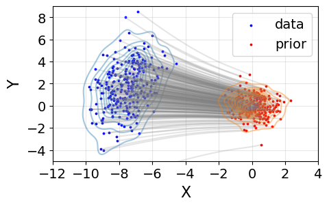
(a) GSB

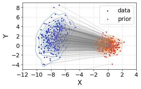
(b) VSDM

Figure 1: Gaussian SB (GSB) v.s. VSDM on the flow trajectories.

7.2 Synthetic Data

We test our variational Schrödinger diffusion models (VSDMs) on two synthetic datasets: spiral and checkerboard (detailed in section D.2.1). We include SGMs as the baseline models and aim to show the strength of VSDMs on general shapes with straighter trajectories. As such, we stretch the Y-axis of the spiral data by 8 times and the X-axis of the checkerboard data by 6 times and denote them by spiral-8Y and checkerboard-6X, respectively.

We adopt a monotone increasing $\{\beta_{nh}\}_{n=0}^{N-1}$ similar to Song et al. (2021b) and denote by $\beta_{\min}$ and $\beta_{\max}$ the minimum and maximum of $\{\beta_{nh}\}_{n=0}^{N-1}$. We fix $\zeta=0.75$ and $\beta_{\min}=0.1$ and we focus on the study with different $\beta_{\max}$. We find that SGMs work pretty well with $\beta_{\max}=10$ (SGM-10) on standard isotropic shapes. However, when it comes to spiral-8Y, the SGM-10 struggles to recover the boundary regions on the spiral-8Y data as shown in Figure 2 (top).

Generations of Anisotropic Shapes

To illustrate the effectiveness of our approach, Figure 2 (bottom) shows that VSDM-10 accurately reconstructs the edges of the spiral and generates high-quality samples.

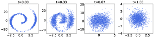
Figure 2: Variational Schrödinger diffusion models (VSDMs, bottom) v.s. SGMs (top) with the same hyperparameters ($\beta_{\max}=10$).

Straighter Trajectories

The SGM-10 fails to fully generate the anisotropic spiral-8Y and increasing $\beta_{\max}$ to 20 or 30 (SGM-20 and SGM-30) significantly alleviates this issue. However, we observe that excessive $\beta_{\max}$ values in SGMs compromise the straightness and leads to inefficient transport, especially in the X-axis of spiral-8Y.

(a) SGM-10

(b) SGM-20

(c) SGM-30

(d) VSDM-10

Figure 3: Probability flow ODE via VSDMs and SGMs. SGM with $\beta_{\max}=10$ is denoted by SGM-10 for convenience.

Instead of setting excessive $\beta_{\max}$ on both axes, our VSDM-10, by contrast, proposes conservative diffusion scales on the X-axis of spiral-8Y and explores more on the Y-axis of spiral-8Y. As such, we obtain around 40% improvement on the straightness in Figure 3 and Table 4.

Additional insights into a similar analysis of the checkboard dataset, convergence analysis, computational time, assessments of straightness, and evaluations via a smaller number of function evaluations (NFEs) can be found in Appendix D.2.

7.3 Image Data Modeling

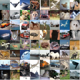
Figure 4: Unconditional generated samples from VSDM on CIFAR10 (32$\times 32$ resolution) trained from scratch.

Table 1: Convergence speed of FID values for VSDM.

K Images	0	10k	20k	30k	40k	50k	100k	150k	200k	converge
FID$\downarrow$ (NFE=35)	406.13	13.13	8.65	6.83	5.66	5.21	3.62	3.29	3.01	2.28

Experiment Setup

In this experiment, we evaluate the performance of VSDM on image modeling tasks. We choose the CIFAR10 datasetas representative image data to demonstrate the scalability of the proposed VSDM on generative modeling of high-dimensional distributions. We refer to the code base of FB-SDE (Chen et al., 2022b) and use the same forward diffusion process of the EDM model (Karras et al., 2022). Since the training of VSDM is an alternative manner between forward and backward training, we build our implementations based on the open-source diffusion distillation code base (Luo et al., 2024a) , which provides a high-quality empirical implementation of alternative training with EDM model on CIFAR10 data. To make the VSDM algorithm stable, we simplify the matrix ${\bf D}_{t}$ to be diagonal with learnable diagonal elements, which is the case as we introduced in Corollary 1. We train the VSDM model from scratch on two NVIDIA A100-80G GPUs for two days and generate images from the trained VSDM with the Euler–Maruyama numerical solver with 200 discretized steps for generation.

Table 2: CIFAR10 evaluation using sample quality (FID score). Our VSDM outperforms other optimal transport baselines by a large margin.

Class	Method	FID $\downarrow$
OT	VSDM (ours)	2.28
	SB-FBSDE (Chen et al., 2022b)	3.01
	DOT (Tanaka, 2019)	15.78
	DGflow (Ansari et al., 2020)	9.63
SGMs	SDE (Song et al. (2021b))	2.92
	ScoreFlow (Song et al., 2021a)	5.7
	VDM (Kingma et al., 2021)	4.00
	LSGM(Vahdat et al., 2021)	2.10
	EDM(Karras et al., 2022)	1.97

Performances.

We measure the generative performances in terms of the Fretchat Inception Score (FID (Heusel et al., 2017), the lower the better), which is a widely used metric for evaluating generative modeling performances.

Tables 2 summarize the FID values of VSDM along with other optimal-transport-based and score-based generative models on the CIFAR10 datasets (unconditional without labels). The VSDM outperforms other optimal transport-based models with an FID of 2.28. This demonstrates that the VSDM has applicable scalability to model high-dimensional distributions. Figure 4 shows some non-cherry-picked unconditional generated samples from VSDM trained on the CIFAR10 dataset.

Convergence Speed.

To demonstrate the convergence speed of VSDM along training processes, we record the FID values in Table 1 for a training trail with no warmup on CIFAR10 datasets (unconditional). We use a batch size of 256 and a learning rate of $1e-4$. We use the 2nd-order Heun numerical solver to sample. The result shows that VSDM has a smooth convergence performance.

7.4 Time Series Forecasting

We use multivariate probabilistic forecasting as a real-world conditional modeling task. Let $\{(t_{1},{\bf x}_{1}),\dots,(t_{n},{\bf x}_{n})\}$, ${\bf x}\in\mathbb{R}^{d}$, denote a single multivariate time series. Given a dataset of such time series we want to predict the next $P$ values ${\bf x}_{n+1},\dots,{\bf x}_{n+P}$. In probabilistic modeling, we want to generate forecasts from learned $p({\bf x}_{n+1:n+P}|{\bf x}_{1:n})$.

The usual approach is to have an encoder that represents a sequence ${\bf x}_{1:i}$ with a fixed-sized vector $\bm{h}_{i}\in\mathbb{R}^{h}$, $\forall i$, and then parameterize the output distribution $p({\bf x}_{i+1}|\bm{h}_{i})$. At inference time we encode the history into $\bm{h}_{n}$ and sample the next value from $p({\bf x}_{n+1}|\bm{h}_{n})$, then use ${\bf x}_{n+1}$ to get the updated $\bm{h}_{n+1}$ and repeat until we obtain ${\bf x}_{n+P}$.

In the previous works, the output distribution has been specified with a Copulas (Salinas et al., 2019) and denoising diffusion (Rasul et al., 2021). We augment our approach to allow conditional generation which requires only changing the model to include the conditioning vector $\bm{h}_{i}$. For that we adopt the U-Net architecture. We use the LSTM neural network as a sequence encoder.

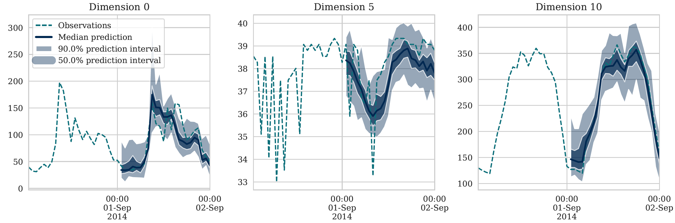
Figure 12: Example forecasts for Electricity (top), Exchange (middle), and Solar (bottom) datasets using our VSDM model. We show 3 out of 370, 8, and 137 dimensions, respectively.

We use three real-world datasets, as described in Appendix D.3. We compare to the SGM and the denoising diffusion approach from Rasul et al. (2021) which we refer to as DDPM. Table 3 shows that our method matches or outperforms the competitors. Figure 5 is a demo for conditional time series generation and more details are presented in Figure 12 to demonstrate the quality of the forecasts.

Table 3: Forecasting results (lower is better).

CRPS-sum	Electricity	Exchange rate	Solar
DDPM	0.026$\pm$0.007	0.012$\pm$0.001	0.506$\pm$0.058
SGM	0.045$\pm$0.005	0.012$\pm$0.002	0.413$\pm$0.045
VSDM (our)	0.038$\pm$0.006	0.008$\pm$0.002	0.395$\pm$0.011

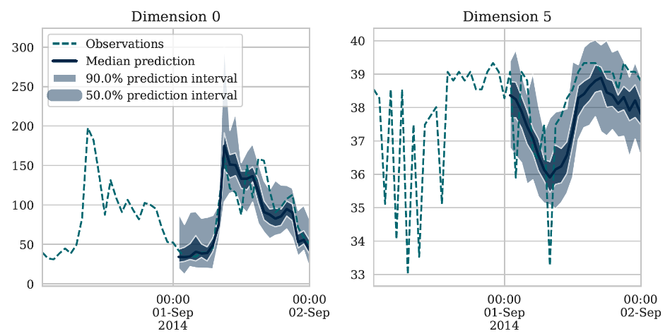
Figure 5: Example for Electricity for 2 (out of 370) dimensions.

8 Conclusions and Future Works

The Schrödinger bridge diffusion model offers a principled approach to solving optimal transport, but estimating the intractable forward score relies on implicit training through costly simulated trajectories. To address this scalability issue, we present the variational Schrödinger diffusion model (VSDM), utilizing linear variational forward scores for simulation-free training of backward score functions. Theoretical foundations leverage stochastic approximation theory, demonstrating the convergence of variational scores to local equilibrium and highlighting the variational gap in optimal transport. Empirically, VSDM showcases the strength of generating data with anisotropic shapes and yielding the desired straighter transport paths for reducing the number of functional evaluations. VSDM also exhibits scalability in handling large-scale image datasets without requiring warm-up initializations. In future research, we aim to explore the critically damped (momentum) acceleration (Dockhorn et al., 2022) and Hessian approximations to develop the “ADAM” alternative of diffusion models.

Impact Statement

This paper proposed a principled approach to accelerate the training and sampling of generative models using optimal transport. This work will contribute to developing text-to-image generation, artwork creation, and product design. However, it may also raise challenges in the fake-content generation and pose a threat to online privacy and security.

Supplementary Material for “Variational Schrödinger Diffusion Models”

In section A, we study the closed-form expression of matrix exponential for diagonal and time-invariant ${\bf D}_{t}$; In section B, we study the convergence of the adaptive diffusion process; In section C, we study the variational gap of the optimal transport and discuss its connections to Gaussian Schrödinger bridge; In section D, we present more details on the empirical experiments.

Notations:

$\mathcal{X}$ is the state space for the data ${\bf x}$; $\overleftarrow{{\bf x}}^{(k)}_{nh}$ is the $n$-th backward sampling step with a learning rate $h$ at the $k$-th stage. $\eta_{k}$ is the step size to optimize ${\mathrm{\mathbf{A}}}$. $\mathcal{A}$ is the (latent) state space of ${\mathrm{\mathbf{A}}}$; ${\mathrm{\mathbf{A}}}_{t}^{(k)}$ is the forward linear score estimator at stage $k$ and time $t$, ${\mathrm{\mathbf{A}}}_{t}^{\star}$ is the equilibrium of Eq.(25) at time $t$. $\nabla\overrightarrow{\mathcal{L}}_{t}$ is the random field in the stochastic approximation process and also the loss (10) at time $t$; $\nabla\overrightarrow{{\mathrm{\mathbf{L}}}}_{t}$ is the mean field with the equilibrium ${\mathrm{\mathbf{A}}}_{t}^{\star}$. Given a fixed ${\mathrm{\mathbf{A}}}_{t}^{(k)}$ at step $k$, $\nabla\log\overrightarrow{\rho}_{t}^{(k)}$ (resp. $\nabla\log\overrightarrow{\rho}_{t|0}^{(k)}$) is the (resp. conditional) forward score function of Eq.(11) at time $t$ and step $k$; ${\mathrm{\mathbf{A}}}_{t}^{(k)}$ yields the approximated score function $s_{t}^{(k)}$ and $\overleftarrow{\rho}_{t}^{(k)}$ is the distribution of the continuous-time interpolation of the discretized backward SDE (22).

Appendix A Closed-form Expression with Diagonal and Time-Invariant ${\bf D}_{t}$

In this section, we give the proof of Corollary 1.

Proof  Denote ${\bf D}_{t}=\bm{\Lambda}\coloneqq\operatorname{diag}(\bm{\lambda})$, where $\lambda_{i}\geq 0,~{}\forall 1\leq i\leq d$, and $\sigma_{t}^{2}\coloneqq\int_{0}^{t}\beta_{s}\mathrm{d}s$, then by Eq. (14), we have

$$\begin{pmatrix}{\mathrm{\mathbf{C}}}_{t}\\ {\mathrm{\mathbf{H}}}_{t}\end{pmatrix} =\exp\Bigg{[}\begin{pmatrix}-\frac{1}{2}[\beta{\bf D}]_{t}&[\beta{\mathrm{\mathbf{I}}}]_{t}\\ \bm{0}&\frac{1}{2}[\beta{\bf D}^{\intercal}]_{t}\end{pmatrix}\Bigg{]}\begin{pmatrix}{{\boldsymbol{\Sigma}}}_{0}\\ {{\mathrm{\mathbf{I}}}}\end{pmatrix}=\exp({\mathrm{\mathbf{M}}}_{t})\begin{pmatrix}{{\boldsymbol{\Sigma}}}_{0}\\ {{\mathrm{\mathbf{I}}}}\end{pmatrix}.$$

Here $[\beta{\bf D}]_{t}=\int_{0}^{t}\beta_{s}{\bf D}_{t}\mathrm{d}s=\sigma_{t}^{2}\bm{\Lambda}$. The matrix ${\mathrm{\mathbf{M}}}_{t}$ is defined as

$${\mathrm{\mathbf{M}}}_{t}=\begin{pmatrix}-\frac{1}{2}\sigma_{t}^{2}\bm{\Lambda}&\sigma_{t}^{2}\mathbf{I}\\ \bm{0}&\frac{1}{2}\sigma_{t}^{2}\bm{\Lambda}\end{pmatrix}$$

Therefore, we have

$${\mathrm{\mathbf{M}}}_{t}^{2}=\begin{pmatrix}(-\frac{1}{2}\sigma_{t}^{2}\bm{\Lambda})^{2}&\bm{0}\\ \bm{0}&(\frac{1}{2}\sigma_{t}^{2}\bm{\Lambda})^{2}\end{pmatrix},~{}~{}{\mathrm{\mathbf{M}}}_{t}^{3}=\begin{pmatrix}(-\frac{1}{2}\sigma_{t}^{2}\bm{\Lambda})^{3}&\sigma_{t}^{2}(\frac{1}{2}\sigma_{t}^{2}\bm{\Lambda})^{2}\\ \bm{0}&(\frac{1}{2}\sigma_{t}^{2}\bm{\Lambda})^{3}\end{pmatrix},~{}~{}$$

$${\mathrm{\mathbf{M}}}_{t}^{4}=\begin{pmatrix}(-\frac{1}{2}\sigma_{t}^{2}\bm{\Lambda})^{4}&\bm{0}\\ \bm{0}&(\frac{1}{2}\sigma_{t}^{2}\bm{\Lambda})^{4},~{}~{}\end{pmatrix},~{}~{}{\mathrm{\mathbf{M}}}_{t}^{5}=\begin{pmatrix}(-\frac{1}{2}\sigma_{t}^{2}\bm{\Lambda})^{5}&\sigma_{t}^{2}(\frac{1}{2}\sigma_{t}^{2}\bm{\Lambda})^{4}\\ \bm{0}&(\frac{1}{2}\sigma_{t}^{2}\bm{\Lambda})^{5}\end{pmatrix},~{}~{}...$$

According to the definition of matrix exponential, we have

$$\exp({\mathrm{\mathbf{M}}}_{t}) =[\mathbf{I}+\frac{1}{1!}{\mathrm{\mathbf{M}}}_{t}+\frac{1}{2!}{\mathrm{\mathbf{M}}}_{t}^{2}+\frac{1}{3!}{\mathrm{\mathbf{M}}}_{t}^{3}+...]$$

$$=\begin{pmatrix}\exp(-\frac{1}{2}\sigma_{t}^{2}\bm{\Lambda})&\Big{[}\sigma_{t}^{2}\mathbf{I}+\frac{1}{3!}\sigma_{t}^{2}(\frac{1}{2}\sigma_{t}^{2}\bm{\Lambda})^{2}+\frac{1}{5!}(\frac{1}{2}\sigma_{t}^{2}\bm{\Lambda})^{4}+...\Big{]}\\ \bm{0}&\exp(\frac{1}{2}\sigma_{t}^{2}\bm{\Lambda})\end{pmatrix}$$

$$=\begin{pmatrix}\exp(-\frac{1}{2}\sigma_{t}^{2}\bm{\Lambda})&\frac{\sigma_{t}^{2}}{\frac{1}{2}\sigma_{t}^{2}\bm{\Lambda}}\Big{[}(\frac{1}{2}\sigma_{t}^{2}\bm{\Lambda})^{1}+\frac{1}{3!}\sigma_{t}^{2}(\frac{1}{2}\sigma_{t}^{2}\bm{\Lambda})^{3}+\frac{1}{5!}(\frac{1}{2}\sigma_{t}^{2}\bm{\Lambda})^{5}+...\Big{]}\\ \bm{0}&\exp(\frac{1}{2}\sigma_{t}^{2}\bm{\Lambda})\end{pmatrix}$$

$$=\begin{pmatrix}\exp(-\frac{1}{2}\sigma_{t}^{2}\bm{\Lambda})&\bm{\Lambda}^{-1}\Big{[}\exp(\frac{1}{2}\sigma_{t}^{2}\bm{\Lambda})-\exp(-\frac{1}{2}\sigma_{t}^{2}\bm{\Lambda})\Big{]}\\ \bm{0}&\exp(\frac{1}{2}\sigma_{t}^{2}\bm{\Lambda})\end{pmatrix}.$$

Notice that, when we have ${{\boldsymbol{\Sigma}}}_{0}=\bm{0}$, the expression can be simplified as follows

$$\begin{pmatrix}{\mathrm{\mathbf{C}}}_{t}\\ {\mathrm{\mathbf{H}}}_{t}\end{pmatrix} =\exp({\mathrm{\mathbf{M}}}_{t})\begin{pmatrix}\bm{0}\\ {{\mathrm{\mathbf{I}}}}\end{pmatrix}=\begin{pmatrix}\bm{\Lambda}^{-1}\Big{[}\exp(\frac{1}{2}\sigma_{t}^{2}\bm{\Lambda})-\exp(-\frac{1}{2}\sigma_{t}^{2}\bm{\Lambda})\Big{]}\\ \exp(\frac{1}{2}\sigma_{t}^{2}\bm{\Lambda})\end{pmatrix}.$$

Therefore, ${\mathrm{\mathbf{C}}}_{t}{\mathrm{\mathbf{H}}}_{t}^{-1}=\bm{\Lambda}^{-1}\big{\{}\mathbf{I}-\exp(-\sigma_{t}^{2}\bm{\Lambda})\big{\}}$. As a result, the corresponding forward transition writes

$$\bm{\mu}_{t|0} =\exp(-\frac{1}{2}\sigma_{t}^{2}\bm{\Lambda}){\bf x}_{0}$$

$${\mathrm{\mathbf{L}}}_{t} =\sigma_{t}\bm{\Lambda}^{-\frac{1}{2}}\sqrt{\mathbf{I}-\exp(-\sigma_{t}^{2}\bm{\Lambda})}.$$

Appendix B Stochastic Approximation

Stochastic approximation (SA), also known as the Robbins–Monro algorithm (Robbins & Monro, 1951; Benveniste et al., 1990) offers a conventional framework for the study of adaptive algorithms. The stochastic approximation algorithm works by repeating the sampling-optimization iterations in the dynamic setting in terms of simulated trajectories. We present our algorithm in Algorithm 2.

Algorithm 2 The (dynamic) stochastic approximation (SA) algorithm. The (dynamic) SA is a theoretical formulation of Algorithm 1. We assume optimizing the loss function (16) yields proper score estimations $s^{(k+1)}_{t}$ at each stage $k$ and time $t$ to approximate $\nabla\log\overrightarrow{\rho}_{t}^{(k)}(\overrightarrow{{\bf x}}_{t}|\overrightarrow{{\bf x}}_{0})$ in Eq.(9b).

  repeat

     Simulation: Sample the backward process from (17) given a fixed ${\mathrm{\mathbf{A}}}_{nh}^{(k)}$

$$\overleftarrow{{\bf x}}^{(k+1)}_{(n-1)h}=\left(-\frac{1}{2}\big{(}{\mathrm{\mathbf{I}}}-2{\mathrm{\mathbf{A}}}_{nh}^{(k)}\big{)}\beta_{nh}\overleftarrow{{\bf x}}^{(k+1)}_{nh}-{\beta_{nh}}s^{(k+1)}_{nh}\big{(}\overleftarrow{{\bf x}}^{(k+1)}_{nh}\big{)}\right)h+\sqrt{\beta_{nh}h}{\boldsymbol{\xi}}_{n},$$ (22)

where $\overleftarrow{{\bf x}}^{(k+1)}_{(N-1)}\sim\mathrm{N}(\bm{0},{\boldsymbol{\Sigma}}^{(k)}_{(N-1)h|0})$, $n\in[1,2,\cdots,N-1]$ and $h$ is the learning rate for the backward sampling (17) via the Euler–Maruyama (EM) discretization. ${\boldsymbol{\xi}}_{n}$ denotes the standard Gaussian vector at the sampling iteration $n$.

     Optimization: Minimize the implicit forward loss function (10)

$${\mathrm{\mathbf{A}}}_{nh}^{(k+1)}={\mathrm{\mathbf{A}}}_{nh}^{(k)}-\eta_{k+1}\nabla\overrightarrow{\mathcal{L}}_{nh}({\mathrm{\mathbf{A}}}_{nh}^{(k)};\overleftarrow{{\bf x}}^{(k+1)}_{nh}),$$ (23)

where $\nabla\overrightarrow{\mathcal{L}}_{nh}({\mathrm{\mathbf{A}}}_{nh}^{(k)};\overleftarrow{{\bf x}}^{(k+1)}_{nh})$ is the (dynamic) random field and $\eta_{k}$ is the step size. $n\in\{0,1,\cdots,N-1\}$.

  until Stage $k=k_{\max}$

To facilitate the analysis, we assume we only make a one-step sampling in Eq.(23). Note that it is not required in practice and multiple-step extensions can be employed to exploit the cached data more efficiently. The theoretical extension is straightforward and omitted in the proof. We also slightly abuse the notation for convenience and generalize ${\mathrm{\mathbf{A}}}_{nh}$ to ${\mathrm{\mathbf{A}}}_{t}$.

Theoretically, the primary objective is to show the iterates (19) follow the trajectories of the dynamical system asymptotically:

$$\mathrm{d}{\mathrm{\mathbf{A}}}_{t}=\nabla\overrightarrow{{\mathrm{\mathbf{L}}}}_{t}({\mathrm{\mathbf{A}}}_{t})\mathrm{d}s,$$ (24)

where $\nabla\overrightarrow{{\mathrm{\mathbf{L}}}}_{t}({\mathrm{\mathbf{A}}}_{t})$ is the mean field defined as follows:

$$\begin{split}\nabla\overrightarrow{{\mathrm{\mathbf{L}}}}_{t}({\mathrm{\mathbf{A}}}_{t})&=\int_{{\mathcal{X}}}\nabla\overrightarrow{\mathcal{L}}_{t}({\mathrm{\mathbf{A}}}_{t};\overleftarrow{{\bf x}}^{(\cdot)}_{t})\overleftarrow{\rho}_{t}(\mathrm{d}\overleftarrow{{\bf x}}^{(\cdot)}_{t}).\end{split}$$ (25)

We denote by ${\mathrm{\mathbf{A}}}_{t}^{\star}$ the solution of $\nabla\overrightarrow{{\mathrm{\mathbf{L}}}}_{t}({\mathrm{\mathbf{A}}}_{t}^{\star})=\bm{0}$. Since the samples simulated from $\overleftarrow{\rho}_{t}$ are slightly biased due to the convergence of forward process, discretization error, and score estimation errors as shown in Theorem 1. We expect the mean field is also biased with a perturbed equilibrium. However, by the perturbation theory (Vanden-Eijnden, 2001), the perturbation is mild and controlled by the errors in Theorem 1. Hence although ${\mathrm{\mathbf{A}}}_{t}^{\star}$ is not the optimal linear solution in terms of optimal transport, it still yields efficient transportation plans.

Since the exclusive (reverse) KL divergence is known to approximate a single mode (denoted by ${\mathrm{\mathbf{A}}}_{t}^{\star}$) in fitting multi-modal distributions, we proceed to assume the following regularity conditions for the solution ${\mathrm{\mathbf{A}}}_{t}^{\star}$ and the neighborhood of ${\mathrm{\mathbf{A}}}_{t}^{\star}$.

Assumption A1 (Regularity).

(Positive definiteness) For any $t\geq 0$ and ${\mathrm{\mathbf{A}}}_{t}\in\mathcal{A}$, there exists a constant $\lambda_{\min}>0$ s.t. $\lambda_{\min}{\mathrm{\mathbf{I}}}\preccurlyeq{\bf D}_{t}={\mathrm{\mathbf{I}}}-2{\mathrm{\mathbf{A}}}_{t}$, where ${\mathrm{\mathbf{A}}}\preccurlyeq{\mathrm{\mathbf{B}}}$ means ${\mathrm{\mathbf{B}}}-{\mathrm{\mathbf{A}}}$ is semi positive definite. (Locally strong convexity) For any stable local minimum ${\mathrm{\mathbf{A}}}_{t}^{\star}$ with $\nabla\overrightarrow{{\mathrm{\mathbf{L}}}}_{t}({\mathrm{\mathbf{A}}}_{t}^{\star})=\bm{0}$, there is always a neighborhood ${\mathrm{\mathbf{\Theta}}}$ s.t. ${\mathrm{\mathbf{A}}}_{t}^{\star}\in{\mathrm{\mathbf{\Theta}}}\subset\mathcal{A}$ and $\overrightarrow{{\mathrm{\mathbf{L}}}}_{t}$ is strongly convex in ${\mathrm{\mathbf{\Theta}}}$, i.e. there exists fixed constants $M>m>0$ s.t. for $\forall{\mathrm{\mathbf{A}}}\in{\mathrm{\mathbf{\Theta}}}$, $m{\mathrm{\mathbf{I}}}\preccurlyeq\frac{\partial^{2}\overrightarrow{{\mathrm{\mathbf{L}}}}_{t}}{\partial{\mathrm{\mathbf{A}}}^{2}}({\mathrm{\mathbf{A}}})\preccurlyeq M{\mathrm{\mathbf{I}}}$.

The first part of the above assumption is standard and can be achieved by an appropriate regularization during the training; the second part only assumes the strong convexity for a small neighborhood ${\mathrm{\mathbf{\Theta}}}$ of the optimum ${\mathrm{\mathbf{A}}}_{t}^{\star}$. As such, when conditions for Eq.(31) hold, we can apply the induction method to make sure all the subsequent iterates of ${\mathrm{\mathbf{A}}}_{t}^{(k)}$ stay in the same region ${\mathrm{\mathbf{\Theta}}}$ and converge to the local minimum ${\mathrm{\mathbf{A}}}_{t}^{\star}$. For future works, we aim to explore the connection between $m$ and $\lambda_{\min}$.

Next, we lay out three standard assumptions following Chen et al. (2023a) to conduct our analysis. Similar results are studied by Lee et al. (2022); Chen et al. (2022a) with different score assumptions.

Assumption A2 (Lipschitz Score).

The score function $\nabla\log\overrightarrow{\rho}_{t}$ ($\nabla\log\overrightarrow{\rho}_{t,{\mathrm{\mathbf{A}}}}$) is $L$-Lipschitz in both ${\bf x}$ and ${\mathrm{\mathbf{A}}}$ for any $t\in[0,T]$. For any ${\mathrm{\mathbf{A}}},{\mathrm{\mathbf{B}}}\in\mathcal{A}$ and any ${\bf x},{\bf y}\in\mathcal{X}$, we have

$$\begin{split}\|\nabla\log\overrightarrow{\rho}_{t,{\mathrm{\mathbf{A}}}}({\bf x})-\nabla\log\overrightarrow{\rho}_{t,{\mathrm{\mathbf{A}}}}({\bf y})\|_{2}&\leq L\|{\bf x}-{\bf y}\|_{2}\\ \|\nabla\log\overrightarrow{\rho}_{t,{\mathrm{\mathbf{A}}}}({\bf x})-\nabla\log\overrightarrow{\rho}_{t,{\mathrm{\mathbf{B}}}}({\bf y})\|_{2}&\leq L\|{\mathrm{\mathbf{A}}}-{\mathrm{\mathbf{B}}}\|\\ \end{split}$$

where $\|\cdot\|_{2}$ is the standard $L^{2}$ norm and $\|\cdot\|$ is matrix norm.

Assumption A3 (Second Moment Bound).

The data distribution has a bounded second moment $\mathfrak{m}_{2}^{2}:=\mathbb{E}_{\rho_{\text{data}}}[\|\cdot\|_{2}^{2}]<\infty$.

Assumption A4 (Score Estimation Error).

For all $t\in[0,T]$, and any ${\mathrm{\mathbf{A}}}_{t}$, we have some estimation error .

$$\mathbb{E}_{\overrightarrow{\rho}_{t}}[\|s_{t}-\nabla\log\overrightarrow{\rho}_{t}\|_{2}^{2}]\leq\epsilon_{\text{score}}^{2}.$$

We first use the multivariate diffusion to train our score estimators $\{s^{(k)}_{t}\}_{n=0}^{N-1}$ via the loss function (16) based on the pre-specified ${\mathrm{\mathbf{A}}}_{t}^{(k)}$. Following Chen et al. (2023a), we can show the generated samples based on $\{s^{(k)}_{t}\}_{n=0}^{N-1}$ are close in distribution to the ideal samples in Theorem 1. The novelty lies in the extension of single-variate diffusions to multi-variate diffusions.

Next, we use the stochastic approximation theory to prove the convergence of ${\mathrm{\mathbf{A}}}_{t}^{(k)}$ to a local equilibrium ${\mathrm{\mathbf{A}}}_{t}^{\star}$ in Theorem 2. In the end, we adapt Theorem 1 again to show the adaptively generated samples are asymptotically close to the samples based on the optimal ${\mathrm{\mathbf{A}}}_{t}^{\star}$ in Theorem 3, which further optimizes the transportation plans through a variational formulation. To facilitate the understanding, we summarize the details as follows

$$\begin{split}&\small{\text{Sample via ${\mathrm{\mathbf{A}}}_{t}^{(k)}$}}\qquad\qquad\qquad\text{Random Field}\qquad\qquad\ \text{Mean Field}\qquad\qquad\quad\text{Convergence of ${\mathrm{\mathbf{A}}}_{t}^{(k)}$}\qquad\quad\quad\text{Sample via ${\mathrm{\mathbf{A}}}_{t}^{\star}$}\\ &\footnotesize{\text{$s_{t}^{(k)}$}\xRightarrow[\text{Theorem \ref{theorem:quality_of_data}}]{\text{Backward Sampling}}\nabla\overrightarrow{\mathcal{L}}_{t}({\mathrm{\mathbf{A}}}_{t}^{(k)};\overleftarrow{{\bf x}}^{(k+1)}_{t})\xRightarrow{\text{Eq.\eqref{mean_field_perturbed}}}\nabla\overrightarrow{{\mathrm{\mathbf{L}}}}_{t}({\mathrm{\mathbf{A}}}_{t}^{(k)})\xRightarrow[\text{Theorem \ref{theorem_L2_convergence}}]{\text{Convergence }}{\mathrm{\mathbf{A}}}_{t}^{(k)}\rightarrow{\mathrm{\mathbf{A}}}_{t}^{\star}\xRightarrow[\text{Theorem \ref{theorem_adaptive_sampling}}]{\text{Adaptive Sampling}}\text{$\lim_{k\rightarrow\infty}\overleftarrow{{\bf x}}_{t}^{(k+1)}$}}.\end{split}$$

Proof of Sketch

• Part B.1: The generated samples (backward trajectories) approximate the ideal samples from the fixed ${\mathrm{\mathbf{A}}}_{t}^{(k)}$.

• Part B.2: We employ the SA theory to show the convergence ${\mathrm{\mathbf{A}}}_{t}^{(k)}$ to the optimal estimator ${\mathrm{\mathbf{A}}}_{t}^{\star}$.

• Part B.3: The adaptively generated samples approximate the ideal samples from the optimal ${\mathrm{\mathbf{A}}}_{t}^{\star}$ asymptotically.

B.1 Convergence of Approximated Samples with a Fixed ${\mathrm{\mathbf{A}}}_{t}$

The following result is majorly adapted from Theorem 2.1 of Chen et al. (2023a), where the single-variate diffusions are extended to the general multi-variate diffusions.

Recall that the forward samples ${\bf x}_{t}$ are sampled by (11) given a fixed ${\mathrm{\mathbf{A}}}_{t}$, we denote the density of ${\bf x}_{t}$ by $\overrightarrow{\rho}_{t}$ with $\overrightarrow{\rho}_{0}=\rho_{\text{data}}$. To facilitate the proof, we introduce an auxiliary variable ${\bf y}_{t}$ simulated from (11) with ${\bf y}_{0}\sim\mathrm{N}(\bm{0},{\mathrm{\mathbf{I}}})$ such that ${\bf y}_{t}$ is always a Gaussian distribution at time $t$ and $\mathrm{KL}(\rho_{\text{data}}\|\mathrm{N}(\bm{0},{\mathrm{\mathbf{I}}}))$ is well defined (not applicable to deterministic initializations for ${\bf y}_{0}$). We denote the auxiliary distribution of ${\bf y}_{t}$ at time $t$ by $\overrightarrow{\rho}_{t}^{\circ}$. For a fixed $T>0$ and score estimations $s_{t}$, let $\overleftarrow{\rho}_{t}$ be the distribution of the continuous-time interpolation of the discretized backward SDE from $t=T$ to $0$ with $\overleftarrow{\rho}_{T}=\overrightarrow{\rho}_{T}^{\circ}$. Then generation quality is measured by the distance between $\overleftarrow{\rho}_{0}$ and $\rho_{\text{data}}$.

Theorem 1 (Generation quality).

Assume assumptions A2, A3, and A4 hold. Given a fixed ${\mathrm{\mathbf{A}}}_{t}$ by assumption A1, the generated data distribution via the EM discretization of Eq.(17) is close to the data distributions $\rho_{\text{data}}$ such that

$$\mathrm{TV}(\overleftarrow{\rho}_{0},\rho_{\text{data}})\lesssim\underbrace{\sqrt{\mathrm{KL}(\rho_{\text{data}}\|\gamma^{d})}\exp(-T)}_{\text{convergence of forward process}}+\underbrace{(L\sqrt{dh}+\mathfrak{m}_{2}h)\sqrt{T}}_{\text{EM discretization}}+\underbrace{\epsilon_{\text{score}}\sqrt{T}}_{\text{score estimation}},$$

where $\gamma^{d}$ is the standard Gaussian distribution.

Proof  Following Chen et al. (2023a), we employ the chain rule for KL divergence and obtain:

$$\mathrm{KL}(\rho_{\text{data}}\|\overleftarrow{\rho}_{0})\leq\mathrm{KL}(\overrightarrow{\rho}_{T}\|\overleftarrow{\rho}_{T})+\mathbb{E}_{\overrightarrow{\rho}_{T}({\bf x})}[\mathrm{KL}(\overrightarrow{\rho}_{0|T}(\cdot\|{\bf x})|\overleftarrow{\rho}_{0|T}(\cdot\|{\bf x})],$$

where $\overrightarrow{\rho}_{0|T}$ is the conditional distribution of ${\bf x}_{0}$ given ${\bf x}_{T}$ and likewise for $\overleftarrow{\rho}_{0|T}$. Note that the two terms correspond to the convergence of the forward and reverse process respectively. We proceed to prove that

$$\text{Part I: Forward process}\quad\quad\mathrm{KL}(\overrightarrow{\rho}_{T}\|\overleftarrow{\rho}_{T})=\mathrm{KL}(\overrightarrow{\rho}_{T}\|\overrightarrow{\rho}_{T}^{\circ})\lesssim\mathrm{KL}(\rho_{\text{data}}\|\gamma^{d})e^{-T},$$

$$\text{Part II: Backward process}\quad\mathbb{E}_{\overrightarrow{\rho}_{T}({\bf x})}[\mathrm{KL}(\overrightarrow{\rho}_{0|T}(\cdot|{\bf x})\|\overleftarrow{\rho}_{0|T}(\cdot|{\bf x})]\lesssim(L^{2}dh+m_{2}^{2}h^{2})T+\epsilon_{\text{score}}^{2}T.$$

Part I: By the Fokker-Plank equation, we have

$$\frac{\mathrm{d}}{\mathrm{d}t}\mathrm{KL}(\overrightarrow{\rho}_{t}\|\overrightarrow{\rho}_{t}^{\circ}) =-\frac{1}{2}\beta_{t}J_{\overrightarrow{\rho}_{t}^{\circ}}(\overrightarrow{\rho}_{t})$$

where

$$J_{\overrightarrow{\rho}_{t}^{\circ}}(\overrightarrow{\rho}_{t})=\int\overrightarrow{\rho}_{t}(x)\bigg{\|}\nabla\ln\frac{\overrightarrow{\rho}_{t}({\bf x})}{\overrightarrow{\rho}_{t}^{\circ}({\bf x})}\bigg{\|}^{2}\mathrm{d}{\bf x}$$

is the relative Fisher information of $\overrightarrow{\rho}_{t}$ with respect to $\overrightarrow{\rho}_{t}^{\circ}$. Note that for all $t\geq 0$, $\overrightarrow{\rho}_{t}^{\circ}$ is a Gaussian distribution and hence satisfies the log-Sobolev inequality  (Vempala & Wibisono, 2022). It follows that

$$\mathrm{KL}(\overrightarrow{\rho}_{t}\|\overrightarrow{\rho}_{t}^{\circ})\leq\frac{1}{2\alpha_{t}}J_{\overrightarrow{\rho}_{t}^{\circ}}(\overrightarrow{\rho}_{t}),$$

where $\alpha_{t}$ is the log-Sobolev constant of $\overrightarrow{\rho}_{t}^{\circ}$. This implies that

$$\frac{\mathrm{d}}{\mathrm{d}t}\mathrm{KL}(\overrightarrow{\rho}_{t}\|\overrightarrow{\rho}_{t}^{\circ})\leq-\alpha_{t}\beta_{t}\mathrm{KL}(\overrightarrow{\rho}_{t}\|\overrightarrow{\rho}_{t}^{\circ}).$$

Applying the Grönwall’s inequality yields

$$\mathrm{KL}(\overrightarrow{\rho}_{t}\|\overrightarrow{\rho}_{t}^{\circ})\leq e^{-\int_{0}^{t}\alpha_{s}\beta_{s}\mathrm{d}s}\mathrm{KL}(\overrightarrow{\rho}_{0}\|\overrightarrow{\rho}_{0}^{\circ})\leq e^{-\alpha\int_{0}^{t}\beta_{s}\mathrm{d}s}\mathrm{KL}(\overrightarrow{\rho}_{0}\|\overrightarrow{\rho}_{0}^{\circ}),$$

where the last inequality is followed by Lemma 1 and $\alpha$ is a lower bound estimate of the LSI constant $\inf_{t\in[0,T]}\alpha_{t}$.

Then by Pinsker’s Inequality, we have

$$\text{TV}(\overrightarrow{\rho}_{t},\overrightarrow{\rho}_{t}^{\circ})\leq\sqrt{2\mathrm{KL}(\overrightarrow{\rho}_{t}\|\overrightarrow{\rho}_{t}^{\circ})}\leq\sqrt{2e^{-\alpha\int_{0}^{t}\beta_{s}\mathrm{d}s}\mathrm{KL}(\overrightarrow{\rho}_{0}\|\overrightarrow{\rho}_{0}^{\circ})}\lesssim\sqrt{\mathrm{KL}(\rho_{\text{data}}\|\gamma^{d})}\exp(-t).$$

Part II: The proof for the convergence of the reverse process is essentially identical to Theorem 2.1 of Chen et al. (2023a), with the only potential replacements being instances of $\|{\bf x}_{t}-{\bf x}_{kh}\|_{2}$ with $\|{\bf D}_{T-t}({\bf x}_{t}-{\bf x}_{kh})\|_{2}$. However, they are equivalent due to Assumption A1. Therefore, we omit the proof here.

In conclusion, the convergence follows that

$$\mathrm{KL}(\rho_{\text{data}}\|\overleftarrow{\rho}_{0})\lesssim\mathrm{KL}(\rho_{\text{data}}\|\gamma^{d})e^{-T}+(L^{2}dh+m_{2}^{2}h^{2})T+\epsilon_{\text{score}}T.$$

And we obtain the final result using the Pinsker’s Inequality. ∎

Lemma 1 (Lower bound of the log-Sobolev constant).

Under the same assumptions and setups in Theorem 1, we have

$$\inf_{t\in[0,T]}\alpha_{t}\geq\min\{1,\lambda_{\min}\}=:\alpha\sim O(1).$$

Proof  Consider the auxiliary process for ${\bf y}_{t}$:

• Randomness from the initial: By the mean diffusion in Eq.(12a), the conditional mean diffusion of ${\bf y}_{t}$ at time $t$, denoted by $\mu_{t,{\bf y}}$, follows that $\mu_{t,{\bf y}}=\mathbb{D}_{t}\mu_{0,{\bf y}}$, where $\mathbb{D}_{t}=e^{-\frac{1}{2}[\beta{\bf D}]_{t}}$. Since ${\bf y}_{0}\sim\mathrm{N}(\bm{0},{\mathrm{\mathbf{I}}})$, we know $\mu_{t,{\bf y}}\sim\mathrm{N}(\bm{0},\mathbb{D}_{t}\mathbb{D}_{t}^{\intercal})$.

• Randomness from Brownian motion: the covariance diffusion induced by Brownian motion follows from ${\boldsymbol{\Sigma}}_{t|0}$ in Eq.(12b).

Since ${\bf y}_{0}\sim\mathrm{N}(\bm{0},{\mathrm{\mathbf{I}}})$ and ${\bf y}_{t}$ is an OU process in Eq.(11), we know that ${\bf y}_{t}$ is always a Gaussian distribution at time $t\geq 0$ with mean $\bm{0}$. As such, we know that

$$\overrightarrow{\rho}_{t}^{\circ}=\mathrm{N}(\bm{0},\mathbb{D}_{t}\mathbb{D}_{t}^{\intercal}+{\boldsymbol{\Sigma}}_{t|0}).$$ (26)

It follows that

$$\text{TV}(\overrightarrow{\rho}_{t},\overrightarrow{\rho}_{t}^{\circ})\leq\sqrt{2e^{-\int_{0}^{t}\alpha_{s}\beta_{s}\mathrm{d}s}\mathrm{KL}(\overrightarrow{\rho}_{0}\|\overrightarrow{\rho}_{0}^{\circ})}.$$

Now we need to bound the log-Sobolev constant $\alpha_{t}$ of $\overrightarrow{\rho}_{t}^{\circ}$. Let ${\boldsymbol{\Sigma}}_{t}=\mathbb{D}_{t}\mathbb{D}_{t}^{\intercal}+{\boldsymbol{\Sigma}}_{t|0}$. Recall that if a distribution $p$ is $\alpha$-strongly log-concave, then it satisfies the log-Sobolev inequality (LSI) with LSI constant $\alpha$ (Vempala & Wibisono, 2022). So for the Gaussian distribution $\overrightarrow{\rho}_{t}^{\circ}$, it suffices to bound the (inverse of) smallest eigenvalue of ${\boldsymbol{\Sigma}}_{t}$. Recall from Eq.(12b) that ${\boldsymbol{\Sigma}}_{t}$ satisfies the ODE

$$\frac{\mathrm{d}{\boldsymbol{\Sigma}}_{t}}{\mathrm{d}t}=-\frac{1}{2}\beta_{t}({\bf D}_{t}{\boldsymbol{\Sigma}}_{t}+{\boldsymbol{\Sigma}}_{t}{\bf D}_{t}^{\intercal})+\beta_{t}{\mathrm{\mathbf{I}}},\quad{\boldsymbol{\Sigma}}_{0}={\mathrm{\mathbf{I}}}.$$

Fix a normalized vector ${\bf x}\in\mathbb{R}^{d}$ and denote $u_{t}={\bf x}^{\intercal}{\boldsymbol{\Sigma}}_{t}{\bf x}$ for $t\in[0,T]$. By the cyclical property of the trace, we have

$${\bf x}^{\intercal}{\bf D}_{t}{\boldsymbol{\Sigma}}_{t}{\bf x}=\text{Tr}({\bf x}^{\intercal}{\bf D}_{t}{\boldsymbol{\Sigma}}_{t}{\bf x})=\text{Tr}({\bf D}_{t}{\boldsymbol{\Sigma}}_{t}{\bf x}{\bf x}^{\intercal})\geq\lambda_{\min}\text{Tr}({\boldsymbol{\Sigma}}_{t}{\bf x}{\bf x}^{\intercal})=\lambda_{\min}u_{t}.$$

It follows that

$$\frac{\mathrm{d}u_{t}}{\mathrm{d}t}\leq-\lambda_{\min}\beta_{t}u_{t}+\beta_{t}.$$

Applying the Grönwall’s inequality tells us that

$$u_{t}\leq\frac{1}{\lambda_{\min}}(1-e^{-\lambda_{\min}\int_{0}^{T}\beta_{s}\mathrm{d}s})+e^{-\lambda_{\min}\int_{0}^{T}\beta_{s}\mathrm{d}s}\leq\max\{1,1/\lambda_{\min}\}.$$

Since ${\bf x}$ can be any normalized vector, we have that the largest eigenvalue of ${\boldsymbol{\Sigma}}_{t}$ is bounded by $\max\{1,1/\lambda_{\min}\}$ and hence

$$\inf_{t\in[0,T]}\alpha_{t}\geq\min\{1,\lambda_{\min}\}=:\alpha\sim O(1),$$

where $\alpha_{t}$ is the log-Sobolev constant of $\overrightarrow{\rho}_{t}^{\circ}$. ∎

Remark:

In our theoretical analysis, we introduced an auxiliary variable ${\bf y}_{0}\sim\gamma^{d}$ to make sure $\mathrm{KL}(\rho_{\text{data}}\|\gamma^{d})$ is well defined. Moreover, the distribution of ${\bf y}_{T}$ is set to $\overrightarrow{\rho}_{T}^{\circ}$ in Eq.(26). However, we emphasize that the introduction of ${\bf y}_{t}$ is only for theoretical analysis and we adopt a simpler prior $\mathrm{N}(\bm{0},{\boldsymbol{\Sigma}}_{T|0})$ instead of $\mathrm{N}(\bm{0},\mathbb{D}_{T}\mathbb{D}_{T}^{\intercal}+{\boldsymbol{\Sigma}}_{T|0})$ in Eq.(26) for convenience.

B.2 Part II: Stochastic Approximation Convergence

${\mathrm{\mathbf{A}}}_{t}^{(k)}$ converges to ${\mathrm{\mathbf{A}}}_{t}^{\star}$ by tracking a mean-field ODE with some fluctuations along the trajectory. Before we prove the convergence, we need to show the stability property of the mean-field ODE such that small fluctuations of earlier iterates do not affect the convergence to the equilibrium. To that end, we construct a Lyapunov function $\mathbb{V}_{t}({\mathrm{\mathbf{A}}})=\frac{1}{2}m\|{\mathrm{\mathbf{A}}}-{\mathrm{\mathbf{A}}}_{t}^{\star}\|_{2}^{2}$ to analyze the local stability condition of the solution. This result shows that when the solution is close to the equilibrium ${\mathrm{\mathbf{A}}}_{t}^{\star}\in{\mathrm{\mathbf{\Theta}}}\subset{\mathrm{\mathbf{A}}}$, ${\mathrm{\mathbf{A}}}_{t}$ will asymptotically track the trajectory of the mean field (24) within ${\mathrm{\mathbf{\Theta}}}$ when the step size $\eta_{k}\rightarrow 0$.

Lemma 2 (Local stabiltity).

Assume the assumptions A1 and A2 hold. For any ${\mathrm{\mathbf{A}}}\in{\mathrm{\mathbf{\Theta}}}$, the solution satisfies a local stability condition such that

$$\langle{\mathrm{\mathbf{A}}}-{\mathrm{\mathbf{A}}}_{t}^{\star},\nabla\mathbb{V}_{t}({\mathrm{\mathbf{A}}})\rangle=\langle{\mathrm{\mathbf{A}}}-{\mathrm{\mathbf{A}}}^{\star},\nabla\overrightarrow{{\mathrm{\mathbf{L}}}}_{t}({\mathrm{\mathbf{A}}})\rangle\geq m\|{\mathrm{\mathbf{A}}}-{\mathrm{\mathbf{A}}}^{\star}\|_{2}^{2}.$$

Proof  By the smoothness assumption A2 and Taylor expansion, for any ${\mathrm{\mathbf{A}}}\in{\mathrm{\mathbf{\Theta}}}$, we have

$$\nabla\overrightarrow{{\mathrm{\mathbf{L}}}}_{t}({\mathrm{\mathbf{A}}})=\nabla\overrightarrow{{\mathrm{\mathbf{L}}}}_{t}({\mathrm{\mathbf{A}}}^{\star})+\textbf{Hess}\big{[}\overrightarrow{{\mathrm{\mathbf{L}}}}_{t}\big{(}\widetilde{\mathrm{\mathbf{A}}}\big{)}\big{]}({\mathrm{\mathbf{A}}}-{\mathrm{\mathbf{A}}}^{\star})=\textbf{Hess}\big{[}\overrightarrow{{\mathrm{\mathbf{L}}}}_{t}\big{(}\widetilde{\mathrm{\mathbf{A}}}\big{)}\big{]}({\mathrm{\mathbf{A}}}-{\mathrm{\mathbf{A}}}^{\star}),$$ (27)

where $\textbf{Hess}\big{[}\overrightarrow{{\mathrm{\mathbf{L}}}}_{t}\big{(}{\mathrm{\mathbf{A}}}\big{)}\big{]}$ denotes the Hessian of $\overrightarrow{{\mathrm{\mathbf{L}}}}_{t}$ with ${\mathrm{\mathbf{A}}}$ at time $t$; $\widetilde{\mathrm{\mathbf{A}}}$ is some value between ${\mathrm{\mathbf{A}}}$ and ${\mathrm{\mathbf{A}}}_{t}^{\star}$ by the mean-value theorem. Next, we can get

$$\langle{\mathrm{\mathbf{A}}}-{\mathrm{\mathbf{A}}}_{t}^{\star},\nabla\overrightarrow{{\mathrm{\mathbf{L}}}}_{t}({\mathrm{\mathbf{A}}})\rangle=\textbf{Hess}\big{[}\overrightarrow{{\mathrm{\mathbf{L}}}}_{t}\big{(}\widetilde{\mathrm{\mathbf{A}}}\big{)}\big{]}\|{\mathrm{\mathbf{A}}}-{\mathrm{\mathbf{A}}}^{\star}\|_{2}^{2}\geq m\|{\mathrm{\mathbf{A}}}-{\mathrm{\mathbf{A}}}^{\star}\|_{2}^{2},$$

where the last inequality follows by assumption A1. ∎

Additionally, we show the random field satisfies a linear growth condition to avoid blow up in tails.

Lemma 3 (Linear growth).

Assume the assumptions A2 and A3 hold. There exists a constant $C>0$ such that $\forall{\mathrm{\mathbf{A}}}_{t}^{(k)}\in{\mathrm{\mathbf{\Theta}}}$ at the SA step $k$ and time $t$, the random field is upper bounded in $L^{2}$ such that

$$\mathbb{E}[\|\nabla\overrightarrow{\mathcal{L}_{t}}({\mathrm{\mathbf{A}}}_{t}^{(k)},\overleftarrow{{\bf x}}^{(k+1)}_{t})\|^{2}_{2}|\mathcal{F}_{k}]\leq C(1+\|{\mathrm{\mathbf{A}}}^{(k)}_{t}-{\mathrm{\mathbf{A}}}^{\star}_{t}\|_{2}^{2}):=C(1+\|{\bf G}^{(k)}_{t}\|_{2}^{2}),$$

where the trajectory $\overleftarrow{{\bf x}}^{(k+1)}_{t}$ is simulated by (22); $\mathcal{F}_{k}$ is a $\sigma$-filtration formed by $(\overleftarrow{{\bf x}}_{t}^{(1)},{\mathrm{\mathbf{A}}}_{t}^{(1)},\overleftarrow{{\bf x}}_{t}^{(2)},{\mathrm{\mathbf{A}}}_{t}^{(2)},\cdots,\overleftarrow{{\bf x}}_{t}^{(k)},{\mathrm{\mathbf{A}}}_{t}^{(k)})$.

Proof  By the unbiasedness of the random field, we have

$$\mathbb{E}[\nabla\overrightarrow{\mathcal{L}}_{t}({\mathrm{\mathbf{A}}}_{t}^{(k)};\overleftarrow{{\bf x}}^{(k+1)}_{t})-\nabla\overrightarrow{{\mathrm{\mathbf{L}}}}_{t}({\mathrm{\mathbf{A}}}_{t}^{(k)})|\mathcal{F}_{k}]=\bm{0}.$$ (28)

It follows that

$$\begin{split}\mathbb{E}[\|\nabla\overrightarrow{\mathcal{L}}_{t}({\mathrm{\mathbf{A}}}_{t}^{(k)};\overleftarrow{{\bf x}}^{(k+1)}_{t})\|^{2}_{2}|\mathcal{F}_{k}]&=\mathbb{E}[\|\nabla\overrightarrow{\mathcal{L}}_{t}({\mathrm{\mathbf{A}}}_{t}^{(k)};\overleftarrow{{\bf x}}^{(k+1)}_{t})-\nabla\overrightarrow{{\mathrm{\mathbf{L}}}}_{t}({\mathrm{\mathbf{A}}}_{t}^{(k)})+\nabla\overrightarrow{{\mathrm{\mathbf{L}}}}_{t}({\mathrm{\mathbf{A}}}_{t}^{(k)}))\|^{2}_{2}|\mathcal{F}_{k}]\\ &=\mathbb{E}[\|\nabla\overrightarrow{\mathcal{L}}_{t}({\mathrm{\mathbf{A}}}_{t}^{(k)};\overleftarrow{{\bf x}}^{(k+1)}_{t})-\nabla\overrightarrow{{\mathrm{\mathbf{L}}}}_{t}({\mathrm{\mathbf{A}}}_{t}^{(k)})\|^{2}_{2}|\mathcal{F}_{k}]+\|\nabla\overrightarrow{{\mathrm{\mathbf{L}}}}_{t}({\mathrm{\mathbf{A}}}_{t}^{(k)})\|^{2}_{2}\\ &\leq\sup\mathbb{E}[\|\nabla\overrightarrow{\mathcal{L}}_{t}({\mathrm{\mathbf{A}}}_{t}^{(k)};\overleftarrow{{\bf x}}^{(k+1)}_{t})-\nabla\overrightarrow{{\mathrm{\mathbf{L}}}}_{t}({\mathrm{\mathbf{A}}}_{t}^{(k)})\|^{2}_{2}|\mathcal{F}_{k}]+M^{2}\|{\mathrm{\mathbf{A}}}_{t}^{(k)}-{\mathrm{\mathbf{A}}}_{t}^{\star}\|_{2}^{2},\end{split}$$ (29)

where the last inequality follows by assumption A1 and Eq.(27).

By assumption A2 and A3 and the process (17), we know $\sup\mathbb{E}[\|\nabla\overrightarrow{\mathcal{L}}_{t}({\mathrm{\mathbf{A}}}_{t}^{(k)};\overleftarrow{{\bf x}}^{(k+1)}_{t})-\nabla\overrightarrow{{\mathrm{\mathbf{L}}}}_{t}({\mathrm{\mathbf{A}}}_{t}^{(k)})\|^{2}_{2}|\mathcal{F}_{k}]<\infty$. Denote by $C:=\max\{\sup\mathbb{E}[\|\nabla\overrightarrow{\mathcal{L}}_{t}({\mathrm{\mathbf{A}}}_{t}^{(k)};\overleftarrow{{\bf x}}^{(k+1)}_{t})-\nabla\overrightarrow{{\mathrm{\mathbf{L}}}}_{t}({\mathrm{\mathbf{A}}}_{t}^{(k)})\|^{2}_{2}|\mathcal{F}_{k}],M^{2}\}$, we can conclude that

$$\mathbb{E}[\|\nabla\overrightarrow{\mathcal{L}}_{t}({\mathrm{\mathbf{A}}}_{t}^{(k)};\overleftarrow{{\bf x}}^{(k+1)}_{t})\|^{2}_{2}|\mathcal{F}_{k}]\leq C(1+\|{\mathrm{\mathbf{A}}}_{t}^{(k)}-{\mathrm{\mathbf{A}}}_{t}^{\star}\|_{2}^{2}).$$

∎

Next, we make standard assumptions on the step size following Benveniste et al. (1990) (page 245).

Assumption A5 (Step size).

The step size $\{\eta_{k}\}_{k\in\mathrm{N}}$ is a positive and decreasing sequence

$$\eta_{k}\rightarrow 0,\ \ \sum_{k=1}^{\infty}\eta_{k}=+\infty,\ \ \lim_{k\rightarrow\infty}\inf\left(2m\dfrac{\eta_{k}}{\eta_{k+1}}+\dfrac{\eta_{k+1}-\eta_{k}}{\eta^{2}_{k+1}}\right):=\kappa>0.$$

A standard choice is to set $\eta_{k}:=\frac{A}{k^{\alpha}+B}$ for some $\alpha\in(\frac{1}{2},1]$ and some suitable constants $A>0$ and $B>0$.

Theorem 2 (Convergence in $L^{2}$).

Assume assumptions A1, A2, A3, A4, and A5 hold. The variational score ${\mathrm{\mathbf{A}}}_{t}^{(k)}$ in algorithm 2 converges to a local minimizer ${\mathrm{\mathbf{A}}}_{t}^{\star}$. In other words, given a large enough $k\geq k_{0}$, where $\eta_{k_{0}}\leq\frac{1}{2}$, we have

$$\mathbb{E}[\|{\mathrm{\mathbf{A}}}_{t}^{(k)}-{\mathrm{\mathbf{A}}}_{t}^{\star}\|_{2}^{2}]\leq 2\eta_{k},$$

where the expectation is taken w.r.t samples from $\overleftarrow{\rho}_{t}^{(k)}$.

Proof  To show ${\mathrm{\mathbf{A}}}_{t}^{(k)}$ converges to ${\mathrm{\mathbf{A}}}_{t}^{\star}$, we first denote ${\bf G}_{t}^{(k)}={\mathrm{\mathbf{A}}}_{t}^{(k)}-{\mathrm{\mathbf{A}}}_{t}^{\star}$. Subtracting ${\mathrm{\mathbf{A}}}^{\star}$ on both sides of Eq.(23):

$${\bf G}_{t}^{(k+1)} ={\bf G}_{t}^{(k)}-\eta_{k+1}\nabla\overrightarrow{\mathcal{L}_{t}}({\mathrm{\mathbf{A}}}_{t}^{(k)};\overleftarrow{{\bf x}}^{(k+1)}_{t}).$$

By the unbiasedness of the random field, we have

$$\mathbb{E}[\nabla\overrightarrow{\mathcal{L}_{t}}({\mathrm{\mathbf{A}}}_{t}^{(k)};\overleftarrow{{\bf x}}_{t}^{(k+1)})-\nabla\overrightarrow{{\mathrm{\mathbf{L}}}}_{t}({\mathrm{\mathbf{A}}}_{t}^{(k)})|\mathcal{F}_{k}]=\bm{0}.$$ (30)

Taking the expectation in $L^{2}$, we have

$$\begin{split}\mathbb{E}[\|{\bf G}_{t}^{(k+1)}\|_{2}^{2}|\mathcal{F}_{k}]&=\|{\bf G}_{t}^{(k+1)}\|^{2}_{2}-2\eta_{k+1}\mathbb{E}\big{[}\langle{\bf G}_{t}^{(k)},\nabla\overrightarrow{\mathcal{L}_{t}}({\mathrm{\mathbf{A}}}^{(k)};\overleftarrow{{\bf x}}_{t}^{(k+1)})\rangle\big{]}+\eta_{k+1}^{2}\mathbb{E}\big{[}\|\nabla\overrightarrow{\mathcal{L}_{t}}({\mathrm{\mathbf{A}}}_{t}^{(k)};\overleftarrow{{\bf x}}^{(k+1)}_{t})\|^{2}_{2}|\mathcal{F}_{k}\big{]}\\ &=\|{\bf G}_{t}^{(k+1)}\|^{2}_{2}-2\eta_{k+1}\langle{\bf G}_{t}^{(k)},\nabla\overrightarrow{{\mathrm{\mathbf{L}}}}_{t}({\mathrm{\mathbf{A}}}_{t}^{(k)})\rangle+\eta_{k+1}^{2}\mathbb{E}\big{[}\|\nabla\overrightarrow{\mathcal{L}_{t}}({\mathrm{\mathbf{A}}}_{t}^{(k)};\overleftarrow{{\bf x}}^{(k+1)}_{t})\|^{2}_{2}|\mathcal{F}_{k}\big{]},\end{split}$$

where the second equality is followed by the unbiasedness property in Eq.(30).

Applying the stepsize assumption A5, we have

$$\eta_{k+1}-\eta_{k}+2m\eta_{k}\eta_{k+1}\geq C\eta_{k+1}^{2}.$$

Then for $\eta_{k}\leq\frac{1}{2}$, we have

$$2(\eta_{k+1}-\eta_{k}+\eta_{k}\eta_{k+1}(2m-\eta_{k+1}C))\geq C\eta_{k+1}^{2}.$$

Rewrite the above equation as follows

$$2\eta_{k+1}\geq(1-2\eta_{k+1}m+C\eta_{k+1}^{2})(2\eta_{k})+C\eta_{k+1}^{2}.$$

By the induction method, we have

• Given some large enough $k\geq k_{0}$, where $\eta_{k_{0}}\leq\frac{1}{2}$, ${\mathrm{\mathbf{A}}}_{t}^{(k)}$ is in some subset ${\mathrm{\mathbf{\Theta}}}$ of $\mathcal{A}$ that follows

  $$\mathbb{E}[\|{\bf G}_{t}^{k}\|_{2}^{2}]\leq 2\eta_{k}.$$ (31)

• Applying Eq.(B.2) and Eq.(B.2), respectively, we have

  $$\mathbb{E}[\|{\bf G}_{t}^{(k+1)}\|_{2}^{2}|\mathcal{F}_{k}] \leq(1-2\eta_{k+1}m)\mathbb{E}[\|{\bf G}_{t}^{(k)}\|_{2}^{2}]+\eta_{k+1}^{2}\mathbb{E}\big{[}\|\nabla\overrightarrow{\mathcal{L}_{t}}({\mathrm{\mathbf{A}}}_{t}^{(k)};\overleftarrow{{\bf x}}^{(k+1)}_{t})\|^{2}_{2}|\mathcal{F}_{k}\big{]}$$

  $$\leq(1-2\eta_{k+1}m+C\eta_{k+1}^{2})\mathbb{E}[\|{\bf G}_{t}^{(k)}\|_{2}^{2}]+C\eta_{k+1}^{2},$$

  $$\leq(1-2\eta_{k+1}m+C\eta_{k+1}^{2})(2\eta_{k})+C\eta_{k+1}^{2}$$ (32)

  $$\leq 2\eta_{k+1},$$

  where the first inequality is held by the stability property in Lemma 2 and the last inequality is followed by the growth property in Lemma 3.

Since ${\mathrm{\mathbf{A}}}_{t}^{\star},{\mathrm{\mathbf{A}}}_{t}^{(k)}\in{\mathrm{\mathbf{\Theta}}}$, Eq.(32) implies that ${\mathrm{\mathbf{A}}}_{t}^{(k+1)}\in{\mathrm{\mathbf{\Theta}}}$, which concludes the proof. ∎

B.3 Part III: Convergence of Adaptive Samples based on The Optimal ${\mathrm{\mathbf{A}}}^{\star}$

We have evaluated the sample quality in Theorem 1 based on a fixed ${\mathrm{\mathbf{A}}}_{t}$, which, however, may not be efficient in terms of transportation plans. To evaluate the sample quality in terms of the limiting optimal ${\mathrm{\mathbf{A}}}^{\star}$, we provide the result as follows:

Theorem 3.

Given assumptions A1-A5, the generated sample distribution at stage $k$ is $\epsilon$-close to the exact sample distribution $\overrightarrow{\rho}^{\star}_{T}$ based on the equilibrium ${\mathrm{\mathbf{A}}}_{t}^{\star}$ such that

$$\mathrm{TV}(\overleftarrow{\rho}^{\star}_{0},\rho_{\text{data}})\lesssim\sqrt{\mathrm{KL}(\rho_{\text{data}}\|\gamma^{d})}\exp(-T)+(L\sqrt{dh}+L\mathfrak{m}_{2}h)\sqrt{T}+(\epsilon_{\text{score}}+\sqrt{\eta_{k}})\sqrt{T}.$$

Proof  By assumption A4, for any ${\mathrm{\mathbf{A}}}^{(k)}_{t}\in\mathcal{A}$, we have

$$\mathbb{E}_{\overrightarrow{\rho}_{t}^{(k)}}[\|s_{t}^{(k)}-\nabla\log\overrightarrow{\rho}_{t}^{(k)}\|_{2}^{2}]\leq\epsilon_{\text{score}}^{2}.$$

Combining Theorem 2 and the smoothness assumption A2 of the score function $\nabla\log\overrightarrow{\rho}^{(k)}_{t}$ w.r.t ${\mathrm{\mathbf{A}}}^{(k)}_{t}$, we have

$$\mathbb{E}_{\overrightarrow{\rho}_{t}^{(k)}}[\|\nabla\log\overrightarrow{\rho}^{(k)}_{t}-\nabla\log\overrightarrow{\rho}^{\star}_{t}\|_{2}^{2}]\lesssim\eta_{k}.$$ (33)

It follows that the score function $s_{t}^{(k)}$ is also close to the optimal $\nabla\log\overrightarrow{\rho}_{t}^{\star}$ in the sense that

$$\begin{split}&\quad\ \mathbb{E}_{\overrightarrow{\rho}_{t}^{(k)}}[\|s_{t}^{(k)}-\nabla\log\overrightarrow{\rho}_{t}^{\star}\|_{2}^{2}]\\ &\lesssim\mathbb{E}_{\overrightarrow{\rho}_{t}^{(k)}}[\underbrace{\|s_{t}^{(k)}-\nabla\log\overrightarrow{\rho}_{t}\|_{2}^{2}}_{\text{by Assumption \ref{ass_score_estimation}}}]+\mathbb{E}_{\overrightarrow{\rho}^{(k)}_{t}}[\underbrace{\|\nabla\log\overrightarrow{\rho}_{t}^{(k)}-\nabla\log\overrightarrow{\rho}_{t}^{\star}\|_{2}^{2}}_{\text{by Eq.\eqref{closedness}}}]\\ &\lesssim\epsilon_{\text{score}}^{2}+\eta_{k}.\end{split}$$ (34)

Applying Theorem 1 with the adaptive score error in Eq.(LABEL:adaptive_score_error) to replace $\epsilon_{\text{score}}^{2}$ concludes the proof. ∎

Remark:

The convergence of samples based on the adaptive algorithms is slightly weaker than the standard one due to the adaptive update, but this is necessary because ${\mathrm{\mathbf{A}}}_{t}^{\star}$ is more transport efficient than a vanilla ${\mathrm{\mathbf{A}}}_{t}$.

Appendix C Variational Gap

Recall that the optimal forward SDE in the forward-backward SDEs (5) follows that

$${\mathrm{d}\overrightarrow{{\bf x}}_{t}}={\left[{\boldsymbol{f}}_{t}(\overrightarrow{{\bf x}}_{t})+\beta_{t}\nabla\log\overrightarrow{\psi}_{t}(\overrightarrow{{\bf x}}_{t})\right]\mathrm{d}t}+\sqrt{\beta_{t}}\mathrm{d}\overrightarrow{{\mathbf{w}}}_{t}.$$ (35)

The optimal variational forward SDE follows that

$$\mathrm{d}\overrightarrow{{\bf x}}_{t}=\left[{\boldsymbol{f}}_{t}(\overrightarrow{{\bf x}}_{t})+{\beta_{t}}{\mathrm{\mathbf{A}}}_{t}^{\star}\overrightarrow{{\bf x}}_{t}\right]\mathrm{d}t+\sqrt{\beta_{t}}\mathrm{d}\overrightarrow{{\mathbf{w}}}_{t}.$$ (36)

The variational forward SDE at the $k$-th step follows that

$$\mathrm{d}\overrightarrow{{\bf x}}_{t}=\left[{\boldsymbol{f}}_{t}(\overrightarrow{{\bf x}}_{t})+{\beta_{t}}{\mathrm{\mathbf{A}}}_{t}^{(k)}\overrightarrow{{\bf x}}_{t}\right]\mathrm{d}t+\sqrt{\beta_{t}}\mathrm{d}\overrightarrow{{\mathbf{w}}}_{t}.$$ (37)

Since we only employ a linear approximation of the forward score function, our transport is only sub-optimal. To assess the extent of this discrepancy, we leverage the Girsanov theorem to study the variational gap.

We denote the law of the processes by $\mathrm{L}(\cdot)$ in Eq.(35), ${\mathrm{L}}^{\star}(\cdot)$ in Eq.(36) and ${\mathrm{L}}^{(k)}(\cdot)$ in Eq.(37), respectively.

Theorem 4.

Assume assumptions A2 and A3 hold. Assume ${\boldsymbol{f}}_{t}$ and $\nabla\log\overrightarrow{\psi}_{t}$ are Lipschitz smooth and satisfy the linear growth condition. Assume the Novikov’s condition holds for $\forall{\mathrm{\mathbf{A}}}_{t}\in\mathcal{A}$, where $t\in[0,T]$:

$$\mathbb{E}\bigg{[}\exp\bigg{(}\frac{1}{2}\int_{0}^{T}\|{\beta_{t}}{\mathrm{\mathbf{A}}}_{t}\overrightarrow{{\bf x}}_{t}-\beta_{t}\nabla\log\overrightarrow{\psi}_{t}(\overrightarrow{{\bf x}}_{t})\|_{2}^{2}\mathrm{d}t\bigg{)}\bigg{]}<\infty.$$

The variational gap (VG) via the linear parametrization is upper bounded by

$$\begin{split}&{\mathrm{KL}({\mathrm{L}}\|{\mathrm{L}}^{\star})=\frac{1}{2}\int_{0}^{T}\mathbb{E}_{\overrightarrow{\rho}_{t}}\bigg{[}\beta_{t}\|{\mathrm{\mathbf{A}}}_{t}^{\star}\overrightarrow{{\bf x}}_{t}-\nabla\log\overrightarrow{\psi}_{t}(\overrightarrow{{\bf x}}_{t})\|_{2}^{2}\mathrm{d}t\bigg{]}}\\ &\mathrm{KL}({\mathrm{L}}\|{\mathrm{L}}^{(k)})\lesssim\eta_{k}+\mathrm{KL}({\mathrm{L}}\|{\mathrm{L}}^{\star}).\end{split}$$

Proof 

By Girsanov’s formula (Liptser & Shiryaev, 2001), the Radon–Nikodym derivative of ${\mathrm{L}}(\cdot)$ w.r.t. ${\mathrm{L}}^{\star}(\cdot)$ follows that

$$\frac{\mathrm{d}\mathrm{L}}{\mathrm{d}\mathrm{L}^{\star}}\big{(}\overrightarrow{{\bf x}}\big{)}=\exp\bigg{(}\int_{0}^{T}\sqrt{\beta_{t}}\bigg{(}{\mathrm{\mathbf{A}}}_{t}^{\star}\overrightarrow{{\bf x}}_{t}-\nabla\log\overrightarrow{\psi}_{t}(\overrightarrow{{\bf x}}_{t})\bigg{)}\mathrm{d}{\mathbf{w}}_{t}-\frac{1}{2}\int_{0}^{T}\beta_{t}\|{\mathrm{\mathbf{A}}}_{t}^{\star}\overrightarrow{{\bf x}}_{t}-\nabla\log\overrightarrow{\psi}_{t}(\overrightarrow{{\bf x}}_{t})\|_{2}^{2}\mathrm{d}t\bigg{)},$$

where ${\mathbf{w}}_{t}$ is the Brownian motion under the Wiener measure. Consider a change of measure (Øksendal, 2003; Chewi, 2023)

$${\mathbf{w}}_{t}=\widetilde{\mathbf{w}}_{t}-\mathrm{d}\big{[}{\mathbf{w}},{\mathrm{\mathbf{M}}}\big{]}_{t},\quad\mathrm{d}{\mathrm{\mathbf{M}}}_{t}=\big{\langle}\sqrt{\beta_{t}}\big{(}{\mathrm{\mathbf{A}}}_{t}^{\star}\overrightarrow{{\bf x}}_{t}-\nabla\log\overrightarrow{\psi}_{t}(\overrightarrow{{\bf x}}_{t})\big{)},\mathrm{d}{\mathbf{w}}_{t}\big{\rangle},$$

where $\widetilde{\mathbf{w}}_{t}$ is a $\mathrm{L}$-standard Brownian motion and satisfies martingale property under the $\mathrm{L}$ measure.

Now the variational gap is upper bounded by

$$\begin{split}\text{KL}({\mathrm{L}}(\cdot)\|\mathrm{L}^{\star}(\cdot))&=-\mathbb{E}_{\mathrm{L}(\cdot)}\bigg{[}\log\frac{\mathrm{d}\mathrm{L}(\cdot)}{\mathrm{d}\mathrm{L}^{\star}(\cdot)}\bigg{]}\\ &=\mathbb{E}_{\mathrm{L}(\cdot)}\bigg{[}\int_{0}^{T}\sqrt{\beta_{t}}\bigg{(}{\mathrm{\mathbf{A}}}_{t}^{\star}\overrightarrow{{\bf x}}_{t}-\nabla\log\overrightarrow{\psi}_{t}(\overrightarrow{{\bf x}}_{t})\bigg{)}\mathrm{d}\widetilde{\mathbf{w}}_{t}+\frac{1}{2}\int_{0}^{T}\beta_{t}\|{\mathrm{\mathbf{A}}}_{t}^{\star}\overrightarrow{{\bf x}}_{t}-\nabla\log\overrightarrow{\psi}_{t}(\overrightarrow{{\bf x}}_{t})\|_{2}^{2}\mathrm{d}t\bigg{]}\\ &=\frac{1}{2}\mathbb{E}_{\mathrm{L}(\cdot)}\bigg{[}\int_{0}^{T}\beta_{t}\|{\mathrm{\mathbf{A}}}_{t}^{\star}\overrightarrow{{\bf x}}_{t}-\nabla\log\overrightarrow{\psi}_{t}(\overrightarrow{{\bf x}}_{t})\|_{2}^{2}\mathrm{d}t\bigg{]}\\ &=\frac{1}{2}\int_{0}^{T}\mathbb{E}\bigg{[}\beta_{t}\|{\mathrm{\mathbf{A}}}_{t}^{\star}\overrightarrow{{\bf x}}_{t}-\nabla\log\overrightarrow{\psi}_{t}(\overrightarrow{{\bf x}}_{t})\|_{2}^{2}\bigg{]}\mathrm{d}t.\end{split}$$

Similarly, applying $(a+b)^{2}\leq 2a^{2}+2b^{2}$, we have

$$\begin{split}\text{KL}({\mathrm{L}}(\cdot)\|{\mathrm{L}}^{(k)}(\cdot))&\leq\frac{3}{2}\int_{0}^{T}\mathbb{E}\bigg{[}\beta_{t}\big{(}\underbrace{\|{\mathrm{\mathbf{A}}}_{t}^{(k)}\overrightarrow{{\bf x}}_{t}-{\mathrm{\mathbf{A}}}_{t}^{\star}\overrightarrow{{\bf x}}_{t}\|_{2}^{2}}_{\text{convergence of SA}}+\underbrace{\|{\mathrm{\mathbf{A}}}_{t}^{\star}\overrightarrow{{\bf x}}_{t}-\nabla\log\overrightarrow{\psi}_{t}(\overrightarrow{{\bf x}}_{t})\|_{2}^{2}}_{\text{variational gap based on ${\mathrm{\mathbf{A}}}_{t}^{\star}$}}\big{)}\bigg{]}\mathrm{d}t\\ &\lesssim\eta_{k}+\int_{0}^{T}\mathbb{E}\bigg{[}\beta_{t}\|{\mathrm{\mathbf{A}}}_{t}^{\star}\overrightarrow{{\bf x}}_{t}-\nabla\log\overrightarrow{\psi}_{t}(\overrightarrow{{\bf x}}_{t})\|_{2}^{2}\bigg{]}\mathrm{d}t.\end{split}$$

∎

Appendix D Experimental Details

D.1 Parametrization of the Variational Score

For the general transport, there is no closed-form update and we adopt an SVD decomposition with time embeddings to learn the linear dynamics in Figure 6. The number of parameters is reduced by thousands of times, which have greatly reduced the training variance (Grathwohl et al., 2019).

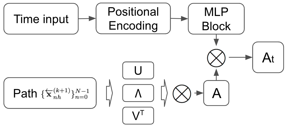
Figure 6: Architecture of the linear module. Both $U$ and $V$ are orthogonal matrices and $\Lambda$ denotes the singular values.

D.2 Synthetic Data

D.2.1 Checkerboard Data

The generation of the checkerboard data is presented in Figure. 7. The probability path is presented in Figure. 8. The conclusion is similar to the spiral data.

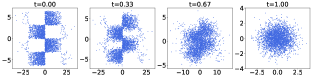
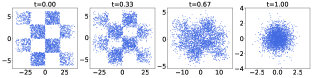
Figure 7: Variational Schrödinger diffusion models (VSDMs, right) v.s. SGMs (left) with the same hyperparameters ($\beta_{\max}=10$).

(a) SGM-10

(b) SGM-20

(c) SGM-30

(d) VSDM-10

Figure 8: Probability flow ODE via VSDMs and SGMs. SGM with $\beta_{\max}=10$ is denoted by SGM-10 for convenience.

D.2.2 Convergence and Computational Time

Convergence Study

Under the same setup, VSDM-10 adaptively learns ${\mathrm{\mathbf{A}}}_{t}$ (and ${\bf D}_{t}$) on the fly and adapts through the pathological geometry via optimal transport. For the spiral-8Y data, the Y-axis of the singular values of ${\bf D}_{t}$ (scaled by $\beta_{\max}$) converges from 10 to around 19 as shown in Figure 9. The singular value of the X-axis quickly converges from 10 to a conservative scale of 7. We also tried VSDM-20 and found that both the Y-axis and X-axis converge to similar scales, which justifies the stability.

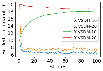
(a) Spiral-8Y

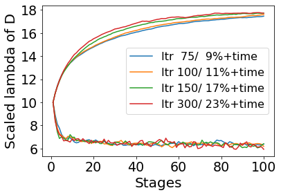
(b) Convergence v.s. time

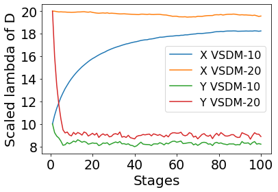
(c) Checkboard-6X

Figure 9: Optimization of ${\boldsymbol{\Lambda}}$ of ${\bf D}$ scaled by $\beta_{\max}$ (scaled lambda of ${\bf D}$) of VSDM-10 and VSDM-20.

Computational Time

We tried different budgets to train the variational scores and observed in Figure 9(b) that 300 iterations yield the fastest convergence among the 4 choices but also lead to 23% extra time compared to SGM. Reducing the number of iterations impacts convergence minimally due to the linearity of the variational scores and significantly reduces the training time.

D.2.3 Evaluation of The Straightness

Straighter trajectories lead to a smaller number of functional evaluations (NFEs). In section D.2.3, we compare VSDM-20 with SGM-20 with NFE=6 and NFE=8 using the same computational budget and observe in Figure 10 and 11 the superiority of the VSDM model in generating more details.

To evaluate the straightness of the probability flow ODE, similar in spirit to Pooladian et al. (2023), we define our straightness metric by approximating the second derivative of the probability flow (18) as follows

$$\begin{split}\text{S}(i)&=\int_{0}^{T}\mathbb{E}_{\overleftarrow{{\bf x}}_{t}\sim\overleftarrow{\rho}_{t}}\bigg{[}\bigg{|}\frac{\mathrm{d}^{2}\overleftarrow{{\bf x}}_{t}(i)}{\mathrm{d}t^{2}}\bigg{|}\bigg{]}\mathrm{d}t,\\ \end{split}$$ (38)

where $i\in\{1,2\}$, $\overleftarrow{{\bf x}}_{t}(1)$ and $\overleftarrow{{\bf x}}_{t}(2)$ denote the X-axis and Y-axis, respectively. $S\geq 0$ and $S=0$ only when the transport is a straight path.

We report the straightness in Table 4 and find the improvement of VSDM-10 over SGM-20 and SGM-30 is around 40%. We also tried VSDM-20 on both datasets and found a significant improvement over the baseline SGM methods. However, despite the consistent convergence in Figure 9, we found VSDM-20 still performs slightly worse than VSDM-10, which implies the potential to tune $\beta_{\max}$ to further enhance the performance.

Table 4: Straightness metric defined in Eq.(38) via SGMs and VSDM with different $\beta_{\max}$’s. SGM with $\beta_{\max}=10$ (SGM-10) fails to generate data of anisotropic shapes and is not reported.

Straightness (X / Y)	Spiral-8Y	Checkerboard-6X
SGM-20	8.3 / 49.3	53.5 / 11.0
SGM-30	9.4 / 57.3	64.6 / 13.1
VSDM-20	6.3 / 45.6	49.4 /    7.4
VSDM-10	5.5 / 38.7	43.9 /    6.5

D.2.4 A Smaller Number of Function Evaluations

We also compare our VSDM-20 with SGM-20 based on a small number of function evaluations (NFE). We use probability flow to conduct the experiments and choose a uniform time grid for convenience. We find that both models cannot fully generate the desired data with NFE=6 in Figure 10 and VSDM appears to recover more details, especially on the top and bottom of the spiral. For the checkboard data, both models work nicely under the same setting and we cannot see a visual difference. With NFE=8 in Figure 11, we observe that our VSDM-20 works remarkably well on both datasets and is slightly superior to SGM-20 in generating the corner details.

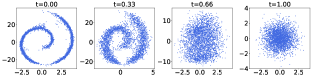
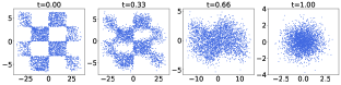
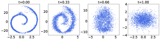
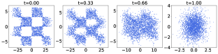
Figure 10: Variational Schrödinger diffusion models (bottom) v.s. SGMs (top) with the same hyperparameters ($\beta_{\max}=20$) and six function evaluations (NFE=6). Both models are generated by probability flow ODE.

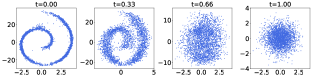
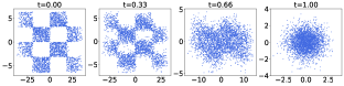
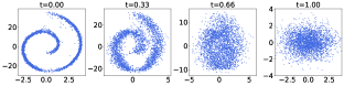
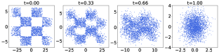
Figure 11: Variational Schrödinger diffusion models (bottom) v.s. SGMs (top) with the same hyperparameters ($\beta_{\max}=20$) and eight function evaluations (NFE=8). Both models are generated by probability flow ODE.

D.3 Multivariate Probabilistic Forecasting

Data.

We use publicly available datasets. Exchange rate has 6071 8-dimensional measurements and a daily frequency. The goal is to predict the value over the next 30 days. Solar is an hourly 137-dimensional dataset with 7009 values. Electricity is also hourly, with 370 dimensions and 5833 measurements. For both, we predict the values over the next day.

Training.

We adopt the encoder-decoder architecture as described in the main text, and change the decoder to either our generative model or one of the competitors. The encoder is an LSTM with 2 layers and a hidden dimension size 64. We train the model for 200 epochs, where each epoch takes 50 model updates. In case of our model we also alternate between two training directions at a predefined rate. The neural network parameterizing the backward direction has the same hyperparameters as in (Rasul et al., 2021), that is, it has 8 layers, 8 channels, and a hidden dimension of 64. The DDPM baseline uses a standard setting for the linear beta-scheduler: $\beta_{\text{min}}=0.0001$, $\beta_{\text{max}}=0.1$ and 150 steps.

References

• Albergo & Vanden-Eijnden (2023) Albergo, M. S. and Vanden-Eijnden, E. Building Normalizing Flows with Stochastic Interpolants. In International Conference on Learning Representation (ICLR), 2023.
• Albergo et al. (2023) Albergo, M. S., Bof, N. M., and Vanden-Eijnden, E. Stochastic Interpolants: A Unifying Framework for Flows and Diffusions. arXiv:2303.08797v1, pp.  1–48, 2023.
• Anderson (1982) Anderson, B. D. Reverse-time Diffusion Equation Models. Stochastic Processes and Their Applications, 12(3):313–326, 1982.
• Ansari et al. (2020) Ansari, A. F., Ang, M. L., and Soh, H. Refining Deep Generative Models via Discriminator Gradient Flow. In International Conference on Learning Representations, 2020.
• Benveniste et al. (1990) Benveniste, A., Métivier, M., and Priouret, P. Adaptive Algorithms and Stochastic Approximations. Berlin: Springer, 1990.
• Blei et al. (2017) Blei, D. M., Kucukelbir, A., and McAuliffe, J. D. Variational Inference: A Review for Statisticians. Journal of the American Statistical Association, 112 (518), 2017.
• Bunne et al. (2023) Bunne, C., Hsieh, Y.-P., Cuturi, m., and Krause, A. The Schrödinger Bridge between Gaussian Measures has a Closed Form. In AISTATS, 2023.
• Caluya & Halder (2022) Caluya, K. F. and Halder, A. Wasserstein Proximal Algorithms for the Schrödinger Bridge Problem: Density Control with Nonlinear Drift. IEEE Transactions on Automatic Control, 67(3):1163–1178, 2022.
• Chan et al. (2022) Chan, A., Silva, H., Lim, S., Kozuno, T., Mahmood, A. R., and White, M. Greedification Operators for Policy Optimization: Investigating Forward and Reverse KL Divergences. Journal of Machine Learning Research, 2022.
• Chen et al. (2023a) Chen, H., Lee, H., and Lu, J. Improved Analysis of Score-based Generative Modeling: User-friendly Bounds under Minimal Smoothness Assumptions. In International Conference on Machine Learning, pp. 4735–4763, 2023a.
• Chen et al. (2022a) Chen, S., Chewi, S., Li, J., Li, Y., Salim, A., and Zhang, A. R. Sampling is as Easy as Learning the Score: Theory for Diffusion Models with Minimal Data Assumptions. arXiv preprint arXiv:2209.11215v2, 2022a.
• Chen et al. (2022b) Chen, T., Liu, G.-H., and Theodorou, E. A. Likelihood Training of Schrödinger Bridge using Forward-Backward SDEs Theory. In International Conference on Learning Representation (ICLR), 2022b.
• Chen et al. (2023b) Chen, T., Gu, J., Dinh, L., Theodorou, E. A., Susskind, J., and Zhai, S. Generative Modeling with Phase Stochastic Bridges. In arXiv:2310.07805v2, 2023b.
• Chen & Georgiou (2016) Chen, Y. and Georgiou, T. Stochastic Bridges of Linear Systems. IEEE Transactions on Automatic Control, 61(2), 2016.
• Chen et al. (2021) Chen, Y., Georgiou, T. T., and Pavon, M. Stochastic Control Liaisons: Richard Sinkhorn Meets Gaspard Monge on a Schrödinger Bridge. SIAM Review, 63(2):249–313, 2021.
• Chen et al. (2023c) Chen, Y., Deng, W., Fang, S., Li, F., Yang, N., Zhang, Y., Rasul, K., Zhe, S., Schneider, A., and Nevmyvaka, Y. Provably Convergent Schrödinger Bridge with Applications to Probabilistic Time Series Imputation. In ICML, 2023c.
• Chewi (2023) Chewi, S. Log-Concave Sampling. online draft, 2023.
• De Bortoli et al. (2021) De Bortoli, V., Thornton, J., Heng, J., and Doucet, A. Diffusion Schrödinger Bridge with Applications to Score-Based Generative Modeling. In Advances in Neural Information Processing Systems (NeurIPS), 2021.
• Deng et al. (2024) Deng, W., Chen, Y., Yang, N., Du, H., Feng, Q., and Chen, R. T. Q. Reflected Schrödinger Bridge for Constrained Generative Modeling. In Conference on Uncertainty in Artificial Intelligence (UAI), 2024.
• Dhariwal & Nichol (2022) Dhariwal, P. and Nichol, A. Diffusion Models Beat GANs on Image Synthesis. In Advances in Neural Information Processing Systems (NeurIPS), 2022.
• Dockhorn et al. (2022) Dockhorn, T., Vahdat, A., and Kreis, K. Score-Based Generative Modeling with Critically-Damped Langevin Diffusion. In International Conference on Learning Representation (ICLR), 2022.
• Finlay et al. (2020) Finlay, C., Jacobsen, J.-H., Nurbekyan, L., and Oberman, A. How to Train Your Neural ODE: the World of Jacobian and Kinetic Regularization. In ICML, 2020.
• Grathwohl et al. (2019) Grathwohl, W., Chen, R. T. Q., Bettencourt, J., Sutskever, I., and Duvenaud, D. FFJORD: Free-form Continuous Dynamics for Scalable Reversible Generative Models. In International Conference on Learning Representation (ICLR), 2019.
• Heusel et al. (2017) Heusel, M., Ramsauer, H., Unterthiner, T., Nessler, B., and Hochreiter, S. GANs Trained by a Two Time-Scale Update Rule Converge to a Local Nash Equilibrium. In Neural Information Processing Systems, 2017.
• Ho et al. (2020) Ho, J., Jain, A., and Abbeel, P. Denoising Diffusion Probabilistic Models. In Advances in Neural Information Processing Systems (NeurIPS), 2020.
• Ho et al. (2022) Ho, J., Chan, W., Saharia, C., Whang, J., Gao, R., Gritsenko, A., Kingma, D. P., Poole, B., Norouzi, M., Fleet, D. J., and Salimans, T. Imagen Video: High Definition Video Generation with Diffusion Models. In arXiv:2210.02303, 2022.
• Huang et al. (2021) Huang, C.-W., Lim, J. H., and Courville, A. A Variational Perspective on Diffusion-Based Generative Models and Score Matching. In Advances in Neural Information Processing Systems (NeurIPS), 2021.
• Hutchinson (1989) Hutchinson, M. F. A Stochastic Estimator of the Trace of the Influence Matrix for Laplacian Smoothing Splines. Communications in Statistics-Simulation and Computation, 18(3):1059–1076, 1989.
• Hyvärinen (2005) Hyvärinen, A. Estimation of Non-normalized Statistical Models by Score Matching. Journal of Machine Learning Research, 6(24):695–709, 2005.
• Janati et al. (2020) Janati, H., Muzellec, B., Peyré, G., and Cuturi, M. Entropic Optimal Transport between Unbalanced Gaussian Measures has a Closed Form. In Advances in Neural Information Processing Systems (NeurIPS), 2020.
• Karatzas & Shreve (1998) Karatzas, I. and Shreve, S. E. Brownian Motion and Stochastic Calculus. Springer, 1998.
• Karras et al. (2022) Karras, T., Aittala, M., Aila, T., and Laine, S. Elucidating the Design Space of Diffusion-Based Generative Models. In Advances in Neural Information Processing Systems (NeurIPS), 2022.
• Kingma et al. (2021) Kingma, D. P., Salimans, T., Poole, B., and Ho, J. Variational Diffusion Models. ArXiv, abs/2107.00630, 2021.
• Koehler et al. (2023) Koehler, F., Heckett, A., and Risteski, A. Statistical Efficiency of Score Matching: The View from Isoperimetry. In ICLR, 2023.
• Kong et al. (2021) Kong, Z., Ping, W., Huang, J., Zhao, K., and Catanzaro, B. DiffWave: A Versatile Diffusion Model for Audio Synthesis . In Proc. of the International Conference on Learning Representation (ICLR), 2021.
• Kullback (1968) Kullback, S. Probability Densities with Given Marginals. Ann. Math. Statist., 1968.
• Lavenant & Santambrogio (2022) Lavenant, H. and Santambrogio, F. The Flow Map of the Fokker–Planck Equation Does Not Provide Optimal Transport. Applied Mathematics Letters, 133, 2022.
• Lee et al. (2022) Lee, H., Lu, J., and Tan, Y. Convergence for Score-based Generative Modeling with Polynomial Complexity. Advances in Neural Information Processing Systems (NeurIPS), 2022.
• Léonard (2014) Léonard, C. A Survey of the Schrödinger Problem and Some of its Connections with Optimal Transport. Discrete & Continuous Dynamical Systems-A, 34(4):1533–1574, 2014.
• Liang et al. (2007) Liang, F., Liu, C., and Carroll, R. J. Stochastic Approximation in Monte Carlo Computation. Journal of the American Statistical Association, 102:305–320, 2007.
• Lipman et al. (2023) Lipman, Y., Chen, R. T. Q., Ben-Hamu, H., Nickel, M., and Le, M. Flow Matching for Generative Modeling. In Proc. of the International Conference on Learning Representation (ICLR), 2023.
• Liptser & Shiryaev (2001) Liptser, R. S. and Shiryaev, A. N. Statistics of Random Processes: I. General Theory. Springer Science & Business Media, 2001.
• Liu (2022) Liu, Q. Rectified Flow: A Marginal Preserving Approach to Optimal Transport. arXiv:2209.14577, 2022.
• Liu et al. (2023) Liu, X., Gong, C., and Liu, Q. Flow Straight and Fast: Learning to Generate and Transfer Data with Rectified Flow. In International Conference on Learning Representation (ICLR), 2023.
• Lu et al. (2022) Lu, C., Zhou, Y., Bao, F., Chen, J., Li, C., and Zhu, J. DPM-Solver: A Fast ODE Solver for Diffusion Probabilistic Model Sampling in Around 10 Steps. In Advances in Neural Information Processing Systems (NeurIPS), 2022.
• Luo (2023) Luo, W. A Comprehensive Survey on Knowledge Distillation of Diffusion Models. arXiv preprint arXiv:2304.04262, 2023.
• Luo et al. (2024a) Luo, W., Hu, T., Zhang, S., Sun, J., Li, Z., and Zhang, Z. Diff-instruct: A Universal Approach for Transferring Knowledge from Pre-trained Diffusion Models. Advances in Neural Information Processing Systems, 36, 2024a.
• Luo et al. (2024b) Luo, W., Zhang, B., and Zhang, Z. Entropy-based Training Methods for Scalable Neural Implicit Samplers. NeurIPS, 36, 2024b.
• Ma & Yong (2007) Ma, J. and Yong, J. Forward-Backward Stochastic Differential Equations and their Applications. Springer, 2007.
• Marzouk et al. (2016) Marzouk, Y., Moselhy, T., Parno, M., and Spantini, A. Sampling via Measure Transport: An Introduction. Handbook of Uncertainty Quantification, pp.  1–41, 2016.
• McCann (1997) McCann, R. J. A Convexity Principle for Interacting Gases. Advances in mathematics, 128(1):153–179, 1997.
• Øksendal (2003) Øksendal, B. Stochastic Differential Equations: An Introduction with Applications. Springer, 2003.
• Onken et al. (2021) Onken, D., Fung, S. W., Li, X., and Ruthotto, L. OT-Flow: Fast and Accurate Continuous Normalizing Flows via Optimal Transport. In Proc. of the National Conference on Artificial Intelligence (AAAI), 2021.
• Pavon et al. (2021) Pavon, M., Tabak, E. G., and Trigila, G. The Data-driven Schrödinger Bridge. Communications on Pure and Applied Mathematics, 74:1545–1573, 2021.
• Peluchetti (2023) Peluchetti, S. Diffusion Bridge Mixture Transports, Schrödinger Bridge Problems and Generative Modeling. ArXiv e-prints arXiv:2304.00917v1, 2023.
• Peyré & Cuturi (2019) Peyré, G. and Cuturi, M. Computational Optimal Transport: With Applications to Data Science. Foundations and Trends in Machine Learning, 2019.
• Polyak & Juditsky (1992) Polyak, B. T. and Juditsky, A. Acceleration of Stochastic Approximation by Averaging. SIAM Journal on Control and Optimization, 30:838–855, 1992.
• Pooladian et al. (2023) Pooladian, A.-A., Ben-Hamu, H., Domingo-Enrich, C., Amos, B., Lipman, Y., and Chen, R. T. Q. Multisample Flow Matching: Straightening Flows with Minibatch Couplings. In ICML, 2023.
• Ramesh et al. (2022) Ramesh, A., Dhariwal, P., Nichol, A., Chu, C., and Chen, M. Hierarchical Text-Conditional Image Generation with CLIP Latents. In arXiv:2204.06125v1, 2022.
• Rasul et al. (2021) Rasul, K., Seward, C., Schuster, I., and Vollgraf, R. Autoregressive Denoising Diffusion Models for Multivariate Probabilistic Time Series Forecasting. In International Conference on Machine Learning, 2021.
• Robbins & Monro (1951) Robbins, H. and Monro, S. A Stochastic Approximation Method. Annals of Mathematical Statistics, 22:400–407, 1951.
• Ruschendorf (1995) Ruschendorf, L. Convergence of the Iterative Proportional Fitting Procedure. Ann. of Statistics, 1995.
• Salimans & Ho (2022) Salimans, T. and Ho, J. Progressive Distillation for Fast Sampling of Diffusion Models. In ICLR, 2022.
• Salinas et al. (2019) Salinas, D., Bohlke-Schneider, M., Callot, L., Medico, R., and Gasthaus, J. High-dimensional Multivariate Forecasting with Low-rank Gaussian Copula Processes. Advances in neural information processing systems, 2019.
• Särkkä & Solin (2019) Särkkä, S. and Solin, A. Applied Stochastic Differential Equations. Cambridge University Press, 2019.
• Shi et al. (2023) Shi, Y., De Bortoli, V., Campbell, A., and Doucet, A. Diffusion Schrödinger Bridge Matching. In Advances in Neural Information Processing Systems (NeurIPS), 2023.
• Singhal et al. (2023) Singhal, R., Goldstein, M., and Ranganath, R. Where to Diffuse, How to Diffuse, and How to Get Back: Automated Learning for Multivariate Diffusions. In Proc. of the International Conference on Learning Representation (ICLR), 2023.
• Song & Ermon (2020) Song, Y. and Ermon, S. Improved Techniques for Training Score-Based Generative Models. In Advances in Neural Information Processing Systems (NeurIPS), 2020.
• Song et al. (2020) Song, Y., Garg, S., Shi, J., and Ermon, S. Sliced Score Matching: A Scalable Approach to Density and Score Estimation. In Uncertainty in Artificial Intelligence, 2020.
• Song et al. (2021a) Song, Y., Durkan, C., Murray, I., and Ermon, S. Maximum Likelihood Training of Score-Based Diffusion Models . In Advances in Neural Information Processing Systems (NeurIPS), 2021a.
• Song et al. (2021b) Song, Y., Sohl-Dickstein, J., Kingma, D. P., Kumar, A., Ermon, S., and Poole, B. Score-Based Generative Modeling through Stochastic Differential Equations . In International Conference on Learning Representation (ICLR), 2021b.
• Tanaka (2019) Tanaka, A. Discriminator Optimal Transport. In Neural Information Processing Systems, 2019.
• Tong et al. (2023) Tong, A., Malkin, N., Huguet, G., Zhang, Y., Rector-Brooks, J., Fatras, K., Wolf, G., and Bengio, Y. Improving and Generalizing Flow-based Generative Models with Minibatch Optimal Transport. arXiv:2302.00482v3, 2023.
• Trivedi & Kondor (2017) Trivedi, S. and Kondor, R. Optimization for Deep Neural Networks. Slides - University of Chicago, 2017.
• Vahdat et al. (2021) Vahdat, A., Kreis, K., and Kautz, J. Score-based Generative Modeling in Latent Space. Advances in Neural Information Processing Systems, 34:11287–11302, 2021.
• Vanden-Eijnden (2001) Vanden-Eijnden, E. Introduction to Regular Perturbation Theory. Slides, 2001. URL https://cims.nyu.edu/~eve2/reg_pert.pdf.
• Vargas et al. (2021) Vargas, F., Thodoroff, P., Lamacraft, A., and Lawrence, N. Solving Schrödinger Bridges via Maximum Likelihood. Entropy, 23(9):1134, 2021.
• Vempala & Wibisono (2022) Vempala, S. S. and Wibisono, A. Rapid Convergence of the Unadjusted Langevin Algorithm: Isoperimetry Suffices, 2022.
• Villani (2003) Villani, C. Topics in Optimal Transportation, volume 58. American Mathematical Soc., 2003.
• Vono et al. (2022) Vono, M., Paulin, D., and Doucet, A. Efficient MCMC Sampling with Dimension-Free Convergence Rate using ADMM-type Splitting. Journal of Machine Learning Research, 2022.
• Xue et al. (2023) Xue, S., Yi, M., Luo, W., Zhang, S., Sun, J., Li, Z., and Ma, Z.-M. SA-Solver: Stochastic Adams Solver for Fast Sampling of Diffusion Models. Advances in Neural Information Processing Systems, 2023.
• Zhang et al. (2024) Zhang, B., Luo, W., and Zhang, Z. Enhancing Adversarial Robustness via Score-Based Optimization. Advances in Neural Information Processing Systems, 36, 2024.