Predictive Enforcement

Abstract

We study law enforcement guided by data-informed predictions of “hot spots” for likely criminal offenses. Such “predictive” enforcement could lead to data being selectively and disproportionately collected from neighborhoods targeted for enforcement by the prediction. Predictive enforcement that fails to account for this endogenous “datafication” may lead to the over-policing of traditionally high-crime neighborhoods and performs poorly, in particular, in some cases as poorly as if no data were used. Endogenizing the incentives for criminal offenses identifies additional deterrence benefits from the informationally efficient use of data.

Keywords: Data-driven enforcement, one-armed bandit with changing world, hidden Markov-chain, a bandit with endogenously-valued arm

1 Introduction

Data-guided prediction algorithms are becoming increasingly common in law enforcement. Predictive algorithms such as Risk Terrain Modeling, Spatio-Temporal, Near Repeat Modeling, have become standard crime-fighting tools for police departments in major US cities (See Pearsall (2010); Perry, McInnis, Price, Smith, and Hollywood (2013); Brayne (2020)). These algorithms forecast “hot spots” for criminal activity and recommend allocation of enforcement resources accordingly. Credit card companies also use data to flag suspicious transactions, while municipal governments are using data to enforce a multitude of rules and regulations. For example, New York City has a special analytic team that applies big-data analytics to solve problems related to enforcement. One famously-cited anecdote is the inspection of “illegal conversions”—a practice of dividing a dwelling into many smaller units for extra rental income; they are major fire hazards, among other issues. By linking numerous data and using them to predict the likely violations and the severity of fire hazards, the team was able to steer its 200 inspectors to select among 25,000 complaints received each year, leading to a five-fold improvement in the effectiveness of its inspection.

While there are many success stories of predictive enforcement, there are also criticisms. Critics argue that prediction algorithms are often unreliable and tend to over-police certain communities, particularly non-white and low-income groups. They claim that these algorithms are trained on biased data that reflects historical biases made by humans, perpetuating these biases. Additionally, a positive feedback loop between enforcement and crime detection can arise: concentrating police patrol on a high-crime neighborhoods leads to more arrests being made and more crimes being detected in that neighborhood, leading to further concentration of police patrol in those neighborhoods and perpetuating the cycle.

In this paper, we develop a theoretical framework for understanding predictive enforcement, with a focus on the endogenous nature of data collection or “datafication.” Crime data is rarely random or representative, but rather a result of past enforcement and surveillance activities. The feedback loop between enforcement and information gathering is a crucial feature of this framework, particularly for so-called “victimless crimes” such as drugs, gambling, and prostitution, the detection of which requires enforcement/surveillance by the police.

To capture the link between enforcement and data collection, we adopt a bandit model. At each time $t\in(-\infty,\infty)$, a policymaker (PM) allocates $y_{t}\in[0,1]$ of enforcement resources (such as police patrol units) to a single neighborhood at (flow) marginal cost $c>0$. The “neighborhood” is a metaphor for any observable characteristics such as geographic locations, groups of individuals, types of credit card transactions, and types of housing (in the context of illegal conversions) that PM may target for enforcement. The “cost” reflects the opportunity cost of diverting enforcement resources away from other neighborhoods or covariates.

Given allocation $y_{t}$, a crime attempted at $t$ is intervened in, and harm is avoided, with probability $y_{t}$. Whether a crime is attempted in the neighborhood depends on its underlying crime condition, which we model as the arrival of a crime opportunity. The arrival rate of crime opportunities, denoted by $\tilde{\lambda}$, is random and depends on the underlying state: $\tilde{\lambda}$ equals $\lambda>0$ in state $H$ (or “high crime”) and 0 in state $L$ (“safe”). The unknown state constitutes the main uncertainty faced by the PM, and the crime data generated by past enforcement can help resolve this uncertainty.

Our model is similar to that of Keller, Rady, and Cripps (2005) (henceforth, KRC), but we depart from KRC in two crucial ways. First, unlike KRC, the state is not fixed but rather changes according to a continuous-time Markov chain with a long-run probability $\pi_{0}$ that the state is $H$. We adopt this “changing world” model for two reasons. Firstly, criminal conditions, as represented by $\tilde{\lambda}$, are often not fixed but rather change stochastically over time. Various factors such as foot traffic, weather conditions, and socioeconomic variables, can influence the susceptibility of a neighborhood to crimes, and these factors change over time in a way not entirely captured by observed data. Secondly, the “changing world” serves a crucial analytical purpose. With a fixed state, the PM will eventually learn the true state, so the value of learning is transient and short-lived. However, with the changing world, the need for learning never vanishes, allowing us to study the value of learning, which is the crucial element of predictive enforcement, even in the long run.

In addition to the exogenous crime opportunities, the commission of crime in our model also depends on the criminal’s incentives, which are endogenously determined by the expected enforcement decision. In the second part of our model, we endogenize crime activity by analyzing the incentives of the criminals. This feature makes the value of the “arm” endogenously dependent on the likelihood of that arm being chosen. Analytically, this means that the value of enforcement resources allocated to a particular neighborhood depends not only on the underlying crime condition but also on the incentives of the criminals, which are in turn influenced by the expected enforcement decision.

In our study, we analyze the optimal predictive (OP) policy under two environments, each taking into consideration the link between enforcement and information collection. We compare OP against two benchmarks: (i) the non-predictive (NP) policy, which does not use past crime data for enforcement decisions, and (ii) the greedy predictive (GP) policy, which uses the prediction but ignores its implications for datafication by only using it for enforcement in a myopically optimal way. We view these benchmarks as representing the traditional and current approaches to predictive enforcement, respectively. Specifically, GP aligns well with the standard account of predictive enforcement being adopted in practice, where the prediction is used to achieve immediate enforcement goals without considering the future implications for data collection.

Our results can be summarized as follows. First, we consider the case of exogenous crime, where a potential criminal commits a crime with a fixed probability $x\in(0,1]$ upon receiving a crime opportunity, and the social loss of an unintervened-in/unmitigated crime is $1. Under the non-predictive (NP) policy, the PM chooses optimal enforcement policy without consulting crime data, so she chooses $y_{t}=1$ for all $t$ if the long-run crime rate $x\lambda\pi_{0}$ [i.e., evaluated at the long-run prior $\pi_{0}$] exceeds the per-unit cost $c$, or if the long-run prior $\pi_{0}$ exceeds the myopic cutoff, $\hat{p}_{M}:=c/x\lambda$, and she chooses $y_{t}=0$ if $\pi_{0}<\hat{p}_{M}$. In particular, if the alternative neighborhood is traditionally crime-prone, the opportunity cost, or the myopic cutoff, will be high, and the policy will call for no enforcement of the reference neighborhood.

In both the greedy predictive (GP) and optimal predictive (OP) policies, the PM forms her posterior belief $p$ on the state based on the crime data, specifically the timing of the last detected crime, and adjusts her enforcement level based on that belief. Under GP, the PM follows a cutoff policy with the myopic cutoff $\hat{p}_{M}$ as a threshold: $y(p)=1$ if $p>\hat{p}_{M}$ and $y(p)=0$ if $p<\hat{p}_{M}$. The OP also has a cutoff structure but its cutoff $\hat{p}$ may not coincide with the myopic cutoff $\hat{p}_{M}$. The cutoff level $\hat{p}$ depends on the opportunity cost of enforcement $c$. If the cost is sufficiently high, then the cutoff is so high that OP eventually calls for no enforcement. If the cost is sufficiently low, then the cutoff is so low that OP eventually calls for full enforcement. In these two cases, NP and GP lead to the same long-run outcome as OP. Intuitively, when the cost is too high or too low, there is little uncertainty about the optimal policy, so prediction has no value.

When the cost is at an intermediate level, prediction is potentially valuable, and its use for enforcement decisions matters. In this case, the optimal cutoff $\hat{p}$ is set strictly below the myopic cutoff $\hat{p}_{M}$ to allow for more exploration than GP, which focuses only on exploitation. Hence, when GP departs from OP, the former enforces too little relative to OP. In fact, GP departs from OP when the opportunity cost $c$ tends to be either high or intermediate, i.e., when the alternative neighborhoods are traditionally crime-prone. This result is consistent with the complaint that predictive enforcement over-polices past high-crime neighborhoods. Note that this result is obtained without any systemic bias in the prediction against such neighborhoods and is attributed entirely to an insufficient exploration on the part of GP.

Is predictive enforcement effective? The answer depends on how prediction is used for the enforcement decision. If the PM can learn only from enforcement, as is assumed in the baseline model, GP does not perform better than NP in the long run, despite the fact that GP makes use of prediction whereas NP does not. This result echoes the complaint about its lack of reliability in current predictive enforcement practices. It suggests that prediction can have no value unless the PM uses it informationally optimally. It also suggests that the feedback loop between enforcement and exploration is responsible for the poor performance of the myopically optimal use of prediction.

More generally, GP does better than NP if the PM can also learn without enforcement, for example, from community reporting of crimes. Its performance converges to that of NP in payoff as the background learning vanishes and to that of OP if the background learning becomes so effective that enforcement yields no extra learning.

In Section 4, we endogenize the crime rate through the potential criminal’s incentives to commit a crime. We assume that there exists a critical enforcement level $\hat{y}\in(0,1)$ such that a criminal will commit a crime with probability $x=1$ if he expects the enforcement level to be $y>\hat{y}$, and with probability $x=0$ if he expects $y<\hat{y}$, and with any probability $x\in[0,1]$ if he expects $y=\hat{y}$. We also assume that potential criminals are non-predictive, meaning they do not have access to the crime data, so their crime decision can only depend on their prior expected enforcement rate. We then look for a Markov perfect equilibrium where the strategy of the PM may only depend on $p$, the belief about the state being $H$.

Under NP, neither criminal’s strategy nor the PM’s strategy depends on the prediction $p$ informed by the crime data. What ensues then is the classic inspection game: both PM and criminals randomize if $c$ is not too large. PM chooses an interior enforcement level $y=\hat{y}$ that keeps the criminals indifferent, and criminals choose an interior crime probability $\hat{x}=c/(\lambda\pi_{0})$ that keeps the PM indifferent with regard to her enforcement.

Under GP and NP, the PM’s strategies must form the best responses against the equilibrium crime behavior chosen by potential criminals. Therefore, the PM’s strategies under these regimes follow the characterizations in the exogenous crime case, given the criminals’ behavior (which is now endogenous). Recall that, holding the crime rate fixed, the PM is willing to enforce more under OP than under GP. This feature makes enforcement more credible and generates more deterrence under OP than under GP, resulting in a lower crime rate under OP than under GP in equilibrium. When $c$ is sufficiently small, GP and OP prescribe the same cutoff policy, making them observationally equivalent. However, the crime rate is lower under OP than under GP.

Finally, we consider the possibility of the criminals accessing the crime data and harnessing the same predictive power as the PM. The GP and OP then entail the outcome of the inspection game equilibrium for each prediction about the state. This gives rise to a three-way tie across the alternative regimes. This limit benchmark illustrates that the value of prediction hinges on the PM having an upper hand in the predictive “arms race,” which may vanish as the superiority PM enjoys in her prediction power erodes.

Related Literature.

The current paper is part of the enforcement literature initiated by by Becker (1968), and the inspection games that studies the equilibrium interplay between an enforcer and an enforced, Our model considers a dynamic version of these models. Several recent papers consider dynamic inspection models studying optimal frequency of inspection; see Dilmé and Garrett (2019), Varas, Marinovic, and Skrzypacz (2020); Wagner and Knoepfle (2021); Ball and Knoepfle (2023). The current paper differs in its focus on the endogenous datafication process through a bandit framework. In particular, the current model can be seen as generalizing the planner’s problem in Keller, Rady, and Cripps (2005) by introducing a “changing world” and by introducing an endogenously-valued arm. Endogenous datafication is also featured in different contexts by Che and Hörner (2018) and Che, Kim, and Zhong (2020).

Ichihashi (2023) studies predictive policing from the information design perspective. He finds that suppressing information about criminals’ types leads to a more efficient allocation of enforcement resources and thus more effective deterrence. His model does not consider the dynamic feedback between enforcement and information acquisition, the main focus of the current paper. Lum and Isaac (2016) and Ensign, Friedler, Neville, Scheidegger, and Venkatasubramanian (2018) consider the dynamic feedback and point out the possible mis-inference and mis-prediction of true crime activities. The PM in our model is fully Bayesian and avoids such inference errors. Mohler, Short, Malinowski, Johnson, Tita, Bertozzi, and Brantingham (2015) study the performance of PredPol algorithm, a leading predictive policy algorithm deployed by several police departments. Remarkably, the predictive policies, OP and GP, in our model match the qualitative feature of the PredPol algorithm, namely the “earthquake model,” which predicts the crime rate to decay exponentially as time progresses without experiencing another crime incidence. In our model, this feature arises from the Bayesian updating about underlying changing state, whereas the PredPol model assumes this feature directly through a self-exciting point process.

The current paper also intersects with the literature on racial profiling and the recent literature on algorithmic fairness. We do not consider fairness as part of the PM’s objective in our analysis. Rather, we draw fairness implications of the failure to account for endogenous datafication.

2 Preliminaries

2.1 Setup

A “neighborhood” that has a unit mass of potential “criminals.” These labels should be interpreted generally: criminals are potential violators of any law, safety, health regulations, city ordinance, zoning, and housing code, and not just those who may commit violent crimes, and a neighborhood means any observable characteristics such as a geographic location, types of financial transactions, and types of regulated housing units, that the enforcement authority, we call policymaker (PM), may track and target for intervention.

The time is continuous with $t\in(-\infty,\infty)$. At each point $t$ in time, crime opportunity arrives to an individual in the neighborhood at an uncertain Poisson rate $\tilde{\lambda}$ that depends on the state of the world, or simply “state.” The state $\omega_{t}$ could be either “high” ($\omega_{t}=H$) interpreted as crime-susceptible, or “low” ($\omega_{t}=L$) interpreted as safe. In state $\omega_{t}=L$, $\tilde{\lambda}=0$, so no opportunity for crime exists. In state $\omega_{t}=H$ an individual receives a crime opportunity at the rate of $\lambda>0$.

The state is not fixed but rather follows a continuous-time Markov chain. Specifically, state $\omega_{t}=L$ switches to $\omega_{t}=H$ at rate $\rho_{L}>0$ and state $\omega_{t}=H$ switches to $\omega_{t}=L$ at rate $\rho_{H}>0$.

The stationary probability of the state being $\omega_{t}=H$ is then:

$$\pi_{0}:=\frac{\rho_{L}}{\rho_{H}+\rho_{L}}.$$

A useful interpretation/observation is that $\pi_{0}$ is the long-run average fraction of the time that the world is in state $\omega_{t}=H$.

Upon receiving the crime opportunity, the individual commits a crime with probability $x>0$. From now on, we simply call $x$ the crime level. In the sequel, we consider two different scenarios. In the case of exogenous crime, the crime level is fixed. In the case of endogenous crime, the crime level depends on the individual’s incentive, which in turn depends on the expected level of enforcement by PM. We will later model this dependence. We begin with the former both for analytical clarity as well as realism: this assumption approximates the situation in which the elasticity of the crime level to actual enforcement is rather low.

At each time $t$, PM chooses a level of enforcement $y_{t}\in[0,1]$ at cost $c>0$ per unit enforcement. One can interpret $c$ as the direct (say monetary) cost of increasing enforcement, e.g., hiring inspectors/police personnel or equipment. Alternatively, the cost can be interpreted as the opportunity cost of diverting enforcement resources away from other neighborhoods under the PM’s jurisdiction. Indeed, it is useful to flesh out this interpretation.

Two neighborhood model.

Suppose there are two neighborhoods: neighborhood $A$ is one mentioned above with a uncertain crime condition, and neighborhood $B$ is the other neighborhood under the PM’s jurisdiction. Neighborhood $B$ has a known crime condition; crime opportunity arrives to an individual in $B$ at a known rate $\lambda_{B}\in(0,\lambda)$. If $\lambda_{B}>\pi_{0}\lambda$, one might characterize $B$ as a traditionally “high-crime” area. The PM allocates a unit budget of resource allocation at zero cost between the two neighborhoods. A high $\lambda_{B}$ means a high opportunity cost from pulling resources away from $B$, so it corresponds to a high $c$ in our model. Given this mapping, our results translate into the two-neighborhood model. The reader should keep two neighborhood model in mind, as it facilitates interpreting our results with regard to how the policy treats a traditionally high-crime neighborhood. ∎

The PM never directly observes the state $\omega_{t}$, and we let $p_{t}$ denote the PM’s belief that the state is $\omega_{t}=H$ at time $t$. The enforcement serves two functions. Specifically, suppose PM chooses $y_{t}$ at any time $t\geq 0$. Then, it incurs a flow cost $cy_{t}$ at that instant. But, if the crime is attempted at that point, with probability $y_{t}$ the PM

1. intervenes in the crime and mitigates its harm; mitigation can involve either foiling a crime or arresting a criminal after the crime.

2. learns that the state is $\omega_{t}=H$ (since this crime can only be attempted in state $H$).

We assume that unmitigated harm costs $1 to society. Both functions of enforcement accord well with the common practice of law and regulatory enforcement. The primary roles of inspectors are to both redress violations and mitigate the associated harms and to collect information about crime conditions for future predictions. In particular, the information collection role of enforcement is growing in prominence in recent years in the context of predictive policing.

PM’s payoff.

The PM’s payoff is given by the losses she incurs on the infinite horizon. The loss arises from two sources: the unmitigated harm and the cost of enforcement. Suppose that at each time $t$ the state is $\omega_{t}=H$ with probability $p_{t}$, PM chooses an enforcement level $y_{t}$, and the crime probability (given the opportunity) is $x$. Then, PM’s flow loss at $t$ is

$$p_{t}\lambda x(1-y_{t})+cy_{t},$$

so her (discounted) total loss is

$$\int_{0}^{\infty}(p_{t}\lambda x(1-y_{t})+cy_{t})e^{-rt}dt,$$

where $r>0$ is PM’s discounted rate. We assume that $\lambda x>c$ since otherwise, it would be trivially optimal to set $y_{t}=0$ always.

Prediction.

Predictive enforcement utilizes the prediction of future crime based on the observed history of past crimes. In our model, this boils down to forming a posterior belief $p$ based on the detected incidences of crimes. We now formalize the law of motion that governs the belief updating. To see how the belief evolves, suppose a crime is detected at any point. Then, the posterior belief jumps to 1 since crime can only occur in $\omega_{t}=H$. If no crime is detected, then either the state is $\omega_{t}=L$ or $\omega_{t}=H$ but either crime has not occurred or has not been detected. Bayes rule suggests that

$$p_{t+dt}= \frac{p_{t}(1-\rho_{H}dt)(1-\lambda xydt)+(1-p_{t})\rho_{L}dt(1-\lambda xydt)}{p_{t}(1-\rho_{H}dt)(1-\lambda xydt)+(1-p_{t})(1-\rho_{L}dt)+(1-p_{t})\rho_{L}dt(1-\lambda xydt)+p_{t}\rho_{H}dt}+o(dt)$$

$$= \frac{p_{t}(1-\rho_{H}dt-\lambda xydt)+(1-p_{t})\rho_{L}dt}{1-p_{t}\lambda xydt}+o(dt).$$

Hence,

$$\frac{p_{t+dt}-p_{t}}{dt}=\frac{\rho_{L}(1-p_{t})-\rho_{H}p_{t}-p_{t}(1-p_{t})\lambda xy}{1-p_{t}\lambda xdt}+O(dt),$$

so

$$\dot{p}=\underbrace{\rho_{L}(1-p)-\rho_{H}p}_{\mbox{{\color[rgb]{0.703125,0.10546875,0.10546875} \tiny natural rate}}}\underbrace{-\,\,p(1-p)\lambda xy}_{\mbox{{\color[rgb]{0.703125,0.10546875,0.10546875} \tiny updating from ``no detection''}}}=:f(p,y).$$ (1)

It is instructive to unpack the rate at which PM’s belief changes. There are two terms. The first term, $\rho_{L}(1-p)-\rho_{H}p$, is the “natural rate” due to the underlying Markov chain governing the state of the world. If the PM (policymaker) chooses $y_{t}=0$, there is no way to learn the state, so PM’s belief simply follows the natural rate. Naturally, if her prior is $p_{t}>\pi_{0}$, then the belief drifts down toward $\pi_{0}$, and if $p_{t}<\pi_{0}$, then the belief drifts up toward $\pi_{0}$ over time.

If the PM chooses some enforcement $y_{t}>0$, however, then she expects to detect state $\omega_{t}=H$ (assuming $x>0$) occasionally. Not detecting any crime (even with enforcement) then pushes her posterior toward state $\omega_{t}=L$. The second term captures this downward pressure that “tampers” with the natural rate. In particular, the downward pressure is strongest when $y_{t}=1$. Let $\pi_{1}$ be such that $f(\pi_{1},1)=0$. Then, if PM chooses $y_{t}=1$ always, her belief drifts down for $p_{t}>\pi_{1}$ and drifts up for $p_{t}<\pi_{1}$, as long as enforcement yields no detection of crime. Not surprisingly, $\pi_{1}<\pi_{0}$. The belief dynamics is depicted in Figure 1.

Figure 1: PM’s belief updating given no detection.

Given no detection, PM’s belief drifts up if $p_{t}<\pi_{1}$ and drifts down if $p>\pi_{0}$. How the belief evolves within $p_{t}\in(\pi_{1},\pi_{0})$ depends on $y$. In general, the higher $y_{t}$ is, the belief will settle closer toward $\pi_{1}$, absent any jump.

Remark 1 (Fixed state model).

In the KRC bandit model, the state is non-changing, so the natural rate is absent, and the only the second term is active. Hence, the belief in case of “no news” always drifts down and tends to 0 if no crime is detected. This is not the case in our model with changing world: the belief can never permanently fall below $\pi_{1}$ and never permanently stay above $\pi_{0}$.

Admissibility.

Throughout, we will focus on the Markovian strategy by the PM that depends on the payoff-relevant state $p_{t}$. As is clear, this is without a loss for the exogenous crime case and natural for the endogenous crime case. Hence, we often suppress the dependence on the calendar time $t$. Obviously, the law of motion 1 must be well defined along such a strategy. This imposes an admissibility restriction on the strategy $p\mapsto y(p)$. Admissibility will not be an issue for most the part except for the following situation. Suppose $p$ is such that $f(p^{\prime},y(p^{\prime}))>0$ for all $p^{\prime}>p$ (close to $p$ say) and $f(p^{\prime\prime},y(p^{\prime\prime}))<0$ for all $p^{\prime\prime}<p$ (close to $p)$. In this case, admissibility requires that $y(p)=z(p)$, where $z(p)$ satisfies $0=f(p,z(p))=\dot{p}$. This simply means that a belief $p$ must be stationary if it attracts drifts from opposite directions since in that case $p$ must be an absorbing state. Suppose this condition is violated, say $f(p,y(p))<0$. Then, the law of motion is not well-defined at $p$ since the strategy calls for arbitrarily frequent movement back and forth between $p$ and arbitrarily lower belief. Admissibility will play some role in our enforcement policies below, and more discussion will follow on its economic content. Importantly, although admissibility may appear to be a technical condition, it does capture a substantive property of a dynamic system. If one considers a discrete-time approximation of our continuous time model, then the absorbing state corresponds to frequent switching between $y(p^{\prime\prime})=1$ for $p^{\prime\prime}>p$ and $y(p^{\prime})=0$ for $p^{\prime}<p$, and the stationarity-inducing policy $z(p)\in(0,1)$ approximates the fraction of time that $y=1$ is chosen while the system is in the neighborhood of $p$.

2.2 Alternative enforcement regimes

We consider the three plausible scenarios in terms of whether and how data is used to inform PM’s enforcement decision. To what extent each of these scenarios corresponds to real-world practice is debatable. Nevertheless, they will serve as three useful benchmarks that facilitate our understanding of the value and the implications of using data.

Non-predictive enforcement (NP).

As a benchmark for a situation in which crime data is not used to inform the enforcement policy, we assume that the PM never updates her belief about the likelihood of crime based on the crime data. Since such a PM would never learn from past history, her enforcement policy $y$ will be constant in $p$, depending only on her prior. We assume that the prior matches the fundamental ground truth, namely, the long-run rate of crime, $\pi_{0}\lambda x$. Such a prior may be formed based on the PM’s long-term memory or aggregate past crime record.

Given such a prior, the optimal non-predictive enforcement policy is to enforce fully if and only if $\pi_{0}\lambda x\geq c$. More formally, we define the non-predictive enforcement policy to be:

$$y_{\text{\tiny NP}}(p)=\left\{\begin{array}[]{ll}1&\text{for }\pi_{0}>\hat{p}_{M}\\ 0&\text{for }\pi_{0}<\hat{p}_{M},\\ \end{array}\right.$$ (2)

where $\hat{p}_{M}:=c/(\lambda x)$ is the myopic cutoff. Note that $y_{\text{\tiny NP}}(p)$ is a constant function taking either 0 or 1.

Greedy predictive enforcement (GP).

We next consider a benchmark in which the PM updated the posterior $p$ accurately based on the crime history but acts myopically on her enforcement decision, without taking into consideration the informational value of enforcement. This scenario accurately describes the standard practice of predictive enforcement. What data-driven enforcement does is to predict the likelihood of crime at each time and make an optimal decision for that time. We assume that the PM chooses the myopically optimal enforcement decision:

$$y_{\text{\tiny GP}}(p)=\left\{\begin{array}[]{ll}1&\text{for }p>\hat{p}_{M}\\ 0&\text{for }p<\hat{p}_{M},\\ \end{array}\right.$$ (3)

where $p$ is updated according to 1. Note that the PM here uses the full force of prediction afforded by the crime data. Where GP may fall short of its failure to account for the informational value of her enforcement decision.

Again, the greedy nature of GP is consistent with the current enforcement practice, which makes no reference to the informational value of enforcement.

Optimal predictive enforcement (OP).

This regime captures the ideal situation in which PM makes her enforcement choice in a dynamically optimal manner. This means that, just as in GP, the PM forms her posterior $p_{t}$ accurately from the crime data, but she uses that prediction to make an enforcement decision that is long-term optimal, i.e., one that takes into account the informational value of the enforcement decision.

In what follows, the NP and GP will serve as benchmarks against OP. It is important to note that the point of the comparison will not to establish the superiority of OP relative to these benchmarks. These benchmarks are defined to “turn off” some aspect of decision-making that is relevant for the optimal policy, so their inferiority is unsurprising. Rather, the aim is to understand the roles played by the turned-off elements in shaping the optimal policy and to decompose and account for the values that they will contribute toward the optimal policy.

3 Exogenous Crime

In this section, we assume that the crime probability is fixed exogenously at some level $x\in(0,1]$. We first analyze OP and will compare its outcome with those of NP and GP.

3.1 Optimal Predictive Enforcement

The decision problem facing the PM does not depend on the calendar time, depending only on the belief $p$. Hence, the problem reduces to a Markov Decision Problem (MDP) with state variable $p$, and the optimal policy rule is given by $p\mapsto y(p)$, and the subscript $t$ is dropped henceforth. We employ a dynamic programming technique to characterize the optimal policy.

To this end, let $L_{y}(p)$ denote the total discounted loss of PM with belief $p_{t}=p$ who chooses any enforcement policy $y:[0,1]\to[0,1]$. For a short duration $dt>0$, we can write

$$L_{y}(p)=\big{[}p\lambda x(1-y(p))+cy(p)\big{]}dt +p\lambda xy(p)dt(1-rdt)L_{y}(1)$$

$$+(1-rdt)(1-p\lambda xy(p)dt)L_{y}(p_{t+dt})+o(dt).$$

The first terms in square brackets represent the flow loss, which consists of the unmitigated harm and the enforcement cost for a length $dt$; the second term corresponds to the event in which crime is observed, in which case $(1-rdt)L_{y}(1)$ accrues as continuation loss; and the last term accounts for the event of non-detection, in which case a discounted continuation loss $(1-rdt)L_{y}(p_{t+dt})$ accrues under updated belief $p_{t+dt}$. By taking a limit as $dt\to 0$ and applying 1, we obtain:

$$rL_{y}(p)=p\lambda x(1-y(p))+cy(p)+p\lambda xy(p)(L_{y}(1)-L_{y}(p))+L_{y}^{\prime}(p)f(p,y(p)).$$ (4)

If we let $L$ denote the minimized loss, where $y$ is chosen optimally, we obtain the following HJB equation:

$$rL(p)=\min_{y\in[0,1]}p\lambda x(1-y)+cy+p\lambda xy(L(1)-L(p))+L^{\prime}(p)f(p,y).$$ (5)

In what follows, instead of solving 5, we solve for the value function which maximizes the present discounted value of intervened crimes net of enforcement costs, which can be shown to satisfy an HJB equation:

$$rV(p)= \max_{y}\underbrace{\left(p\lambda x-c\right)y+p\lambda xy[V(1)-V(p)]+f(p,y)V^{\prime}(p).}_{=:W(p,y)}$$ (6)

This approach can be justified:

Lemma 1.

Any policy $y(\cdot)$ solves 6 if and only if it solves 5.

Proof.

See Appendix A. ∎

The HJB in 6 is intuitive and permits an easy comparison with Keller, Rady, and Cripps (2005) (henceforth, KRC), specifically in their planner’s problem. In fact, this HJB equation resembles its counterpart in the planner’s problem studied by KRC, except that the changing-world feature introduces two differences. First, as discussed earlier, the law of motion governing belief evolution differs from that in KRC. Second and more important, the changing state of the world means that the value function is not pinned down even for $p=0$ or $p=1$, since reaching these extreme states does not mean a permanent resolution of uncertainty. Instead, the value at each belief $p$, including $p=1$ or $p=0$, depends on what the PM does for different beliefs $p$, or its value. Hence, the value function has a fixed point character in our model. This presents a new analytical challenge absent in the bandit model with a non-changing state.

Similar to the KRC model, the optimal policy that solves 6 takes a cutoff form: for some $\hat{p}\in[0,1]$,

$$y(p)=\left\{\begin{array}[]{ll}1,&\text{for }p>\hat{p}\\ 0,&\text{for }p<\hat{p}.\\ \end{array}\right.$$ (7)

This policy is intuitive since the RHS of 6 is linear in the policy variable $y$ (recall $f$ is linear in $y$), which renders a bang bang solution. The following characterizes OP.

Theorem 1.

For each $c>0$, there exist ${\Lambda}^{+}(c)>{\Lambda}^{-}(c)>0$ such that the optimal enforcement policy denoted $y^{*}(p)$ is of the form in 7 where the cutoff is

1. $\pi_{0}\leq\hat{p}<\hat{p}_{M}$ if $x\lambda\leq{\Lambda}^{-}(c)$ (“low” crime rate);

2. $\hat{p}=\hat{p}_{M}\leq\pi_{1}$ if $x\lambda\geq{\Lambda}^{+}(c)$ (“high” crime rate);

3. $\hat{p}\in(\pi_{1},\pi_{0})$ and $\hat{p}<\hat{p}_{M}$ if $x\lambda\in({\Lambda}^{-}(c),{\Lambda}^{+}(c))$ (“intermediate” crime rate).

The policy at the cutoff belief, $y^{*}(\hat{p})$, is arbitrary in Case 1 and Case 2, but in Case 3, $y^{*}(\hat{p})=z(\hat{p})$, where $z(p)$ satisfies $f(p,z(p))=0$. Moreover, ${\Lambda}^{+}(c)$ and ${\Lambda}^{-}(c)$ are increasing in $c$. Finally, $\hat{p}$ is continuously decreasing in $\lambda x$ and increasing in $c$.

Proof.

See Appendix B. ∎

As stated in 1, there are three cases, depending on where the optimal cutoff $\hat{p}$ lands in relationship with the “landmarks,” $\pi_{1}$ and $\pi_{0}$, depicted in Figure 1.

Case 1: low crime rates.

Here, the crime rate $x\lambda$ is so low that the optimal cutoff is higher than $\pi_{0}$. In this case, the cutoff is lower than the myopic level $\hat{p}_{M}:=c/(x\lambda)$, for a reason familiar from the logic of exploitation and exploration trade-off. See Figure 2. While it would be optimal to enforce (fully) if and only if $p>\hat{p}_{M}$ from the exploitation perspective, there is a long-term benefit in exploration from enforcing even when $p$ is slightly below the myopic cutoff $\hat{p}_{M}$. Hence, if the initial prior is above the cutoff $\hat{p}$, then the PM starts by enforcing fully as long as $p$ remains above the cutoff $\hat{p}$. Along the way, if the crime is detected, then the belief jumps to 1; otherwise, the belief drifts down.

Eventually, however, the belief will fall below the cutoff after a long enough period of no detection, and the PM will then stop enforcement altogether permanently. Indeed, it is this prospect of irreversible abandonment that causes PM to enforce and try to “explore” even below the myopic cutoff since otherwise there will be no future learning opportunity.

Despite the similarity to the standard bandit analysis, this last implication—the eventual cease of enforcement—presents a fundamental departure from its prediction. In that model, once the PM learns the breakthrough news and updates her belief to 1, the state is fully revealed and never changes. Hence, with a positive probability, PM will enforce fully forever. With the changing world, PM will eventually cease enforcement, and the belief converges eventually to the stationary probability $\pi_{0}.$ Belief is fully absorbed in $\pi_{0}$ in the sense that once the level is reached, it never moves.

Figure 2: Low Crime Rates Case

Case 2: high crime rates.

In this case, the crime rate $x\lambda$ is so high that the optimal enforcement cutoff falls below $\pi_{1}$. Recall that $\pi_{1}$ is the lowest possible stationary belief that PM can entertain under any policy. Here, the PM perceives a sufficiently high value of intervention so that she is willing to enforce fully even when $p<\pi_{1}$.

This has interesting implications for belief and enforcement dynamics. Regardless of the initial prior by the PM, the belief eventually goes above $\pi_{1}$. Since it is still within the full enforcement region, she always enforces fully. Whenever enforcement results in detection (and deterrence), the belief jumps to 1. Without any crime being detected, the belief drifts downward; it drifts down to $\pi_{1}$ unless interrupted by another detection (which will trigger a jump to 1). Eventually, the belief cycles within the region $[\pi_{1},1]$. See Figure 3. The belief $\pi_{1}$ is partially absorbing in the sense that once it is reached, the belief stays there with positive probability until the next crime is detected (which will trigger a jump to 1).

Importantly, enforcement never lets up; there is no ceasing of enforcement, so the PM always explores. This means that there is no exploration to forego once $\hat{p}$ is reached, so there is no need for trading exploitation off for exploration. Hence, we have $\hat{p}=\hat{p}_{M}$. This feature is new, arising from the changing world feature of our model. By comparison, the optimal policy in the fixed-state bandit model calls for irreversible abandonment of exploration with positive probability, and this prospect calls for the PM to lower her cutoff below the myopic one. This does not happen since the knowledge (or “wisdom”) that the neighborhood can never be permanently crime-free makes the PM vigilant enough to maintain enforcement even when no crime has been detected for a long period of time.

Figure 3: High crime rates case

Case 3: intermediate crime rates.

In this case, the enforcement cutoff falls between $\pi_{1}$ and $\pi_{0}$. As before for any belief $p>\hat{p}$, the PM enforces fully, and she either detects a crime, in which case the belief jumps to 1, or else her belief drifts down. It may ultimately reach the cutoff $\hat{p}$, and when it does, the PM enforces partially at an interior level $y=z(\hat{p})\in(0,1)$. See Figure 4.

Figure 4: Intermediate crime rates case

Recall that $z(\hat{p})$ is the enforcement level that partially “freezes” the belief at $\hat{p}$ in two senses: once it is reached, the belief never drifts away from it (by definition, $f(\hat{p},z(\hat{p})=0$), and even though exploration continues and can result in detection and trigger a jump to $p=1$, its likelihood is suppressed by the fact that less than full enforcement is employed.

Even though partial enforcement is employed only at one belief $\hat{p}$, the partially-absorbing character gives this possibility an “outsized” importance. The system will typically spend a significant amount of time this belief.

In fact, as the cutoff $\hat{p}$ increases toward $\pi_{0}$, which occurs as $\lambda$ falls toward ${\Lambda}^{-}$, the stationarity-inducing enforcement cutoff $z(\hat{p})$ decreases toward $0$, which means that the suppressed enforcement becomes increasingly common—a norm rather than an exception. This entails a significant sacrifice on the exploration front once the cutoff is reached. The standard exploitation-exploration logic then calls for the cutoff to be pushed below the myopic level, which explains $\hat{p}<\hat{p}_{M}$.

In summary, the belief cycles around within $[\hat{p},1]$ and stays at $\hat{p}$ for a significant amount of time spent once it is reached. The PM’s enforcement level alternates between two levels: full enforcement and partial enforcement. Any detection of crime triggers full enforcement, and it lasts for a duration of time. After spending a sufficient amount of time without further detection, the PM switches to a suppressed enforcement level and stays there until the next detection of crime. This pattern of enforcement presents a particularly interesting departure from the standard prescription of the bandit literature. As mentioned there, in the setting of KRC, eventually the PM either fully enforces or never enforces. Instead, the enforcement is never ceased completely, albeit significantly suppressed at $\hat{p}$. This feature arises from the changing world feature of our model, which causes the PM to “hedge” against the changing world. On one hand, with the memory of the last crime fading, the crime is sufficiently unlikely to warrant enforcement. However, the wisdom that the world can again become crime-susceptible is never far from the PM’s mind, compelling her to maintain some level of enforcement.

Remark 2 (The role of admissibility).

The admissibility condition (required for the belief dynamics to be well-defined) pins down the interior enforcement level at $\hat{p}$. Optimality means that the derivative of the RHS of the HJB equation vanishes at $\hat{p}$. While this means that the PM is indifferent at $\hat{p}$, the optimal policy is still unique: no other level of enforcement is consistent with optimality and admissibility. It is worth noting that admissibility is not of a purely technical nature. This can be seen by imagining a discrete-time model that converges to the current continuous-time model as the time length vanishes. In such a model, the PM is never (generically) indifferent around $\hat{p}$ and thus never (generically) chooses an interior enforcement level. Instead, she switches back and forth between full enforcement and no enforcement, absent detection of crime. The interior solution $z(\hat{p})$ in our continuous-time model then corresponds to the relative fraction of time the PM chooses full enforcement in the limit as the time length goes to zero. It is useful, and perhaps more intuitive, for the reader to have this as the interpretation of $z(\hat{p})$.

3.2 Comparison with Benchmarks

It is trivial that the optimal policy will do at least weakly better than either (suboptimal) benchmark. The interesting questions are: When will the optimal policy do strictly better, and how the GP performs relative to OP and NP, to the extent that it represents the current practice?

Of particular interest is the comparison of alternative regimes in a sufficiently “long” run. More precisely, we will focus on the irreducible set of beliefs such that the belief moves from any one element to any other in the set in finite time with probability one. For example, when considering the optimal policy, we focus on the prior $p=\pi_{0}$ in Case 1, $p\in[\hat{p},1]$ in Case 2, and $p\in[\pi_{1},1]$ in Case 3. We simply call such a prior a long-run prior.

We first begin by observing the cases in which predictive enforcement makes no difference in the long run.

Proposition 1.

In Case 1 and Case 2, $y^{*}(p)=y_{\text{\tiny NP}}(p)=y_{\text{\tiny GP}}(p)$ at any long-run prior $p$.

This proposition, whose proof is omitted, is clear by simply inspecting Figure 2 and Figure 3. First consider Case 1. In this case, the belief eventually falls below $\hat{p}$ and thus below $\hat{p}_{M}$, so both OP and GP eventually abandon all enforcement. And since $\pi_{0}<\hat{p}_{M}$ the same holds under NP. Next in Case 2, the belief eventually rises above $\pi_{1}$, and since this is above $\hat{p}=\hat{p}_{M}$, both OP and GP always prescribe full enforcement. Again the same holds under NP, since $\pi_{0}>\hat{p}_{M}$. This is not surprising, since in these cases, the prediction problem is sufficiently easy, so the past data does not add much value.

Therefore, more interesting is Case 3, where one expects prediction to be valuable. Indeed, OP prescribes different actions depending on whether $p>\hat{p}$ or $p=\hat{p}$. There are two possible sub-cases. First, consider $\hat{p}_{M}\geq\pi_{0}$, a case labeled Case 3-(a). Under GP, the belief will converge to $\pi_{0}$, so the PM will eventually cease enforcement and thus exploration; the belief will stay at $\pi_{0}$ just like NP; GP is thus the same as NP in this case. Hence, NP and GP under-enforce relative to OP, which prescribes positive enforcement even in the long run (in Case 3).

Next consider $\hat{p}_{M}<\pi_{0}$, a case labeled Case 3-(b). In this case, even though the PM will always enforce fully under NP, this is not the case under GP. If $p>\pi_{0}$, the PM’s belief will drift down past $\pi_{0}$ toward $\hat{p}_{M}$, absent detection. If $p<\hat{p}_{M}$, the PM chooses no enforcement under GP, so the belief drifts up. At $p=\hat{p}_{M}$, the admissibility condition dictates that the PM chooses an interior enforcement level $z(\hat{p}_{M})$, which one may recall satisfies $f(\hat{p}_{M},z(\hat{p}_{M}))=0$. This means just like OP, the GP alternates between full enforcement (when $p>\hat{p}_{M}$) and partial enforcement $z(\hat{p}_{M})$ (when $p=\hat{p}$).

Figure 5: Enforcement Policy under MP: Case 3-b

For comparison with the optimal policy, recall that $\hat{p}<\hat{p}_{M}$ in Case 3. One can show, and it is intuitive, that $z(\hat{p})>z(\hat{p}_{M})$, and that the belief stays longer at $z(\hat{p}_{M})$ under GP than at $z(\hat{p})$ under OP. It follows that GP leads to under-enforcement compared with OP. Recall that NP calls for full enforcement, so it involves over-enforcement relative to OP.

Proposition 2.

In Case 3-(a), both NP and GP lead to no enforcement, which is too little compared with OP. In Case 3-(b), NP leads to full, and thus excessive, enforcement, whereas GP leads to insufficient enforcement, compared with OP.

In sum, the NP may under- or over-enforce relative to OP, whereas the GP can only under-enforce relative to OP. Note also that a shift from NP (the pre-AI regime) to GP (the current-AI regime) always results in reduced enforcement in Case 3.

Two-neighborhood model interpretation:

In the two-neighborhood model, an under-enforcement of the reference neighbor corresponds to the over-enforcement of an alternative neighborhood with known crime conditions. From 2, this situation occurs when the prediction is valuable (Case 3), where $x\lambda$ is not too high, which corresponds to the case in which the alternative neighborhood is “high-crime.” In other words, the data-driven prediction as presently practiced leads to the over-enforcement of the traditional high-crime neighborhood; further, a shift from non-predictive to the greedy-predictive policy always leads to more enforcement of the alternative neighborhood, consistent with the prevailing criticism. ∎

Payoff comparison.

An interesting question is how GP compares with NP in total expected loss. In particular, to what extent does the predictive power enabled by data improve the efficiency of enforcement? Namely, can the myopic use of data be still valuable, or equivalently, does all its value reside with the ability to harness the informational value of enforcement? While NP and GP lead to the same outcome Case 1, Case 2, and Case 3-(a), they don’t in Case 3-(b). In the latter case, GP makes use of the data to prescribe distinct enforcement decisions based on the prediction, while NP obviously can’t. Surprisingly, however, they entail the same losses in the long run:

Proposition 3 (Payoff comparison).

The expected loss from GP is always identical to that of NP in the long run. The expected loss is strictly lower under OP in Case 3.

Proof.

It suffices to show the equivalence for Case 3-(b), in which $\pi_{1}<\hat{p}<\hat{p}_{M}<\pi_{0}$. In particular, we show that at any long-run prior $p\in[0,1]$ in the support of PM’s belief under $y_{\text{\tiny GP}}$, $L_{y}(p)=\frac{c}{r}$ with $y=y_{\text{\tiny GP}}$. This will prove the equivalence with NP since NP involves full enforcement in Case 3-(b).

Let $y=y_{\text{\tiny GP}}$. Note that under $y_{\text{\tiny GP}}$, PM’s belief stays in the interval $[\hat{p}_{M},1]$ with some mass at $\hat{p}_{M}$. Applying (5) at any $p>\hat{p}_{M}$ with $y(p)=1$, we obtain

$$rL_{y}(p)=c+p\lambda x(L_{y}(1)-L_{y}(p))+L_{y}^{\prime}(p)f(p,1).$$ (8)

At $p=\hat{p}_{M}$ with $y(p)=z(\hat{p}_{M})$, (5) gives us

$$rL_{y}(\hat{p}_{M}) =\hat{p}_{M}\lambda x(1-z(\hat{p}_{M}))+cz(\hat{p}_{M})+\hat{p}_{M}\lambda xz(\hat{p}_{M})(L_{y}(1)-L_{y}(\hat{p}_{M}))+L_{y}^{\prime}(\hat{p}_{M})f(\hat{p}_{M},z(\hat{p}_{M}))$$

$$=c+cz(\hat{p}_{M})(L_{y}(1)-L_{y}(\hat{p}_{M})),$$ (9)

where the equality holds since $\hat{p}_{M}=\frac{c}{\lambda x}$ and $f(\hat{p}_{M},z(\hat{p}_{M}))=0$. It is straightforward to check that $L_{y}(p)=\frac{c}{r},\forall p\geq\hat{p}_{M}$ solves both (8) and (9). The last statement follows from the fact that OP, which is optimal, prescribes a different action than GP in Case 3. ∎

The intuition is explained as follows. Again consider Case 3-(b), the only case GP diverges from NP in long-run enforcement. In that case, GP differs from NP only when the posterior $p=\hat{p}_{M}$, where the GP prescribes an interior enforcement level $z(\hat{p}_{M})<1$ whereas NP always prescribes full enforcement. However, at $p=\hat{p}_{M}$, the PM is indifferent, so the enforcement is payoff-irrelevant! Payoff-wise, therefore, it is as if the PM is fully enforcing, just the same as NP.

The implication is rather striking. The equivalence suggests that prediction, and thus data, has no value if it is used in a myopically optimal manner, as currently practiced. That is, data-driven prediction has value only when its use makes an optimal account of endogenous data collection.

However, we do not wish to overstate the case for equivalence, which after all rests on the stylized model. Later, we present one extension that will break the equivalence in favor of GP over NP: community reporting of crimes not allowed in the baseline model. This suggests that the pessimistic view of GP is limited to victimless crimes where there is little community reporting.

More fundamentally, we view the equivalence as a conceptually illuminating implication of the link between enforcement and data collection. To see this at a deeper level, recall Case 3-(b). GP prescribes no enforcement when $p<\hat{p}_{M}$, whereas NP always prescribes full enforcement; and in this case, no enforcement is strictly better than full enforcement. Why doesn’t GP then strictly outperform NP? The answer is: no such $p<\hat{p}_{M}$ is part of the support of the PM’s beliefs. That is, prediction arises only as a result of enforcement, but enforcement never occurs when it is not desirable under GP! This is why GP can’t make any value out of prediction.

As will be seen in our extension (to be added), a community reporting of crimes makes a difference since the PM then updates her beliefs even when she has stopped enforcement. Hence, beliefs $p<\hat{p}_{M}$ can and will be observed under GP. Hence, GP outperforms NP. This suggests the crucial role played by community reporting in rationalizing predictive enforcement.

4 Endogenous Crime

In this section, we consider the case in which the criminals endogenously respond to PM’s enforcement choice. Specifically, the crime level $x$ is a decreasing function of the enforcement rate $y$. While one can debate about the actual elasticity of $x$ to $y$, we consider an extreme case in which the criminals are fully rational so their behavior is totally elastic: namely, there exists $\hat{y}\in(0,1)$ such that a criminal finds it optimal to choose $x(y)=0$ if $y>\hat{y}$, $x(y)=1$ if $y<\hat{y}$, and any $x(y)\in[0,1]$ if $y=\hat{y}$. This behavior can be easily micro-founded. We assume that criminals do not access past crime data, except they share the long-run average statistics of the aggregate level of crime. This means that, like in the previous section, the crime level $x$ is a constant (rather than a function of $p$), importantly except now that it is determined endogenously by the equilibrium incentive of the criminals. We will later discuss the implications of the criminals gaining access to the same amount of data as PM.

Unlike the previous analysis, it is more convenient to begin with NP regime first.

4.1 Non-predictive enforcement

In this case, neither the criminals nor the PM updates the belief based on past history. Hence, both crime $x$ and enforcement $y$ are constant, determined based solely on the long-run prior $\pi_{0}$. The outcome then depends on whether $\lambda$ is large enough relative to $c$ for enforcement to be worthwhile for the PM.

Suppose first $\lambda\pi_{0}\leq c$. Then, the crime opportunity is so rare that even if the criminals choose $x=1$, it is not worth allocating any positive $y$. So the only equilibrium is $x=1$ and $y=0$.

Suppose next $\lambda\pi_{0}>c$. In this case, a classic inspection game ensues. It is well known that there is no pure strategy equilibrium. If criminals choose $x=1$, then PM will choose $y=1$. But in this case, criminals will deviate to $x=0$. But the latter cannot be an equilibrium either, since then the PM will respond by choosing $y=0$. The only equilibrium is in mixed strategies. A potential criminal must choose $x$ so that

$$\pi_{0}\lambda x=c,$$

which makes PM indifferent in her enforcement. In turn, PM chooses $y=\hat{y}$, justifying the criminal’s randomization.

We summarize the results.

Proposition 4.

Let the equilibrium be denoted by $(x_{\text{\tiny NP}},y_{\text{\tiny NP}})$. If $\lambda\leq\frac{c}{\pi_{0}}$, then $(x_{\text{\tiny NP}},y_{\text{\tiny NP}})=(1,0)$. If $\lambda>\frac{c}{\pi_{0}}$, then $(x_{\text{\tiny NP}},y_{\text{\tiny NP}})=(\frac{c}{\pi_{0}\lambda},\hat{y})$.

4.2 Criminals’ belief formation under predictive policies

We next turn to GP and OP. Given an equilibrium crime level $x$, it follows from our analysis from Section 3 that the PM’s best response is a cutoff policy in each regime. Hence, fix a cutoff policy with arbitrary threshold $\hat{p}$, denoted by $y_{\hat{p}}(p):=1_{\{p>\hat{p}\}}+z(\hat{p})\cdot 1_{\{p=\hat{p}\}}.$

To understand criminals’ incentives under such a policy, we must first study their beliefs about the enforcement level $\mathbb{E}_{p}[y_{\hat{p}}(p)].$ To form a belief about the enforcement probability, however, a potential criminal must form a belief about PM’s posterior belief $p$. The belief is given by the long-run distribution, or invariant distribution, of $p$ conditional on the state being $\omega=H$, since an individual forms his belief conditional on receiving a crime opportunity, which occurs only in $\omega=H$. Let $\Phi_{\hat{p}}:[\hat{p},1]\to[0,1]$ denote the conditional invariant distribution in the CDF form.

We characterize $\Phi$ in Appendix C. Here, we derive a few implications necessary for analyzing equilibria for GP and OP. Suppose the cutoff threshold $\hat{p}$ lies in $(\pi_{1},\pi_{0})$. Then, the PM’s belief stays at $\hat{p}$ for a positive fraction of any long time interval. This means that $\Phi_{\hat{p}}$ has point mass at $\hat{p}$, as illustrated by Figure 6. From now on, we use $m(\hat{p})$ to denote the point mass.

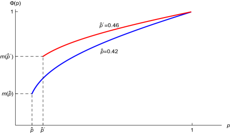
Figure 6: The invariant distribution of $p$ under alternative cutoffs

Suppose the PM lowers the threshold say from $\hat{p}^{\prime}$ to $\hat{p}<\hat{p}^{\prime}$. Then, the point mass at the threshold shrinks, i.e., $m(\hat{p})<m(\hat{p}^{\prime})$. In other words, the PM’s belief spends less time at its cutoff when the cutoff is lower. There are two reasons for this. Imagine that the beliefs under two cutoff policies are “coupled” at some level $p>\hat{p}^{\prime}$. Then, absent detection, the PM’s belief under both policies drifts down at the same rate until it reaches $\hat{p}^{\prime}$. When it does, the belief stops moving under the policy with cutoff $\hat{p}^{\prime}$, but it continues its downward march under the policy with cutoff $\hat{p}$. Only when it reaches $\hat{p}$, does the belief stop moving under the latter policy. Namely, it takes a longer time to reach the lower cutoff when the cutoff is lower. Second, once the belief has reached its cutoff, the learning is slowed since the PM lowers its enforcement to a level, but more so when the cutoff is higher, since $z(\hat{p})>z(\hat{p}^{\prime})$ when $\hat{p}<\hat{p}^{\prime}$. This means that the belief leaves, in fact, jumps out of, the cutoff at a faster rate when the cutoff is lower. This means that it takes less time for the belief to leave the cutoff when it is lower. Combining the two effects, the belief spends less time at the lower cutoff than at the higher cutoff, so $m(\hat{p})<m(\hat{p}^{\prime})$, as shown in Figure 6. The figure also shows the sense in which the belief distribution is more dispersed when the cutoff is lower, suggesting that more enforcement, implied by a lower cutoff, entails more “learning.”

Ultimately, what a potential criminal cares about is the expected enforcement

$$\mathbb{E}_{p}[y_{\hat{p}}(p)]=m(\hat{p})z(\hat{p})+(1-m(\hat{p}))\cdot 1.$$

Since $m(\hat{p})$ is increasing and $z(\hat{p})<1$ is decreasing in $\hat{p}$, the (conditional) expected enforcement faced by a potential criminal is decreasing in $\hat{p}$. This conforms to the intuition that a lower cutoff policy involves a higher expected enforcement level.

Lemma 2.

Given any cutoff policy $y_{\hat{p}}(\cdot)$ with $\hat{p}\in[\pi_{1},\pi_{0}]$,

• the point mass $m(\hat{p})$ is strictly decreasing in $\hat{p}$, and $m(\hat{p})\to 0$ as $\hat{p}\to\pi_{1}$ and $m(\hat{p})\to 1$ as $\hat{p}\to\pi_{0}$.

• the (conditional) expected enforcement $\mathbb{E}_{p}[y_{\hat{p}}(p)]$ is strictly decreasing in $\hat{p}$, and $\mathbb{E}_{p}[y_{\hat{p}}(p)]\to 1$ as $\hat{p}\to\pi_{1}$ and $\mathbb{E}_{p}[y_{\hat{p}}(p)]\to 0$ as $\hat{p}\to\pi_{0}$.

• therefore, there exists a unique $\hat{p}^{*}\in(\pi_{1},\pi_{0})$ such that $\mathbb{E}_{p}[y_{\hat{p}^{*}}(p)]=\hat{y}.$

Proof.

See Section C.1. ∎

The last observation (iii) will be particularly useful for our equilibrium analysis for GP and OP. It means that if the PM uses a policy with cutoff $\hat{p}^{*}$, then potential criminals will face the expected enforcement level of $\hat{y}$, so they will become indifferent to committing a crime.

4.3 Greedy predictive enforcement

We are now ready to study the PM’s behavior under GP. Suppose first $\pi_{0}\lambda<c$. Then, much like NP, eventually, no enforcement will be chosen since the benefit of enforcement is not worth the cost. Hence, the unique equilibrium is $(x_{\text{\tiny GP}},y_{\text{\tiny GP}})=(1,0).$

Suppose next $\pi_{0}\lambda\geq c$. One can easily see that there is no pure strategy equilibrium. Hence, consider a mixed strategy equilibrium in which a potential crime with a crime opportunity commits a crime with probability $x_{\text{\tiny GP}}\in(0,1)$.

Meanwhile, under GP, PM chooses an enforcement policy $y_{\text{\tiny GP}}(p)$ which equals $1$ if $p>\hat{p}_{M}$ and $z(\hat{p}_{M})$ if $p=\hat{p}_{M}$, where the myopic cutoff is $\hat{p}_{M}=c/(x_{\text{\tiny GP}}\lambda)$. For a criminal to randomize, his expected enforcement level must be $\hat{y}$. By 2-(iii), this requires that

$$\hat{p}_{M}=\hat{p}^{*},$$

or

$$x_{\text{\tiny GP}}=\frac{c}{\hat{p}^{*}\lambda}.$$ (10)

With this construction, the PM uses her greedy policy with cutoff $\hat{p}_{M}=\hat{p}^{*}$, which then yields the expected enforcement level of $\hat{y}$, so a potential criminal is indifferent and commits a crime with probability $x_{\text{\tiny GP}}$.

Proposition 5.

• If $\lambda<\frac{c}{\pi_{0}}$, then GP admits a unique equilibrium $(x_{\text{\tiny GP}},y_{\text{\tiny GP}})=(1,0)$;

• If $\lambda\geq\frac{c}{\pi_{0}}$, then GP admits a unique equilibrium in which $x_{GP}=\min\{\frac{c}{\hat{p}^{*}\lambda},1\}$, and $y_{\text{\tiny GP}}(p)=1$ for $p>\max\{\hat{p}^{*},\frac{c}{\lambda}\}$ and $y_{\text{\tiny GP}}(p)=z(p)$ for $p=\max\{\hat{p}^{*},\frac{c}{\lambda}\}$.

4.4 Optimal predictive enforcement

We now study the Markov perfect equilibrium under OP. Recall from 1 that the PM’s best response to a crime level $x$ depends on where the optimal cutoff $\hat{p}(\lambda x)$ lies in the relationship with thresholds, $\pi_{1}$ and $\pi_{0}$, where we make the dependence of $\hat{p}$ on $x\lambda$ explicit now that $x$ is endogenous.

Suppose first that $\lambda<{\Lambda}^{-}(c)$. Then, for any $x\in[0,1]$, we have $\hat{p}(\lambda x)>\pi_{0}$, which means that the enforcement only occurs at $p\geq\hat{p}(\lambda x)>\pi_{0}$. Thus, the long-run belief will be at $\pi_{0}$, so no enforcement will be chosen in the long run. Given this, each criminal’s best response is to choose $x=1$. Hence, the unique equilibrium is $(x_{OP},y_{OP})=(1,0).$

Suppose next that $\lambda\geq{\Lambda}^{-}(c)$. There are two cases to consider depending on whether $\lambda\geq\Lambda^{*}(c)$, where $\Lambda^{*}(c)$ is the crime rate that incentivizes the PM to choose the cutoff $\hat{p}^{*}$ under OP, or

$$\hat{p}(\Lambda^{*}(c))=\hat{p}^{*}.$$

Note that ${\Lambda}^{-}(c)<\Lambda^{*}(c)<{\Lambda}^{+}(c)$. If $\lambda\in({\Lambda}^{-}(c),\Lambda^{*}(c))$, then even with $x=1$, the cutoff for PM’s OP cutoff will be above $\hat{p}^{*}$, which implies that the enforcement level $\mathbb{E}_{p}[y_{\hat{p}(\lambda)}(p)]$ will fall short of $\hat{y}$. Thus, each criminal will choose $x=1$, to which PM best responds by adopting cutoff $\hat{p}(\lambda)$ as cutoff: that is, $y=1$ at $p>\hat{p}(\lambda)$ and $y=z(p)$ at $p=\hat{p}(\lambda)$.

If $\lambda\geq\Lambda^{*}(c)$, then criminals must randomize. This requires the OP cutoff $\hat{p}(\lambda x)$ to equal $\hat{p}^{*}$ so that the associated enforcement level equals $\hat{y}$. This in turn requires $\lambda x=\Lambda^{*}(c)$, which pins down $x=\Lambda^{*}(c)/\lambda$.

Given this policy, the equilibrium enforcement level is equal to $\hat{y}$, to which criminals best respond by randomization with probability $x=\Lambda^{*}(c)/\lambda$. Hence, we obtain the following result:

Proposition 6.

• If $\lambda<{\Lambda}^{-}(c)$, then OP admits a unique equilibrium $(x_{\text{\tiny OP}},y_{\text{\tiny OP}})=(1,0)$;

• If $\lambda\geq{\Lambda}^{-}(c)$, then OP admits a unique equilibrium in which $x_{\text{\tiny OP}}=\min\{\frac{\Lambda^{*}(c)}{\lambda},1\}$, and $y_{\text{\tiny OP}}(p)=1$ for $p>\max\{\hat{p}^{*},\hat{p}(\lambda)\}$ and $y_{\text{\tiny OP}}(p)=z(p)$ for $p=\max\{\hat{p}^{*},\hat{p}(\lambda)\}$.

Similar to NP and GP, if $\lambda$ is sufficiently low, then crime is unlikely even with $x=1$, so the PM chooses no enforcement in OP. If $\lambda$ is not so low, then the PM employs a cutoff $\hat{p}=\max\{\hat{p}^{*},\hat{p}(\lambda)\}$. If $\lambda$ is sufficiently large, then the cutoff equals $\hat{p}^{*}$. In particular, for $\lambda\geq c/\pi_{0}$, the PM would adopt the same enforcement in GP (see 5). Then, the enforcement level is the same between OP and GP! This may appear puzzling in light of 2, which suggests that, facing the same $x$, the PM chooses a strictly lower cutoff under OP than under GP, whenever her OP cutoff $\hat{p}$ lies in $(\pi_{1},\pi_{0})$. The answer to the puzzle is that criminals do not behave the same in both regimes. Indeed, for the PM to be willing to choose the same enforcement policy, it must be that she faces a lower crime rate under OP than under GP. This is precisely the case. As will be formally stated later, one can show that $x_{\text{\tiny OP}}<x_{\text{\tiny GP}}$, whenever $x_{\text{\tiny OP}}<1$. In other words, facing the PM with a stronger desire to enforce (due to her informational motive) under OP, a potential criminal adjusts his crime level below what he would choose under GP; in equilibrium he does so to a level that leads the PM to choose the same enforcement level in OP as in GP.

4.5 Comparing Regimes

We are now ready to compare the performances of alternative regimes. The endogenous crimes case bring a new important purpose of law enforcement: deterrence. The threat of enforcement can now discourage criminals from committing crimes. If the PM can commit to its enforcement level, then he could eliminate all crimes. Our PM does not have such a commitment power even in OP; she can only react optimally to the steady state equilibrium level of crime rate. Hence, unlike the exogenous crimes case, OP is no longer trivially superior to the other regimes with endogenous crimes. Nevertheless, as will be seen, the OP leads to more deterrence and lower expected losses, compared with NP and GP. The comparison follows:

Proposition 7.

With endogenous enforcement, the three regimes are compared as follows:

1. If $\lambda\leq{\Lambda}^{-}(c)$, then all three regimes lead to the identical equilibrium in which $x=1$ and the PM never enforces (i.e., $y=0$).

2. If ${\Lambda}^{-}(c)<\lambda\leq\frac{c}{\pi_{0}}$, then $x=1$ in all three regimes; the PM never enforces under NP and GP, but employs a cutoff policy cutoff $\hat{p}(\lambda)$ under OP.

3. If $\frac{c}{\pi_{0}}<\lambda\leq\Lambda^{*}(c)$, then $x_{\text{\tiny GP}}=x_{\text{\tiny OP}}=1>x_{\text{\tiny NP}}=\frac{c}{\pi_{0}\lambda}$; the PM enforces with $\hat{y}$ under NP, but employs cutoff policies with cutoffs $\hat{p}_{M}=\frac{c}{\lambda}$ and $\hat{p}(\lambda)<\frac{c}{\lambda}$ under GP and OP, respectively.

4. If $\Lambda^{*}(c)<\lambda<\frac{c}{\hat{p}^{*}}$, then $x_{\text{\tiny GP}}=1>x_{\text{\tiny OP}}=\frac{\Lambda^{*}(c)}{\lambda}>x_{\text{\tiny NP}}=\frac{c}{\pi_{0}\lambda}$, and the PM enforces with $\hat{y}$ under NP, but follows cutoff policies with cutoffs $\hat{p}_{M}=\frac{c}{\lambda}$ and $\hat{p}^{*}<\frac{c}{\lambda}$ under GP and OP, respectively.

5. If $\lambda\geq\frac{c}{\hat{p}^{*}}$, then $x_{\text{\tiny GP}}=\frac{c}{\hat{p}^{*}\lambda}>x_{\text{\tiny OP}}=\frac{\Lambda^{*}(c)}{\lambda}>x_{\text{\tiny NP}}=\frac{c}{\pi_{0}\lambda}$; $y_{\text{\tiny NP}}=\hat{y}$, and both $y_{\text{\tiny GP}}(\cdot)$ and $y_{\text{\tiny OP}}(\cdot)$ involves the identical cutoff $\hat{p}^{*}$.

In all cases, the total loss is the same between NP and GP. OP entails the same total loss in Case (i). In other cases, OP entails a strictly smaller loss.

Several remarks are in order. First, the alternative regimes entail differing levels of enforcement. When $\lambda$ is large enough to be in cases (iii)-(v), the PM enforces most under NP, followed by OP, and then GP. Firstly, it takes a larger value of $\lambda$ for the PM to be willing to enforce under OP than under NP, and under GP than under OP. Second, conditional on enforcing, the PM also uses less resources due to the targeted nature of predictive enforcement. When the PM enforces under NP, she chooses the “marginally deterring” level of enforcement $\hat{y}$ regardless of the state. For $\lambda$ high enough, the PM again chooses a marginally deterring level $\hat{y}$ but conditional on $\omega=H$. She enforces strictly less in state $\omega=L$. In other words, prediction allows the PM to be more targeted in her allocation of enforcement resources toward state $\omega=H$.

Second, the equilibrium deterrence levels also differ across the regimes. The deterrence is highest under NP, followed by OP, and the lowest under GP. This is explained by the PM’s incentive for enforcement. Under either GP or OP, the PM must have incentives for enforcement at the respective cutoff beliefs, $\hat{p}$, which by the martingale property are lower than $\pi_{0}$, the belief at which the PM must be incentivized to enforce. Hence, it takes higher crime rates to motivate the PM to enforce under either GP or OP than under NP. Next, between GP and OP, facing the same crime rate, the PM has stronger incentives to enforce under OP than under GP. Hence, it takes a lower crime rate to incentivize the PM to enforce under OP than under GP.

Most important is the welfare comparison. Firstly, the equivalence between NP and GP carries over to the endogenous crime case. This is obvious in cases (i) and (ii). In cases (iii)-(v), NP and GP differ both in enforcement and deterrence levels: the PM enforces and deters more in NP than in GP, where enforcement is more targeted toward the criminal state $\omega=H$. Despite the differences, the two policies entail the same loss the same because, when the GP calls for reduced enforcement, the belief is at $\hat{p}_{M}=c/(x_{\text{\tiny GP}}\lambda)$, so the enforcement is payoff-irrelevant: the total loss is the same as if the PM always enforces.

Finally, OP entails strictly lower expected loss than the other regime for all cases except (i), where all three regimes are equivalent. In cases (ii) and (iii), the PM faces the same crime rate but acts optimally under OP but not under GP, according to 3. In cases (iv) and (v(, the OP picks an optimal enforcement level against a crime rate strictly lower than is induced by GP. Since GP’s choice of the enforcement level is not optimal against the crime rate, OP performs strictly better GP.

The intuition behind the superior performance for OP except for Case (i) can be traced to what we may regard as an unintended benefit of informational sophistication on the part of PM. The informational acquisition motive leads the PM to explore more under OP than under GP, which results in the PM enforcing more aggressively. Essentially, 7 suggests that this has the added benefit of helping PM to credibly commit to deter crime.

4.6 Predictive crime

So far, we have assumed that the PM can enforce predictively in a way criminals cannot in their crime decisions. This assumption is realistic in many regulatory contexts where enforcement agencies collect crime data privately and have an option not to publicly disclose that data. But in some other context, for instance, in the case of common crimes (e.g., street robbery, and drug-related offenses), the crime data may be widely available and may be updated reasonably frequently, and news media could also make the information more widely available. Even in other cases, potential offenders may become as savvy as enforcement agencies in making use of data.

In this subsection, we assume that the crime decision is as informed by the past crime data as the PM’s enforcement decision. Independently of the plausibility of this scenario, considering it will help us understand to role of informational advantage PM has over potential criminals.

In the case of NP, since PM has no information other than $\pi_{0}$, criminals access no more information, so the analysis remains unchanged.

In the case of GP and OP, the results do change except for case (i) of 7. Assume $\lambda>{\Lambda}^{-}(c)$, and let $(y(p),x(p))$ denote the enforcement and crime levels in equilibrium for any posterior $p$ in the support. In both regimes, it is a Markov perfect equilibrium for the PM to enforce at $y(p)=\hat{y}$ if and only if $p\geq\hat{p}=\frac{c}{\lambda}$. In response, potential criminals choose

$$x(p)=\frac{c}{p\lambda},$$

which keeps the PM indifferent, for each $p\geq\hat{p}$. Essentially, criminals and the PM play the “inspection game” equilibrium for each $p\geq\hat{p}$. Consequently, the expected total loss is the same across all three regimes.

Proposition 8.

If potential criminals base their decision on the posterior that PM accesses, all three regimes result in the same total expected loss.

Proof.

See Appendix D. ∎

This result, together with 7, suggests that the PM’s informational advantage is important for her to realize the value of predictive enforcement.

5 Conclusion

We have developed a model of predictive enforcement that accounts for the feedback between enforcement and data collection. The analysis demonstrates the potential for the prediction to improve enforcement decisions and deter crimes. At the same time, it highlights the importance of how prediction should guide enforcement. Using prediction to achieve the current enforcement objective without accounting for the future informational implications performs poorly. It can perform as poorly as if no prediction and data were used, when prediction can be achieved only as a result of active surveillance/enforcement, as in the case of victimless crimes. Further, such a myopic use of data can lead to over-enforcement of the traditionally high-crime neighborhood. Our analysis is thus consistent with the prevailing criticism about the discriminatory nature of predictive policing and provides a theoretical mechanism for it. We also find that the information acquisition motive by the enforcement authority can enhance the credibility of enforcement and increase deterrence.

Appendix A Proof of 1

Let us first derive an ODE for the total (expected) discounted amount of both deterred and undeterred crimes, denoted $C(p)$, when the probability of $\omega=I$ at $t$ is $p$. Since whether a crime occurs is independent of the PM’s policy, we have for any $y\in[0,1]$,

$$C(p)= p\lambda xdt+p\lambda xydt(1-rdt)C(1)+(1-rdt)(1-p\lambda xydt)C(p_{t+dt})$$

$$= p\lambda xdt+p\lambda xydt(1-rdt)C(1)+(1-rdt)(1-p\lambda xydt)\left(C(p)+f(p,y)C^{\prime}(p)dt\right)$$

$$\implies rC(p)= p\lambda x+p\lambda xy\left(C(1)-C(p)\right)+f(p,y)C^{\prime}(p).$$

Thus,

$$p\lambda xy\left(C(1)-C(p)\right)+f(p,y)C^{\prime}(p)=f(p,0)C^{\prime}(p)$$ (11)

Given any policy $y:[0,1]\to[0,1]$, let us define $V_{y}$ analogously to $L_{y}$: that is, $V_{y}$ is the total discounted value of deterred crimes minus enforcement costs associated with $y$. Note that for any policy $y$, we have $V_{y}(p)+L_{y}(p)=C(p)$ at each $p\in[0,1]$ since the terms of enforcement cost in $V_{y}$ and $L_{y}$ cancel out so $V_{y}(\cdot)$ and $L_{y}(\cdot)$ sum to the total discounted amount of deterred and undeterred crimes.

Let $y^{*}$ be the optimal policy that solves 6. Fix any $p\in[0,1]$ and let $z^{*}=y^{*}(p)$. Then, we obtain for any policy $y:[0,1]\to[0,1]$

$$rL_{y^{*}}(p) =p\lambda x(1-z^{*})+cz^{*}+p\lambda xz^{*}\left[L_{y^{*}}(1)-L_{y^{*}}(p)\right]+f(p,z^{*})L_{y^{*}}^{\prime}(p)$$

$$=p\lambda x(1-z^{*})+cz^{*}+p\lambda xz^{*}\left[C(1)-V_{y^{*}}(1)-(C(p)-V_{y^{*}}(p))\right]+f(p,z^{*})(C^{\prime}(p)-V_{y^{*}}^{\prime}(p))$$

$$=p\lambda x+f(p,0)C^{\prime}(p)-\Big{[}p\lambda xz^{*}-cz^{*}+p\lambda xz^{*}(V_{y^{*}}(1)-V_{y^{*}}(p))+f(p,z^{*})V_{y^{*}}^{\prime}(p)\Big{]}$$

$$\leq p\lambda x+f(p,0)C^{\prime}(p)-\Big{[}p\lambda xy(p)-cy(p)+p\lambda xy(p)(V_{y}(1)-V_{y}(p))+f(p,y(p))V_{y}^{\prime}(p)\Big{]}$$

$$=rL_{y}(p),$$

where the third equality follows from 11 while the inequality from the optimality of $y^{*}$. The last equality holds for the same reason that the first three equalities hold. Hence, $y^{*}$ solves 5.

The proof that any optimal policy $y^{*}$ solves (5) solves (6) as well is analogous and hence omitted.

Appendix B Proof of 1

B.1 Preliminary Results for the Analysis of HJB Equation

This section provides the analysis of HJB equation (6), leading to the proof of 1. Throughout our analysis in this section, we use $\tau$ to denote a vector of parameters $(\lambda,x,c)$.

As noted earlier, an important element in our model is the evolution of PM’s belief given by $f(p,y)$. We let $g(p):=f(p,1)$ and $h(p):=f(p,0)$, that is,

$$g(p) =\rho_{L}(1-p)-\rho_{H}p-p(1-p){\lambda}x$$

$$h(p) =\rho_{L}(1-p)-\rho_{H}p.$$

Observe that $h(\pi_{0})=0$ and that $h(p)$ is strictly decreasing so $h(p)>(<)0$ for $p<(>)\pi_{0}$. Meanwhile, $\pi_{1}$ is a unique root of $g(p)$ in the interval $[0,1]$. Also, $g$ is single crossing, namely, $g(p)>(<)0$ for $p<(>)\pi_{1}$. It is straightforward to prove the following result:

Lemma 3.

$\pi_{1}<\pi_{0}$ while $\pi_{1}$ decreases from $\pi_{0}$ to 0 as $\lambda x$ increases from 0 to $\infty$.

Given the cutoff policy and the definitions of $g(p)$ and $h(p)$, (6) becomes

$$rV(p)=h(p)V^{\prime}(p)\mbox{ for }p<\hat{p}$$ (12)

while it becomes

$$rV(p)=p\lambda x-c+p\lambda x\left[V(1)-V(p)\right]+g(p)V^{\prime}(p)\mbox{ for }p\geq\hat{p}.$$ (13)

To tackle the problem of endogenous boundary value $V(1)$, we parametrize the ODE in (13) as follows: $V(1)=K$ and

$$rV(p)=p\lambda x-c+p\lambda x\left[K-V(p)\right]+g(p)V^{\prime}(p).$$ (14)

Letting $D[K]$ denote the parametrized ODE, the following result provides a set of properties for the solution to $D[K]$, which will prove useful throughout our analysis.

Lemma 4.

For any given $\varepsilon>0$,

• $D[K]$ has a unique solution over $[\pi_{1}+\varepsilon,1]$, denoted $V[p;K]$. Also, $V[p;K]$ and $V^{\prime}[p;K]$ are continuous in $\lambda$, $x$, and $c$ as well as $p$ and $K$;

• With $K=\underline{K}(\tau):=\frac{(\lambda x-c)(r+\rho_{L})-c\rho_{H}}{r(r+\rho_{L}+\rho_{H})}$, $V[p;K]$ is linear with the slope equal to $\frac{\lambda x}{r+\rho_{L}+\rho_{H}}$;

• $V^{\prime}(p;K)$ is strictly decreasing in $K$ while $V(p;K)$ is strictly increasing in $K$;

• For $p>\pi_{1}$, $V^{\prime\prime}(p;K)$ is strictly increasing in $K$ while $V^{\prime\prime}(p;K)\gtreqqless 0$ if $K\gtreqqless\underline{K}(\tau)$;

• As $K\to\infty$, $V^{\prime\prime}(p;K)\to\infty$ for all $p>\pi_{1}$ while $V^{\prime}(p;K)<0$ for all $p>\pi_{1}$ if $K$ is sufficiently large.

Proof.

Part (i) follows from the standard result in differential equations, provided that the coefficient for $V^{\prime}$ (i.e., $g(p)$) is bounded away from zero over $[\pi_{1}+\varepsilon,1]$ (recall that $g(p)<0$ for any $p>\pi_{1}$).

Part (ii) is established by finding a linear solution for $D[K]$ constructively. To do so, let $V(p)=K+a(p-1)$ for $p\in[\hat{p},1]$. Then, the RHS of (14) becomes

$$p\lambda x-c+p\lambda xa(1-p)+[\rho_{L}(1-p)-\rho_{H}p-p(1-p){\lambda}x]a$$

$$= -c+\rho_{L}a+[\lambda x-(\rho_{L}+\rho_{H})a]p,$$

which must equal the LHS of (14), $rV(p)=r(K+a(p-1))=r(K-a)+rap.$ We must thus have $\rho_{L}a=r(K-a)$ and $\lambda x-(\rho_{L}+\rho_{H})a=ra$, which can be solved to yield $a=\frac{\lambda x}{r+\rho_{L}+\rho_{H}}$ and $K=\frac{(\lambda x-c)(r+\rho_{L})-c\rho_{H}}{r(r+\rho_{L}+\rho_{H})}$, as desired.

To prove Part (iii), let us consider any $K_{2}>K_{1}$. For simplicity, let $V_{i}(\cdot)$ denote $V(\cdot;K_{i})$ for $i=1,2$. To begin, let us substitute $p=1$ and $V_{i}(1)=K_{i}$ into (14) to obtain

$$rK_{i}=\lambda x-c-\rho_{H}V_{i}^{\prime}(1)\;\mbox{ or }\;V_{i}^{\prime}(1)=\frac{\lambda x-c-rK_{i}}{\rho_{H}},$$ (15)

implying $V_{1}^{\prime}(1)>V_{2}^{\prime}(1)$. Suppose now for contradiction that there is some $p<1$ such that $V_{1}^{\prime}(p)\leq V_{2}^{\prime}(p)$. One can then find some $p^{\prime}<1$ such that $V_{1}^{\prime}(p^{\prime})=V_{2}^{\prime}(p^{\prime})$ and $V_{1}^{\prime}(p)>V_{2}^{\prime}(p),\forall p>p^{\prime}$. Note first that

$$V_{1}(p^{\prime})=V_{1}(1)-\int_{p^{\prime}}^{1}V_{1}^{\prime}(p)dp<V_{2}(1)-\int_{p^{\prime}}^{1}V_{2}^{\prime}(p)dp=V_{2}(p^{\prime})$$ (16)

since $V_{1}(1)=K_{1}<K_{2}=V_{2}(1)$ and $V_{1}^{\prime}(p)<V_{2}^{\prime}(p),\forall p\in[p^{\prime},1]$. We then rewrite (14) with $p=p^{\prime}$, $V=V_{i}$, and $K=V_{i}(1)$ as

$$g(p^{\prime})V_{i}^{\prime}(p^{\prime})+p^{\prime}\lambda x-c=rV_{i}(p^{\prime})-p^{\prime}\lambda x[V_{i}(1)-V_{i}(p^{\prime})].$$

With $V_{1}^{\prime}(p^{\prime})=V_{2}^{\prime}(p^{\prime})$, the LHS of this equation remains unchanged across $i=1,2$, so must be the RHS. However,

$$rV_{1}(p^{\prime})-p^{\prime}\lambda x[V_{1}(1)-V_{1}(p^{\prime})] =rV_{1}(p^{\prime})-p^{\prime}\lambda x\int_{p^{\prime}}^{1}V_{1}^{\prime}(p)dp$$

$$<rV_{2}(p^{\prime})-p^{\prime}\lambda x\int_{p^{\prime}}^{1}V_{2}^{\prime}(p)dp$$

$$=rV_{2}(p^{\prime})-p^{\prime}\lambda x[V_{2}(1)-V_{2}(p^{\prime})],$$

where the inequality holds since $V_{2}(p^{\prime})>V_{1}(p^{\prime})$ from (16) and $V_{2}^{\prime}(p)<V_{1}^{\prime}(p),\forall p>p^{\prime}$. We have thus obtained a contradiction. That $V(p;K)$ is strictly increasing in $K$ can be established by an analogous argument, so its proof is omitted.

For Part (iv), let us differentiate both sides of (14) to obtain

$$rV^{\prime}(p;K)=\lambda x(1+K)-\lambda xV(p;K)+\left(g^{\prime}(p)-p\lambda x\right)V^{\prime}(p;K)+g(p)V^{\prime\prime}(p;K),$$

which can be combined with (14) to remove $V(p)$ and obtain

$$V^{\prime\prime}(p;K)=\frac{\left[r^{2}+r(\lambda x+\rho_{H}+\rho_{L})+\lambda x\rho_{L}\right]V^{\prime}(p;K)-\lambda x(c+r+rK)}{(r+\lambda px)g(p)}.$$ (17)

Since the numerator is strictly decreasing in $K$ and the denominator is negative (recall $g(p)<0$ for $p>\pi_{1}$), $V^{\prime\prime}(p;K)$ is strictly increasing in $K$. Combining this with Part (ii) proves the rest of Part (iv).

To prove Part (v), observe first that the numerator in (17) goes to $-\infty$ for all $p>\pi_{1}$ as $K\to\infty$ while the denominator is negative and bounded (from below), from which the first result follows. Also, by (15) and Part (iv), $V^{\prime}(1;K)<0$ and $V^{\prime\prime}(p;K)>0$ for sufficiently large $K$, which implies $V^{\prime}(p;K)<0$ for $p\in(\pi_{1},1)$, proving the second result. ∎

B.2 Necessary Conditions for the Solution of HJB Equation

This section provides a set of conditions that must be satisfied by any solution of HJB equation.

First of all, we require the value matching and smooth pasting: that is, $V(\hat{p}_{-})=V(\hat{p}_{+})$ and $V^{\prime}(\hat{p}_{-})=V^{\prime}(\hat{p}_{+})$, respectively. The these conditions are related to the function $\Delta$ as follows:

Lemma 5.

• If the value matching holds, then the smooth pasting is equivalent to $\Delta(\hat{p}_{+})=0$ unless $\hat{p}=\pi_{0}$;

• If the smooth pasting holds, then the value matching is equivalent to $\Delta(\hat{p}_{+})=0$.

Proof.

Note first that using $g(p)=h(p)-\lambda px(1-p)$, we can rewrite (13) as

$$rV(p)=h(p)V^{\prime}(p)+x\Delta(p)\mbox{ for }p\geq\hat{p}.$$ (18)

To prove Part (i), suppose that the value matching holds. Then, by (12) and (18),

$$h(\hat{p})V^{\prime}(\hat{p}_{+})+x\Delta(\hat{p}_{+})=rV(\hat{p}_{+})=rV(\hat{p}_{-})=h(\hat{p})V^{\prime}(\hat{p}_{-})$$

or

$$h(\hat{p})V^{\prime}(\hat{p}_{+})+x\Delta(\hat{p}_{+})=h(\hat{p})V^{\prime}(\hat{p}_{-}).$$

Thus, $\Delta(\hat{p}_{+})=0$ is equivalent to $V^{\prime}(\hat{p}_{+})=V^{\prime}(\hat{p}_{-})$ unless $\hat{p}=\pi_{0}$. The proof of Part (ii) is analogous and hence omitted. ∎

The optimality of cutoff policy $y(p)=1_{\{p\geq\hat{p}\}}$ also requires that $\frac{\partial W(p,y)}{\partial y}$ be ‘single-crossing’ at $p=\hat{p}$: that is, $\frac{\partial W(p,y)}{\partial y}\leq(\geq)0$ if $p\leq(\geq)\hat{p}$. Given that $\Delta(p)=\frac{1}{x}\frac{\partial W(p,y)}{\partial y}=0$ at $p=\hat{p}$ (as shown in 5), this requires $\Delta^{\prime}(\hat{p}_{-})\geq 0$ and $\Delta^{\prime}(\hat{p}_{+})\geq 0$. The next result shows an additional condition this constraint imposes on the value function $V$:

Lemma 6.

Letting

$$\sigma(p):=\frac{h(p)c}{p^{2}(1-p)\lambda x(r+\rho_{L}+\rho_{H})},$$

we must have

$$\Delta^{\prime}(\hat{p}_{-})=\frac{\hat{p}(1-\hat{p})\lambda(r+\rho_{L}+\rho_{H})}{h(\hat{p})}\left[\sigma(\hat{p})-V^{\prime}(\hat{p})\right]\geq 0\mbox{ for }\hat{p}\neq\pi_{0}$$ (19)

and

$$\Delta^{\prime}(\hat{p}_{+})=\frac{\hat{p}(1-\hat{p})\lambda(r+\rho_{L}+\rho_{H})}{g(\hat{p})}\left[\sigma(\hat{p})-V^{\prime}(\hat{p})\right]\geq 0\mbox{ for }\hat{p}\neq\pi_{1}.$$ (20)

Proof.

Let us first differentiate both sides of (12) to get $rV^{\prime}(p)=h^{\prime}(p)V^{\prime}(p)+h(p)V^{\prime\prime}(p)$, which can be simplified to

$$h(p)V^{\prime\prime}(p) =(r+\rho_{L}+\rho_{H})V^{\prime}(p).$$

Substituting this into the differentiation of $\Delta(p)$, we obtain for $p\leq\hat{p}$ with $p\neq\pi_{0}$,

$$\Delta^{\prime}(p) =\frac{\Delta(p)}{p}+\frac{c}{px}-p(1-p)\lambda V^{\prime\prime}(p)$$

$$=\frac{\Delta(p)}{p}+\frac{c}{px}-\frac{p(1-p)\lambda(r+\rho_{L}+\rho_{H})}{h(p)}V^{\prime}(p),$$

$$=\frac{\Delta(p)}{p}+\frac{p(1-p)\lambda(r+\rho_{L}+\rho_{H})}{h(p)}\left[\sigma(p)-V^{\prime}(p)\right]$$ (21)

where the first equality follows straightforwardly from the definition of $\Delta(\cdot)$. Then, (19) follows from observing that $\Delta(\hat{p}_{-})=0$

Let us next differentiate both sides of (13) to get

$$rV^{\prime}(p)=\lambda x+\lambda x[V(1)-V(p)]-p\lambda xV^{\prime}(p)+g^{\prime}(p)V^{\prime}(p)+g(p)V^{\prime\prime}(p),$$

where $g(p)=\rho_{L}(1-p)-\rho_{H}p-p(1-p){\lambda}x$. Simplifying:

$$g(p)V^{\prime\prime}(p) =(r-g^{\prime}(p)+p\lambda x)V^{\prime}(p)+\lambda x[V(p)-(1+V(1))]$$

$$=(r+\rho_{L}+\rho_{H})V^{\prime}(p)+(1-p)\lambda xV^{\prime}(p)+\lambda x[V(p)-(1+V(1))]$$

$$=(r+\rho_{L}+\rho_{H})V^{\prime}(p)-\frac{c}{p}-\frac{\Delta(p)x}{p}.$$ (22)

Substituting this into the differentiation of $\Delta(p)$, we obtain for $p\geq\hat{p}$ with $p\neq\pi_{1}$,

$$\Delta^{\prime}(p) =\frac{\Delta(p)}{p}+\frac{c}{px}-p(1-p)\lambda V^{\prime\prime}(p)$$

$$=\frac{\Delta(p)}{p}+\frac{c}{px}-p(1-p)\lambda\frac{(r+\rho_{L}+\rho_{H})V^{\prime}(p)-\frac{c}{p}-\frac{\Delta(p)x}{p}}{g(p)}$$

$$=\left(1+\frac{p(1-p)\lambda x}{g(p)}\right)\left(\frac{\Delta(p)}{p}+\frac{c}{px}\right)-\frac{p(1-p)\lambda(r+\rho_{L}+\rho_{H})}{g(p)}V^{\prime}(p)$$

$$=\left(\frac{h(p)}{g(p)}\right)\left(\frac{\Delta(p)}{p}+\frac{c}{px}\right)-\frac{p(1-p)\lambda(r+\rho_{L}+\rho_{H})}{g(p)}V^{\prime}(p)$$

$$=\left(\frac{h(p)}{g(p)}\right)\left(\frac{\Delta(p)}{p}\right)+\frac{p(1-p)\lambda(r+\rho_{L}+\rho_{H})}{g(p)}\left[\sigma(p)-V^{\prime}(p)\right],$$ (23)

from which (20) follows since $\Delta(\hat{p}_{+})=0$. ∎

As it turns out, the constraints in (20) and (19) are binding in the case $\hat{p}\in(\pi_{1},\pi_{0})$ (that is, Case 3). To see it, observe that if $\hat{p}\in(\pi_{1},\pi_{0})$, then we have $g(\hat{p})<0<h(\hat{p})$. Thus, the inequalities in (19) and (20) can hold simultaneously only if the expression within the square bracket is equal to zero, i.e., $V^{\prime}(\hat{p})=\sigma(\hat{p})$. We thus obtain:

Lemma 7.

If $\hat{p}\in(\pi_{1},\pi_{0})$, then

$$V^{\prime}(\hat{p})=\sigma(\hat{p})=\frac{h(\hat{p})c}{\hat{p}^{2}(1-\hat{p})\lambda x(r+\rho_{L}+\rho_{H})}$$ (24)

or equivalently $\Delta^{\prime}(\hat{p})=0$.

Letting

$${\Lambda}^{+}(c):=\begin{cases}\frac{c(\rho_{L}+\rho_{H}-c)}{(\rho_{L}-c)}&\mbox{if }\rho_{L}-c>0\\ \infty&\mbox{otherwise},\end{cases}$$ (25)

we establish results that are useful for our subsequent analysis:

Lemma 8.

• There exists a unique $\underline{p}<\pi_{0}$ such that

  $$\sigma(\underline{p})=\frac{\lambda x}{r+\rho_{L}+\rho_{H}}.$$ (26)

• The following inequalities are equivalent: (a) $\lambda x\geq{\Lambda}^{+}(c)$; (b) $\pi_{1}\geq\hat{p}_{M}$; (c) $\pi_{1}\geq\underline{p}$; (d) $\underline{p}\geq\hat{p}_{M}$.

Proof.

Part (i) follows from the continuity of $\sigma$ and this claim:

Claim 1.

$\sigma(p)$ strictly decreases from $\infty$ to $0$ as $p$ increases from 0 to $\pi_{0}$.

Proof.

Note first that $\frac{h(p)}{p^{2}(1-p)}$ is strictly decreasing on $[0,\pi_{0}]$:

$$\frac{d}{dp}\left(\frac{h(p)}{p^{2}(1-p)}\right) =\frac{-2p^{2}(\rho_{H}+\rho_{L})+p(\rho_{H}+4\rho_{L})-2\rho_{L}}{(1-p)^{2}p^{3}}$$

$$=\frac{-2(\rho_{H}+\rho_{L})(p-\pi_{0})^{2}+\frac{2(\rho_{L})^{2}}{\rho_{H}+\rho_{L}}+p\rho_{H}-2\rho_{L}}{(1-p)^{2}p^{3}}<0,$$

since the numerator is maximized at $p=\pi_{0}$ within the range $[0,\pi_{0}]$ and the maximized value is equal to $\frac{-\rho_{L}\rho_{H}}{\rho_{H}+\rho_{L}}<0$. Thus, $\sigma(p)$ is strictly decreasing. Then, the result follows from observing that $\sigma(0)=\infty$ and $\sigma(\pi_{0})=0$ since $h(0)>0=h(\pi_{0}).$∎

For Part (ii), let us first prove the following claim:

Claim 2.

$\lambda x\geq{\Lambda}^{+}(c)$ is equivalent to

$$\lambda x(\rho_{L}-c)+c(c-\rho_{L}-\rho_{H})\geq 0.$$ (27)

Proof.

Notice that if $\rho_{L}-c>0$, then 27 is just a rearrangement of $\lambda x\geq{\Lambda}^{+}(c)$. It thus suffices to show that 27 implies $\rho_{L}>c$. Otherwise, we would have

$$\mbox{LHS of \eqref{equiv1}}\leq c(\rho_{L}-c)+c(c-\rho_{L}-\rho_{H})=-c\rho_{H}<0,$$

where the first inequality holds since $\lambda x>c$.∎

To prove the equivalence between (a) and (b), observe first that solving $g(p)=0$ yields $\pi_{1}=\frac{\lambda x+\rho_{L}+\rho_{H}-\sqrt{(\lambda x+\rho_{L}+\rho_{H})^{2}-4\lambda x\rho_{L}}}{2\lambda x}.$ Thus,

$$\frac{c}{\lambda x}\leq\pi_{1} \Leftrightarrow\lambda+\rho_{L}+\rho_{H}-2c\geq\sqrt{(\lambda x+\rho_{L}+\rho_{H})^{2}-4\lambda x\rho_{L}}.$$ (28)

$$\Leftrightarrow\left(\lambda+\rho_{L}+\rho_{H}-2c\right)^{2}\geq(\lambda x+\rho_{L}+\rho_{H})^{2}-4\lambda x\rho_{L}.$$

$$\Leftrightarrow\lambda x(\rho_{L}-c)+c(c-\rho_{L}-\rho_{H})\geq 0,$$ (29)

if the LHS of (28) is nonnegative. Given this and 2, the equivalence between $\pi_{1}\geq\frac{c}{\lambda x}$ and $\lambda x\geq{\Lambda}^{+}(c)$ will follow if (27) implies that the LHS of (28) is nonnegative. To see this, recall that (27) implies $\rho_{L}>c$, so $\lambda+\rho_{L}+\rho_{H}-2c>\lambda+\rho_{H}-c>0$ since $\lambda\geq\lambda x>c$.

To prove the equivalence between (b) and (c), observe that since $0=g(\pi_{1})=h(\pi_{1})-\pi_{1}(1-\pi_{1})\lambda x$, we have

$$\sigma(\underline{p})-\sigma(\pi_{1})=\frac{\lambda x}{r+\rho_{L}+\rho_{H}}-\sigma(\pi_{1}) =\frac{\lambda x}{r+\rho_{L}+\rho_{H}}-\frac{h(\pi_{1})c}{\pi_{1}^{2}(1-\pi_{1})\lambda x(r+\rho_{L}+\rho_{H})}$$

$$=\frac{c}{r+\rho_{L}+\rho_{H}}\left(\frac{\lambda x}{c}-\frac{1}{\pi_{1}}\right)\geq 0.$$ (30)

Since $\sigma$ is decreasing, we have $\pi_{1}\geq\underline{p}$ if and only if $\pi_{1}\geq\hat{p}_{M}$.

For the equivalence between (d) and (a), observe

$$\sigma(\hat{p}_{M})-\sigma(\underline{p})=\frac{\lambda x(\rho_{L}-c)+c(c-\rho_{L}-\rho_{H})}{c(\lambda x-c)\left(\rho_{H}+\rho_{L}+r\right)}.$$

Thus, given that $\sigma$ is decreasing, $\underline{p}\geq\hat{p}_{M}$ is equivalent to $\lambda x(\rho_{L}-c)+c(c-\rho_{L}-\rho_{H})\geq 0$, which is equivalent to (a) due to 2. ∎

We are now ready to provide some conditions for Case 1 and Case 2 in which the solution of HJB equation must take a simple linear form on either $[0,\hat{p}]$ or $[\hat{p},1]$ with corresponding boundary values:

Lemma 9.

• $V(p)=0$ for all $p\in[0,\hat{p}]$ if and only if $\hat{p}\geq\pi_{0}$;

• $V(p)$ is linear on $[\hat{p},1]$ if and only if $\hat{p}\leq\pi_{1}$;

• If $V(p)$ is linear on $[\hat{p},1]$, then $\hat{p}=\hat{p}_{M}$, $V(1)=\frac{(\lambda x-c)(r+\rho_{L})-c\rho_{H}}{r(r+\rho_{L}+\rho_{H})}$, and $V^{\prime}(p)=\frac{\lambda x}{r+\rho_{L}+\rho_{H}}>0,\forall p\in[\hat{p},1]$.

Proof.

To prove the if direction of Part (i), observe first that with $\hat{p}\geq\pi_{0}$, (12) and $h(\pi_{0})=0$ together imply $V(\pi_{0})=0$. Suppose for contradiction that there is some $p<\pi_{0}$ such that $V(p)<0$. Then, we must have some $\check{p}\in(p,\pi_{0})$ such that $V(\check{p})<0$ and $V^{\prime}(\check{p})>0$. Since $h(\check{p})>0$ and thus $h(\check{p})V^{\prime}(\check{p})>0$, (12) implies $V(\check{p})>0$, a contradiction. Suppose next that there is $p<\pi_{0}$ such that $V(p)>0$. Then, we must have some $\check{p}\in(p,\pi_{0})$ such that $V(\check{p})>0$ and $V^{\prime}(\check{p})<0$. Since $h(\check{p})>0$ and thus $h(\check{p})V^{\prime}(\check{p})<0$, (12) implies $V(\check{p})<0$, a contradiction. The argument so far establishes $V(p)=0$ for all $p\leq\pi_{0}$. An analogous argument can be used to establish the same result for the range $[\pi_{0},\hat{p}]$.

To prove the only if direction of Part (i), suppose that $V(p)=0$ for all $p\in[0,\hat{p}]$. Then, $V^{\prime}(\hat{p}_{+})=V^{\prime}(\hat{p}_{-})=0$, which by (20) requires that $\frac{h(\hat{p})}{g(\hat{p})}\geq 0$. This cannot hold if $\hat{p}\in(\pi_{1},\pi_{0})$ since then $h(\hat{p})>0>g(\hat{p})$. If $\hat{p}\leq\pi_{1}$, then Lemma 10 implies $V^{\prime}(p_{+})>0$, a contradiction. The remaining possibility is $\hat{p}\geq\pi_{0}$, as desired.

Let us first prove Part (iii) before proving Part (ii). The argument for determining $V(1)$ and $V^{\prime}(p)$ is analogous to that in the proof of 4-(ii) and hence omitted. To show $\hat{p}=\frac{c}{\lambda x}$, observe that the linearity of $V$ over $[\hat{p},1]$ implies $V(1)-V(p)-V^{\prime}(p)(1-p)=0$ for all $p\geq\hat{p}$, which means

$$\Delta(p)=p\lambda-\frac{c}{x}.$$ (31)

Thus, $\Delta(\hat{p})=0$ requires $\hat{p}=\frac{c}{\lambda x}=\hat{p}_{M}$.

To prove the if direction of Part (ii), let us differentiate both sides of (13) to obtain

$$rV^{\prime}(p)=g^{\prime}(p)V^{\prime}(p)+g(p)V^{\prime\prime}(p)-\lambda xV(p)-p\lambda xV^{\prime}(p)+\lambda x(1+V(1)).$$

We can combine this equation and (13) to remove $V(p)$ and obtain

$$V^{\prime}(p)= \frac{\lambda x(c+r+rV(1))+(r+p\lambda x)g(p)V^{\prime\prime}(p)}{r^{2}+r(\lambda x+\rho_{L}+\rho_{H})+\lambda x\rho_{L}}.$$ (32)

Let us denote $a=\frac{\lambda x(c+r+rV(1))}{r^{2}+r(\lambda x+\rho_{L}+\rho_{H})+\lambda x\rho_{L}}$. We show that $V^{\prime}(p)=a,\forall p\geq\hat{p}.$ Note first that this is true for $p=\pi_{1}$ since $g(\pi_{1})=0$ and (32) imply $V^{\prime}(\pi_{1})=a$. To first prove the linearity of $V$ over $(\pi_{1},1]$, suppose not, i.e., $V^{\prime}(p)\neq a$ for some $p\in(\pi_{1},1]$. Consider first the case $V^{\prime}(p)>a$. We must then have some $\check{p}\in(\pi_{1},p)$ such that $V^{\prime\prime}(\check{p})>0$ and $V^{\prime}(\check{p})>a$. Since $g(\check{p})<0$ and thus $g(\check{p})V^{\prime\prime}(\check{p})<0$, the equation (32) implies $V^{\prime}(\check{p})<\frac{\lambda x(c+r+rV(1))}{r^{2}+r(\lambda x+\rho_{L}+\rho_{H})+\lambda x\rho_{L}}=a$, a contradiction. Consider next the case $V^{\prime}(p)<a$. Then, we must have some $\check{p}\in(\pi_{1},p)$ such that $V^{\prime\prime}(\check{p})<0$ and $V^{\prime}(\check{p})<a$. Since $g(\check{p})<0$ and thus $g(\check{p})V^{\prime\prime}(\check{p})>0$, the equation (32) implies $V^{\prime}(\check{p})>\frac{\lambda x(c+r+rV(1))}{r^{2}+r(\lambda x+\rho_{L}+\rho_{H})+\lambda x\rho_{L}}=a$, a contradiction. The argument so far establishes that $V^{\prime}(p)=a,\forall p\in[\pi_{1},1]$. An analogous argument can be used to show that $V(p)$ is linear on $[\hat{p},\pi_{1}]$ as well.

To lastly prove the only if direction of Part (ii), we first use Part (iii) to obtain $\hat{p}=\hat{p}_{M}$. Also, we must have $\hat{p}\leq\pi_{0}$ since, otherwise, Part (i) (and the smooth pasting) implies $V^{\prime}(\hat{p})=0$, which contradicts Part (ii) that says $V^{\prime}(\hat{p}_{+})=\frac{\lambda x}{r+\rho_{L}+\rho_{H}}>0$. Let us now substitute $\hat{p}=\hat{p}_{M}=\frac{c}{\lambda x}$, $\Delta(\hat{p})=0$, and $V^{\prime}(p_{-})=V^{\prime}(p_{+})=\frac{\lambda x}{r+\rho_{L}+\rho_{H}}$ into (21) and apply 6 to obtain

$$\Delta^{\prime}(\hat{p})\geq 0$$ (33)

$$\Leftrightarrow \frac{\left[\lambda x(\rho_{L}-c)+c(c-\rho_{L}-\rho_{H})\right]}{\lambda x\rho_{L}-c\left(\rho_{L}+\rho_{H}\right)}\geq 0$$

$$\Leftrightarrow \lambda x(\rho_{L}-c)+c(c-\rho_{L}-\rho_{H})\geq 0,$$ (34)

where the second equivalence holds since $\hat{p}=\frac{c}{\lambda x}<\pi_{0}=\frac{\rho_{L}}{\rho_{L}+\rho_{H}}$ implies $x\lambda\rho_{L}-c\left(\rho_{L}+\rho_{H}\right)>0$. Then, $\hat{p}=\frac{c}{\lambda x}\geq\pi_{1}$ follows from combining 34 with 8-(ii) and 2. ∎

The last result in this section provides a parametric condition for $V$ to be linear on $[\hat{p},1]$, or equivalently for Case 3 to hold:

Lemma 10.

$V(p)$ is linear on $[\hat{p},1]$ if only if $\lambda x\geq{\Lambda}^{+}(c).$

Proof.

The only if direction follows directly from the proof of 9 that shows the linearity of $V$ over $[\hat{p},1]$ together with the condition $\Delta^{\prime}(p_{+})\geq 0$ (which is required due to 6) implies (34) or equivalently $\lambda x\geq{\Lambda}^{+}(c)$ (according to 2).

To prove the if direction, it suffices to show that (27) implies $\hat{p}\leq\pi_{1}$ since 9-(ii) will then imply the linearity of $V$.

Suppose now for a contradiction that $\hat{p}>\pi_{1}$ and hence $\hat{p}>\max\{\hat{p}_{M},\underline{p}\}$ due to 8-(ii).

Recall from 4-(ii) that for any $\varepsilon>0$, $V(p;\underline{K}(\tau))=\frac{\lambda x}{r+\rho_{L}+\rho_{H}}=\sigma(\underline{p}),\forall p\in[\pi_{1}+\varepsilon,1]$. Using this, we argue that $V(1)\geq\underline{K}(\tau)$. Else if $V(1)<\underline{K}(\tau)$, then we would have for all $p\geq\hat{p}$

$$V^{\prime}(\hat{p})=V^{\prime}(\hat{p};V(1))>V^{\prime}(\hat{p};\underline{K}(\tau))=\sigma(\underline{p})>\sigma(\hat{p}),$$

where the first inequality follows from 4-(v) while the second inequality holds since $\sigma$ is decreasing. This inequality contradicts (19) that requires $V^{\prime}(\hat{p})\leq\sigma(\pi_{1})$.

That $V(1)\geq\underline{K}(\tau)$ implies $V$ is (weakly) convex over $[\hat{p},1]$ due to 4-(v). Then, we have a contradiction since

$$\Delta(\hat{p})={\hat{p}}\lambda-\frac{c}{x}+\hat{p}\lambda\left[V(1)-V(\hat{p})-(1-\hat{p})V^{\prime}(\hat{p})\right]\geq{\hat{p}}\lambda-\frac{c}{x}>0,$$

where the first inequality follows from the convexity of $V$ while the second from $\hat{p}>\hat{p}_{M}$. ∎

The following result shows that $V$ must be strictly convex when the cases in Parts (i) and (ii) of 9 do not apply:

Lemma 11.

$V^{\prime\prime}(p)>0$ if either $p\leq\hat{p}<\pi_{0}$ or $p\geq\hat{p}>\pi_{1}$.

Proof.

Let us first consider the case $p\leq\hat{p}<\pi_{0}$. Note that $V$ obtains from solving (12) in this case. Note also that $V^{\prime}(\hat{p})>0$: if $\hat{p}\in(\pi_{1},\pi_{0})$, then this follows from (24); if $\hat{p}\leq\pi_{1}$, then we have $V^{\prime}(\hat{p})=\frac{\lambda x}{r+\rho_{L}+\rho_{H}}>0$ by 9-(iii). Given $h(\hat{p})>0$, we have $V(\hat{p})>0$ by (12). Also, (12) has a unique solution by the standard result in differential equations. Indeed,

$$V(p)=\left(\frac{h(p)}{h(\hat{p})}\right)^{-\frac{r}{\rho_{L}+\rho_{H}}}V(\hat{p})$$ (35)

solves (12), as one can easily check. It is then straightforward to see that this solution satisfies $V^{\prime\prime}(p)>0$.

Let us next consider the case $p\geq\hat{p}>\pi_{1}$. In this case, $V$ obtains from solving (13). By 4-(iv), $V$ is zero, positive or negative everywhere over the interval $[\hat{p},1]$, depending on the magnitude of $K$. Since we assume $\hat{p}>\pi_{1}$, 9-(ii) rules out the case $V^{\prime\prime}(p)=0$ over $[\hat{p},1]$. It thus suffices to show that $V^{\prime\prime}(p)<0,\forall p\in[\hat{p},1]$ cannot hold.

To do so, we first observe that since $V$ cannot be linear on $[\hat{p},1]$, we have $\lambda x<{\Lambda}^{+}(c)$ by 8-(ii), which implies $\underline{p}<\hat{p}_{M}$ due to 8-(ii). To rule out that $V^{\prime\prime}(p)<0,\forall p\in[\hat{p},1]$, let us consider two subcases depending on whether $\hat{p}\geq\pi_{0}$ or $\hat{p}\in(\pi_{1},\pi_{0})$. In the former case, 9 together with the value matching and smooth pasting implies $V(\hat{p})=V^{\prime}(\hat{p})=0$. Thus, if $V^{\prime\prime}(p)<0,\forall p\in[\hat{p},1]$, then $V(p)<0$ for $p>\hat{p}$, which cannot be true.

To deal with the case $\hat{p}\in(\pi_{1},\pi_{0})$, we first prove the following claim:

Claim 3.

If $\hat{p}\in(\pi_{1},\pi_{0})$ and $V^{\prime\prime}(p)<0,\forall p\in[\hat{p},1]$, then we must have $\hat{p}<\underline{p}$.

Proof.

By 4-(iv), $V^{\prime\prime}(p)<0,\forall p\in[\hat{p},1]$ implies $V(1)<\underline{K}(\tau)$, which in turn implies $V^{\prime}(p)=V^{\prime}(p;V(1))>V^{\prime}(p;\underline{K}(\tau)),\forall p\geq\hat{p}$ due to 4-(iii). Suppose $\underline{p}\leq\hat{p}$ for contradiction. Then, for any $p\geq\hat{p}$,

$$V^{\prime}(p)>V^{\prime}(p;\underline{K}(\tau))=\sigma(\underline{p})\geq\sigma(\hat{p}),$$

which contradicts 7. ∎

Suppose now for contradiction that $V^{\prime\prime}(p)<0,\forall p\geq\hat{p}$. Then, by $\underline{p}<\hat{p}_{M}$ and 3, we have $\hat{p}<\hat{p}_{M}=\frac{c}{\lambda x}$. Thus, the strict concavity of $V$ yields

$$\Delta(\hat{p})={\hat{p}}\lambda-\frac{c}{x}+\hat{p}\lambda\left[V(1)-V(\hat{p})-(1-\hat{p})V^{\prime}(\hat{p})\right]<{\hat{p}}\lambda-\frac{c}{x}<0,$$

a contradiction. Hence, we conclude that $V^{\prime\prime}(p)>0,\forall p\geq\hat{p}.$ ∎

B.3 Analysis of HJB Equation for $p\geq\hat{p}$

Solving for the HJB equation requires finding the value function that solves (12) and (13) and makes the policy function $y(p)=1_{\{p\geq\hat{p}\}}$ optimal. To this end, we first look for a solution for the ODE in (13) that satisfies $\Delta(\hat{p}_{+})=0$ as well as the necessary condition on $V^{\prime}(\hat{p}_{+})$ in 7 and 9, depending on parametric values. This solution, in particular the value of $V(\hat{p}_{+})$, will then provide a boundary condition, $V(\hat{p}_{-})=V(\hat{p}_{+})$, with which we can solve for the other ODE in (12). As a consequence, the value matching is automatically satisfied. Given the value matching, the smooth pasting is also satisfied due to 5 and the fact that our solution of (13) satisfies $\Delta(\hat{p}_{+})=0$.

To this end, we first observe that the existence of the desired solution for (13) in the case $\hat{p}\leq\pi_{1}$ (i.e., Case 1) follows immediately from 9-(iii) and 10.

Proposition 9.

Suppose that $\lambda x\geq{\Lambda}^{+}(c)$. Then, there exists a unique solution of (13) with $\hat{p}=\hat{p}_{M}\leq\pi_{1}$ such that $V(1)=\frac{(\lambda x-c)(r+\rho_{L})-c\rho_{H}}{r(r+\rho_{L}+\rho_{H})}$ and $V^{\prime}(p)=\frac{\lambda x}{r+\rho_{L}+\rho_{H}},\forall p\in[\hat{p},1]$.

From now, we will prove that when Case 1 fails, there exists a solution to (13) satisfying $\hat{p}\in(\pi_{1},\pi_{0})$ and (24) (Case 2) or a solution satisfying $\hat{p}\geq\pi_{0}$ and $V^{\prime}(\hat{p})=0$ (Case 3), together with the condition $\Delta(\hat{p})=0$.

B.3.1 Case 2: $\lambda x\in({\Lambda}^{-}(c),{\Lambda}^{+}(c))$

Here we identify ${\Lambda}^{-}(c)<{\Lambda}^{+}(c)$ such that Case 2 arises if and only if $\lambda x\in({\Lambda}^{-}(c),{\Lambda}^{+}(c))$. We first prove a couple of lemmas. Recall the definition of $\underline{p}$ from 26.

Lemma 12.

With $K=\underline{K}(\tau)$, (14) has a solution over the interval $[\underline{p},1]$ that satisfies $V^{\prime}(p;K)=\frac{\lambda x}{r+\rho_{L}+\rho_{H}}=\sigma(\underline{p}),\forall p\in[\underline{p},1]$. Also, for any $\tau=(\lambda,x,c)$ satisfying $\lambda x<{\Lambda}^{+}(c)$, we have $\underline{p}\in(\pi_{1},\min\{\hat{p}_{M},\pi_{0}\})$ that is decreasing in $\lambda x$ and increasing in $c$.

Proof.

The first statement can be established by using the same argument as in the proof of 10.

To prove the second statement, note that by 8-(ii), $\lambda x<{\Lambda}^{+}(c)$ is equivalent to $\pi_{1}<\underline{p}<\hat{p}_{M}$. Thus, $\underline{p}\in(\pi_{1},\min\{\hat{p}_{M},\pi_{0}\})$. The monotonicity of $\underline{p}$ with respect to $\lambda$ follows from the fact that $\sigma$ is decreasing in $p$ and $\lambda x$ and increasing in $c$ while $\frac{\lambda x}{r+\rho_{L}+\rho_{H}}$ is increasing in $\lambda x$. ∎

Lemma 13.

Consider any $\tau_{1}=(\lambda_{1},x_{1},c_{2})$ and $\tau_{2}=(\lambda_{2},x_{2},c_{2})$ with $\lambda_{i}x_{i}<{\Lambda}^{+}(c_{i})$ for $i=1,2$ such that $\lambda_{1}x_{1}\leq\lambda_{2}x_{2}$ and $c_{1}\geq c_{2}$ with at least one inequality being strict. Let $\underline{p}_{i}$ denote $\underline{p}$ (defined in 12) corresponding to $\tau_{i}$. For any $K\geq\underline{K}(\tau_{1})$ and $p\geq\underline{p}_{1}$, we have $V_{1}^{\prime}(p;K)<V_{2}^{\prime}(p;K)$ and $V_{1}(p;K)>V_{2}(p;K)$, where $V_{i}$ is the solution of (14) corresponding to $\tau_{i}$ and $K$.

Proof.

Observe first that $\underline{p}_{2}<\underline{p}_{1}$ since $\underline{p}$ is decreasing in $\lambda x$ and increasing in $c$ as shown in 12.

To simplify notations, let $V_{i}(\cdot)$ denote $V_{i}(\cdot;K)$. Let us first establish $V_{1}^{\prime}(p)<V_{2}^{\prime}(p),\forall p\geq\underline{p}_{1}$. To do so, observe first that $V_{1}^{\prime}(1)<V_{2}^{\prime}(1)$ due to (15), $\lambda_{1}x_{1}\leq\lambda_{2}x_{2}$, and $c_{1}\geq c_{2}$ (with at least one inequality being strict). Suppose for contradiction that there is some $p\in[\underline{p}_{1},1]$ such that $V_{1}^{\prime}(p)\geq V_{2}^{\prime}(p)$. Then, there must exist $\check{p}\in[p,1]$ such that $V_{1}^{\prime}(\check{p})=V_{2}^{\prime}(\check{p})$ and $V_{1}^{\prime}(p)<V_{2}^{\prime}(p),\forall p>\check{p}$. Given this and $V_{1}(1)=V_{2}(1)=K$,

$$V_{1}(\check{p})=V_{1}(1)-\int_{\check{p}}^{1}V_{1}^{\prime}(p)dp>V_{2}(1)-\int_{\check{p}}^{1}V_{2}^{\prime}(p)dp=V_{2}(\check{p}).$$ (36)

Using (14) and the fact that $V_{1}^{\prime}(\check{p})=V_{2}^{\prime}(\check{p})$, we can write

$$\phantom{<}r(V_{1}(\check{p})-V_{2}(\check{p}))$$

$$=(\lambda_{2}x_{2}-\lambda_{1}x_{1})\check{p}(1-\check{p})V_{1}^{\prime}(\check{p})-(c_{1}-c_{2})+\check{p}\lambda_{1}x_{1}\left[K-V_{1}(\check{p})\right]-\check{p}\lambda_{2}x_{2}\left[K-V_{2}(\check{p})\right]$$

$$\leq(\lambda_{2}x_{2}-\lambda_{1}x_{1})\check{p}(1-\check{p})V_{1}^{\prime}(\check{p})+\check{p}(\lambda_{1}x_{1}-\lambda_{2}x_{2})\left[V_{1}(1)-V_{1}(\check{p})\right]$$

$$=\check{p}(\lambda_{1}x_{1}-\lambda_{2}x_{2})\left[V_{1}(1)-V_{1}(\check{p})-(1-\check{p})V_{1}^{\prime}(\check{p})\right]\leq 0,$$

where the first inequality follows from the fact that $K=V_{1}(1)$ and $V_{1}(\check{p})>V_{2}(\check{p})$ while the second inequality from the fact that the convexity of $V_{1}$, established in 4-(iv), implies that the expression in the square brackets is nonnegative. This inequality contradicts the inequality in (36).

Then, $V_{1}(p)>V_{2}(p),\forall p\in[\underline{p}_{1},1)$ follows from the same argument as in (36), using the fact that $V_{1}^{\prime}(p)<V_{2}^{\prime}(p),\forall p\in[\underline{p}_{1},1]$. ∎

Proposition 10.

There is some ${\Lambda}^{-}(c)\in(c,\frac{c}{\pi_{0}})$ such that for $\lambda x\in({\Lambda}^{-}(c),{\Lambda}^{+}(c))$, there exists a unique pair $K$ and $\hat{p}\in(\pi_{1},\pi_{0})$ with which $D[K]$ has a solution over $[\hat{p},1]$ satisfying

$$V^{\prime}(\hat{p};K)=\sigma(\hat{p})\mbox{ and }\Delta(\hat{p};K)=0.$$ (37)

Also, for $\lambda x\in({\Lambda}^{-}(c),{\Lambda}^{+}(c))$, $\hat{p}$ continuously increases in $c$ while it continuously decreases from $\pi_{0}$ to $\pi_{1}$ as $\lambda x$ increases from ${\Lambda}^{-}(c)$ to ${\Lambda}^{+}(c)$.

Proof.

The proof proceeds in several steps. Let $\overline{K}(\tau):=\frac{\lambda x-c}{r}$ and note that $\overline{K}(\tau)>\underline{K}(\tau)=\frac{(\lambda x-c)(r+\rho_{L})-c\rho_{H}}{r(r+\rho_{L}+\rho_{H})}$.

Step 1: For any $\tau=(\lambda,x,c)$ satisfying $\lambda x<{\Lambda}^{+}(c)$, there exists $K_{0}(\tau)\in(\underline{K}(\tau),\overline{K}(\tau))$ such that for any $K\in[\underline{K}(\tau),K_{0}(\tau)]$, there is a unique $p(K)\in[\underline{p},\pi_{0}]$ that satisfies $V^{\prime}(p(K);K)=\sigma(p(K))$ and is continuously increasing in $K$. Also, $p(K_{0}(\tau))=\pi_{0}$ and hence $V^{\prime}(\pi_{0};K_{0}(\tau))=\sigma(\pi_{0})=0$ while $p(\underline{K}(\tau))=\underline{p}$ and $V^{\prime}(\underline{p};\underline{K}(\tau))=\sigma(\underline{p}).$

First, we have $V^{\prime}(1;\overline{K}(\tau))=0$ by (15), which implies $V^{\prime}(p;\overline{K}(\tau))<0$ for all $p<1$ since $V^{\prime}(\cdot;\overline{K}(\tau))$ is increasing according to 4-(iv). In particular, $V^{\prime}(\pi_{0};\overline{K}(\tau))<0$. Thus, $V^{\prime}(\pi_{0};\overline{K}(\tau))<\sigma(\pi_{0})=0$. Observe next that we have

$$V^{\prime}(\pi_{0};\underline{K}(\tau))=V^{\prime}(\underline{p};\underline{K}(\tau))=\sigma(\underline{p})>\sigma(\pi_{0}),$$

where the equalities hold due to 12 and the inequality due to the fact that $\pi_{0}>\underline{p}$ and $\sigma$ is decreasing. Since $V^{\prime}(\pi_{0};\underline{K}(\tau))>\sigma(\pi_{0})>V^{\prime}(\pi_{0};\overline{K}(\tau))$ and since $V^{\prime}$ is continuously and strictly decreasing in $K$, there exists a unique $K_{0}(\tau)\in(\underline{K}(\tau),\overline{K}(\tau))$ such that $V^{\prime}(\pi_{0};K_{0}(\tau))=\sigma(\pi_{0})=0$, meaning $p(K_{0}(\tau))=\pi_{0}$.

For any $K\in(\underline{K}(\tau),K_{0}(\tau))$, we have

$${\textstyle\sigma(\underline{p})=V^{\prime}(\underline{p};\underline{K}(\tau))>V^{\prime}(\underline{p};K)\mbox{ and }\sigma(\pi_{0})=V^{\prime}(\pi_{0};K_{0}(\tau))<V^{\prime}(\pi_{0};K),}$$ (38)

where the first equality follows from 12 while the inequalities holds due to 4-(iii). These two inequalities, together with the monotonicity of $\sigma$ and $V^{\prime}$ with respect to $p$, imply that there must be a unique $p(K)\in(\underline{p},\pi_{0})$ such that $V^{\prime}(p(K);K)=\sigma(p(K))$. Note that (38) also implies $p(\underline{K}(\tau))=\underline{p}$ and $p(K_{0}(\tau))=\pi_{0}$.

That $p(K)$ is continuously increasing in $K$ is straightforward from the fact that $V^{\prime}$ is continuously increasing in $p$ and continuously decreasing in $K$ while $\sigma$ is continuously decreasing in $p$.

Step 2: No pair $(\hat{p},K)$ with $K\leq\underline{K}(\tau)$ or $K\geq K_{0}(\tau)$ can satisfy the desired property. In particular, $\Delta(p(\underline{K}(\tau));\underline{K}(\tau))<0$.

First, if $K\geq K_{0}(\tau)$, then for any $p<\pi_{0}$, we have

$$V^{\prime}(p;K)<V^{\prime}(\pi_{0};K)\leq V^{\prime}(\pi_{0};K_{0}(\tau))=0=\sigma(\pi_{0})<\sigma(p),$$

where the first inequality holds since, by 4-(v), $V^{\prime\prime}(\cdot;K)>0$ for $K\geq K_{0}(\tau)>\underline{K}(\tau)$, while the second inequality holds since, by 4-(iii), $V^{\prime}(p;\cdot)$ is decreasing. Thus, the desired property cannot be satisfied.

Next, if $K\leq\underline{K}(\tau)$, then 12 and 4-(iii) imply that for all $p>\underline{p}$,

$$V^{\prime}(p;K)\geq V^{\prime}(p;\underline{K}(\tau))=V^{\prime}(\underline{p};\underline{K}(\tau))=\sigma(\underline{p})>\sigma(p),$$

which in turn implies that $\hat{p}=p(K)\leq\underline{p}$ since $V^{\prime}(\hat{p};K)=\sigma(\hat{p})$. Thus, $\hat{p}\leq\underline{p}<\frac{c}{\lambda x}$. Then,

$$\Delta(\hat{p};K) =\hat{p}\lambda-\textstyle{\frac{c}{x}}+\hat{p}\lambda\left[V(1;K)-V(\hat{p};K)-(1-\hat{p})V^{\prime}(\hat{p};K)\right]$$

$$<\lambda\hat{p}\left[V(1;K)-V(\hat{p};K)-(1-\hat{p})V^{\prime}(\hat{p};K)\right]\leq 0,$$

where the second inequality follows since 4-(v) implies that $V(\cdot;K)$ is (weakly) concave for $K\leq\underline{K}(\tau)$. Thus, $(\hat{p},K)$ with $K\leq\underline{K}(\tau)$ cannot satisfy $\Delta(\hat{p},K)=0$.

Step 3: $\Delta(p(K);K)$ is strictly increasing in $K\geq\underline{K}(\tau)$.

By (18), we have

$$x\Delta(p(K);K) =rV(p(K);K)-h(p(K))V^{\prime}(p(K);K)$$

$$=rV(p(K);K)-h(p(K))\sigma(p(K)),$$ (39)

where the second equality follows from the definition of $p(K)$ in Step 3.

To prove the desired result, consider any $K_{2}>K_{1}\geq\underline{K}(\tau)$ so that $p(K_{2})>p(K_{1})$. Observe that $h(p(K_{1}))\sigma(p(K_{1}))>h(p(K_{2}))\sigma(p(K_{2}))$ since both $h$ and $\sigma$ are decreasing. Observe also that, by 4-(v), $V^{\prime}(p;K_{1})\geq V^{\prime}(p(K_{1});K_{1})=\sigma(p(K_{1}))\geq 0,\forall p\in[p(K_{1}),p(K_{2})]$, which implies that $V(p(K_{2});K_{1})\geq V(p(K_{1});K_{1})$. Using these observations and (39), we obtain

$$x\Delta(p(K_{1});K_{1}) =rV(p(K_{1});K_{1})-h(p(K_{1}))\sigma(p(K_{1}))$$

$$<rV(p(K_{2});K_{1})-h(p(K_{2}))\sigma(p(K_{2}))$$

$$<rV(p(K_{2});K_{2})-h(p(K_{2}))\sigma(p(K_{2}))=x\Delta(p(K_{2});K_{2}),$$

where the second inequality follows from 4-(iv).

Step 4: Fix any $\tau=(\lambda,x,c)$ such that $\lambda x\in[\frac{c}{\pi_{0}},{\Lambda}^{+}(c))$. There exists a unique pair $(\hat{p},K)$ with $\hat{p}\in(\pi_{1},\pi_{0})$ such that $V^{\prime}(\hat{p};K)=\sigma(\hat{p})$ and $\Delta(\hat{p};K)=0$.

From now, we will write $K_{0}$ instead of $K_{0}(\tau)$ for simplicity. Observe first that $p(K_{0})=\pi_{0}\geq\frac{c}{\lambda x}$ or $\lambda p(K_{0})\geq\frac{c}{x}$, so

$$\Delta(p(K_{0});K_{0})\geq p(K_{0})\lambda\left[V(1;K_{0})-V(\pi_{0};K_{0})-(1-\pi_{0})V^{\prime}(\pi_{0};K_{0})\right]>0,$$

where the inequality is due to the strict convexity of $V$ as shown in 4-(v) given $K_{0}>\underline{K}(\tau)$. By this inequality and Step 2, we have $\Delta(p(\underline{K}(\tau));\underline{K}(\tau))<0<\Delta(p(K_{0});K_{0})$. Given this, the continuity and strict monotonicity of $\Delta(p(K),K)$ with respect to $K$ imply that there exists a unique $K\in(\underline{K}(\tau),K_{0})$ such that $\Delta(p(K),K)=0$ and $p(K)\in(\underline{p},\pi_{0})$. Note also that $V^{\prime}(p(K))=\sigma(p(K))$ by definition of $p(K)$. Given Step 2, the strict monotonicity of $\Delta(p(K);K)$ for $K\geq\underline{K}(\lambda)$ means that a pair $(\hat{p},K)$ with the desired property is unique. That $\hat{p}>\pi_{1}$ follows from 8-(ii) that implies $\underline{p}>\pi_{1}$ if $\lambda x<{\Lambda}^{+}(c)$.

Step 5: Consider any $\tau_{1}=(\lambda_{1},x_{1},c_{2})$ and $\tau_{2}=(\lambda_{2},x_{2},c_{2})$ with $\lambda_{i}x_{i}<{\Lambda}^{+}(c_{i})$ for $i=1,2$ such that $\lambda_{1}x_{1}\leq\lambda_{2}x_{2}$ and $c_{1}\geq c_{2}$ with at least one inequality being strict. If $\tau_{1}$ admits a pair $(\hat{p}_{1},K_{1})$ satisfying (37), so does $\tau_{2}$ with $\hat{p}_{2}<\hat{p}_{1}$.

Let $V_{i}(p;K)$, $\sigma_{i}$, and $\Delta_{i}(p;K)$ denote the functions associated with $\tau_{i}$. Let $p_{i}(K)$ denote the function $p(K)$ (defined in Step 1) associated with $\tau_{i}$.

Consider a pair $(\hat{p}_{1},K_{1})$ with the desired property under $\tau_{1}$. Observe first that by 13, $V_{2}^{\prime}(\hat{p}_{1};K_{1})>V_{1}^{\prime}(\hat{p}_{1};K_{1})=\sigma_{1}(\hat{p}_{1})>\sigma_{2}(\hat{p}_{1})$ (where the second inequality holds since $\sigma$ is decreasing in $\lambda x$ and increasing in $c$). Also, $V_{2}^{\prime}(\hat{p}_{1};\overline{K}(\tau_{2}))<0$ (recall the argument from Step 1). Thus, one can find $K\in(K_{1},\overline{K}(\tau_{2}))$ such that $V_{2}^{\prime}(\hat{p}_{1};K)=\sigma_{2}(\hat{p}_{1})$, which means $\hat{p}_{1}=p_{2}(K)$. Note that $\hat{p}_{1}>\underline{p}_{1}>\underline{p}_{2}$, which implies $K>\underline{K}(\tau_{2})$ since $p_{2}(\underline{K}(\tau_{2}))=\underline{p}_{2}$ and $p_{2}(\cdot)$ is increasing. Next, we show that $\Delta_{2}(p_{2}(K);K)=\Delta_{2}(\hat{p}_{1};K)>0$. Consider first the case in which $V_{2}(\hat{p}_{1};K)>V_{1}(\hat{p}_{1};K_{1})$. Using (39) and the fact that $\sigma_{1}(\hat{p}_{1})>\sigma_{2}(\hat{p}_{1})$, we obtain

$$0=x_{1}\Delta_{1}(\hat{p}_{1};K_{1}) =rV_{1}(\hat{p}_{1};K_{1})-h(\hat{p}_{1})\sigma_{1}(\hat{p}_{1})<rV_{2}(\hat{p}_{1};K)-h(\hat{p}_{1})\sigma_{2}(\hat{p}_{1})=x_{2}\Delta_{2}(\hat{p}_{1};K).$$

Consider next the case in which $V_{2}(\hat{p}_{1};K)\leq V_{1}(\hat{p}_{1};K_{1})$. Using (LABEL:def:delta), we again obtain

$$0 =x_{1}\Delta_{1}(\hat{p}_{1};K_{1})$$

$$=\hat{p}_{1}\lambda_{1}x_{1}-c_{1}+\hat{p}_{1}\lambda_{1}x_{1}\left[V_{1}(1;K_{1})-V_{1}(\hat{p}_{1};K_{1})-(1-\hat{p}_{1})V_{1}^{\prime}(\hat{p}_{1};K_{1})\right]$$

$$<\hat{p}_{1}\lambda_{2}x_{2}-c_{2}+\hat{p}_{1}\lambda_{1}x_{1}\left[V_{2}(1;K)-V_{2}(\hat{p}_{1};K)-(1-\hat{p}_{1})V_{2}^{\prime}(\hat{p}_{1};K)\right]$$

$$<\hat{p}_{1}\lambda_{2}x_{2}-c_{2}+\hat{p}_{1}\lambda_{2}x_{2}\left[V_{2}(1;K)-V_{2}(\hat{p}_{1};K)-(1-\hat{p}_{1})V_{2}^{\prime}(\hat{p}_{1};K)\right]$$

$$=x_{2}\Delta_{2}(\hat{p}_{1};K),$$

where the first inequality holds due to the fact that $V_{1}(1;K_{1})=K_{1}<K=V_{2}(1;K)$ and $V_{1}^{\prime}(\hat{p}_{1};K_{1})=\sigma_{1}(\hat{p}_{1})>\sigma_{2}(\hat{p}_{1})=V_{2}^{\prime}(\hat{p}_{1};K)$. The second inequality holds since the expression in the square brackets is positive due to the convexity of $V_{2}(\cdot;K)$. Recalling $\hat{p}_{1}=p_{2}(K)$, we have thus proven $\Delta_{2}(\hat{p}_{1};K)=\Delta_{2}(p_{2}(K);K)>0>\Delta_{2}(p_{2}(\underline{K}(\tau_{2}));\underline{K}(\tau_{2}))$, which implies by Step 3 that there exists a unique $K_{2}\in(\underline{K}(\tau_{2}),K)$ such that $\Delta(p_{2}(K_{2});K_{2})=0$. Moreover, $\hat{p}_{2}=p_{2}(K_{2})<p_{2}(K)=\hat{p}_{1}$ by the monotonicity of $p_{2}(\cdot)$.

Step 6: With $\lambda x=c$, there exists no pair $(\hat{p},K)$ satisfying (37).

Given Step 2 and Step 3, it suffices to show that with $\lambda=\lambda$, $\Delta(p(K_{0});K_{0})<0$, since it will imply $\Delta(p(K);K)<0,\forall K\in[\underline{K}(\tau),K_{0}]$. Recall that $p(K_{0})=\pi_{0}$. Then, we have $\sigma(p(K_{0}))=0=V^{\prime}(p(K_{0});K_{0})$. Using this and (14), we also have $V(p(K_{0});K_{0})=\frac{\pi_{0}\lambda x(1+K_{0})-c}{r+p(K_{0})\lambda x}.$ Plugging these into the definition of $\Delta$ and rearranging, we obtain

$$\Delta(p(K_{0});K_{0})=\frac{r\left(\pi_{0}\lambda x(1+K_{0})-c\right)}{x\left(r+\pi_{0}\lambda x\right)} <\frac{r\left(\lambda x\left(1+\frac{\lambda x-c}{r}\right)-c\right)}{x\left(r+\pi_{0}\lambda x\right)}$$

$$=\frac{(\lambda x-c)(r+\lambda x)}{x\left(r+\pi_{0}\lambda x\right)}=0,$$

where the first inequality holds since $\pi_{0}<1$ and $K_{0}<\overline{K}(\tau)=\frac{\lambda x-c}{r}$.

Step 7: There is ${\Lambda}^{-}(c)\in(c,\frac{c}{\pi_{0}})$ such that there exists a unique pair $(\hat{p},K)$ with $\hat{p}\in(\pi_{0},\pi_{1})$ satisfying (37) if and only if $\lambda x\in({\Lambda}^{-}(c),{\Lambda}^{+}(c))$.

This statement follows immediately from combining Step 2 to Step 6.

Step 8: For $\tau$ satisfying $\lambda x={\Lambda}^{-}(c)$, $(\hat{p},K)$ satisfies (37) if and only if $(\hat{p},K)=(\pi_{0},K_{0}(\tau))$. Also, $\hat{p}$ increases to $\pi_{0}$ as $\lambda x$ decreases to ${\Lambda}^{-}(c)$.

Let $(p^{-},K^{-})$ denote the limit of $(\hat{p},K)$ satisfying (37) as $\lambda x$ decreases to ${\Lambda}^{-}(c)$. By the continuity of $V$ and $V^{\prime}$ with respect to $p$, $K$, and $\tau$, the pair $(p^{-},K^{-})$ is a unique solution at $\lambda x={\Lambda}^{-}(c)$.

To show that $p^{-}=\pi_{0}$, suppose for a contradiction that $p^{-}<\pi_{0}$. Then, denoting $K_{0}=K_{0}(\tau)$, we must have $K^{-}<K_{0}$ since $p^{-}=p(K^{-})$ and $\pi_{0}=p(K_{0})$ while $p(\cdot)$ is increasing. This implies $\Delta(p(K_{0});K_{0})>0=\Delta(p(K^{-});K^{-})$ since $\Delta(p(\cdot);\cdot)$ is increasing. Now let us choose some $\tau_{1}=(\lambda_{1},x_{1},c)$ such that $\lambda_{1}x_{1}={\Lambda}^{-}(c)-\varepsilon$ with small $\varepsilon>0$. Let $V_{1}(\cdot;\cdot)$, $\Delta_{1}(\cdot;\cdot)$, $\sigma_{1}(\cdot)$, and $p_{1}(\cdot)$ denote the corresponding functions. By the continuity of these functions with respect to $\tau$, we can make $\varepsilon>0$ sufficiently small that $\Delta_{1}(p_{1}(K_{0});K_{0})>0$. Let $K^{\prime}$ be such that $\sigma_{1}(p^{-})=V_{1}^{\prime}(p^{-};K^{\prime})$, i.e., $p_{1}(K^{\prime})=p^{-}$. Then, we have $K^{\prime}<K^{-}$ since $\sigma_{1}(p^{-})>\sigma(p^{-})=V^{\prime}(p^{-};K^{-})>V_{1}^{\prime}(p^{-};K^{-})$ (where the second inequality holds due to 13) and since $V_{1}^{\prime}(p^{-};\cdot)$ is decreasing. Also, using $\lambda_{1}x_{1}<{\Lambda}^{-}(c)$ and derivations analogous to those in Step 5, we can show that $\Delta_{1}(p^{-};K^{\prime})<\Delta(p^{-};K^{-})=0$. Given that $\Delta_{1}(p_{1}(K_{0});K_{0})>0>\Delta_{1}(p_{1}(K^{\prime});K^{\prime})$, we can find some $K_{1}\in(K^{\prime},K_{0})$ such that $p_{1}(K_{1})<\pi_{0}$ and $\Delta_{1}(p_{1}(K_{1});K_{1})=0$ while $\sigma_{1}(p_{1}(K_{1}))=V_{1}^{\prime}(p_{1}(K_{1});K_{1})$, which contradicts the definition of ${\Lambda}^{-}(c)$ (since $\lambda_{1}x_{1}<{\Lambda}^{-}(c)$).

Step 9: $\hat{p}$ decreases to $\pi_{1}$ as $\lambda x$ increases to ${\Lambda}^{+}(c)$.

The monotonicity of $\hat{p}$ is immediate from Step 5. To prove the convergence, let $(p^{+},K^{+})$ denote the limit of $(\hat{p},K)$ satisfying (37) as $\lambda x$ increases to ${\Lambda}^{+}(c)$. Clearly, $p^{+}\geq\pi_{1}$. Suppose $p^{+}>\pi_{1}$ for a contradiction. Since, at $\lambda x={\Lambda}^{+}(c)$, we have $\pi_{1}=\underline{p}=\frac{c}{\lambda x}$ by 3, we can choose $\lambda x$ sufficiently close to ${\Lambda}^{+}(c)$ (or sufficiently large if ${\Lambda}^{+}(c)=\infty$) that $\pi_{1}$ is close to $\frac{c}{\lambda x}$. Letting $(\hat{p},K)$ denote a pair satisfying (37) for such $\lambda x$, we have $\hat{p}>\pi_{1}$, which implies that $\hat{p}>\frac{c}{\lambda x}$ and $\hat{p}>\underline{p}$ since $\hat{p}$ is close to $p^{+}>\pi_{1}$. Then, $\Delta(\hat{p};K)=0$ requires $V(1;K)-V(\hat{p};K)-(1-\hat{p})V^{\prime}(\hat{p};K)<0$, which implies $K<\underline{K}(\tau)$ by 4-(v). Then, by 4-(iii) and 1, $V^{\prime}(\hat{p};K)>V^{\prime}(\hat{p};\underline{K}(\tau))=\frac{\lambda x}{r+\rho_{L}+\rho_{H}}=\sigma(\underline{p})>\sigma(\hat{p})$, a contradiction. ∎

B.3.2 Case 3: $\lambda x\in(c,{\Lambda}^{-}(c)]$

We establish the existence of the desired solution for (13) for Case 3.

Proposition 11.

For any $\tau=(\lambda,x,c)$ with $\lambda x\in(c,{\Lambda}^{-}(c)]$, there exists a unique pair $K$ and $\hat{p}\in[\pi_{0},1)$ with which $D[K]$ has a solution over $[\hat{p},1]$ satisfying

$$V^{\prime}(\hat{p}_{+};K)=0=\Delta(\hat{p}_{+};K).$$ (40)

Also, $\hat{p}$ is decreasing in $\lambda x$ and increasing in $c$.

Proof.

The proof proceeds in a few steps and will employ the notations and results from the proof of 10. For instance, we continue to use the notations $K_{0}(\tau)$ and $\overline{K}(\tau)$.

Step 1: No pair $(\hat{p},K)$ with $K<K_{0}(\tau)$ or $K\geq\overline{K}(\tau)$ can satisfy (40).

Recall first that $V^{\prime}(\pi_{0};K_{0}(\tau))=0$ by the definition of $K_{0}(\tau)$. We can then observe that if $K<K_{0}(\tau)$, then, for all $p\geq\pi_{0}$,

$$V^{\prime}(p;K)\geq V^{\prime}(\pi_{0};K)>V^{\prime}(\pi_{0};K_{0}(\tau))=0$$

since $V^{\prime}$ is decreasing in $K$ and increasing in $p$. Observe also that if $K\geq\overline{K}(\tau)$, then $V^{\prime}(p;K)<V^{\prime}(1;K)\leq V^{\prime}(1;\overline{K}(\tau))=0,\forall p<1.$

Step 2: For any $K\in[K_{0}(\tau),\overline{K}(\tau))$, there is a unique $p(K)\in[\pi_{0},1)$ that satisfies $V^{\prime}(p(K);K)=0$ and is continuously increasing in $K$.

For any $K\in[K_{0}(\tau),\overline{K}(\tau))$,

$$V^{\prime}(\pi_{0};K)\leq V^{\prime}(\pi_{0};K_{0}(\tau))=0<V^{\prime}(1;K),$$

where the second inequality holds since $V^{\prime}(1;K)=\frac{\lambda x-c-rK}{\rho_{H}}>0$ for $K<\overline{K}(\tau)=\frac{\lambda x-c}{r}$. Thus, there exists a unique $p(K)\in(\pi_{0},1)$ that satisfies the desired property, since $V^{\prime}(\cdot;K)$ is strictly increasing.

The monotonicity of $p(K)$ follows easily from the fact that $V^{\prime}$ is increasing in $p$ and decreasing in $K$.

Step 3: For each $\lambda x\in(c,{\Lambda}^{-}(c)]$, there exists a unique pair $(\hat{p},K)$ satisfying (40) with $\hat{p}\in[\pi_{0},1)$ and $K\in[K_{0}(\tau),\overline{K}(\tau))$.

Let us first show that $K_{0}(\tau)$ is increasing in $\lambda x$. Consider $\tau_{i}=(\lambda_{i},x_{i},c),i=1,2$ such that $\lambda_{2}x_{2}>\lambda_{1}x_{1}$. Let $V_{i}(p;K)$, $\sigma_{i}(p)$, $\Delta_{i}(p;K)$, and $p_{i}(K)$ denote the functions associated with $\tau_{i},i=1,2$. By 13, $V_{2}^{\prime}(\pi_{0};K_{0}(\tau_{1}))>V_{1}^{\prime}(\pi_{0};K_{0}(\tau_{1}))=0=V_{2}^{\prime}(\pi_{0};K_{0}(\tau_{2}))$, which implies $K_{0}(\tau_{1})<K_{0}(\tau_{2})$ since $V_{2}^{\prime}$ is decreasing in $K$ by 4-(iii).

Consider any $\lambda_{1}x_{1}\in(c,{\Lambda}^{-}(c)]$ and let $\lambda_{2}x_{2}={\Lambda}^{-}(c)$. Let $K_{i}=K_{0}(\tau_{i}),i=1,2$ and note that $K_{2}>K_{1}$ by the above observation. By Step 8 in the proof of 10, we have $p_{2}(K_{2})=\pi_{0}$ and $\Delta_{2}(p_{2}(K_{2});K_{2})=0$. Thus, using (18), we obtain

$$0=\Delta_{2}(p_{2}(K_{2});K_{2}) =\frac{rV_{2}(\pi_{0};K_{2})}{x}$$

$$\geq\frac{rV_{1}(\pi_{0};K_{2})}{x}>\frac{rV_{1}(\pi_{0};K_{1})}{x}=\Delta_{1}(p_{1}(K_{1});K_{1}),$$ (41)

where the first inequality follows from 13 while the second inequality from 4-(iv) and $K_{2}>K_{1}$.

Observe next that $p_{1}(\overline{K}(\tau_{1}))=1$ since $V_{1}^{\prime}(1;\overline{K}(\tau_{1}))=0$. Thus, using (LABEL:def:delta), we obtain

$$\Delta_{1}(p_{1}(\overline{K}(\tau_{1}));\overline{K}(\tau_{1}))=\Delta_{1}(1;\overline{K}(\tau_{1}))=\lambda_{1}-\frac{c}{x}>0.$$

Combining this with (41) and using the strict monotonicity of $\Delta_{1}(p_{1}(\cdot);\cdot)$, we can conclude that there is a unique $K\in[K_{1},\overline{K}(\tau_{1}))$ such that $\Delta_{1}(p_{1}(K);K)=0$ and $p_{1}(K)\in[\pi_{0},1)$.

Step 4: For the pair $(\hat{p},K)$ satisfying (40), $\hat{p}$ is decreasing in $\lambda x$ and increasing in $c$.

The proof of this step is analogous to that of Step 5 in the proof of 10, and hence omitted. ∎

B.3.3 Comparative Statics for $\hat{p}$

Proposition 12.

Consider ${\Lambda}^{+}(c)$, ${\Lambda}^{-}(c)$, and $\hat{p}$ identified in 9 to 11. Then,

• $\hat{p}\leq\hat{p}_{M}=\frac{c}{\lambda x}$, where the inequality is strict if and only if $\hat{p}>\pi_{1}$.

• ${\Lambda}^{+}(c)$ and ${\Lambda}^{-}(c)$ are decreasing in $\lambda x$ and increasing in $c$;

• $\hat{p}$ is continuously increasing in $\lambda x$ and continuously decreasing in $c$.

Proof.

Part (i) follows from 9 in the case $\hat{p}\leq\pi_{1}$, where $\hat{p}=\frac{c}{\lambda x}$. To deal with the case $\hat{p}>\pi_{1}$, rewrite $\Delta(\hat{p})=0$ as

$$\hat{p}\lambda-\textstyle{\frac{c}{x}}=-\lambda\hat{p}\left[V(1)-V(\hat{p}_{1})-(1-\hat{p})V^{\prime}(\hat{p})\right].$$ (42)

From the proofs of 10 and 11, we know that for $p\geq\hat{p}$, $V(p)=V(p;K)$ for some $K>\underline{K}(\tau)$. Thus, by 4-(v), $V$ is strictly concave, which implies that the expression inside the square bracket in (42) is strictly positive, so $\hat{p}<\frac{c}{\lambda x}$.

For Part (ii), the monotonicity of ${\Lambda}^{+}(c)$ is immediate from its definition while the monotonicity of ${\Lambda}^{-}(c)$ follows from Step 5 in the proof of 10.

For Part (iii), let us focus on establishing the comparative statics with $\lambda x$ since doing so with $c$ is analogous. To do so, consider any $\lambda_{2}x_{2}>\lambda_{1}x_{1}$. Let $\pi_{0i}$, $\pi_{1i}$ and $\hat{p}_{i}$ denote the values of $\pi_{0}$, $\pi_{1}$ and $\hat{p}$, respectively, under $\lambda_{i}x_{i},i=1,2$. Note that $\pi_{01}=\pi_{02}$ and $\pi_{11}>\pi_{12}$.

The desired result $\hat{p}_{1}<\hat{p}_{2}$ follows immediately from 9 to 11 if $\lambda_{2}x_{2}>\lambda_{1}x_{1}\geq{\Lambda}^{+}(c)$ or if ${\Lambda}^{+}(c)>\lambda_{2}x_{2}>\lambda_{1}x_{1}>{\Lambda}^{-}(c)$ or if $\lambda_{1}<\lambda_{2}\leq{\Lambda}^{-}(c)$. In the case $\lambda_{1}x_{1}<{\Lambda}^{+}(c)\leq\lambda_{2}x_{2}$, we have $\hat{p}_{1}>\pi_{11}>\pi_{12}\geq\hat{p}_{2}$ as desired. In the case $\lambda_{1}x_{1}\leq{\Lambda}^{-}(c)<\lambda_{2}x_{2}<{\Lambda}^{+}(c)$, we have $\hat{p}_{1}\geq\pi_{01}=\pi_{02}>\hat{p}_{2}$. ∎

B.4 Existence of Solution for HJB Equation

Given the value function obtained so far for the range $[\hat{p},1]$, we can extend it to the interval $[0,\hat{p}]$ by solving (12) with the boundary condition $V(\hat{p}_{-})=V(\hat{p}_{+})$. Specifically, in the case $\hat{p}\geq\pi_{0}$, (12) has a solution given in 9-(i): that is, $V(p)=0$ for $p\leq\hat{p}$. In the other two cases where $\hat{p}<\pi_{0}$, (12) has a unique solution given in (35).

The proof of 1 then follows from proving that the policy function $y(p)=1_{\{p\geq\hat{p}\}}$ is optimal under the exteneded value function:

Proposition 13.

Given the value function $V$ constructed so far, the policy function $y(p)=1_{\{p\geq\hat{p}\}}$ is optimal.

Proof.

Establishing the optimality of the policy function $y(p)=1_{\{p\geq\hat{p}\}}$ amounts to showing $\Delta(p)\geq(\leq)0$ for $p\geq(\leq)\hat{p}$. The proof of this result proceeds in a few steps. To begin, we reproduce (21) and (23):

$$\Delta^{\prime}(p)= \frac{\Delta(p)}{p}+\frac{p(1-p)\lambda(r+\rho_{L}+\rho_{H})}{h(p)}\left[\sigma(p)-V^{\prime}(p)\right] p\leq\hat{p}$$ for (43)

$$\Delta^{\prime}(p)= \left(\frac{h(p)}{g(p)}\right)\left(\frac{\Delta(p)}{p}\right)+\frac{p(1-p)\lambda(r+\rho_{L}+\rho_{H})}{g(p)}\left[\sigma(p)-V^{\prime}(p)\right] p\geq\hat{p}$$ for . (44)

Step 1: If $\Delta(p)\geq 0$ at $p=\max\{\pi_{0},\hat{p}\}$, then $\Delta(p)\geq 0,\forall p\geq\max\{\hat{p},\pi_{0}\}$.

Note that $g(p)<0$ and $h(p)\leq 0$ for $p\geq\max\{\hat{p},\pi_{0}\}$. Hence, since $V^{\prime}(p)\geq 0$, (44) implies that $\Delta^{\prime}(p)>0$ whenever $\Delta(p)\geq 0$. If $\Delta(p)\geq 0$ at $p=\max\{\pi_{0},\hat{p}\}$, this should imply that $\Delta(p)\geq 0$ for all $p>\max\{\pi_{0},\hat{p}\}$.

Step 2: With $\hat{p}>\pi_{0}$, $\Delta(p)\leq(\geq)0$ for $p<(>)\hat{p}$.

In this case, we have $\max\{\hat{p},\pi_{0}\}=\hat{p}$, so $\Delta(p)=0$ at $p=\max\{\hat{p},\pi_{0}\}$, which implies by Step 1 that $\Delta(p)\geq 0,\forall p\geq\hat{p}$.

To show that $\Delta(p)\leq 0$ for $p\leq\hat{p}$, note that $V^{\prime}(p)=0$ for all $p\leq\hat{p}$, and that $h(\hat{p})<0$ and $g(\hat{p})<0$. Consequently, by (43), (44), and $\Delta(\hat{p})=0$,

$$\Delta^{\prime}(\hat{p}_{-})=\frac{\hat{p}(1-\hat{p})\lambda(r+\rho_{L}+\rho_{H})}{h(\hat{p})}\sigma(\hat{p})>0,$$

and

$$\Delta^{\prime}(\hat{p}_{+})=\frac{\hat{p}(1-\hat{p})\lambda(r+\rho_{L}+\rho_{H})}{g(\hat{p})}\sigma(\hat{p})>0.$$

This means that there exists $\varepsilon>0$ such that for $p\in(\hat{p}-\varepsilon,\hat{p})$, $\Delta(p)<0$, and for $p\in(\hat{p},\hat{p}+\varepsilon)$, $\Delta(p)>0$.

If $\Delta(p)>0$ for any $p<\hat{p}$, we must have $\check{p}\in[p,\hat{p}]$ such that $\Delta^{\prime}(\check{p})<0$ and $\Delta(\check{p})=0$. But we have

$$\Delta^{\prime}(\check{p})=\frac{\check{p}(1-\check{p})\lambda(r+\rho_{L}+\rho_{H})}{h(\check{p})}\sigma(\check{p})>0,$$

a contradiction.

Step 3: With $\hat{p}\in(\pi_{1},\pi_{0})$, $\Delta(p)\geq 0$ for $p\geq\hat{p}$.

The result will follow from Step 1 once we prove $\Delta(p)\geq 0$ for $p\in[\hat{p},\pi_{0}]$. Let us thus fix any $p\in[\hat{p},\pi_{0}]$. Rewrite (44) for the part of $p\geq\hat{p}$ as

$$\Delta^{\prime}(p)=\left(\frac{h(p)}{g(p)}\right)\left(\frac{\Delta(p)}{p}\right)-\frac{\delta(p)}{g(p)p},$$ (45)

where

$$\delta(p):=p^{2}(1-p)\lambda(r+\alpha)V^{\prime}(p)-\frac{c}{x}h(p)$$

with $\alpha:=\rho_{L}+\rho_{H}.$ Differentiating this, we get

$$\delta^{\prime}(p)=(2p-3p^{2})\lambda(r+\alpha)V^{\prime}(p)+\frac{c\alpha}{x}+p^{2}(1-p)\lambda(r+\alpha)V^{\prime\prime}(p).$$ (46)

Let us use (22) to obtain $V^{\prime\prime}(p)=\frac{(r+\alpha)V^{\prime}(p)-\frac{c}{p}-\frac{\Delta(p)x}{p}}{g(p)}$ and substitute this into (46) to obtain

$$\delta^{\prime}(p)= (2p-3p^{2})\lambda(r+\alpha)V^{\prime}(p)+\frac{c\alpha}{x}+p^{2}(1-p)\lambda(r+\alpha)\frac{(r+\alpha)V^{\prime}(p)-\frac{c}{p}-\frac{\Delta(p)x}{p}}{g(p)}$$

$$= (2p-3p^{2})\lambda(r+\alpha)V^{\prime}(p)+\frac{c\alpha}{x}-p(1-p)\lambda(r+\alpha)\frac{\Delta(p)x}{g(p)}-p(1-p)\lambda(r+\alpha)\frac{c}{g(p)}$$

$$\qquad+\frac{p^{2}(1-p)\lambda(r+\alpha)^{2}V^{\prime}(p)}{g(p)}$$

$$= (2p-3p^{2})\lambda(r+\alpha)V^{\prime}(p)+\frac{c\alpha}{x}-p(1-p)\lambda(r+\alpha)\frac{\Delta(p)x}{g(p)}-p(1-p)\lambda(r+\alpha)\frac{c}{g(p)}$$

$$\qquad+(r+\alpha)\frac{p^{2}(1-p)\lambda(r+\alpha)V^{\prime}(p)-\frac{c}{x}h(p)}{g(p)}+(r+\alpha)\frac{ch(p)}{xg(p)}$$

$$= (2p-3p^{2})\lambda(r+\alpha)V^{\prime}(p)+\frac{c\alpha}{x}-p(1-p)\lambda(r+\alpha)\frac{\Delta(p)x}{g(p)}+(r+\alpha)\frac{\delta(p)}{g(p)}+\frac{c(r+\alpha)}{x}$$

$$= 2p(1-p)\lambda(r+\alpha)V^{\prime}(p)-p^{2}\lambda(r+\alpha)V^{\prime}(p)$$

$$\qquad+\frac{c\alpha}{x}-p(1-p)\lambda(r+\alpha)\frac{\Delta(p)x}{g(p)}+(r+\alpha)\frac{\delta(p)}{g(p)}+\frac{c(r+\alpha)}{x}$$

$$= 2p(1-p)\lambda(r+\alpha)V^{\prime}(p)-\frac{p^{2}(1-p)\lambda(r+\alpha)V^{\prime}(p)-h(p)\frac{c}{x}}{1-p}-\frac{h(p)c}{(1-p)x}$$

$$\qquad+\frac{c\alpha}{x}-p(1-p)\lambda(r+\alpha)\frac{\Delta(p)x}{g(p)}+(r+\alpha)\frac{\delta(p)}{g(p)}+\frac{c(r+\alpha)}{x}$$

$$= 2p(1-p)\lambda(r+\alpha)V^{\prime}(p)-\frac{\delta(p)}{1-p}-\frac{h(p)c}{(1-p)x}$$

$$\qquad+\frac{c\alpha}{x}-p(1-p)\lambda(r+\alpha)\frac{\Delta(p)x}{g(p)}+(r+\alpha)\frac{\delta(p)}{g(p)}+\frac{c(r+\alpha)}{x}$$

$$= 2p(1-p)\lambda(r+\alpha)V^{\prime}(p)-\frac{\delta(p)}{1-p}-\frac{c\alpha}{x}+\frac{\rho_{H}c}{(1-p)x}$$

$$\qquad+\frac{c\alpha}{x}-p(1-p)\lambda(r+\alpha)\frac{\Delta(p)x}{g(p)}+(r+\alpha)\frac{\delta(p)}{g(p)}+\frac{c(r+\alpha)}{x}$$

$$= 2p(1-p)\lambda(r+\alpha)V^{\prime}(p)-\delta(p)\left(\frac{1}{1-p}-\frac{r+\alpha}{g(p)}\right)+\frac{\rho_{H}c}{(1-p)x}$$

$$\qquad-p(1-p)\lambda(r+\alpha)\frac{\Delta(p)x}{g(p)}+\frac{c(r+\alpha)}{x}.$$ (47)

By 10, we have $\Delta(\hat{p})=0$ and $V^{\prime}(\hat{p})=\sigma(\hat{p})\geq 0$ or equivalently $\delta(\hat{p})=0$. It thus follows that $\delta^{\prime}(\hat{p}_{+})>0$.

Thus, using (45) with $\Delta(\hat{p}_{+})=\Delta^{\prime}(\hat{p}_{+})=\delta(\hat{p}_{+})=0$, we obtain

$$\Delta^{\prime\prime}(\hat{p}_{+})=-\frac{\delta^{\prime}(\hat{p}_{+})}{g(\hat{p})\hat{p}}>0,$$

from which it follows that $\Delta(p^{\prime})>0$ for all $p^{\prime}\in(\hat{p},\hat{p}+\varepsilon]$, for some $\varepsilon>0$. We now prove the following claim:

Claim 4.

If $\Delta(p^{\prime\prime})<0$ for some $p^{\prime\prime}\in[\hat{p},\pi_{0}]$, then there exists $\check{p}\in(\hat{p},p^{\prime\prime})$ such that $\Delta(\check{p})\geq 0$, $\delta(\check{p})=0$ and $\delta^{\prime}(\check{p})\leq 0$

Proof.

Let $p_{0}=\sup\{p^{\prime}\in(\hat{p}+\varepsilon,p^{\prime\prime}):\Delta(p)>0,\forall p<p^{\prime}\}$. Then, we must have $\Delta(p_{0})\leq 0$. Given this, it cannot be the case that $\delta(p)>0,\forall p\in[\hat{p},p_{0}]$, since it would imply that whenever $\Delta(p)=0$, we have $\Delta^{\prime}(p)>0$ by (45) and $g(p)<0$, which in turn implies $\Delta(p_{0})>0$. Thus, we must have some $p_{1}\in(\hat{p},p_{0}]$ with $\delta(p_{1})\leq 0$. Since $\delta(\hat{p}_{+})>0$, this implies that there must be some $\check{p}\in(\hat{p},p_{1}]$ such that $\delta(\check{p})=0$ and $\delta^{\prime}(\check{p})\leq 0$. ∎

Suppose for contradiction that $\Delta(p^{\prime\prime})<0$ for some $p^{\prime\prime}\in[\hat{p},\pi_{0}]$. By the above claim, one can find $\check{p}\in(\hat{p},p^{\prime\prime})$ that $\Delta(\check{p})\geq 0$, $\delta(\check{p})=0$ and $\delta^{\prime}(\check{p})\leq 0$. Substituting this into (47) with $p=\check{p}$, we obtain

$$\delta^{\prime}(\check{p})=2\check{p}(1-\check{p})\lambda(r+\alpha)V^{\prime}(\check{p})+\frac{\rho_{H}c}{(1-p)x}-\check{p}(1-\check{p})\lambda(r+\alpha)\frac{\Delta(\check{p})x}{g(\check{p})}+\frac{c(r+\alpha)}{(1-p)x}>0$$

since $V^{\prime}(\check{p})\geq 0$, $\Delta(\check{p})\geq 0$, and $g(\check{p})<0$. This contradicts $\delta^{\prime}(\check{p})\leq 0$.

Step 4: With $\hat{p}\in(\pi_{1},\pi_{0})$, $\Delta(p)\leq 0$ for $p\leq\hat{p}$.

Let us first rewrite (43) as

$$\Delta^{\prime}(p)=\frac{\Delta(p)}{p}-\frac{\delta(p)}{ph(p)}.$$

We obtain

$$\delta^{\prime}(p)= (2p-3p^{2})\lambda(r+\alpha)V^{\prime}(p)+\frac{c\alpha}{x}+p^{2}(1-p)(r+\alpha)^{2}\frac{V^{\prime}(p)}{h(p)}$$

$$= (2p-3p^{2})\lambda(r+\alpha)V^{\prime}(p)+\frac{(r+\alpha)}{h(p)}\left(p^{2}(1-p)(r+\alpha)\lambda V^{\prime}(p)-\frac{c}{x}h(p)\right)+\frac{c(r+2\alpha)}{x}$$

$$= 2p(1-p)\lambda(r+\alpha)V^{\prime}(p)-\frac{p^{2}(1-p)\lambda(r+\alpha)V^{\prime}(p)-\frac{c}{x}h(p)}{1-p}-\frac{c}{(1-p)x}h(p)$$

$$\qquad+\frac{(r+\alpha)}{h(p)}\delta(p)+\frac{c(r+2\alpha)}{x}$$

$$= 2p(1-p)\lambda(r+\alpha)V^{\prime}(p)-\frac{\delta(p)}{1-p}-\frac{c\alpha}{x}+\frac{\rho_{H}c}{(1-p)x}+\frac{(r+\alpha)}{h(p)}\delta(p)+\frac{c(r+2\alpha)}{x}$$

$$= 2p(1-p)\lambda(r+\alpha)V^{\prime}(p)-\frac{\delta(p)}{1-p}+\frac{\rho_{H}c}{(1-p)x}+\frac{(r+\alpha)}{h(p)}\delta(p)+\frac{c(r+\alpha)}{x}.$$ (48)

Then, since $V^{\prime}(\hat{p})\geq 0$ and $\delta(\hat{p})=0$, we obtain $\delta^{\prime}(\hat{p}_{-})>0$. Using this, one can follow an argument analogous to that in Step 3 to show that $\Delta(p)\leq 0,\forall p\leq\hat{p}$.

Step 5: With $\hat{p}\leq\pi_{1}$, $\Delta(p)\leq 0$ for $p\leq\hat{p}$.

In this case, $\hat{p}=\hat{p}_{M}\leq\underline{p}$ by 9 and 8, so we have for any $p<\hat{p}$,

$$\sigma(p)-V^{\prime}(p)>\sigma(\underline{p})-V^{\prime}(\hat{p})=\sigma(\underline{p})-\frac{\lambda x}{r+\rho_{L}+\rho_{H}}=0,$$

where the inequality follows from the fact that $V^{\prime}$ is strictly increasing (by 11) while $\sigma$ is decreasing. Thus, by (43), we conclude that for any $p<\hat{p}$, $\Delta^{\prime}(p)>0$ whenever $\Delta(p)=0$. Given that $\Delta(\hat{p})=0$, this observation implies that $\Delta(p)\leq 0$ for all $p\leq\hat{p}$.

Step 6: With $\hat{p}\leq\pi_{1}$, $\Delta(p)\geq 0$ for $p\geq\hat{p}$.

The result follows immediately from (31) and the fact that $\hat{p}=\hat{p}_{M}=\frac{c}{\lambda x}$. ∎

Appendix C Analysis for Section 4.2

Let $\Phi(p)$ denote the cumulative distribution of $p$. To identify $\Phi$, we invoke an balance equation. As explained, the system spends a significant amount of time at $\hat{p}$, so there is probability mass at $\hat{p}$. Let $m(\hat{p}):=\Phi(\hat{p})$ denote that mass. We expect that $\Phi$ admits density at $p>\hat{p}$, denoted by $\phi(p)$.

To begin, suppose that the belief falls from $\hat{p}+dp(>\hat{p})$ to $\hat{p}$ during a small time length $dt$. The “invariance” at $\hat{p}$ requires that

$$m(\hat{p})z(\hat{p})\lambda xdt=[\Phi(\hat{p}+dp)-\Phi(\hat{p})](1-\lambda xdt)+o(dt).$$

The LHS represents the outflow of mass which occurs with prob $zx\lambda dt$ during $dt$. The RHS represents the inflow of mass into $\hat{p}$. Since the instantaneous rate of belief change is $f(p,1)<0$, it follows from 1 that the magnitude of the belief change $dp>0$ is:

$$dp=-f(p,1)dt+o(dt).$$

Substituting this, the equation simplifies to:

$$m(\hat{p})z(\hat{p})\lambda x=-\phi(\hat{p})f(\hat{p},1).$$ (49)

To determine $\phi(p)$ for each $p>\hat{p}$, let us consider an interval $(p,p^{\prime})$. The balance equation can be then written as:

$$[\Phi(p^{\prime})-\Phi(p)]\lambda xdt+[\Phi(p+dp)-\Phi(p)](1-\lambda xdt)=[\Phi(p^{\prime}+dp)-\Phi(p^{\prime})](1-\lambda xdt)+o(dt).$$

The explanation is straightforward. Arguing as before, we can simplify this to:

$$[\Phi(p^{\prime})-\Phi(p)]\lambda x=-\phi(p^{\prime})f(p^{\prime},1)+\phi(p)f(p,1).$$

By dividing both sides by $p^{\prime}-p$ and letting it go to zero, we get

$$\phi(p)\lambda x=-\phi^{\prime}(p)f(p,1)-\phi(p)\frac{\partial f(p,1)}{\partial p}.$$

So we have

$$\phi^{\prime}(p)f(p,1)=-\phi(p)\left(\lambda x+\frac{\partial f(p,1)}{\partial p}\right)=\phi(p)\left(\rho_{L}+\rho_{H}-2p\lambda x\right).$$

This ODE has a solution:

$$\phi(p)=\phi(\hat{p})\exp{\left(\int_{\hat{p}}^{p}r(s)ds\right)},$$ (50)

where $r(s)=\frac{\rho_{L}+\rho_{H}-2p\lambda x}{f(p,1)}$.

Lemma 14.

For $\hat{p}\in(\pi_{0},\pi_{1})$, there exist $\phi(\hat{p})>0$ and $m(\hat{p})\in(0,1)$ that satisfy 49 and 50.

Proof.

Observe first that

$$1-m(\hat{p})=\Phi(1)-\Phi(\hat{p})=\int_{\hat{p}}^{1}\phi(p)dp=\phi(\hat{p})\int_{\hat{p}}^{1}\exp{\left(\int_{\hat{p}}^{p}r(s)ds\right)}dp,$$ (51)

where the last equality follows from (50). Substitute $m(\hat{p})=-\frac{\phi(\hat{p})f(\hat{p},1)}{z(\hat{p})\lambda x}$ from (49) to express (51) as

$$\phi(\hat{p})\left[\int_{\hat{p}}^{1}\exp{\left(\int_{\hat{p}}^{p}r(s)ds\right)}dp-\frac{f(\hat{p},1)}{z(\hat{p})\lambda x}\right]=1.$$ (52)

Since the expression in the square brackets is positive, one can find $\phi(\hat{p})>0$ satisfying this equation. Then, (51) implies $m(\hat{p})<1$ while $m(\hat{p})=-\frac{\phi(\hat{p})f(\hat{p},1)}{z(\hat{p})\lambda x}>0$ since $f(\hat{p},1)<0$. ∎

C.1 Proof of 2

Note first that $z(\hat{p})$ is continuously decreasing in $\hat{p}$. Let $\psi(\hat{p}):=\int_{\hat{p}}^{1}\exp{\left(\int_{\hat{p}}^{p}r(s)ds\right)}dp.$ Using this and 52, we obtain

$$\phi(\hat{p})=\frac{1}{\psi(\hat{p})-\frac{f(\hat{p},1)}{z(\hat{p})\lambda x}},$$

which can be plugged into 51 to yield

$$1-m(\hat{p})=\frac{\psi(\hat{p})}{\psi(\hat{p})-\frac{f(\hat{p},1)}{z(\hat{p})\lambda x}}=\frac{1}{1+\left(\frac{1}{z(\hat{p})\lambda x}\right)\left(\frac{-f(\hat{p},1)}{\psi(\hat{p})}\right)},$$

which is continuous in $\hat{p}\in(\pi_{1},\pi_{0})$. Since $\left(\frac{1}{z(\hat{p})\lambda x}\right)$ is increasing in $\hat{p}$, it suffices to show that $\left(\frac{-f(\hat{p},1)}{\psi(\hat{p})}\right)$ is also increasing in $\hat{p}$, since it will imply $1-m(\hat{p})$ is decreasing as desired. For this, observe that $\psi^{\prime}(\hat{p})=-1-r(\hat{p})\psi(\hat{p})$ so

$$\frac{d}{d\hat{p}}\left(\frac{-f(\hat{p},1)}{\psi(\hat{p})}\right) =\frac{-f^{\prime}(\hat{p},1)\psi(\hat{p})+f(\hat{p},1)\psi^{\prime}(\hat{p})}{\psi(\hat{p})^{2}}$$

$$=\frac{-f^{\prime}(\hat{p},1)\psi(\hat{p})+f(\hat{p},1)(-r(\hat{p})\psi(\hat{p})-1)}{\psi(\hat{p})^{2}}$$

$$=\frac{-f^{\prime}(\hat{p},1)\psi(\hat{p})-(\rho_{L}+\rho_{H}-2p\lambda x)\psi(\hat{p})-f(\hat{p},1)}{\psi(\hat{p})^{2}}$$

$$=\frac{\lambda x\psi(\hat{p})-f(\hat{p},1)}{\psi(\hat{p})^{2}}>0.$$

As $\hat{p}\to\pi_{1}$, we have $z(\hat{p})\to 1$. Then, by (49), we must have $m(\hat{p})\to 0$ since $f(\hat{p},1)\to 0$. Since $y_{\hat{p}}(p)=1$ for all $p>\hat{p}$, this implies $\mathbb{E}_{p}[y_{\hat{p}}(p)]\to 1$ as $\hat{p}\to\pi_{1}$.

As $\hat{p}\to\pi_{0}$, we have $z(\hat{p})\to 0$ by definition of $z(\hat{p})$. Then, by (49), we have $\phi(\hat{p})\to 0$, which implies by (50) that $\phi(p)\to 0,\forall p>\hat{p}$. This means that the entire mass be put on $\hat{p}$, i.e., $m(\hat{p})\to 1$, which implies $\mathbb{E}_{p}[y_{\hat{p}}(p)]\to 0$ as $\hat{p}\to\pi_{0}$.

Appendix D Proof of 8

First of all, the PM’s equilibrium payoff under NP is equal to $\frac{\min\{c,\pi_{0},\lambda\}}{r}$.

Let us analyze the case of OP to construct an equilibrium that yields the same payoff for PM as under NP. Given the criminal’s response $x(p)$, the PM’s problem is to solve

$$rL(p)=\min_{y}\bigg{\{}p\lambda x(p)(1-y)+cy +p\lambda x(p)y\left[L(1)-L(p)\right]$$

$$+\Big{(}\rho_{L}(1-p)-\rho_{H}p-p(1-p)\lambda x(p)y\Big{)}L^{\prime}(p)\bigg{\}}.$$ (53)

1 can be easily extended to the case in which the criminal’s response depends on $p$. Thus, solving (54) is equivalent to solving

$$rV(p)=\max_{y}\bigg{\{}\left(p\lambda x(p)-c\right)y +p\lambda x(p)y\left[V(1)-V(p)\right]$$

$$+\Big{(}\rho_{L}(1-p)-\rho_{H}p-p(1-p)\lambda x(p)y\Big{)}V^{\prime}(p)\bigg{\}}.$$ (54)

We look for an equilibrium in which PM employs a cutoff policy according to which $y(p)$ is positive if and only if $p\geq\hat{p}$ for some $\hat{p}$. Given the criminals’ behavior, neither $y(p)\in(0,\hat{y})$ nor $y(p)>\hat{y}$ can be optimal for any belief $p\geq\hat{p}$. Thus, it must be that $y(p)=\hat{y}1_{\{p\geq\hat{p}\}}$. Then, the criminals’ response $x(p)$ should be given such that PM finds it optimal to choose $y=0$ if $p<\hat{p}$ and choose any $y\in[0,1]$ if $p\geq\hat{p}$. This requires that, by differentiating the maximand in (54) with $y$, we have

$$\left(p\lambda x(p)-c\right)+p\lambda x(p)\left[V(1)-V(p)-(1-p)V^{\prime}(p)\right]\leq(=)0\mbox{ (if $p\geq\hat{p}$)}.$$ (55)

Consider the following strategy for PM and criminals: with $\hat{p}=\frac{c}{\lambda}$, $y(p)=\hat{y}1_{\{p\geq\hat{p}\}}$ while $x(p)=1$ if $p<\hat{p}$ and $x(p)=\frac{c}{p\lambda}$ if $p\geq\hat{p}$. Plugging this into (54), we obtain $V(p)=0,\forall p\in[0,1]$. Given $V(p)$ and $x(p)$, the LHS of (55) is zero if $p\geq\hat{p}$ and negative otherwise, as desired. It is straightforward to see that the criminals’ response to the PM’s policy is also optimal at each $p\in[0,1]$.

To evaluate the PM’s total loss in the long run, consider first the case with $\hat{p}=\frac{c}{\lambda}\geq\pi_{0}$. In this case, the long-run belief absorbs into $\pi_{0}$ for sure. Since $\pi_{0}\leq\hat{p}$, $x(\pi_{0})=1$ and $y(\pi_{0})=0$. Thus, at $p=\pi_{0}$, (53) becomes

$$rL(\pi_{0})=\pi_{0}\lambda+\big{(}\rho_{L}(1-\pi_{0})-\rho_{H}\pi_{0}\big{)}L^{\prime}(\pi_{0})=\pi_{0}\lambda$$

or $L(\pi_{0})=\frac{\pi_{0}\lambda}{r}.$

Consider next the case with $\hat{p}=\frac{c}{\lambda}<\pi_{0}$. In this case, the belief cycles within the interval $[\max\{\hat{p},\pi_{1}\},1]$. Recall that for $p\geq\hat{p}$, any $y\in[0,1]$ is optimal for PM while $x(p)=\frac{c}{p\lambda}$. Thus, for any $p\geq\hat{p}$, we can plug $x(p)=\frac{c}{p\lambda}$ and $y=0$ into (53) to obtain

$$rL(p)=c+\big{(}\rho_{L}(1-p)-\rho_{H}p\big{)}L^{\prime}(p).$$

It is straightforward to see that this ODE has a (unique) solution, $L(p)=\frac{c}{r}$ for all $p\geq\hat{p}$. In sum, we have proven that PM’s (expected) total loss is equal to $\frac{\min\{c,\pi_{0}\lambda\}}{r}$.

Note that the PM’s policy under OP is also her myopic best response. Thus, the equilibrium we just described for OP constitutes an equilibrium for GP as well, completing the proof.

References

- (1)
- Angwin, Larson, Mattu, and Kirchner (2022) Angwin, J., J. Larson, S. Mattu, and L. Kirchner (2022): “Machine bias,” in Ethics of data and analytics, pp. 254–264. Auerbach Publications.
- Avenhaus, Von Stengel, and Zamir (2002) Avenhaus, R., B. Von Stengel, and S. Zamir (2002): “Inspection games,” Handbook of game theory with economic applications, 3, 1947–1987.
- Ball and Knoepfle (2023) Ball, I., and J. Knoepfle (2023): “Should the Timing of Inspections be Predictable?,” arXiv preprint arXiv:2304.01385.
- Becker (1968) Becker, G. S. (1968): “Crime and punishment: An economic approach,” Journal of political economy, 76(2), 169–217.
- Bjerk (2007) Bjerk, D. (2007): “Racial profiling, statistical discrimination, and the effect of a colorblind policy on the crime rate,” Journal of Public Economic Theory, 9(3), 521–545.
- Brayne (2020) Brayne, S. (2020): Predict and Surveil: Data, discretion, and the future of policing. Oxford University Press, USA.
- Che and Hörner (2018) Che, Y.-K., and J. Hörner (2018): “Recommender systems as mechanisms for social learning,” The Quarterly Journal of Economics, 133(2), 871–925.
- Che, Kim, and Zhong (2020) Che, Y.-K., K. Kim, and W. Zhong (2020): “Statistical Discrimination in Ratings-Guided Markets,” .
- Curry and Klumpp (2009) Curry, P. A., and T. Klumpp (2009): “Crime, punishment, and prejudice,” Journal of Public economics, 93(1-2), 73–84.
- Dilmé and Garrett (2019) Dilmé, F., and D. F. Garrett (2019): “Residual deterrence,” Journal of the European Economic Association, 17(5), 1654–1686.
- Dressel and Farid (2021) Dressel, J., and H. Farid (2021): “The dangers of risk prediction in the criminal justice system,” .
- Eeckhout, Persico, and Todd (2010) Eeckhout, J., N. Persico, and P. E. Todd (2010): “A theory of optimal random crackdowns,” American Economic Review, 100(3), 1104–1135.
- Ensign, Friedler, Neville, Scheidegger, and Venkatasubramanian (2018) Ensign, D., S. A. Friedler, S. Neville, C. Scheidegger, and S. Venkatasubramanian (2018): “Runaway feedback loops in predictive policing,” in Conference on fairness, accountability and transparency, pp. 160–171. PMLR.
- Ichihashi (2023) Ichihashi, S. (2023): “Information and Policing,” Available at SSRN 4235420.
- Keller, Rady, and Cripps (2005) Keller, G., S. Rady, and M. Cripps (2005): “Strategic Experimentation with Exponential Bandits,” Econometrica, 73(1), 39–68.
- Kleinberg, Ludwig, Mullainathan, and Sunstein (2018) Kleinberg, J., J. Ludwig, S. Mullainathan, and C. R. Sunstein (2018): “Discrimination in the Age of Algorithms,” Journal of Legal Analysis, 10, 113–174.
- Knowles, Persico, and Todd (2001) Knowles, J., N. Persico, and P. Todd (2001): “Racial bias in motor vehicle searches: Theory and evidence,” Journal of political economy, 109(1), 203–229.
- Liang, Lu, and Mu (2022) Liang, A., J. Lu, and X. Mu (2022): “Algorithmic design: Fairness versus accuracy,” in Proceedings of the 23rd ACM Conference on Economics and Computation, pp. 58–59.
- Lum and Isaac (2016) Lum, K., and W. Isaac (2016): “To predict and serve?,” Significance, 13(5), 14–19.
- Mayer-Schönberger and Cukier (2014) Mayer-Schönberger, V., and K. Cukier (2014): Big Data: A Revolution That Will Transform How We Live, Work, and Think. Harper Business.
- Mohler, Short, Malinowski, Johnson, Tita, Bertozzi, and Brantingham (2015) Mohler, G. O., M. B. Short, S. Malinowski, M. Johnson, G. E. Tita, A. L. Bertozzi, and P. J. Brantingham (2015): “Randomized controlled field trials of predictive policing,” Journal of the American statistical association, 110(512), 1399–1411.
- Pearsall (2010) Pearsall, B. (2010): “Predictive policing: The future of law enforcement,” National Institute of Justice Journal, 266(1), 16–19.
- Perry, McInnis, Price, Smith, and Hollywood (2013) Perry, W. L., B. McInnis, C. C. Price, S. C. Smith, and J. S. Hollywood (2013): Predictive Policing. Rand Corporation.
- Persico (2002) Persico, N. (2002): “Racial profiling, fairness, and effectiveness of policing,” American Economic Review, 92(5), 1472–1497.
- Persico (2009) (2009): “Racial profiling? Detecting bias using statistical evidence,” Annu. Rev. Econ., 1(1), 229–254.
- Polinsky and Shavell (2000) Polinsky, A. M., and S. Shavell (2000): “The economic theory of public enforcement of law,” Journal of economic literature, 38(1), 45–76.
- Rambachan, Kleinberg, Ludwig, and Mullainathan (2020) Rambachan, A., J. Kleinberg, J. Ludwig, and S. Mullainathan (2020): “An economic perspective on algorithmic fairness,” in AEA Papers and Proceedings, vol. 110, pp. 91–95. American Economic Association 2014 Broadway, Suite 305, Nashville, TN 37203.
- Varas, Marinovic, and Skrzypacz (2020) Varas, F., I. Marinovic, and A. Skrzypacz (2020): “Random inspections and periodic reviews: Optimal dynamic monitoring,” The Review of Economic Studies, 87(6), 2893–2937.
- Wagner and Knoepfle (2021) Wagner, P., and J. Knoepfle (2021): “Relational enforcement,” Available at SSRN 3832863.