Moments based entanglement criteria and measures

Abstract

Quantum entanglement plays a key role in quantum computation and quantum information processing. It is of great significance to find efficient and experimentally friend separability criteria to detect entanglement. In this paper, we firstly propose two easily used entanglement criteria based on matrix moments. The first entanglement criterion only uses the first two realignment moments of a density matrix. The second entanglement criterion is based on the moments related to the partially transposed matrix. By detailed examples we illustrate the effectiveness of these criteria in detecting entanglement. Moreover, we provide an experimentally measurable lower bound of concurrence based on these moments. Finally, we present both bipartite and genuine tripartite entanglement measures based on the moments of the reduced states. By detailed examples, we show that our entanglement measures characterize the quantum entanglement in a more fine ways than the existing measures.

I I. Introduction

Quantum entanglement ab is a novel characteristic of quantum mechanics and plays an important role in many quantum tasks such as quantum communications cgcraw ; rh ; nr ; j , quantum simulation s , quantum computing asc ; ar ; mc and quantum cryptography a ; ngwh ; l . In this context, detecting the quantum entanglement has become particularly important.

Let $H_{A}$ and $H_{B}$ denote the Hilbert spaces of systems $A$ and $B$ with dimensions $m$ and $n$, respectively. A quantum state $\rho\in H_{A}\otimes H_{B}$ is separable if it can be expressed as a convex combination of product states,

$\rho=\sum_{i}p_{i}\rho_{i}^{A}\otimes\rho_{i}^{B},\ \ \sum_{i}p_{i}=1,\ \ 0\leq p_{i}\leq 1.$

Otherwise, the state $\rho$ is entangled. Generally it is a challenge to detect the entanglement for a given state. The PPT criterion ap is both necessary and sufficient for the separability of quantum states in systems $2\otimes 2$ and $2\otimes 3$ abn . This criterion indicates that for any bipartite separable state $\rho$, the matrix $\rho^{\tau}$ obtained from partial transpose with respect to subsystem $B$ is still positive semi-definite, where $(\rho^{\tau})_{ij,kl}=(\rho)_{il,kj}$. Any state that violates the PPT criterion is an entangled one. The realignment is another permutation of the elements of a density matrix. The realignment criterion cw ; oru says that for any bipartite separable state $\rho$, the trace norm of the realigned matrix $\rho^{R}$ is not greater than 1, i.e., $\|\rho^{R}\|\leq 1$, where $(\rho^{R})_{ij,kl}=(\rho)_{ik,jl}$, and the trace norm of an operator $E$ is defined by $\|E\|:=Tr(\sqrt{E^{\dagger}E})$. A state is entangled if it violates the realignment criterion.

There are also many other approaches to detect the entanglement. The entanglement witnesses can be used to detect the entanglement b ; rphk ; oggt experimentally, although the construction of the witness operators generally requires the prior deterministic information of the quantum state. Locally randomized measurements snao ; ano ; abcp ; tap ; ljw and parameterized entanglement monotone xmys ; zwms ; zwsm ; jfjq ; htfy have been also adopted to detect entanglement. Besides, the quantum entanglement is also studied based on the truncated moment problem that is well studied mathematically. Bohnet et al. proposed a necessary and sufficient condition of separability that can be applied by using a hierarchy of semi-definite programs bbg .

Recently, the authors in arhr ; yso show that the first three partially transpose (PT) moments can be used to detect entanglement. The advantage of the PT moments is that they can be experimentally measured through global random unitary matrices zzl ; jlas or local randomized measurements arhr based on quantum shadow estimation hrj . In yso the authors proposed a separability criterion based on PT moments called $p_{3}$-OPPT criterion. Neven et al. proposed an ordered set of experimentally measured conditions for detecting entanglement ncvk , with the $k$-th condition given by comparing the moments of the PT density operator up to order $k$. Zhang et al. introduced a separability criterion based on the rearrangement moments zjf . In kzw the authors introduced $\Lambda$-moments with respect to any positive maps $\Lambda$. They showed that these $\Lambda$-moments can effectively characterize the entanglement of unknown quantum states without prior reconstructions. In zyhp , the authors proposed a framework for designing multipartite entanglement criteria based on permutation moments. The author in ali demonstrates that for two-qubit quantum systems the PT moments can be expressed as functions of principal minors and shows that the PT moments can detect all the negative partial transpose entanglement of GHZ and W states mixed with white noise. A separability criterion and its physical realization has been also proposed by using the moments of the realigned density matrices saak ; ssa .

Besides the separability, the quantification of entanglement is also of great significance ngmm . Some entanglement measures have been proposed to quantify the entanglement rphk ; oggt ; wkw ; vw ; sk ; fma , among which one of the most well known measures is the concurrence rphk ; oggt ; wkw . Let $|\psi_{AB}\rangle$ be a bipartite pure state in $H_{A}\otimes H_{B}$. The concurrence of $|\psi_{AB}\rangle$ is given by

$$C(|\psi_{AB}\rangle)=\sqrt{2[1-Tr(\rho^{2}_{A})]},$$ (1)

where $\rho_{A}=Tr_{B}(|\psi_{AB}\rangle\langle\psi_{AB}|)$ is the reduced density matrix. The concurrence for general bipartite mixed states $\rho$ is given by the convex-roof extension,

$$C(\rho)=\mathop{\min}_{\{p_{i},|\psi_{i}\rangle\}}\sum_{i}p_{i}C(|\psi_{i}\rangle),$$ (2)

where $p_{i}\geq 0$, $\sum_{i}p_{i}=1$ and the minimum is taking over all possible pure state decompositions of $\rho=\sum_{i}p_{i}|\psi_{i}\rangle_{AB}\langle\psi_{i}|$.

For multipartite systems, the quantification of the genuine multipartite entanglement remains a challenging problem. The authors in mcc proposed a genuine multipartite entanglement measure (GMEM) based on the concurrences under bi-partitions. The authors in xe introduced a genuine three-qubit entanglement measure in terms of the area of a triangle with the three edges given by bipartite concurrences. More genuine multipartite entanglement measures have been also presented eb ; srpr ; ss ; hhe . In srpr the authors proposed the generalized geometric measure. Further genuine multipartite concurrences are studied in hhe . Guo et al. gy gave an approach of constituting genuine $m$-partite entanglement measures from any bipartite entanglement and any $k$-partite entanglement measure for $3\leq k<m$. Recently, the authors in jzyy constructed a proper genuine multipartite entanglement measure by using the geometric mean area of concurrence triangles according to a series of inequalities related to entanglement distribution.

In this paper, we first propose two separability criteria based on moments, and illustrate their effectiveness in entanglement detection by specific examples. We then provide an experimentally measurable lower bound of concurrence based on the moments. We present a bipartite entanglement measure based on the moments of the reduced states. Furthermore, we propose a genuine tripartite entanglement measure based on our bipartite entanglement measure. The paper is organized as follows. In the second section, we provide a separability criterion based on realignment moments. In the third section, we propose a separability criterion based on PT moments. In the fourth section, we derive an experimentally measurable lower bound of concurrence for arbitrary bipartite states. In the fifth section, we propose a bipartite entanglement measure based on reduced moments. In the sixth section, we put forward a genuine tripartite entanglement measure based on our bipartite entanglement measure. We summarize and discuss our conclusions in the last section.

II II. Separability criterion based on realignment moments

We first recall the realignment moments of density matrices. Let $\rho$ be a bipartite state in $H_{A}\otimes H_{B}$. The realignment moments are given by

$T^{R}_{k}=Tr[(\rho^{R\dagger}\rho^{R})^{k}],~{}~{}~{}k=1,2,...,mn.$

Let $\sigma_{1},\sigma_{2},...\sigma_{d}$ be the $d$ nonzero singular values of $\rho^{R}$. We have

$$T^{R}_{1} =Tr(\rho^{R\dagger}\rho^{R})=\sum_{i}^{d}\sigma^{2}_{i},$$ (3)

$$T^{R}_{2} =Tr[(\rho^{R\dagger}\rho^{R})^{2}]=\sum_{i}^{d}\sigma^{4}_{i}.$$ (4)

We have the following conclusion on the separability of $\rho$ in terms of the realignment moments.

Theorem 1.

If a state $\rho$ is separable, then $Q\leq 1$, where $Q\equiv\sqrt{\sqrt{2[(T^{R}_{1})^{2}-T^{R}_{2}]}+T^{R}_{1}}$.

Proof.

By the definition we have

$$T^{R}_{2} = (T^{R}_{1})^{2}-2\sum_{i<j}\sigma^{2}_{i}\sigma^{2}_{j}$$ (5)

$$\geq (T^{R}_{1})^{2}-2(\sum_{i<j}\sigma_{i}\sigma_{j})^{2}$$

$$= (T^{R}_{1})^{2}-\frac{1}{2}(2\sum_{i<j}\sigma_{i}\sigma_{j})^{2}$$

$$= (T^{R}_{1})^{2}-\frac{1}{2}[(\sum_{i=1}^{d}\sigma_{i})^{2}-\sum_{i=1}^{d}\sigma_{i}^{2}]^{2}$$

$$= (T^{R}_{1})^{2}-\frac{1}{2}(\|\rho^{R}\|^{2}-T^{R}_{1})^{2},$$

where the inequality is due to the following fact: for non negative real numbers $x_{1},x_{2},...,x_{n}$, $\sum_{i=1}^{n}x^{2}_{i}\leq(\sum_{i=1}^{n}x_{i})^{2}$. The relation Eq. (5) implies that

$$(\|\rho^{R}\|^{2}-T^{R}_{1})^{2}\geq 2[(T^{R}_{1})^{2}-T^{R}_{2}]$$

$$\Leftrightarrow\|\rho^{R}\|^{2}-T^{R}_{1}\geq\sqrt{2[(T^{R}_{1})^{2}-T^{R}_{2}]}.$$

Therefore, we have

$$\|\rho^{R}\|\geq\sqrt{\sqrt{2[(T^{R}_{1})^{2}-T^{R}_{2}]}+T^{R}_{1}}.$$

According to the realignment criterion, if a quantum state $\rho$ is separable, $\|\rho^{R}\|\leq 1$, which completes the proof.         

From Theorem 1 a quantum state which violates the inequality $Q\leq 1$ must be entangled. The advantage of our criterion is its simplicity as it only involves the first two moments of the realigned matrix. To verify the efficiency of our criterion let us consider the following example given in ga .

Example 1.

$$\rho_{a}=\left(\begin{array}[]{ccccccccc}\frac{1-a}{2}&0&0&0&0&0&0&0&-\frac{11}{50}\\ 0&0&0&0&0&0&0&0&0\\ 0&0&0&0&0&0&0&0&0\\ 0&0&0&0&0&0&0&0&0\\ 0&0&0&0&\frac{1}{2}-a&-\frac{11}{50}&0&0&0\\ 0&0&0&0&-\frac{11}{50}&a&0&0&0\\ 0&0&0&0&0&0&0&0&0\\ 0&0&0&0&0&0&0&0&0\\ -\frac{11}{50}&0&0&0&0&0&0&0&\frac{a}{2}\end{array}\right),$$

where $\frac{1}{50}(25-\sqrt{141})\leq a\leq\frac{1}{100}(25+\sqrt{141})$. The first two realignment moments of $\rho_{a}$ are

$$T^{R}_{1} =\frac{7a^{2}}{4}-a+\frac{867}{1250},$$

$$T^{R}_{2} =\frac{35a^{4}}{16}-\frac{3a^{3}}{2}+\frac{373a^{2}}{250}-\frac{373a}{625}+\frac{292899}{1562500}.$$

We obtain that when $\frac{1}{50}(25-\sqrt{141})\leq a\leq\frac{1}{100}(25+\sqrt{141})$, the inequality in Theorem 1 is violated. That is, our criterion can detect all the entanglement for this family of states. See Figure. 1.

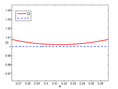
Figure 1: The red solid line represents the value of $Q$. When $\frac{1}{50}(25-\sqrt{141})\leq a\leq\frac{1}{100}(25+\sqrt{141})$, there is always $Q>1$, which means that this family of quantum states violates Theorem 1.

In the above example, our entanglement criterion and realignment criterion are equally effective, as they both detect all entangled states in this family of quantum states. However, this is not always the case. In general, our criterion is weaker than the realignment criterion because our criterion is derived from the latter.

Example 2. Let us consider the Werner state,

$$\rho_{u}=u|\psi\rangle\langle\psi|+\frac{1-u}{4}I_{4},$$

where $0\leq u\leq 1$, $|\psi\rangle=\frac{1}{\sqrt{2}}(|00\rangle+|11\rangle)$ and $I_{4}$ is the $4\times 4$ identity matrix. By calculation it can be concluded that $Q>1$ when $u>0.54$, which means that entanglement of $\rho_{u}$ can be detected by our entanglement criterion within the range of $0.54<u\leq 1$. However, according to the realignment criterion $\rho_{u}$ is entangled when $u>\frac{1}{3}$. This also indicates that in order to achieve the experimental feasibility, our criterion is weaker than the original realignment criterion.

III III. Separability criterion based on PT moments

With respect to the partially transposed matrix $\rho^{\tau}$ of $\rho$, the PT moments are defined as

$T^{\tau}_{k}=Tr[(\rho^{\tau})^{k}],~{}~{}~{}k=1,2,...,mn.$

Consider the characteristic polynomial of $\rho^{\tau}$,

$a_{0}\lambda^{p}-a_{1}\lambda^{p-1}+...+(-1)^{p-1}a_{p-1}\lambda+(-1)^{p}a_{p}$,

where $p=mn$ is the number of rows of the matrix $\rho^{\tau}$, $a_{0}=1$, $a_{k}=\sum_{\{s_{k}\}\in S}\prod_{j\in s_{k}}\lambda_{j}$, $k=1,2,...,p,$ ${s_{k}}$ denotes a subset of $S=\{1,2,...,p\}$ with $k$ elements. The characteristic polynomial coefficients and the PT moments have the following relations jfjq ,

$$a_{k+1}=\frac{1}{k+1}\sum_{l=0}^{k}(-1)^{l}a_{k-l}T^{\tau}_{l+1}$$ (6)

for $k=0,1,...,p-1$. We have the following result.

Theorem 2.

If the bipartite state $\rho$ is separable, then

$$a_{k}\,a_{k+1}>0,~{}~{}~{}k=0,1,...,q-1,$$ (7)

where $q$ is the rank of the matrix $\rho^{\tau}$, $a_{k}$ is given in Eq.(6), with $a_{q}\neq 0$ and $a_{r}=0$ for $r>q$.

Proof.

The characteristic polynomial of $\rho^{\tau}$ can be rewritten as $P(\lambda)=a_{0}\lambda^{p}-a_{1}\lambda^{p-1}+...+(-1)^{q}a_{q}\lambda^{p-q}.$ We first prove that $\rho^{\tau}$ is positive semidefinite if and only if $a_{k}a_{k+1}>0$ for each $k=0,...,q-1$. If $a_{k}a_{k+1}>0$ for each $k=0,...,q-1$, since $a_{0}=1$ the symbols of the coefficients of the characteristic polynomial are strictly alternating. Thus $P(\lambda)$ has no negative roots. Otherwise, if we assume the existence of negative roots, we obtain contradictions. Hence $\rho^{\tau}$ has only nonnegative eigenvalues.

Conversely, if $\rho^{\tau}$ is positive semidefinite, we denote its positive eigenvalues by $\lambda_{1},...,\lambda_{q}$, with all the remaining $p-q$ eigenvalues being $0$. Through inductive argument, we obtain that the signs of the coefficients of the polynomials $(\lambda-\lambda_{1})(\lambda-\lambda_{2})...(\lambda-\lambda_{q})$ alternate strictly, which gives $P(\lambda)$ up to a factor $\lambda^{p-q}$. Therefore, $\rho^{\tau}$ is positive semidefinite if and only if $a_{k}a_{k+1}>0$ for each $k=0,...,q-1$. From the PPT criterion that $\rho^{\tau}$ is positive semidefinite for any bipartite separable state $\rho$, we complete the proof of Theorem 2.         

Theorem 2 implies that if a bipartite quantum state violates any inequality in Eq.(7), it must be entangled. From the proof of Theorem 2, it is seen that our criterion is equivalent to the PPT criterion. However, the PPT criterion can not be applied without state tomography. Our criterion can be used to detect the entanglement of unknown quantum states. We only need to measure the PT moments, since the conditions $a_{k}a_{k+1}>0$, $k=0,1,...,m-1$, in the Theorem 2 can be transformed into the relationship among the moments. We illustrate the usefulness of our criterion through the following example.

Example 3. Consider the two-qubit isotropic state given in zlfw ,

$$\rho_{b}=\frac{1-b}{3}I_{2}\otimes I_{2}+\frac{4b-1}{3}|\psi\rangle\langle\psi|,~{}~{}0\leq b\leq 1,$$

where $I_{2}$ denotes the second-order identity matrix, $|\psi\rangle=\frac{1}{\sqrt{2}}(|00\rangle+|11\rangle)$. We have

$$T^{\tau}_{1} =1,$$

$$T^{\tau}_{2} =\frac{1}{3}(4b^{2}-2b+1),$$

$$T^{\tau}_{3} =-\frac{8}{9}b^{3}+\frac{5}{3}b^{2}-\frac{2}{3}b+\frac{5}{36},$$

$$T^{\tau}_{4} =\frac{84}{81}b^{4}-\frac{156}{81}b^{3}+\frac{126}{81}b^{2}-\frac{39}{81}b+\frac{21}{324}.$$

Substituting the above moments into the inequalities in Theorem 2, we obtain that $\rho_{b}$ is entangled when $b>0.5$, which is exactly the same result as the one from the realignment and PPT criterion directly, and stronger than the result $b\geq 0.608594$ given in ssa .

IV IV. Experimentally measurable lower bound of concurrence

For any $m\otimes n$ $(m\leq n)$ quantum state $\rho$, Chen et al. proposed a lower bound of concurrence csf ,

$$C(\rho)\geq\sqrt{\frac{2}{m(m-1)}}\max(\|\rho^{\tau}\|-1,\|\rho^{R}\|-1).$$ (8)

To obtain experimentally measurable lower bound of concurrence, we next derive the lower bounds according to the moments from $\|\rho^{\tau}\|$ and $\|\rho^{R}\|$.

Theorem 3.

For any $m\otimes n(m\leq n)$ quantum state $\rho$, we have the following experimentally measurable lower bound of concurrence,

$$C(\rho)\geq\sqrt{\frac{2}{m(m-1)}}\max\{M_{1},M_{2},0\},$$ (9)

where

$$M_{1}=\sqrt{\sqrt{2[(T_{1})^{2}-T_{2}]}+T_{1}}-1,$$

$$M_{2}=\sqrt{\sqrt{2[(T^{R}_{1})^{2}-T^{R}_{2}]}+T^{R}_{1}}-1$$

with $T_{i}=Tr[(\rho^{\tau\dagger}\rho^{\tau})^{i}]$ and $T^{R}_{i}=Tr[(\rho^{R\dagger}\rho^{R})^{i}]$, $i=1,2$.

Proof.

Firstly, we have proven that if $\rho$ is a separable state, then $M_{1}\leq 0$. Similar to the proof of Theorem 1, we have $\|\rho^{\tau}\|\geq\sqrt{\sqrt{2[(T_{1})^{2}-T_{2}]}+T_{1}}$. Hence we only need to prove that $\|\rho^{\tau}\|\leq 1$. Since $\rho$ is separable, the eigenvalues $\xi_{i}$ of $\rho^{\tau}$ are non negative and the summation of the eigenvalues is $1$, $\sum_{i}\xi_{i}=1$, $\xi_{i}\geq 0$, $i=1,2,...,mn$. Hence the eigenvalues of $\rho^{\tau\dagger}\rho^{\tau}$ are $\xi^{2}_{i}$ $(i=1,2,...,mn)$. As the singular values of $\rho^{\tau}$ are the arithmetic square root of the non negative eigenvalues of $\rho^{\tau\dagger}\rho^{\tau}$, we have $\|\rho^{\tau}\|=\sum_{i}\xi_{i}=1$. From the definition of concurrence and the formula (8), we obtain Eq.(9).         

Example 4. Consider the following $3\times 3$ dimensional quantum states

$$\rho_{s}=\frac{1-s}{9}I_{9}+s|\psi_{3}\rangle\langle\psi_{3}|,~{}~{}s\in[0,1],$$

where $|\psi_{3}\rangle=\frac{1}{\sqrt{3}}\sum_{i=1}^{3}|ii\rangle$. The state is shown to entangled for $s>\frac{1}{4}$ mhph . From Theorem 3 we obtain the experimental measurable lower bound, which detects most of the entangled states in this family, see Figure. 2.

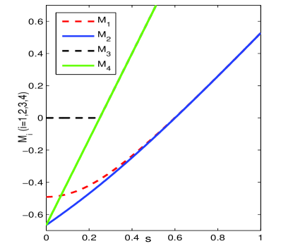
Figure 2: The red dashed line represents the value of $M_{1}$, the blue solid line denotes the value of $M_{2}$, the value of $\|\rho^{\tau}\|-1$ is represented by a black dashed line $M_{3}$, and the value of $\|\rho^{R}\|-1$ is represented by a green solid line $M_{4}$. For $s>0.5994$ the maximum values of $M_{1}$ and $M_{2}$ are greater than 0.

V V. Entanglement measure based on moments of reduced states

Let $|\psi_{AB}\rangle=\sum_{i=1}^{d}\sqrt{\mu_{i}}|ii\rangle$ be a bipartite pure state in $H_{A}\otimes H_{B}$ in Schmidt decomposition, where $\sum_{i=1}^{d}\mu_{i}=1$, $\mu_{i}\geq 0$ $(i=1,2,...,d)$ and $d=\min(m,n)$ with $m$ and $n$ the dimensions of $H_{A}$ and $H_{B}$, respectively. Consider the characteristic polynomial of the reduced density matrix $\rho_{A}$ of $|\psi_{AB}\rangle$,

$$b_{0}\mu^{m}-b_{1}\mu^{m-1}+...+(-1)^{m-1}b_{m-1}\mu+(-1)^{m}b_{m},$$ (10)

where $b_{0}=1$,

$$b_{k}=\sum_{\{g_{k}\}\in G}\prod_{j\in g_{k}}\mu_{j},~{}~{}k=1,2,...,m,$$ (11)

with ${g_{k}}$ a subset of $G=\{1,2,...,m\}$ of $k$ elements.

The coefficients of the characteristic polynomial of a reduced density matrix for a bipartite pure state can be linearly expressed by the moments of the reduced density matrix jfjq ,

$$b_{k+1}=\frac{1}{k+1}\sum_{l=0}^{m}(-1)^{l}b_{k-l}Tr(\rho^{l+1}_{A}),$$ (12)

where $b_{0}=1$ and $k=0,1,...,m-1$. Hence, as the entanglement can be usually characterized by the reduced density matrix wkw ; xmys ; zwms ; zwsm , it can be also quantified by the moments of the reduced density matrix. We define the following entanglement measure based on moments of the reduced states (EMMRS),

$$E^{rm}(|\psi_{AB}\rangle)= 1-\displaystyle\sum_{i=1}^{\frac{m}{2}}[\frac{4i}{m^{2}+2m}Tr(\rho^{i}_{A})$$

$$+\displaystyle\frac{2m-4i+4}{m^{2}+2m}Tr(\rho^{i+\frac{m}{2}}_{A})]$$

for even $m$, and

$$E^{rm}(|\psi_{AB}\rangle) = 1-\sum_{i=1}^{\frac{m-1}{2}}[\frac{4i}{(m+1)^{2}}Tr(\rho^{i}_{A})$$

$$+ \frac{2m-4i+2}{(m+1)^{2}}Tr(\rho^{\frac{m+1}{2}+i}_{A})-\frac{2}{m+1}Tr(\rho^{\frac{m+1}{2}}_{A})]$$

for odd $m$.

The EMMRS for general mixed states $\rho_{AB}$ is given by convex-roof extension,

$$E^{rm}(\rho_{AB})=\mathop{\min}_{\{p_{i},|\psi_{i}\rangle_{AB}\}}\sum_{i}p_{i}E^{rm}(|\psi_{i}\rangle_{AB}),$$ (13)

where the minimization goes over all possible pure state decompositions of $\rho_{AB}=\sum_{i}p_{i}|\psi_{i}\rangle_{AB}\langle\psi_{i}|$.

Before presenting our main results, we first prove two lemmas.

Lemma 1.

For any ensemble $\{p_{i},\rho_{i}\}$ of a quantum state $\rho$, we have

$$Tr[(\sum_{i}p_{i}\rho_{i})^{n}]\leq\sum_{i}p_{i}Tr(\rho^{n}_{i}).$$ (14)

Proof.

We first prove the case for $i=2$, $\rho=p_{1}\rho_{1}+p_{2}\rho_{2}$, where $p_{1}+p_{2}=1$. For $n\geq 2$, we have

$$Tr(p_{1}\rho_{1}+p_{2}\rho_{2})^{n} \leq \{[Tr(p_{1}\rho_{1})^{n}]^{\frac{1}{n}}+[Tr(p_{2}\rho_{2})^{n}]^{\frac{1}{n}}\}^{n}$$

$$= \{p_{1}[Tr(\rho_{1}^{n})]^{\frac{1}{n}}+p_{2}[Tr(\rho_{2}^{n})]^{\frac{1}{n}}\}^{n}$$

$$\leq p_{1}Tr(\rho^{n}_{1})+p_{2}Tr(\rho^{n}_{2}),$$

where the first inequality is due to the Minkowski inequality, the second inequality is due to the convexity of the function $y=x^{n}$ when $x$ is non negative. By using mathematical induction, we can obtain inequality (14).         

Lemma 2.

For any ensemble $\{p_{i},\rho_{i}\}$ of a quantum state $\rho$, denote

$$f(\rho)=1-\sum_{i=1}^{\frac{m}{2}}[\frac{4i}{m^{2}+2m}Tr(\rho^{i})+\frac{2m-4i+4}{m^{2}+2m}Tr(\rho^{i+\frac{m}{2}})]$$

for even $m$ and

$$g(\rho) = 1-\sum_{i=1}^{\frac{m-1}{2}}[\frac{4i}{(m+1)^{2}}Tr(\rho^{i})$$

$$+ \frac{2m-4i+2}{(m+1)^{2}}Tr(\rho^{\frac{m+1}{2}+i})$$

$$- \frac{2}{m+1}Tr(\rho^{\frac{m+1}{2}})]$$

for odd $m$. We have

$$f(\rho) \geq \sum_{i}p_{i}f(\rho_{i}),$$ (15)

$$g(\rho) \geq \sum_{i}p_{i}g(\rho_{i}).$$ (16)

Proof.

By definition we have

$$f(\rho) = f(\sum_{j}p_{j}\rho_{j})$$

$$= 1-\sum_{i=1}^{\frac{m}{2}}[\frac{4i}{m^{2}+2m}Tr[(\sum_{j}p_{j}\rho_{j})^{i}]$$

$$+ \frac{2m-4i+4}{m^{2}+2m}Tr[(\sum_{j}p_{j}\rho_{j})^{i+\frac{m}{2}}]]$$

$$\geq 1-\sum_{j}p_{j}\sum_{i=1}^{\frac{m}{2}}[\frac{4i}{m^{2}+2m}Tr(\rho_{j})^{i}+\frac{2m-4i+4}{m^{2}+2m}Tr(\rho_{j})^{i+\frac{m}{2}}]$$

$$= \sum_{j}p_{j}f(\rho_{j}),$$

where the inequality is due to Lemma 1. Similarly, we can prove the inequality (16).         

We are now ready to present a bona fide measure of quantum entanglement. In fact, a well-defined quantum entanglement measure must satisfy the conditions vmmp ; vvmbp ; gvrt as follows:

(i) $E(\rho)\geq 0$ for any quantum state $\rho$ and $E(\rho)=0$ if $\rho$ is separable.

(ii) $E$ is invariant under local unitary transformation.

(iii) $E$ does not increase on average under stochastic LOCC.

(iv) $E$ is convex.

(v) $E$ cannot increase under LOCC, that is, $E(\rho)\geq E(\Lambda(\rho))$ for any LOCC map $\Lambda$.

It has been proposed in wlf that a covex function $E$ satisfies conditions (v) if and only if it satisfies conditions (ii) and (iii). $E$ is said to be an entanglement monotonegvid if the first four conditions hold. From this point of view any entanglement monotone defined in gvid could be regarded as a measure of entanglement.

Theorem 4.

For any state $\rho_{AB}$, $E^{rm}(\rho_{AB})$ is a well-defined measure of quantum entanglement.

Proof.

Firstly, we prove that if $|\psi_{AB}\rangle$ is a separable pure state, then $E^{rm}(|\psi_{AB}\rangle)=0$. If $|\psi_{AB}\rangle$ is a separable state, its reduced density matrix $\rho_{A}$ is pure. The moment of any order of $\rho_{A}$ is equal to $1$, that is, $Tr(\rho^{k}_{A})=1$, $k=1,2,...$. Thus

$$E^{rm}(|\psi_{AB}\rangle)=1-\sum_{i=1}^{\frac{m}{2}}\frac{4i}{m^{2}+2m}+\frac{2m-4i+4}{m^{2}+2d}=0.$$

This equation also indicates that when the pure state $|\psi_{AB}\rangle$ is not separable, its reduced state $\rho_{A}$ is a mixed state, therefore $Tr(\rho^{k}_{A})<1$, for $k=1,2,...$. That is $E^{rm}(|\psi_{AB}\rangle)>0$. For mixed state $\rho$, by definition and proof of the pure state case, $E^{rm}(\rho_{AB})\geq 0$, and if $\rho_{AB}$ is separable, $E^{rm}(\rho_{AB})=0$.

$E$ is invariant under local unitary transformations from the invariance of $Tr(\rho^{i})$.

Below we prove that $E^{rm}(\rho)$ is non-increasing on average under LOCC. Let $|\psi_{AB}\rangle$ be a bipartite pure state, and $\{\eta_{i}\}$ be a completely positive trace preserving map on the subsystem $B$. Then the post-mapped state is

$$\sigma_{i}=\frac{1}{p_{i}}\eta_{i}(\sigma),$$

where $\sigma=|\psi\rangle_{AB}\langle\psi|$ and $p_{i}=Tr(\eta_{i}\sigma)$. Let $\sigma^{A}_{i}=Tr_{B}(\sigma_{i})$. We have

$$\sigma^{A}=\sum_{i}p_{i}\sigma^{A}_{i}.$$

Let $\{p_{ij},\sigma_{ij}\}$ be the optimal ensemble of $\sigma_{i}$ such that

$$E^{rm}(\sigma_{i})=\sum_{j}p_{ij}E^{rm}(\sigma_{ij}),$$

where $\{\sigma_{ij}\}$ are pure states. Thus,

$$E^{rm}(\rho) = f(\sigma^{A})$$ (17)

$$= f(\sum_{i,j}p_{i}p_{ij}\sigma^{A}_{ij})$$

$$\geq \sum_{i,j}p_{i}p_{ij}f(\sigma^{A}_{ij})$$

$$= \sum_{i,j}p_{i}p_{ij}E^{rm}(\sigma_{ij})$$

$$= \sum_{i}p_{i}E^{rm}(\sigma_{i}),$$

where $\sigma^{A}_{ij}=Tr_{B}(\sigma_{ij})$ and the inequality is due to Lemma 2.

Now, for any mixed quantum state $\rho$, let $\{\varepsilon_{i}\}$ be a completely positive trace preserving map. Then the post-mapped state is

$$\rho_{i}=\frac{1}{\pi_{i}}\varepsilon_{i}(\rho),$$

where $\pi_{i}=Tr(\varepsilon_{i}\rho)$. Suppose $\{q_{j},|\psi_{j}\rangle\}$ be the optimal pure-state ensemble of $\rho$. According to the equation (17), we have

$$E^{rm}(|\psi_{j}\rangle)\geq\sum_{i}k_{ji}E^{rm}(\rho_{ji}),$$ (18)

where $k_{ji}=Tr(\varepsilon_{i}|\psi_{j}\rangle\langle\psi_{j}|)$ and $\rho_{ji}=\frac{1}{k_{ji}}\varepsilon_{i}(|\psi_{j}\rangle\langle\psi_{j}|)$. Let $\{k_{jil},|\psi_{jil}\rangle\}$ be the optimal pure-state ensemble of $\rho_{ji}$ such that $E^{rm}(\rho_{ji})=\sum_{l}k_{jil}E^{rm}(|\psi_{jil}\rangle)$. We have

$$E^{rm}(\rho) = \sum_{j}q_{j}E^{rm}(|\psi_{j}\rangle)$$

$$\geq \sum_{j,i}q_{j}k_{ji}E^{rm}(\rho_{ji})$$

$$= \sum_{j,i,l}q_{j}k_{ji}k_{jil}E^{rm}(|\psi_{jil}\rangle)$$

$$\geq \sum_{i}\pi_{i}E^{rm}(\rho_{i}),$$

where the first inequality is due to (18). The last inequality is due to that

$$\rho_{i} = \frac{1}{\pi_{i}}\varepsilon_{i}(\rho)$$

$$= \frac{1}{\pi_{i}}\varepsilon_{i}(\sum_{j}q_{j}|\psi_{j}\rangle\langle\psi_{j}|)$$

$$= \frac{1}{\pi_{i}}\sum_{j}q_{j}\varepsilon_{i}(|\psi_{j}\rangle\langle\psi_{j}|)$$

$$= \frac{1}{\pi_{i}}\sum_{j}q_{j}k_{ji}\rho_{ji}$$

$$= \frac{1}{\pi_{i}}\sum_{j,l}q_{j}k_{ji}k_{jil}|\psi_{jil}\rangle\langle\psi_{jil}|,$$

where in the equality (V), we have used the linear property of $\varepsilon_{i}$.

Finally, we prove convexity. Consider $\rho=t\rho_{1}+(1-t)\rho_{2}$. Let $\rho_{1}=\sum_{i}p_{i}|\psi_{i}\rangle\langle\psi_{i}|$ and $\rho_{2}=\sum_{j}q_{j}|\phi_{j}\rangle\langle\phi_{j}|$ be the optimal pure state decomposition of $E^{rm}(\rho_{1})$ and $E^{rm}(\rho_{2})$, respectively. Where $\sum_{i}p_{i}=\sum_{j}q_{j}=1$ and $p_{i}$, $q_{j}>0$. We have

$$E^{rm}(\rho) \leq \sum_{i}tp_{i}E^{rm}(|\psi_{i}\rangle)+\sum_{j}(1-t)q_{j}E^{rm}(|\phi_{j}\rangle)$$

$$= tE^{rm}(\rho_{1})+(1-t)E^{rm}(\rho_{2}),$$

where the inequality is due to that $\sum_{i}tp_{i}|\psi_{i}\rangle\langle\psi_{i}|+\sum_{j}(1-t)q_{j}|\phi_{j}\rangle\langle\phi_{j}|$ is also a pure state decomposition of $\rho$.         

To demonstrate the usefulness of EMMRS, let us consider the family of $3\times 3$ quantum states given in Example 1. From our EMMRS we obtain

$$E^{rm}(\rho_{a})=\frac{5}{32}a^{2}-\frac{5}{32}a+\frac{15}{16}.$$

The value of $E^{rm}(\rho_{a})$ is always greater than 0 for $a\in[\frac{1}{50}(25-\sqrt{141}),\frac{1}{100}(25+\sqrt{141})]$, decreasing with the increase of $a$, see Figure. 3. It is worth noting that in ga , the singlet fraction $F^{max}(\rho_{a})$, which is directly related to the ability of quantum teleportation, also decreases with the increase of $a$. Hence, our entanglement measure also reflects the ability of the state in quantum teleportation.

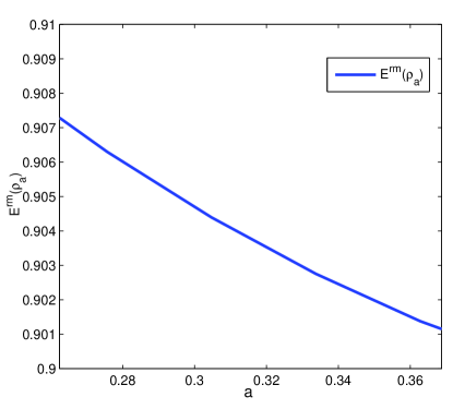
Figure 3: $E^{rm}(\rho_{a})>0$ for $a\in[\frac{1}{50}(25-\sqrt{141}),\frac{1}{100}(25+\sqrt{141})]$, and $E^{rm}(\rho_{a})$ decreases with the increase of $a$.

From the definition of EMMRS, we see that for $m=2$, $E^{rm}(|\psi_{AB}\rangle)=\frac{1}{2}(1-Tr(\rho^{2}_{A}))=\frac{C^{2}(|\psi_{AB}\rangle)}{4}$, which is just the square of concurrence up to a constant factor. When $m$ increases our entanglement measure can traverse all the moments of the reduced density matrix $\rho_{A}$, thus capturing relatively complete information on the entanglement properties of quantum states.

Example 5. We consider the following rank-3 states given in jfjq ,

$$|\phi_{1}\rangle_{AB} = \frac{1}{\sqrt{2}}|00\rangle+\frac{1}{\sqrt{3}}|11\rangle+\frac{1}{\sqrt{6}}|22\rangle,$$

$$|\phi_{2}\rangle_{AB} = \sqrt{\beta_{1}}|00\rangle+\sqrt{\beta_{2}}|11\rangle+\sqrt{1-\beta_{1}-\beta_{2}}|22\rangle,$$

where $\beta_{1}=\frac{1}{4}$ and $\beta_{2}=\frac{9+\sqrt{13}}{24}$. The concurrences of these two quantum states are equal, $C(|\phi_{1}\rangle_{AB})=C(|\phi_{2}\rangle_{AB})$. However, using our EMRM we obtain $E^{rm}(|\phi_{1}\rangle_{AB})=0.5139$ and $E^{rm}(|\phi_{2}\rangle_{AB})=0.5126$. This indicates that although both $|\phi_{1}\rangle_{AB}$ and $|\phi_{2}\rangle_{AB}$ are entangled states, the degree of entanglement is different. Our entanglement measure can characterize the entanglement in a more fine way.

VI VI. Genuine tripartite entanglement measure based on EMMRS

For a tripartite pure state $|\psi\rangle\in H_{A}\otimes H_{B}\otimes H_{C}$, we define the genuine tripartite entanglement measure (GTE-EMMRS) based on EMMRS,

$$E_{GTE}(|\psi\rangle):=[\prod_{\gamma_{i}\in\Gamma}E^{rm}(|\psi\rangle_{\gamma_{i}})]^{\frac{1}{3}},$$ (20)

where $\Gamma=\{\gamma_{i}\}$ represents the set of all possible bipartitions of $\{A,B,C\}$, and the summation goes over all possible bipartitions $\Gamma=\{(A|B,C),(B|A,C),(C|A,B)\}$. Generalizing to mixed states $\rho$ via a convex roof extension, we have

$$E_{GTE}(\rho)=\mathop{\min}_{\{p_{i},|\psi_{i}\rangle\}}\sum_{i}p_{i}E_{GTE}(|\psi_{i}\rangle),$$ (21)

where the minimum is obtained over all possible pure state decompositions of $\rho=\sum_{i}p_{i}|\psi_{i}\rangle\langle\psi_{i}|$.

In the following we prove that the GTE-EMMRS is a genuine tripartite entanglement measure.

Theorem 5.

The GTE-EMMRS defined in Eq.(21) is a genuine tripartite entanglement measure of tripartite quantum systems.

Proof.

The definition of $E_{GTE}(\rho)$ directly implies $E_{GTE}(\rho)=0$ for all biseparable states and $E_{GTE}(\rho)>0$ for all genuine tripartite entangled states.

Next, we prove convexity. For any mixture $\sum_{i}p_{i}\rho_{i}$, let $\{p_{ij},\rho_{ij}\}$ be the pure-state ensemble of $\rho_{i}$. Thus

$$E_{GTE}(\rho) = E_{GTE}(\sum_{i}p_{i}\rho_{i})$$

$$= E_{GTE}(\sum_{i,j}p_{i}p_{ij}\rho_{ij})$$

$$\leq \sum_{i,j}p_{i}p_{ij}E_{GTE}(\rho_{ij})$$

$$= \sum_{i}p_{i}E_{GTE}(\rho_{i}),$$

where the inequality is due to the definition of $E_{GTE}(\rho)$.

As the EMMRS has been proven to be nonincreasing under LOCC, the geometric mean of EMMRS for all subsystems is also nonincreasing under LOCC. Thus $E_{GTE}(\rho)$ is nonincreasing under LOCC. Therefore, we have completed the proof of the theorem.         

Example 6. Consider the following single parameter family of three-qubit state,

$$\small{\rho_{f}=\frac{1}{4f^{2}+4}\left(\begin{array}[]{cccccccc}1&\frac{1+f^{2}}{4}&\frac{f}{4}&0&0&f&0&1\\ \frac{1+f^{2}}{4}&1&0&0&0&0&0&0\\ \frac{f}{4}&0&2f^{2}&0&0&f^{2}&0&f\\ 0&0&0&0&0&0&0&0\\ 0&0&0&0&0&0&0&0\\ f&0&f^{2}&0&0&2f^{2}&0&\frac{f}{4}\\ 0&0&0&0&0&0&1&\frac{1+f^{2}}{4}\\ 1&0&f&0&0&\frac{f}{4}&\frac{1+f^{2}}{4}&1\\ \end{array}\right),}$$

where $f\in[0,1]$. By calculation, the GME-concurrence presented in mcc has the form,

$$C_{GME}(|\psi\rangle):=\mathop{\min}_{\{\gamma_{i}\in\Gamma\}}\sqrt{2[1-Tr(|\psi\rangle_{\gamma_{i}}^{2})]},$$

which is just a constant, $C_{GME}(\rho_{f})=\sqrt{2[1-Tr(\rho_{f\gamma_{3}})]}=\frac{\sqrt{15}}{4}$ for all $f\in[0,1]$. However, by using our GTE-EMMRS we obtain

$$E_{GTE}(\rho_{f})=\sqrt[3]{\frac{240f^{4}+465f^{2}+240}{16384(1+f^{2})^{2}}}.$$

The genuine tripartite entanglement from our measure depends on the value of $f$. In other words, our entanglement measure GTE-EMMRS effectively distinguishes the genuine tripartite entanglement of this family of quantum states, see Figure. 4. In xe the authors proposed an interesting entanglement measure called the concurrence fill, which is given by the area of a triangle composed of three one-to-other bipartite concurrences serving as side lengths:

$$F_{123}=\frac{4}{\sqrt{3}}\sqrt{P(P-C_{1(23)}^{2})(P-C_{2(13)}^{2})(P-C_{3(12)}^{2})},$$

where $P=\frac{1}{2}(C_{1(23)}^{2}+C_{2(13)}^{2}+C_{3(12)}^{2})$, $C_{i(jk)}$ denotes the concurrence under bipartition $i$ and $jk$. Calculation shows that the concurrence fill decreases with the increase of the parameter $f$. In this sense, GTE-EMMRS and concurrence fill are two inequivalent measures of tripartite entanglement, see Figure. 5.

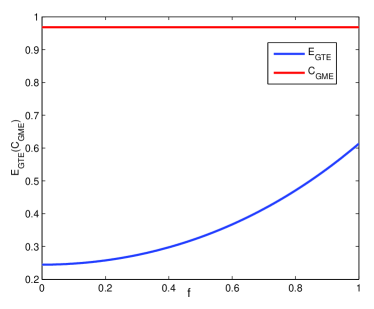
Figure 4: Our entanglement measure $E_{GTE}$ varies with the $f$ for $f\in[0,1]$, while $C_{GME}$ remains unchanged.

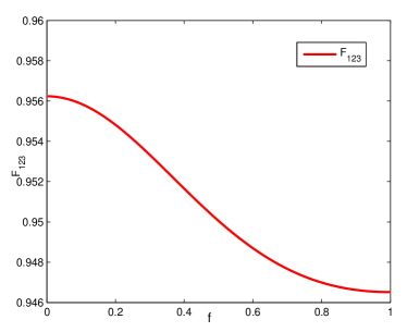
Figure 5: Concurrence fill $F_{123}$ versus $f$ for $f\in[0,1]$.

VII Conclusions and discussions

Based on the moments of the realigned matrix of a density matrix we have proposed an experimentally plausible separability criterion for any dimensional bipartite quantum states. The main advantage of this criterion is that it only requires the first two realignment moments, which simplifies the related experimental measurements. We have also provided a separability criterion based on the relationship between the characteristic polynomial coefficients and the moments of a partially transposed matrix. The discriminant in this criterion can also be represented in terms of PT moments. Therefore, this criterion can also be experimentally implemented. Moreover, we have presented experimentally measurable lower bounds of concurrence for arbitrary bipartite quantum states, which give the ways to determine quantitatively the degree of quantum entanglement without the tomography of unknown quantum states. Based on the moments of the reduced states, we have also obtained a bona fide bipartite entanglement measure. Finally, we have presented a genuine tripartite entanglement measure based on our bipartite entanglement measure, which discriminates entanglement between different quantum states that cannot be distinguished by GME-concurrence.

Acknowledgments:  This work is supported by the Hainan Provincial Natural Science Foundation of China under Grant No.121RC539; the National Natural Science Foundation of China under Grant Nos. 12204137, 12075159 and 12171044; the specific research fund of the Innovation Platform for Academicians of Hainan Province under Grant No. YSPTZX202215; Beijing Natural Science Foundation (Grant No. Z190005) and the Hainan Provincial Graduate Innovation Research Program (Grant No. Qhys2023-386).

Data Availability Statement: This manuscript has no associated data.

References

• (1) A. Einstein, B. Podolsky, N. Rosen, Can quantum mechanical description of physical reality be considered complete? Phys. Rev 47, 777 (1935).
• (2) C.H. Bennett, G. Brassard, C. CrΓ©peau, R. Jozsa, A. Peres, and W. K. Wotters, Teleporting an unknown quantum state via dual classical and Einstein-Podolsky-Rosen channels, Phys. Rev. Lett. 70, 1895 (1993).
• (3) R. Cleve and H. Buhrman, Substituting quantum entanglement for communication, Phys. Rev. A 56, 1201 (1997).
• (4) N. Gigena, R. Rossignoli, Bipartite entanglement in fermion systems, Phys. Rev. A 95, 062320 (2017).
• (5) J. Barrett, Nonsequential positive-operator-valued measurements on entangled mixed states do not always violate a Bell inequality, Phys. Rev. A 65, 042302 (2002).
• (6) S. Lioyd, Universal quantum simulators, Science, 273, 1073 (1996).
• (7) A. Datta, S. T. Flammia and C. M. Caves, Entanglement and the power of one qubit, Phys. Rev. A 72, 042316 (2005).
• (8) A. Ekert and R. Jozsa, Quantum algorithms: Entanglement enhanced information processing, Philos. Trans. R. Soc. A 356, 1769 (1998).
• (9) M. A. Nielsen and I. L. Chuang, Quantum Computation
and Quantum Information (Cambridge University Press, Cambridge, (2000).
• (10) A. K. Ekert, Quantum cryptography based on Bell’s theorem, Phys. Rev. Lett. 67, 661 (1991).
• (11) N. Gisin, G. Ribordy, W. Tittel and H. Zbinden, Quantum cryptography, Rev. Mod. Phys. 74, 145 (2002).
• (12) L. Masanes, Universally composable privacy amplification from causality constraints, Phys. Rev. Lett. 102, 140501 (2009).
• (13) A. Peres, Separability criterion for density matrices, Phys. Rev. Lett. 77, 1413 (1996).
• (14) M. Horodecki, P. Horodecki and R. Horodecki, Separability of n-particle mixed states: necessary and sufficient conditions in terms of linear maps, Phys. Lett. A 223, 1 (1996).
• (15) K. Chen and L.A. Wu, A matrix realignment method for recognizing entanglement, Quantum Inf. Comput. 3(3), 193 (2003).
• (16) O. Rudolph, Further results on the cross norm criterion for separability, Quantum Inf. Process. 4, 219 (2005).
• (17) M. Lewenstein, B. Kraus, J. I. Cirac, and P. Horodecki, Optimization of entanglement witnesses, Phys. Rev. A 62, 052310 (2000).
• (18) R. Horodecki, P. Horodecki, M. Horodecki, and K. Horodecki, Quantum entanglement, Rev. Mod. Phys. 81, 865 (2009).
• (19) O. GΓΌhne, G. TΓ³th, Entanglement detection, Physics Reports 474, 1 (2009).
• (20) S. Imai, N. Wyderka, A. Ketterer and O. GΓΌne, Bound entanglement from randomized measurements, Phys. Rev. Lett. 126, 150501 (2021).
• (21) A. Ketterer, N. Wyderka and O. GΓΌne, Characterizing multipartite entanglement with moments of random correlations, Phys. Rev. Lett. 122, 120505 (2019).
• (22) A. Elben, B. Vermersch, C.F. Roos and P. Zoller, Statistical correlations between locally randomized measurements: a toolbox for probing entanglement in many-body quantum states, Phys. Rev. A 99, 052323 (2019).
• (23) T. Brydges, A. Elben, P. Jurceive, B. Vermersch, C. Maier, B.P. Lanyon, P. Zoller, R. Blatt and C.F. Roos, Probing renyi entanglement entropy via randomized measurements, Science 364, 260 (2019).
• (24) L. Knips, J. Dziewior, W. Klobus, W. Laskowski, T. Paterek, P.J. Shadbolt, H. Weinfurter and J.D.A. Meinecke, Multipartite entanglement analysis from random correlations, npj Quantum Inf. 6, 51 (2020).
• (25) X. Yang, M.X. Luo, Y.H. Yang, and S.M. Fei, Parametrized entanglement monotone, Phys. Rev. A 103, 052423 (2021).
• (26) Z.W. Wei, M.X. Luo, S.M. Fei, Estimating parameterized entanglementmeasure, Quantum Inf. Process. 21, 210 (2022).
• (27) Z.W. Wei and S.M. Fei, Parameterized bipartite entanglement measure, J. Phys. A: Math. Theor. 55, 275303 (2022).
• (28) Z.X. Jin, S.M. Fei, X. Li-Jost and C.F. Qiao, Informationally complete measures of quantum entanglement, Phys. Rev. A 107, 012409 (2023).
• (29) H. Li, T. Gao, F. Yan, Parameterized multipartite entanglement measures, arXiv:2308.16393, (2023).
• (30) F. Bohnet-Waldraff, D. Braun and O. Giraud, Entanglement and the truncated moment problem, Phys. Rev. A 96, 032312 (2017).
• (31) A. Elben, R. Kueng, H. Y. R. Huang, R. van Bijnen, C. Kokail, M. Dalmonte, P. Calabrese, B. Kraus, J. Preskill, P. Zoller and B. Vermersch, Mixed-state entanglement from local randomized measurements, Phys. Rev. Lett. 125, 200501 (2020).
• (32) X.D. Yu, S. Imai, O. Guhne, Optimal entanglement certification from moments of the partial transpose, Phys. Rev. Lett 127, 060504 (2021).
• (33) Y. Zhou, P. Zeng and Z. Liu, Single-copies estimation of entanglement negativity, Phys. Rev. Lett 125, 200502 (2020).
• (34) J. Gray, L. Banchi, A. Bayat and S. Bose, Machine-learning-assisted many-body entanglement measurement, Phys. Rev. Lett. 121, 150503 (2018).
• (35) H.Y. Huang, R. Kueng and J. Preskill, Predicting many properties of a quantum system from very few measurements, Nat. Phys. 16, 1050 (2020).
• (36) A. Neven, J. Carrasco, V. Vitale, C. Kokail, A. Elben, M. Dalmonte, P. Calabrese, P. Zoller, B. Vermersch, R. Kueng and B. Kraus, Symmetry-resolved entanglement detection using partial transpose moments, Npj Quantum Inf. 7, 152 (2021).
• (37) T. Zhang, N. Jing, and S.M. Fei, Quantum separability criteria based on realignment moments, Quantum Inf. Process. 21, 276 (2022).
• (38) K.K. Wang, Z.W. Wei, S.M. Fei, Operational entanglement detection based on $\Lambda$-moments, Eur. Phys. J. Plus 137, 1378 (2022).
• (39) Z. Liu, Y. Tang, H. Dai, P. Liu, S. Chen, and X. Ma, Detecting entanglement in quantum many-body systems via permutation moments, Phys. Rev. Lett. 129, 260501 (2022).
• (40) M. Ali, Partial transpose moments, principal minors and entanglement detection, Quantum Inf. Process. 22, 207 (2023).
• (41) S. Aggarwal, A. Kumari, and S. Adhikari, Physical realization of realignment criteria using the structural physical approximation, Phys. Rev. A 108, 012422 (2023).
• (42) S. Aggarwal, S. Adhikari, A. S. Majumdar, Entanglement detection in arbitrary dimensional bipartite quantum systems through partial realigned moments, Phys. Rev. A109, 012404 (2024).
• (43) N. Friis, G. Vitagliano, M. Vitagliano, M. Huber, Entanglement certification from theory to experiment. Nat. Rev. Phys. 1, 72 (2019).
• (44) W. K. Wootters, Entanglement of formation of an arbitrary state of two qubits, Phys. Rev. Lett. 80, 2245 (1998).
• (45) G. Vidal, R. F. Werner, Computable measure of entanglement, Phys. Rev. A 65, 032314 (2002).
• (46) C. Simon, J. Kempe, Robustness of multiparty entanglement, Phys. Rev. A 65, 052327 (2002).
• (47) F. Mintert, M. Kus and A. Buchleitner, Concurrence of mixed multi-partite quantum states, Phys. Rev. Lett. 95, 260502 (2005).
• (48) Z.H. Ma, Z.H. Chen, J.L. Chen , C. Spengler, A. Gabriel and M. Huber, Measure of genuine multipartite entanglement with computable lower bounds, Phys. Rev. A 83, 062325 (2011).
• (49) S. Xie and J. H. Eberly, A triangle governs genuine tripartite entanglement, Phys. Rev. Lett. 127, 040403 (2021).
• (50) C. Emary and C. W. J. Beenakker, Relation between entanglement measures and Bell inequalities for three qubits, Phys. Rev. A 69, 032317 (2004).
• (51) D. Sadhukhan, S. S. Roy, A. K. Pal, D. Rakshit, A. Sen(De), U. Sen, Multipartite entanglement accumulation in quantum states: Localizable generalized geometric measure, Phys. Rev. A 95, 022301 (2017).
• (52) A. Sen(De) and U. Sen, Channel capacities versus entanglement measures in multiparty quantum states, Phys. Rev. A 81, 012308 (2010).
• (53) S. M. Hashemi Rafsanjani, M. Huber, C. J. Broadbent and J. H. Eberly, Genuinely multipartite concurrence of N-qubit X matrices, Phys. Rev. A 86, 062303 (2012).
• (54) Y. Guo, Y. Jia, X. Li and L. Huang, Genuine multipartite entanglement measure, J. Phys. A: Math. Theor. 55, 145303 (2021).
• (55) Z.X. Jin, Y.H. Tao, Y.T. Gui, S.M. Fei, X. Li-Jost and C.F. Qiao, Concurrence triangle induced genuine multipartite entanglement measure, Results in Physics. 44, 106155 (2022).
• (56) A. Grag, S. Adhikari, Teleportation criteria based on maximum eigenvalue of the shared $d\otimes d$ dimensional mixed state: beyond singlet fraction, Int. J. Theor. Phys. 60, 1038 (2021).
• (57) M.J. Zhao, Z.G. Li, S.M. Fei and Z.X. Wang, A note on fully entangled fraction, J. Phys. A: Math. Theor. 43, 275203 (2010).
• (58) K. Chen, S. Albeverio and S.M. Fei, Concurrence of arbitrary dimensional bipartite quantum states, Phys. Rev. Lett. 95, 040504 (2005).
• (59) M. Horodecki and P. Horodecki, Reduction criterion of separability and limits for a class of distillation protocols, Phys. Rev. A 59, 040504 (2005).
• (60) V. Vidal, M. B. Plenio, M. A. Rippin and P. L. Knight, Quantifying entanglement, Phys. Rev. Lett. 78, 2275 (1997)
• (61) V. Vidal and M. B. Plenio, Entanglement measures and purification procedures, Phys. Rev. A. 57, 1619 (1998)
• (62) G. Vidal and R. Tarrach, Robustness of entanglement, Phys. Rev. A. 59, 141 (1999)
• (63) Z.W. Wei, M.X. Luo and S.M. Fei, Estimating parameterized entanglement measure, Quantum Inf. Process. 21, 210 (2022)
• (64) G. Vidal, Entanglement monotones, J. Mod. Optics 47, 355 (2000).