HILCodec: High Fidelity and Lightweight Neural Audio Codec

Abstract

The recent advancement of end-to-end neural audio codecs enables compressing audio at very low bitrates while reconstructing the output audio with high fidelity. Nonetheless, such improvements often come at the cost of increased model complexity. In this paper, we identify and address the problems of existing neural audio codecs. We show that the performance of Wave-U-Net does not increase consistently as the network depth increases. We analyze the root cause of such a phenomenon and suggest a variance-constrained design. Also, we reveal various distortions in previous waveform domain discriminators and propose a novel distortion-free discriminator. The resulting model, HILCodec, is a real-time streaming audio codec that demonstrates state-of-the-art quality across various bitrates and audio types.

I Introduction

An audio codec is a system that compresses and decompresses audio data. It comprises an encoder which analyzes the input audio, a quantizer, and a decoder that reconstructs the output audio. Audio codecs have several objectives. First, they aim to compress the input using the minimum number of bits. Second, they strive to preserve the perceptual quality of the output, making it as similar as possible to the original input. Third, they seek to maintain a low delay for streaming applications. Lastly, they are designed to have low computational complexity so that they can be used on a variety of devices, including mobile and embedded systems.

Traditional audio codecs leverage the expertise of speech processing, audio signal processing, and psychoacoustics to achieve their objectives. For speech coding, based on the source-filter model of speech production [2], linear predictive coding (LPC) [3] is widely adopted because of its high compression rate. Instead of compressing the waveform directly, LPC represents the input speech as an autoregressive model and quantizes the model’s coefficients. These coefficients are then dequantized and used to synthesize the output speech. However, LPC is not good at capturing high frequency components. Therefore, for other types of audios, such as music, transform coding is employed [4, 8, 11]. This method first transforms the input waveform into another domain, such as subbands [13], wavelet coefficients [15], or a time-frequency spectrogram [14], to obtain less correlated components. It then allocates available bits so that quantization noise for each component is psychoacoustically well-distributed [12]. Finally the decoder applies an inverse transform to obtain the output waveform.

Recently, the remarkable advancements of machine learning have spurred active research into audio coding based on deep neural networks (DNNs). One research direction involves using a DNN as a post-processing enhancement module for existing codecs to suppress coding artifacts at low bitrates [30, 31, 32]. In some studies, a DNN decoder is trained on top of a traditional human-designed encoder. The input for such neural decoder can be the output representations of an encoder after quantization [33, 35], or the raw bitstream itself [34]. Another promising area is an end-to-end neural audio codec [36, 37, 38, 39, 42, 40, 41], where instead of relying on manually designed encoders and quantizers, the entire encoder-quantizer-decoder framework is trained in a data-driven way. Leveraging the power of generative adversarial networks (GAN) [43], end-to-end neural audio codecs have demonstrated state-of-the-art audio quality under low bitrate conditions. On the other hand, these improvements in audio quality are often attributed to an increase in network size, leading to substantial computational complexity. Furthermore, some of these codecs are not streamable. While there exist neural audio codecs that can be processed in real time streaming manner, it results in compromised performance. Given the growing demand and potential for neural audio codecs in real-world services, the development of a codec that is lightweight, streamable, and maintains high fidelity presents a timely and valuable opportunity.

In this paper, we challenge the common practice of simply augmenting model complexity. Our main focus is on dissecting and addressing the issues discovered from the existing generators and discriminators which hinder model performance. Combined with a lightweight backbone network, we propose HILCodec, an end-to-end neural audio codec that satisfies the aforementioned requirements. It is capable of compressing diverse types of audio data at bitrates ranging from 1.5 kbps to 9.0 kbps, with a sampling rate of 24kHz. HILCodec can operate in real-time on a single thread of a CPU while demonstrating comparable or superior audio quality to other traditional and neural audio codecs.

For the generator, we construct a low-complexity version of the widely-used Wave-U-Net architecture [16] using depthwise-separable convolutions [51]. We incorporate $L_{2}$-normalization and multi-resolution spectrogram inputs, which enhance the model’s performance with a minimal increase in computational complexity. These modifications serves us a room to increase the width and depth of the network.

However, we identify an issue of the Wave-U-Net architecture where an increase in network depth does not always leads to an improvement in audio quality and may even result in quality degradation. This problem has not been addressed explicitly in previous studies on audio coding. Through theoretical and empirical analysis, we deduce that the discrepancy is due to the exponential increase in variance of activations during the forward pass. To mitigate this, we propose a variance-constrained design, which effectively scales performance in line with network depth.

In addition, we show that existing waveform domain discriminators often operate on distorted signals. As a solution, we introduce a distortion-free discriminator that utilizes multiple filter banks to enhance perceptual quality. When combined with a time-frequency domain discriminator, it surpasses the performance of conventional discriminators in GAN-based audio codecs in terms of subjective quality. These innovative approaches significantly contribute to the overall effectiveness of our proposed HILCodec.

Our main contributions are summarized as follow:

• We propose a lightweight generator backbone architecture that runs on devices with limited resources.

• We identify a problem associated with the Wave-U-Net generator: increasing network depth does not necessarily lead to improved performance. We address this by adopting a variance-constrained design.

• Based on signal processing theories, we propose a distortion-free multi-filter bank discriminator (MFBD).

• We compare HILCodec against the state-of-the-art traditional codec and neural audio codecs across various bitrates and audio types. The evaluation results demonstrate that our model matches or even surpasses the performance of previous codecs, even with reduced computational complexity.

Audio samples, code, and pre-trained weights are publicly available.

II Related Works

II-A Neural Vocoder

A vocoder is a system that synthesizes human voice from latent representations. The study on vocoders originated from [1] and has since been central to digital speech coding. Recently, neural vocoders have brought significant attention due to their applicability to text-to-speech (TTS) systems. A neural vocoder synthesizes speech from a given mel-spectrogram, while a separate neural network generates the mel-spectrogram from text. Various neural vocoders have been proposed based on deep generative models, including autoregressive models [18, 20, 19], flow [21], diffusion [25, 26], and others. Among these, vocoders based on the GAN framework have been popular due to their high-quality output and fast inference time. MelGAN [22] introduced the Multi-Scale Discriminator (MSD) which operates on average-pooled waveform and a feature matching loss to stabilize adversarial training. Parallel WaveGAN [23] introduced a multi-resolution short-time Fourier transform (STFT) loss, which outperforms the single-resolution counterpart. HiFi-GAN [24] proposed a well-designed generator and Multi-Period Discriminator (MPD) which operates on downsampled waveform. Avocodo [27] aimed to reduce aliasing in the generator and waveform domain discriminators by introducing the Cooperative Multi-Band Discriminator (CoMBD) and Subband Discriminator (SBD). Some models used time-frequency domain discriminators [28, 29]. Due to the similarity of the tasks, developments in the field of neural vocoders have been exploited for various neural audio codecs. In this work, our approach HILCodec also utilizes GAN-based training techniques from the line of this trend, while analysing signal distortion incurred by existing discriminators and proposing a novel filter-bank based distortion-free discriminator. This approach aligns with a method proposed in [27]. Nonetheless, compared to previous works, our discriminator shows superior generalization capabilities and can handle distortions around the transition bands.

II-B End-to-end Neural Audio Codec

Soundstream [38] is a GAN-based end-to-end streaming neural audio codec trained on general audio. By utilizing residual vector quantizer [5, 6], it facilitates the training of a single model that supports multiple bitrates. EnCodec [39] introduced a novel loss balancer to stabilize training. Audiodec [40] proposed an efficient GAN training scheme and modified the model architecture of HiFi-GAN. Despite decent quality for speech coding, it requires 4 threads of a powerful workstation CPU for real-time operation. HiFi-Codec [41] and Descript Audio Codec [42] also adopted the generator and discriminators from HiFi-GAN, each showing state-of-the-art performance for clean speech and general audio compression. However, they are not streamable and their computational complexity is high. In this paper, we introduce a model architecture that is streamable and has low computational complexity. Furthermore, we pinpoint and address a previously unexplored problem within the waveform domain generator, proposing a solution that enhances audio quality beyond that of prior models.

III Generator

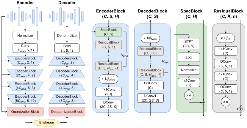
Figure 1: HILCodec model architecture. Conv(C, K, S), DConv(C, K, S), and DConvT(C, K, S) represent a convolution, a depthwise convolution, and a depthwise transposed convolution respectively, each with output channels of C, a kernel size of K, and a stride of S. 1x1Conv(C) denotes a pointwise convolution with output channels of C.

III-A Model Architecture

HILCodec is an end-to-end neural audio codec that leverages the time-domain fully convolutional Wave-U-Net. Following [38], HilCodec is composed of an encoder, a residual vector quantizer (RVQ), and a decoder. Given a raw waveform input, the encoder generates a feature vector for every 320 samples. The decoder reconstructs the waveform from a sequence of quantized features. The overall model architecture is illustrated in Fig. 1.

III-A1 Encoder-Decoder

Similar to [17], the encoder is composed of a convolution layer with $C_{enc}$ output channels followed by 4 convolution blocks and a quantization block. Each encoder block contains a spectrogram block (see Section III-A4) and $N_{enc}-1$ residual blocks, followed by a strided convolution for downsampling. The strides are set to 2, 4, 5, and 8. The quantization block is composed of a convolution layer with $D$ output channels, an $L_{2}$-normalization layer (see Section III-A3), and an RVQ with codebook vectors of $D$ dimensions.

The decoder mirrors the encoder’s structure, replacing strided convolutions with transposed convolutions for upsampling, and substituting the quantization block with a dequantization block. Each decoder block contains $N_{dec}$ residual blocks. The final convolution layer has $C_{dec}$ input channels. An ELU activation function [50] is inserted before every convolution layer, except the first one of the encoder. A hyperbolic tangent activation is inserted after the last convolution layer of the decoder to ensure that the final output waveform lies within the range of $-1$ and $1$.

In the domain of neural image compression, the prevalent approach involves the use of a compact encoder coupled with a larger decoder [59, 60]. Various neural audio codecs also adopted this paradigm [40, 42]. It is reported that downsizing the encoder has a minimal effect on performance, while a reduction in the decoder size significantly degrades audio quality [38]. The architecture of HILCodec is designed in accordance with these approaches. The encoder is configured with $C_{enc}$ set to 64 and the number of residual blocks $N_{enc}-1$ set to $2$, while the decoder is set up with $C_{dec}=96$ and $N_{dec}=3$.

To ensure streamability, all convolution layers are causal. They are designed as depthwise separable convolutions [51] which help to maintain performance while reducing computation. Additionally, we apply weight normalization [52] to further enhance the model’s performance.

III-A2 Residual Vector Quantizer

We employ the same training mechanism for the RVQ as in [38]. The codebook vectors in the RVQ are initialized using k-means clustering. As proposed in [55], when the encoder’s output $O_{e}$ is quantized to $O_{q}$ by the RVQ, the gradient $\nabla_{O_{q}}L$ is passed directly to $O_{e}$ during backpropagation. To ensure proximity between $O_{e}$ and $O_{q}$, a mean squared error loss between $O_{e}$ and $O_{q}$ is enforced on the encoder. The codebook vectors are updated using an exponential moving average (ema) with a smoothing factor of $0.99$. To prevent some codebook vectors from being unused, we reinitialize codebook vectors whose ema of usage per mini-batch falls below $0.5$.

III-A3 $L_{2}$-normalization

Since the advent of VQVAE [55], there has been a continous exploration for superior vector quantization. One such method is the $L_{2}$-normalization of the encoder outputs and codebook vectors, which has been proven to improve the codebook utilization and the final output quality of a generative model [56, 42]. Our experiments also corroborate its beneficial impact on audio quality (see Section VI-B). However, unlike [56] and [42], we do not directly apply $L_{2}$-normalization to the codebook vectors. As we employ RVQ, we naturally apply the $L_{2}$-normalization only to the encoder output before quantization. This method bolsters the training stability and enhances the audio quality of the model.

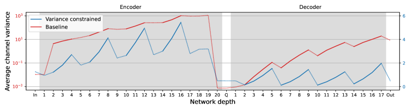
Figure 2: Comparison of the average channel variance according to network depth. On the x-axis, each number represents the network depth of the encoder and the decoder, and the terms “In”, “Q”, and “Out” denote the input waveform, the output of the residual vector quantizer, and the output waveform, respectively. The logaritmic y-scale on the left corresponds to the baseline model, while the linear y-scale on the right corresponds to the variance constrained model. The solid lines represent the residual blocks.

III-A4 Spectrogram Block

Traditional audio codecs exploit human-designed feature extractors for compression. In contrast, an end-to-end neural codec learns a feature extractor in a data-driven manner without requiring any expertise on audio coding. While a larger model can learn better features, it comes at the cost of increased computational complexity. To circumvent this, we extract additional features akin to those used in transform coding and feed them into the encoder network. Specifically, we insert a spectrogram block at the beginning of each encoder block. We provide a log spectrogram whose time resolution and frequency size match the time resolution and channel size of the encoder block’s input respectively. These multi-resolution spectrogram inputs assist the encoder with a limited parameter size in learning richer features. Importantly, we preserve the streaming nature of our model by using a causal STFT to obtain the spectrogram.

III-B Variance-Constrained Design

III-B1 Problems of Wave-U-Net

The Wave-U-Net architecture, which forms the backbone of the HilCodec generator, is a widely adopted model for end-to-end neural audio codecs [38, 39, 42, 41, 40]. However, we observed that the audio quality does not improve consistently as the depth of the model increases (see Fig. 5). This observation aligns with the results reported in [39], where the objective score for audio quality did not increase even after the number of residual blocks in encoder and decoder was tripled. To identify the reason, we concentrate on the signal propagation within the model’s forward pass.

Consider a tensor $\mathbf{x}$ with a shape of $B\times C\times T$ where $B$ denotes the batch size, $C$ denotes the channel size, and $T$ denotes time length. For simplicity, we define variance, or $\mathbf{Var}(\mathbf{x})$, as the average channel variance of $\mathbf{x}$, computed by taking the variance across the batch and time dimensions, and then averaging across the channel dimension:

$$\mathbf{Var}(\mathbf{x})\coloneqq\frac{1}{C}\sum_{c}\Bigg{[}\frac{1}{BT}\sum_{b}\sum_{t}\mathbf{x}^{2}_{b,c,t}\\ -\bigg{(}\frac{1}{BT}\sum_{b}\sum_{t}\mathbf{x}_{b,c,t}\bigg{)}^{2}\Bigg{]}.$$ (1)

Fig. 2 illustrates the signal propagation plot [62] of HILCodec right after initialization. Note that the y-axis of the baseline model is on a logarithmic scale ranging from $10^{-3}$ to $10^{3}$. In the encoder, the variance increases exponentially until it reaches the final layer, the $L_{2}$-normalization layer. In the decoder, the exponential growth of the variance persists until the end. The reasons and downsides for such a phenomenon can be well understood in the literature on deep normalized networks.

In the field of computer vision, the combination of BatchNorm [45] and skip connection [47] showed great performance gain and enabled very deep networks to be stably trained. Theoretical analyses have been conducted on the signal propagation of these networks to explain their success. Consider a network solely composed of residual blocks. The $n$-th residual block takes the form $\mathbf{x}_{n+1}=\mathbf{x}_{n}+f_{n}(\mathbf{x}_{n})$, where $\mathbf{x}_{n}$ is the input and $\mathbf{x}_{n+1}$ is the output. We refer to $f_{n}$ as the residual branch. Right after initialization, given that the input and the model weights are independent, $\mathbf{Var}(\mathbf{x}_{n+1})=\mathbf{Var}(\mathbf{x}_{n})+\mathbf{Var}(f_{n}(\mathbf{x}_{n}))$. Reference [61] showed that if $f_{n}$ is a network without any normalization layer, $\mathbf{Var}(f(\mathbf{x}_{n}))\approx\mathbf{Var}(\mathbf{x}_{n})$, leading to $\mathbf{Var}(\mathbf{x}_{n+1})\approx 2\mathbf{Var}(\mathbf{x}_{n})$. This implies that the variance increases exponentially according to the network depth $n$. On the other hand, if $f_{n}$ is a normalized network with appropriate initialization, $\mathbf{Var}(f_{n}(\mathbf{x}_{n}))\approx 1$, resulting in $\mathbf{Var}(\mathbf{x}_{n+1})\approx n+1$. This linear growth is beneficial to the model’s signal propagation $-$ it implies that the output of the residual branch $f_{n}(\mathbf{x}_{n})$ contributes only a $\frac{1}{n+1}$ fraction to $\mathbf{x}_{n+1}$. As a result, the output of each residual block is dominated by a skip connection, leading to stable training even for very deep networks. On the other hand, in un-normalized networks, both a residual branch and skip connection contribute equally to the output of each residual block, hindering signal propagation.

Since the Wave-U-Net architecture doesn’t contain any normalization layer, it experiences an exponential growth in variance as a function of network depth, resulting in performance degradation as illustrated in Fig. 5. Also, due to the high dynamic range of the baseline model’s signal propagation, mixed-precision training [54] fails when the number of residual blocks in each encoder/decoder block exceeds two. Prior works have indirectly addressed this issue by increasing the network’s width instead of its depth. For instance, HiFi-GAN employs multi-receptive field fusion modules, where the outputs from multiple parallel residual blocks are aggregated to yield the final output, instead of sequentially connecting each block. Furthermore, AudioDec extends this structure by explicitly broadening the network width using grouped convolutions.

Our goal is to directly solve the problem of exponential variance growth, rather than merely circumventing it. The most straightforward solution is to incorporate a normalization layer into every residual block. Nevertheless, our preliminary experiments with various normalization layers, including batch normalization and layer normalization layers [46], resulted in even poorer performance. We can only conjecture the reasons $-$ perhaps the batch size was insufficient due to hardware constraints, or the normalization layers we used were ill-suited for the waveform domain. To address this, instead of relying on normalization layers, we propose a variance-constrained design which facilitates proper signal propagation. This encompasses the residual block design, input and output normalization, and zero initialization of residual branches. As shown in Fig. 5, after applying our methods, the audio quality improves according to the network depth.

III-B2 Variance-Constrained Residual Block

In this subsection, we present the Variance-Constrained Residual Block (VCRB) designed to downscale the variance of the output of each residual branch such that the variance increases linearly with the network depth. It is motivated by the NFNet block [62] in image domain. A VCRB can be mathematically written as

$$\mathbf{x}_{n+1}=\mathbf{x}_{n}+\alpha\cdot f_{n}\bigg{(}\frac{\mathbf{x}_{n}}{\beta_{n}}\bigg{)},$$ (2)

where $\alpha$ and $\beta_{n}$ are fixed scalars to be discussed. We consider the residual branch $f_{n}$ right after initialization. Also, we assume that the network input $\mathbf{x}_{0}$ consists of i.i.d. random variables with a mean of $0$ and a standard deviation of $1$, and $f_{n}(\cdot)$ is a sample function of a random process indexed by $\mathbf{x}$. There are three key components in (2). Firstly, we randomly initialize the parameters of $f_{n}$ such that $\mathbf{Var}(f_{n}(\mathbf{x}_{n}))=\mathbf{Var}(\mathbf{x}_{n})$. More specifically, when a convolution layer follows an activation function, we apply He initialization [48]. When it doesn’t, we apply LeCun initialization [49] (see Appendix A). Secondly, we analytically calculate $\mathbf{Var}(\mathbf{x}_{n})$ (see (6)) and set

$$\beta_{n}=\sqrt{\mathbf{Var}(\mathbf{x}_{n})}.$$ (3)

This ensures that the variance of the input (and also the output) of $f_{n}(\cdot)$ is $1$:

$$\mathbf{Var}\Bigg{(}f_{n}\bigg{(}\frac{\mathbf{x}_{n}}{\beta_{n}}\bigg{)}\Bigg{)}=\mathbf{Var}\bigg{(}\frac{\mathbf{x}_{n}}{\beta_{n}}\bigg{)}=1.$$ (4)

Thirdly, we set

$$\alpha=\frac{1}{\sqrt{N}},$$ (5)

where $N$ is the number of residual blocks in an encoder or decoder block. Since $\mathbf{Var}(\mathbf{x}_{0})=1$, the variance of the output from the $n$-th residual block can be calculated as follows:

$$\begin{split}\mathbf{Var}(\mathbf{x}_{n})&=\mathbf{Var}(\mathbf{x}_{n-1})+\mathbf{Var}\Bigg{(}\alpha\cdot f_{n-1}\bigg{(}\frac{\mathbf{x}_{n-1}}{\beta_{n-1}}\bigg{)}\Bigg{)}\\ &=\mathbf{Var}(\mathbf{x}_{n-1})+\frac{1}{N}\\ &=\cdots\\ &=\mathbf{Var}(\mathbf{x}_{0})+\frac{n}{N}\\ &=1+\frac{n}{N}.\end{split}$$ (6)

(6) implies that the encoder/decoder blocks composed of VCRB possess the desired property of linear variance increment along the network depth.

III-B3 Other Building Blocks

For the spectrogram blocks described in Section III-A4, we treat them as a special type of residual block. This means that similar to the other residual blocks, we scale the output of each spectrogram block $g(\cdot)$ as:

$$\mathbf{y}=\mathbf{x}+\alpha\cdot g(\mathbf{s}),$$ (7)

where $\mathbf{s}$ is a spectrogram input. Assuming $\mathbf{s}$ has unit variance, (7) ensures $\mathbf{Var}(\mathbf{y})=1+1/N$.

As illustrated in Fig. 1, at the end of each encoder block, there exists a strided convolution for downsampling. Since it follows $N_{enc}$ sequential residual blocks, its input variance equals $2$ according to (6). Therefore, we divide its input by $\beta_{N_{enc}}=\sqrt{2}$. Similarly, we divide the output of each decoder block by $\beta_{N_{dec}}=\sqrt{2}$.

III-B4 Input/Output Normalization

We further normalize the input and output of both the encoder and decoder. We compute the mean and standard deviation of $10000$ randomly sampled audio chunks from the training dataset. At the beginning of the encoder, we insert a normalization layer using pre-calculated statistics. We also insert normalization layers for multi-resolution spectrogram inputs. In the decoder, right after the final convolution and prior to the hyperbolic tangent activation, we insert a de-normalization layer. The final element we normalize is the output of the encoder (equivalently the input of the decoder before quantization), denoted as $\mathbf{z}$. Since we apply $l_{2}$-normalization before quantization as discussed in Section III-A3, the mean square of $\mathbf{z}$ is $\mathbb{E}(\mathbf{z}^{2})=1/C$, where $C$ is the channel dimension of $\mathbf{z}$. Ignoring the square of the mean of $\mathbf{z}$, we multiply $\sqrt{C}$ to $\mathbf{z}$ after $l_{2}$-normalization so that the variance is approximately $1$ as given by

$$\mathbf{Var}(\sqrt{C}\cdot\mathbf{z})=C\cdot\mathbb{E}(\mathbf{z}^{2})-C\cdot\mathbb{E}(\mathbf{z})^{2}\approx C\cdot\mathbb{E}(\mathbf{z}^{2})=1.$$ (8)

After applying variance-constrained blocks and input/output normalization, the variance of the network right after initialization remains in a reasonable dynamic range as illustrated in Fig. 2.

III-B5 Zero-Initialized Residual Branch

For deep residual networks, it has been empirically shown that initializing every residual block to be an identity function at the beginning of training can further enhance the performance [53]. Following [62], we add a scalar parameter initialized to zero at the end of each residual branch, which we also found beneficial for the fast convergence of the model. While this zero-initialization scheme results in a modification of $\beta_{n}$ in Section III-B2, we found that ignoring this effect does not detrimentally impact the performance of our model.

IV Discriminator

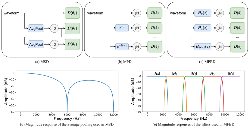
Figure 3: (a)-(c): Comparison of different discriminators. (d)-(e): Magnitude responses of filters they use. (a) AvgPool denotes an average pooling. (b) $z^{-n}$ denotes $n$-sample delay. (a)-(c) $\downarrow$$N$ denotes downsampling by a factor of $N$, and $D(\theta)$ denotes a sub-discriminator with a parameter $\theta$. MSD uses distinct sub-discriminators for different hierarchies while MPD and MFBD use shared parameters across the sub-bands.

We apply two types of discriminators: a novel aliasing-free waveform domain discriminator and a widely used time-frequency domain discriminator.

IV-A Multi-Filter Bank Discriminator

IV-A1 Problems of previous discriminators

It is well-known that audio encompasses a significantly large number of samples within a short time span. For instance, an audio clip that is 3 seconds long at a sampling rate of 24kHz contains 72,000 samples. Consequently, waveform domain discriminators typically accept audio inputs after downsampling. As shown in Fig. 3(a) and (b), the Multi-Scale Discriminator (MSD) [22] uses average pooling, and the Multi-Period Discriminator (MPD) [24] relies on a plain downsampling. The combination of MSD and MPD has achieved significant success in the field of neural vocoders and has been employed in various neural audio codecs [41, 40, 42]. However, from a signal processing perspective, these discriminators induce distortion to the input signal. MPD relies on a plain downsampling, which causes aliasing of the signal. In the case of MSD, average pooling can be interpreted as a low-pass filter using a rectangular window. Fig. 3(d) depicts the magnitude response of a 4-tap average pooling used in MSD. The passband is not flat, the transition band is too wide and not steep, and the attenuation level in the stopband is too low. It is evident that average pooling distorts input signal and is insufficient to prevent aliasing caused by subsequent downsampling. Furthermore, after average pooling, MSD is limited to modeling low-frequency components only. This highlights the need for a more sophisticated waveform-domain discriminator capable of preventing distortion and modeling the entire frequency spectrum.

IV-A2 Proposed discriminator

We propose a novel Multi-Filter Bank Discriminator (MFBD). As illustrated in Fig. 3(c), it initially transforms the waveform into $N$ sub-bands using a filter bank, followed by a downsampling with a factor of $N$. Each sub-band is then fed into a single discriminator with shared weights. This enables the discriminator to observe the entire frequency components with minimum distortion. Similar to [24], MFBD is composed of multiple sub-discriminators with the number of sub-bands $N\in\{1,2,3,5,7,11\}$. This approach has two beneficial effects. Sub-discriminators with small $N$ can model short-term dependencies, while those with large $N$ can model long-term dependencies. Additionally, because we use a coprime number of sub-bands, even the distortion in transition bands can be covered by other sub-discriminators. The model architecture of MFBD is configured in the same way as MPD.

Similar approach was also introduced in Avocodo [27]. It uses pseudo-quadratic mirror filter bank [7] to obtain sub-band features and feed the entire features to a discriminator. The key differences are that ours have more generalization ability by using a shared discriminator across different sub-bands. We also utilize multiple sub-discriminators with co-prime number of sub-bands to cope with distortion in transition bands. Our experiments demonstrate the superiority of MFBD over discriminators of Avocodo (see Section VI-B). For more detailed comparison, please refer to Appendix B.

IV-B Multi-Resolution Spectrogram Discriminator

Along with MFBD, we also apply the multi-resolution spectrogram discriminator (MRSD). Simultaneously using both waveform domain discriminator and time-frequency domain discriminator has been proven to enhance the audio quality [38, 40]. We obtain complex spectrograms with Fourier transform sizes of $\{128,256,512,1024\}$ and hop lengths of $\{32,64,128,256\}$. We represent each spectrogram as a real-valued tensor with two channels (real and imaginary) and pass it through a discriminator composed of 2D convolutions.

V Experimental Setup

V-A Training Objective

Let $\mathcal{G}$ denote a generator composed of an encoder $\mathcal{G}_{e}$, a quantizer $\mathcal{Q}$, and a decoder $\mathcal{G}_{d}$. Let $\mathcal{D}_{1}$ denote MFBD, $\mathcal{D}_{2}$ denote MRSD, $x$ denote the input waveform and $\hat{x}=\mathcal{G}(x)$ denote the waveform reconstructed by the generator.

V-A1 Reconstruction Loss

To reduce the distortion in $\hat{x}$, we employ a reconstruction loss. It comprises the mean absolute errors and mean squared errors between multi-resolution log mel spectrograms of $x$ and $\hat{x}$ as given by

$$\mathcal{L}_{rec}=\sum_{i\in\{1,\cdots,6\}}\|\mathcal{S}_{i}(x)-\mathcal{S}_{i}(\hat{x})\|_{1}+\|\mathcal{S}_{i}(x)-\mathcal{S}_{i}(\hat{x})\|_{2}^{2},$$ (9)

where $\|\cdot\|_{1}$ represents a mean of absolute values of elements in a given tensor, $\|\cdot\|_{2}^{2}$ represents a mean of squared values, and $\mathcal{S}_{i}$ represents a log mel spectrogram computed with the Fourier transform size of $2^{i+4}$, hop length of $2^{i+2}$ and the number of mel filters set to the $i$-th element of the set {6, 12, 23, 45, 88, 128}. The number of mel filters is determined such that every mel filter has at least one non-zero value [42].

V-A2 GAN Loss

We adopt the GAN loss in [39] where the generator loss is defined as

$$\mathcal{L}_{g}=\sum_{j}\mathbb{E}\Big{[}\max\big{(}0,1-\mathcal{D}_{j}(\hat{x})\big{)}\Big{]},$$ (10)

and the discriminator loss is defined as

$$\mathcal{L}_{d}=\sum_{j}\mathbb{E}\left[\max\big{(}0,1-\mathcal{D}_{j}(x)\big{)}+\max\big{(}0,1+\mathcal{D}_{j}(\hat{x})\big{)}\right].$$ (11)

V-A3 Feature Matching Loss

We use the normalized feature matching loss [39] as

$$\mathcal{L}_{fm}=\sum_{j}\sum_{l}\Bigg{[}\frac{\|\mathcal{D}_{j}^{l}(x)-\mathcal{D}^{l}_{j}(\hat{x})\|_{1}}{\|\mathcal{D}_{j}^{l}(x)\|_{1}}\Bigg{]},$$ (12)

where $\mathcal{D}_{j}^{l}$ is the $l$-th layer of the $j$-th discriminator

V-A4 Commitment Loss

To further reduce the quantization noise, we impose the commitment loss [55] to the encoder $\mathcal{G}_{e}$ as given by

$$\mathcal{L}_{c}=\left\|\mathcal{G}_{e}(x)-\mathcal{Q}\Big{(}\text{sg}[\mathcal{G}_{e}(x)]\Big{)}\right\|_{2}^{2},$$ (13)

where sg[$\cdot$] stands for the stop-gradient operator. Since the codebooks in the residual vector quantizer are updated using an exponential moving average of $\mathcal{G}_{e}(x)$, we do not give explicit loss to the codebooks.

V-A5 Loss Balancer

While the training objective for discriminators is solely composed of $\mathcal{L}_{d}$, the training objective for the generator is a combination of $\mathcal{L}_{g}$, $\mathcal{L}_{fm}$, $\mathcal{L}_{rec}$ and $\mathcal{L}_{c}$. Naturally, this requires an extensive hyperparameter search to find an optimal coefficient for each loss term. To address this issue, we adopted a loss balancer introduced in [39] because of its robustness to loss coefficients and ability to stabilize training. Without a loss balancer, $\mathcal{G}$ is trained with a loss

$$\mathcal{L}=\lambda_{rec}\cdot\mathcal{L}_{rec}+\lambda_{g}\cdot\mathcal{L}_{g}+\lambda_{fm}\cdot\mathcal{L}_{fm}=\sum_{i}\lambda_{i}\cdot\mathcal{L}_{i},$$ (14)

where we temporarily exclude $\mathcal{L}_{c}$. Then the parameter $w$ of the generator is updated using

$$\begin{split}\nabla_{w}&:=\frac{\partial\mathcal{L}}{\partial w}=\frac{\partial\mathcal{L}}{\partial\hat{x}}\frac{\partial\hat{x}}{\partial w}=\left(\sum_{i}\lambda_{i}\cdot\frac{\partial\mathcal{L}_{i}}{\partial\hat{x}}\right)\frac{\partial\hat{x}}{\partial w}\\ &=\left(\sum_{i}\lambda_{i}\cdot g_{i}\right)\frac{\partial\hat{x}}{\partial w},\end{split}$$ (15)

where $g_{i}:=\partial\mathcal{L}_{i}/\partial\hat{x}$. The loss balancer aims to remove the effect of the size of gradient $\|g_{i}\|_{2}$ and retain only the direction $g_{i}/\|g_{i}\|_{2}$ so that $\lambda_{i}$ becomes the true scale of each loss $\mathcal{L}_{i}$. Using the loss balancer, $w$ is updated using

$$\widetilde{\nabla}_{w}=\left(\sum_{i}\lambda_{i}\cdot\frac{g_{i}}{\mathbb{E}\left[\|g_{i}\|_{2}\right]}\right)\frac{\partial\hat{x}}{\partial w}+\lambda_{c}\cdot\frac{\partial\mathcal{L}_{c}}{\partial w},$$ (16)

where $\mathbb{E}[\cdot]$ is an exponential moving average. Since we cannot calculate the gradient of $\hat{x}$ with respect to $\mathcal{L}_{c}$, we did not apply the loss balancer to $\mathcal{L}_{c}$.

V-B Datasets and Training Settings

We trained two versions of HILCodec: one trained on clean speech, and the other trained on general audio, including clean speech, noisy speech and music. For clean speech datasets, we used speech segments from DNS Challenge 4 [63] and the VCTK-0.92 corpus [64]. For noisy speech, we mixed clean speech segments with noise segments from DNS Challenge 4 during training on-the-fly. For music, we used Jamendo [65]. All audio files were downsampled to a sampling rate of 24kHz. During training on general audio, we sampled each type of audio with the same probability. We randomly extracted 1 second long segment from each audio file, applied a random gain in [-10dB, 6dB], and scaled down the audio when a clipping occurred during a mixing or a random gain adjustment.

For GAN training, we adopted simultaneous GAN [44]. Each model was trained for 468k iterations using 2 RTX 3090 GPUs with a batch size of 24 per GPU, which took 114 hours. We used the AdamP optimizer [57] with an initial learning rate of $5\cdot 10^{-4}$ and a weight decay of $10^{-5}$. We utilized a cosine annealing learning rate scheduler [58] with a linear warmup for 5k iterations.

V-C Baselines

We compare HILCodec to various end-to-end neural audio codecs that are publicly available. EnCodec [39] and Descript Audio Codec [42] are models trained on general audio. HiFi-Codec [41] and AudioDec [40] are models trained on clean speech. For all models, we used versions with the same sampling rate of 24kHz. We also included EVS [9], the signal processing-based audio codec which has demonstrated state-of-the-art performance among traditional codecs [10]. It is a hybrid codec that uses LPC when compressing speech and uses transform coding when compressing the others. Since it does not support the sampling rate of 24kHz, we upsampled the audio to 32kHz, compressed with EVS, and downsampled back to 24kHz.

V-D Evaluation Metrics

V-D1 Subjective Metric

To compare HILCodec with the baselines, we conducted MUSHRA test [66] using webMUSHRA framework [68]. As reference audios, we selected four clean speeches, four noisy speeches, and four music pieces for general audio coding, and 12 clean speeches for speech coding. For each test item, we included a low anchor, which was a low-pass filtered version of the reference audio with a cut-off frequency of 3.5kHz, but excluded a mid anchor with a cut-off frequency of 7kHz. Post-screening was performed to exclude assessors who rated hidden references lower than a score of 90 more than 15% of the test items or rated low anchors higher than 90 more than 15% of the test items. The number of assessors after post-screening was 11.

V-D2 Objective Metric

For model developments and ablation studies, we utilized ViSQOL Audio v3 [67]. We selected 100 audio samples for each of three categories, upsampled reference audios and coded audios to a sampling rate of 48kHz, and calculated ViSQOL scores.

VI Results

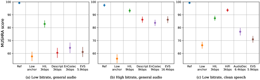
Figure 4: MUSHRA scores of various codecs with 95% confidence intervals. (a) Low bitrate, trained and evaluated on general audio. (b) High bitrate, trained and evaluated on general audio. (c) Low bitrate, trained and evaluated on clean speech.

VI-A Subjective Quality Comparison

Fig. 4 illustrates the MUSHRA scores obtained from HILCodec and the other baseline codecs. Note that HILCodec, EnCodec, AudioDec, and EVS are streamable while Descript and HiFi-Codec are not. Also, HILCodec has a complexity smaller than most of the other neural codecs (see Section VI-C). In Fig. 4(a), we can see that for general audio coding, HILCodec at 3kbps significantly outperforms Descript at 3kbps, EnCodec at 3kbps, and EVS at 5.9kbps. Moreover, in Fig. 4(b), HILCodec at 9kbps surpasses other neural audio codecs at 9kbps and EVS at 16.4kbps. In Fig. 4(c), for clean speech coding, HILCodec at 3kbps has slightly lower sound quality than high-complexity unstreamable HiFi-Codec at 3kbps. However, it outperforms AudioDec at 6.4kbps and EVS at 5.9kbps by significant margins.

VI-B Ablation Studies

TABLE I: Ablation studies for the generator. Mean and 95% confidence interval values are reported.

Ablation	ViSQOL
HILCodec	4.105 $\pm$ 0.024
Architecture
No $L_{2}$-normalization	3.904 $\pm$ 0.025
No spectrogram blocks	4.081 $\pm$ 0.026
Variance-Constrained Design
Plain residual blocks	4.082 $\pm$ 0.026
No input/output normalization	4.059 $\pm$ 0.024
No zero initialization	4.092 $\pm$ 0.023

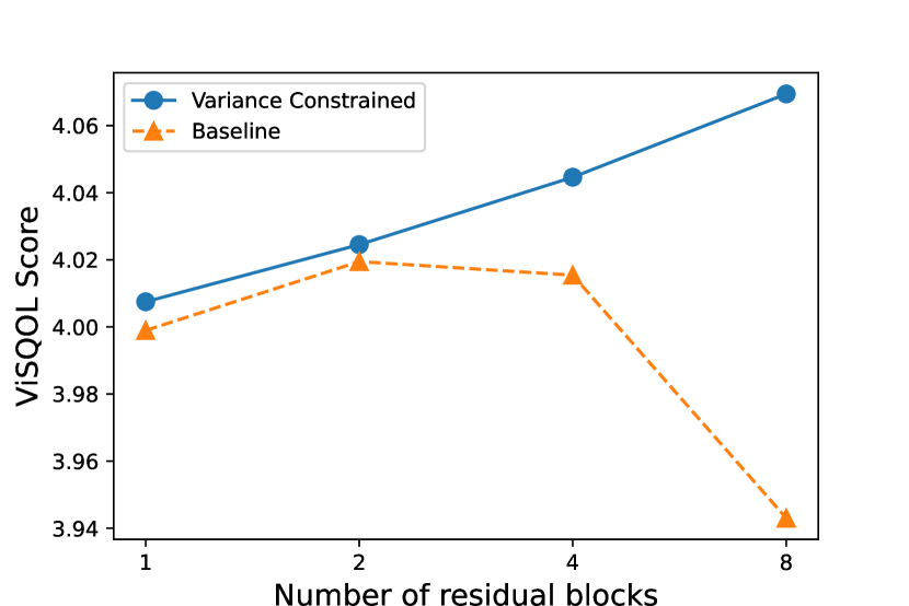
Figure 5: ViSQOL scores according to the number of residual blocks in each encoder and decoder block. We train each model three times with different seeds and plot the mean value.

We performed ablation studies to prove the effectiveness of the proposed techniques. Because of training resource limits, all models presented in this subsection were trained with a smaller timestep of 156k iterations.

VI-B1 Generator

Starting from HILCodec trained on general audio, we removed each generator component while maintaining the other components and measured ViSQOL scores. The results are presented in Table I. Regarding the architectural choice, removing $L_{2}$-normalization and spectrogram blocks each results in quality degradation. Moreover, replacing the variance-constrained residual blocks with plain residual blocks, removing input/output normalization, and removing zero initialization each results in a lower ViSQOL score. This indicates that each component we propose has a beneficial effect on the audio quality.

To further analyze the impact of variance-constrained design, we performed additional experiments as follows. We built a smaller version of HILCodec with $C_{enc}=32$ and $C_{dec}=32$, which we call the variance-constrained model. We also built a baseline model that was exactly the same as the variance-constrained model, except that it did not follow the proposed variance-constrained design: it consisted of plain residual blocks, discarded input/output normalization, and did not employ zero initialization. We tracked the ViSQOL scores at 3kbps while varying the number of residual blocks in each encoder and decoder block from 1 to 8. We trained each model with three different seeds and computed the mean values. In Fig. 5, the objective quality of the baseline model starts to degrade after the number of residual blocks becomes four. On the other hand, the variance-constrained model shows steadily increasing ViSQOL scores along the network depth. This demonstrates the validity of the variance-constrained design.

VI-B2 Discriminator

TABLE II: MUSHRA scores of different discriminators. Mean and 95% confidence interval values are reported.

Discriminators	MUSHRA
MPD+MSD (HiFi-GAN)	69.32 $\pm$ 2.95
CoMBD+SBD (Avocodo)	74.66 $\pm$ 3.34
MFBD+MRSD (HILCodec)	82.43 $\pm$ 2.27

We compared the subjective quality of the proposed discriminators with that of MPD and MSD used in HiFi-GAN, and CoMBD and SBD used in Avocodo. For MPD and MSD, we used the same generator and training configurations to ensure a fair comparison. However, since CoMBD operates on multiple resolutions, we modified the generator so that the last three decoder blocks generate waveforms with different sampling rates, as in Avocodo. This made it impossible to use the loss balancer. Instead, we strictly followed the loss functions and loss coefficients used in [27]. Table II shows the MUSHRA scores for different combinations of discriminators. MFBD and MRSD provide better perceptual quality than the other discriminators.

VI-C Computational Complexity

TABLE III: Complexity of various neural audio codecs.

Model	#Params (M)	MAC (G)		RTF
		Enc	Dec	Enc	Dec
HILCodec	9.58	3.29	7.46	2.47	1.13
EnCodec	14.85	1.65	1.49	4.22	4.25
AudioDec	23.27	3.35	23.89	2.96	0.94
Descript	74.18	3.41	30.23	-
HiFi-Codec	63.63	20.86	21.15	-

We compared HILCodec against other neural audio codecs in terms of computational complexity. We measured the number of parameters, multiply-add counts (MAC) for coding one second long input waveform, and real-time factor (RTF). RTF is defined as the ratio of the length of the input waveform to the time consumed for coding. An RTF higher than 1 means the codec operates in real-time. When calculating RTF, we used one thread of a server CPU (Intel Xeon 6248R 3GHz), exported each model to ONNX Runtime [69], and simulated a streaming condition. Namely, for HILCodec and EnCodec, a chunk with 320 waveform samples was encoded and decoded at a time, and for AudioDec, a chunk with 300 samples was processed at a time. For every convolution layer with a kernel size larger than one, previous samples were stored in a cache and used to calculate the current chunk. Descript and HiFi-Codec are not streamable, so their RTFs are not reported. The results are shown in Table III. HILCodec has the smallest number of parameters, requiring minimum memory to store and load model parameters. Moreover, the MAC of HILCodec is smaller than AudioDec, Descript, and HiFi-Codec, and its RTF is higher than 1.

VII Conclusion

We have addressed the issues of previous neural audio codecs: huge complexity, exponential variance growth of the generator, and distortions induced by the discriminator. As a solution, we have proposed a lightweight backbone architecture, a variance-constrained design, and a distortion-free discriminator using multiple filter banks. Combining these elements, the proposed codec, HILCodec, achieves superior quality compared to other deep learning-based and signal processing-based audio codecs across various bitrates and audio types. Although we concentrate on building a real-time streaming codec in this work, we expect that our findings can be applied to construct larger and more powerful models.

Appendix A Variance of Residual Branches

In Section III-B2, we construct the VCRB such that the variance after initialization follows (6). However, in Fig. 2, although the variance increases linearly with the network depth, it does not strictly follow (6). It is demonstrated that for exactness, we must use scaled weight standardization (Scaled WS) [62]. However, in our early experiments, using Scaled WS resulted in a slightly worse ViSQOL score. Reference [62] also experienced similar degradation and hypothesized that Scaled WS harms the performance of depthwise convolutions. Therefore, as an alternative, we carefully apply initialization for each layer. For layers where an activation function does not come immediately after, we apply LeCun initialization so that $\mathbf{Var}(W\mathbf{x})\approx\mathbf{Var}(\mathbf{x})$ where $W$ is a weight parameter. For layers with subsequent activation functions, we apply He initialization so that $\mathbf{Var}(\sigma(W\mathbf{x})))\approx\mathbf{Var}(\mathbf{x})$. Through these methods, despite the model do not exactly follow (6), it achieves a linear variance increment.

Appendix B Differences Between MFBD and MSD

We present detailed comparisons between SBD used in Avocodo and MFBD used in HILCodec. First, SBD decomposes the input signal into 16 sub-bands while MFBD uses co-prime numbers of sub-bands $N\in\{1,2,3,5,7,11\}$. As described in Section IV-A2, this enables MFBD to model both long- and short-term dependencies and handle distortions in transition bands. Second, in SBD, a single sub-discriminator accepts the entire 16 sub-bands simultaneously using a convolution layer with input channels 16. On the other hand, in MFBD, a sub-discriminator accepts each sub-band separately using a convolution layer with input channels of 1. However, the parameter of the sub-discriminator is shared across sub-bands as illustrated in Fig. 3(c). Third, in SBD, there exists a sub-discriminator that operates on a transposed sub-band feature. This means that the number of sub-bands becomes the length of the input, and the length of the sub-band feature becomes the channel size of the input. In MFBD, we do not employ such a sub-discriminator. We suspect these overall differences result in the superior performance of MFBD over SBD.

References

References

- [1] H. Dudley, “Remaking speech,” in J. Acoust. Soc. Amer., vol. 11, pp. 169-177, 1939.
- [2] J. Makhoul, “Linear prediction: A tutorial review,” Proc. IEEE, vol. 63, no. 4, pp. 561–580, Apr. 1975.
- [3] B. Atal and M. R. Schroeder, “Adaptive predictive coding of speech signals,” in Conf. Comm. and Proc., pp. 360-361, 1967.
- [4] V. K. Goyal, “Theoretical foundations of transform coding,” IEEE Signal Process. Mag., vol. 18, no. 5, pp. 9-21, Sept. 2001.
- [5] R. Gray, “Vector quantization,” IEEE Assp Mag., vol. 1, no. 2, pp. 4–29, Apr. 1984.
- [6] A. Vasuki and P. Vanathi, “A review of vector quantization techniques,” IEEE Potentials, vol. 25, no. 4, pp. 39–47, Jul./Aug. 2006.
- [7] T. Q. Nguyen, “Near-perfect-reconstruction pseudo-QMF banks,” in IEEE Trans. Signal Process., vol. 42, no. 1, pp. 65-76, Jan. 1994.
- [8] J. Makinen, B. Bessette, S. Bruhn, P. Ojala, R. Salami and A. Taleb, “AMR-WB+: a new audio coding standard for 3rd generation mobile audio services,” in Proc. IEEE Int. Conf. Acoust., Speech, Signal Process., Philadelphia, PA, USA, 2005, vol. 2, pp. ii/1109-ii/1112.
- [9] M. Dietz et al., “Overview of the EVS codec architecture,” in Proc. IEEE Int. Conf. Acoust., Speech, Signal Process., South Brisbane, QLD, Australia, 2015, pp. 5698–5702.
- [10] A. Rämö and H. Toukomaa, “Subjective quality evaluation of the 3GPP EVS codec,” in Proc. IEEE Int. Conf. Acoust., Speech, Signal Process., South Brisbane, QLD, Australia, 2015, pp. 5157-5161.
- [11] M. Neuendorf, P. Gournay, M. Multrus, J. Lecomte, B. Bessette, R. Geiger, S. Bayer, G. Fuchs, J. Hilpert, N. Rettelbach, R. Salami, G. Schuller, R. Lefebvre, and B. Grill, “Unified speech and audio coding scheme for high quality at low bitrates,” in Proc. IEEE Int. Conf. Acoust., Speech, Signal Process., Taipei, Taiwan, 2009, pp. 1-4.
- [12] T. Painter and A. Spanias, “Perceptual coding of digital audio,” Proc. IEEE, vol. 88, no.4, pp. 451-515, Apr. 2000.
- [13] K. Brandenburg and G. Stoll, “ISO/MPEG-1 Audio: A Genereic Standard for Coding of High Quality Digital Audio,” J. Audio Eng. Soc., vol. 40, no. 10, pp. 780-792, Oct. 1994
- [14] M. Bosi, K. Brandenburg, S. Quackenbush, L. Fielder, K. Akagiri, H. Fuchs, M. Dietz, “ISO/IEC MPEG-2 Advanced Audio Coding,” J. Audio Eng. Soc., vol. 45, no. 10, pp. 789-814, Oct. 1997.
- [15] W. Dobson, J. Yang, K. Smart and F. Guo, “High Quality Low Complexity Scalable Wavelet Audio Coding,” in Proc. IEEE Int. Conf. Acoust., Speech, Signal Process., Munich, Germany, 1997.
- [16] D. Stoller, S. Ewert, and S. Dixon, “Wave-U-Net: a multi-scale neural network for end-to-end Audio Source Separation,” in Proc. IEEE Int. Conf. Acoust., Speech, Signal Process., Calgary, AB, Canada, 2018, pp. 131–135.
- [17] Y. Li, M. Tagliasacchi, O. Rybakov, V. Ungureanu, and D. Roblek, “Real-time speech frequency bandwidth extension,” in Proc. IEEE Int. Conf. Acoust., Speech, Signal Process., Toronto, ON, Canada, 2021, pp. 691–695.
- [18] A. van den Oord, S. Dieleman, H. Zen, K. Simonyan, O. Vinyals, A. Graves, N. Kalchbrenner, A. Senior, and K. Kavukcuoglu, “WaveNet: a generative model for raw audio,” 2016, arXiv:1609.03499.
- [19] N. Kalchbrenner, E. Elsen, K. Simonyan, S. Noury, N. Casagrande, E. Lockhart, F. Stimberg, A. van den Oord, S. Dieleman, and K. Kavukcuoglu, “Efficient neural audio synthesis,” in Proc. Int. Conf. Mach. Learn., Stockholm, Sweden, 2018, pp. 2410-2419.
- [20] A. van den Oord et al., “Parallel WaveNet: Fast high-fidelity speech synthesis,” in Proc. Int. Conf. Mach. Learn., Stockholm, Sweden, 2018, pp. 3918-3926.
- [21] R. Prenger, R. Valle, and B. Catanzaro, “Waveglow: A flow-based generative network for speech synthesis,” in Proc. IEEE Int. Conf. Acoust., Speech, Signal Process., Brighton, UK, 2019, pp. 3617-3621.
- [22] K. Kumar, R. Kumar, T. d. Boissiere, L. Gestin, W. Z. Teoh, J. Sotelo, A. d. Brebisson, Y. Bengio, and A. Courville, “MelGAN: Generative adversarial networks for conditional waveform synthesis,” in Proc. Adv. Neural Inf. Process. Syst., Vancouver, BC, Canada, Dec. 2019.
- [23] R. Yamamoto, E. Song, and J. -M. Kim, “Parallel Wavegan: A fast waveform generation model based on generative adversarial networks with multi-resolution spectrogram,” in Proc. IEEE Int. Conf. Acoust., Speech, Signal Process., Barcelona, Spain, 2020, pp. 6199-6203.
- [24] J. Kong, J. Kim, and J. Bae, “HiFi-GAN: Generative adversarial networks for efficient and high fidelity speech synthesis,” in Proc. Adv. neural Inf. Process. Syst., Vancouver, BC, Canada, 2020.
- [25] Z. Kong, W. Ping, J. Huang, K. Zhao, and B. Catanzaro, “DiffWave: A versatile diffusion model for audio synthesis,” in Proc. Int. Conf. Learn. Represent., Vienna, Austria, 2019.
- [26] N. Chen, Y. Zhang, H. Zen, R. J. Weiss, M. Norouzi, and W. Chan, “WaveGrad: Estimating gradients for waveform generation,” in Proc. Int. Conf. Learn. Represent., Vienna, Austria, 2019.
- [27] T. Bak, J. Lee, H. Bae, J. Yang, J.-S. Bae, and Y.-S. Joo, “Avocodo: Generative adversarial network for artifact-free vocoder,” in Proc. AAAI Conf. Artif. Intell., vol. 37, no. 11, pp. 12562-12570, 2023.
- [28] W. Jang, D. Lim, J. Yoon, B. Kim, and J. Kim, “UnivNet, A neural vocoder with multi-resolution spectrogram discriminators for high-fidelity waveform generation,” in Proc. Interspeech, Brno, Czechia, 2021.
- [29] S.-g. Lee, W. Ping, B. Ginsburg, B. Catanzaro, and S. Yoon, “BigVGAN: A universal neural vocoder with large-scale training,” in Proc. Int. Conf. Learn. Represent., Kigali, Rwanda, 2023.
- [30] A. Biswas and D. Jia, “Audio codec enhancement with generative adversarial networks,” in Proc. IEEE Int. Conf. Acoust., Speech, Signal Process., Barcelona, Spain, 2020, pp. 356–360.
- [31] S. Korse, N. Pia, K. Gupta, and G. Fuchs, “PostGAN: A GAN-Based Post-Processor to Enhance the Quality of Coded Speech,” in Proc. IEEE Int. Conf. Acoust., Speech, Signal Process., Singapore, Singapore, 2022, pp. 831-835.
- [32] J. Lin, K. Kalgaonkar, Q. He and X. Lei, “Speech Enhancement for Low Bit Rate Speech Codec,” in Proc. IEEE Int. Conf. Acoust., Speech, Signal Process., Singapore, Singapore, 2022, pp. 831-835.
- [33] J. -M. Valin and J. Skoglund, “LPCNET: Improving Neural Speech Synthesis through Linear Prediction,” in Proc. IEEE Int. Conf. Acoust., Speech, Signal Process., Brighton, UK, 2019, pp. 5891-589.
- [34] H. Y. Kim, J. W. Yoon, W. I. Cho, and N. S. Kim, “Neurally Optimized Decoder for Low Bitrate Speech Codec,” in IEEE Signal Process. Lett., vol. 29, pp. 244-248, 2022
- [35] W. B. Kleijn, F. S. C. Lim, A. Luebs, J. Skoglund, F. Stimberg, Q. Wang, and T. C. Walters, “WaveNet based low rate speech coding,” in Proc. IEEE Int. Conf. Acoust., Speech, Signal Process., Calgary, AB, Canada, 2018, pp. 676-680. IEEE Int. Conf. Acoust., Speech, Signal Process., 2018, pp. 676–680.
- [36] S. Morishima, H. Harashima and Y. Katayama, “Speech coding based on a multi-layer neural network,” in Proc. IEEE Int. Conf. Commun., Including Supercomm Tech. Sessions, Atlanta, GA, USA, 1990, pp. 429-433, vol. 2.
- [37] S. Kankanahalli, “End-to-end optimized speech coding with deep neural networks,” in Proc. IEEE Int. Conf. Acoust., Speech, Signal Process., 2018, pp. 2521–2525.
- [38] N. Zeghidour, A. Luebs, A. Omran, J. Skoglund and M. Tagliasacchi, “Soundstream: An end-to-end neural audio codec,” IEEE/ACM Trans. Audio, Speech, Lang. Process., vol. 30, pp. 495-507, 2022.
- [39] A. Défossez, J. Copet, G. Synnaeve, and Y. Adi, “High Fidelity Neural Audio Compression,” Trans. Mach. Learn. Res., Sep. 2023.
- [40] Y. -C. Wu, I. D. Gebru, D. Marković and A. Richard, “Audiodec: An Open-Source Streaming High-Fidelity Neural Audio Codec,” in Proc. IEEE Int. Conf. Acoust., Speech, Signal Process., Rhodes Island, Greece, 2023, pp. 1-5.
- [41] D. Yang, S. Liu, R. Huang, J. Tian, C. Weng, and Y. Zou, “HiFi-Codec: Group-residual vector quantization for high fidelity audio codec,” 2023, arXiv:2305.02765.
- [42] R. Kumar, P. Seetharaman, A. Luebs, I. Kumar, and K. Kumar, “High-fidelity audio compression with improved RVQGAN,” in Proc. Adv. Neural Inf. Process. Syst., New Orleans, LA, USA, 2023.
- [43] I. Goodfellow, J. Pouget-Abadie, M. Mirza, B. Xu, D. Warde-Farley, S. Ozair, A. Courville, and Y. Bengio, “Generative adversarial nets,” in Proc. Adv. Neural Inf. Process. Syst., Montreal, Canada, 2014.
- [44] V. Nagarajan and J. Z. Kolter, “Gradient descent GAN optimization is locally stable,” in Proc. Adv. Neural Inf. Process. Syst., Long Beach, CA, USA, 2017.
- [45] S. Ioffe and C. Szegedy, “Batch normalization: accelerating deep network training by reducing internal covariate shift,” in Proc. Int. Conf. Mach. Learn., Lille, France, 2015, pp. 448-456.
- [46] J. L. Ba, J. R. Kiros, and G. E. Hinton, “Layer normalization,” 2016, arXiv:1607.06450. 2016.
- [47] K. He, X. Zhang, S. Ren, and J. Sun, “Deep Residual Learning for Image Recognition,” in Proc. IEEE Conf. Comput. Vis. Pattern Recognit., Las Vegas, NV, USA, 2016, pp. 770-778.
- [48] K. He, X. Zhang, S. Ren, and J, Sun, “Delving Deep into Rectifiers: Surpassing Human-Level Performance on ImageNet Classification,” in Proc. IEEE Int. Conf. Comput. Vis., Santiago, Chile, 2015, pp. 1026-1034.
- [49] Y. LeCun, L. Bottou, G. B. Orr, and K.-R. Müller, “Efficient backprop,” in Neural networks: tricks of the trade, Heidelberg, Berlin, Germany: Springer, 1998, pp. 9–50.
- [50] D.-A. Clevert, T. Unterthiner, and S. Hochreiter, “Fast and Accurate Deep Network Learning by Exponential Linear Units (ELUs),” in Proc. Int. Conf. Learn. Represent., San Juan, Puerto Rico, 2016.
- [51] A. G. Howard, M. Zhu, B. Chen, D. Kalenichenko, W. Wang, T. Weyand, M. Andreetto, and H. Adam, “MobileNets: Efficient convolutional neural networks for mobile vision applications,” 2017, arXiv:1704.04861.
- [52] T. Salimans and D. P. Kingma, “Weight normalization: a simple reparameterization to accelerate training of deep neural networks,” in Proc. Adv. Neural Inf. Process. Syst., Barcelona, Spain, 2016.
- [53] T. He, Z. Zhang, H. Zhang, Z. Zhang, J. Xie and M. Li, “Bag of tricks for image classification with convolutional neural networks,” in Proc. IEEE/CVF Conf. Comput. Vis. Pattern Recognit., Long Beach, CA, USA, 2019, pp. 558-567.
- [54] P. Micikevicius et al., “Mixed precision training,” in Proc. Int. Conf. Learn. Represent., Vancouver, BC, Canada, 2018.
- [55] A. van den Oord, O. Vinyals, and K. Kavukcuoglu, “Neural discrete representation learning,” in Proc. Adv. Neural Inf. Process. Syst., Long Beach, CA, USA, 2017.
- [56] J. Yu, X. Li, J. Y. Koh, H. Zhang, R. Pang, J. Qin, A. Ku, Y. Xu, J. Baldridge, and Y. Wu, “Vector-quantized image modeling with improved VQGAN,” in Proc. Int. Conf. Learn. Represent., Kigali, Rwanda, 2023.
- [57] B. Heo, S. Chun, S. J. Oh, D. Han, S. Yun, G. Kim, Y. Uh, and J.-W. Ha, “AdamP: slowing down the slowdown for momentum optimizers on scale-invariant weights,” in Proc. Int. Conf. Learn. Represent., Vienna, Austria, 2021.
- [58] I. Loshchilov and F. Hutter, “SGDR: stochastic gradient descent with restarts,” in Proc. Int. Conf. Learn. Represent., Toulon, France, 2017.
- [59] E. Agustsson, M. Tschannen, F. Mentzer, R. Timofte, and L. Van Gool, “Generative adversarial networks for extreme learned image compression,” in Proc. IEEE/CVF Int. Conf. Comput. Vis., Seoul, Korea (South), 2019, pp. 221-231.
- [60] F. Mentzer, G. D. Toderici, M. Tschannen, and E. Agustsson, “High-fidelity generative image compression,” in Proc. Adv. Neural Inf. Process. Syst., Vancouver, Canada, 2020.
- [61] S. De and S. L. Smith, “Batch Normalization Biases Residual Blocks Towards the Identity Function in Deep Networks,” in Proc. Adv. Neural Inf. Process. Syst., Vancouver, BC, Canada, 2020.
- [62] A. Brock, S. De, and S. L. Smith, “Characterizing signal propagation to close the performance gap in unnormalized ResNets,” in Proc. Int. Conf. Learn. Represent., Vienna, Austria, 2021.
- [63] H. Dubey, V. Gopal, R. Cutler, A. Aazami, S. Matusevych, S. Braun, S. Emre Eskimez, M. Thakker, T. Yoshioka, H. Gamper, and R. Aichner, “Icassp 2022 Deep Noise Suppression Challenge,” in Proc. IEEE Int. Conf. Acoust., Speech, Signal Process., Singapore, Singapore, 2022, pp. 9271-9275.
- [64] J. Yamagishi, C. Veaux, and K. MacDonald, “CSTR VCTK corpus: English multi-speaker corpus for CSTR voice cloning toolkit (version 0.92),” Nov. 2019. [Online]. Available: https://doi.org/10.7488/ds/2645
- [65] D. Bogdanov, M. Won, P. Tovstogan, A. Porter, and X. Serra, “The MTG-Jamendo dataset for automatic music tagging,” in Proc. Int. Conf. Mach. Learn., Long Beach, CA, USA, 2019,
- [66] ITU-R, “Recommendation BS.1534-3: Method for the subjective assessment of intermediate quality level of coding systems,” Int. Telecommun. Union, Oct. 2015.
- [67] M. Chinen, F. S. C. Lim, J. Skoglund, N. Gureev, F. O’Gorman, and A. Hines, “ViSQOL v3: An open source production ready objective speech and audio metric,” in Proc. Int. Conf. Qual. Multimedia Experience, Athlone, Ireland, 2020, pp. 1–6.
- [68] M. Schoeffler, S. Bartoschek, F.-R. Stöter, M. Roess, S. Westphal, B. Edler, and J. Herre, “webMUSHRA — A comprehensive framework for web-based listening tests,” J. Open Res. Softw., vol. 6, no. 1, p. 8, 2018.
- [69] ONNX Runtime developers, “ONNX Runtime,” 2021. [Online] Available: https://onnxruntime.ai