Analysis of Reconstructed Modified $f(Q,T)$ Gravity

Abstract

This paper studies the reconstruction criterion in the framework of $f(Q,T)$ gravity using ghost dark energy model, where $Q$ represents the non-metricity and $T$ is the trace of energy-momentum tensor. In this regard, the correspondence scenario for a non-interacting scheme is used to construct the ghost dark energy $f(Q,T)$ model. We consider the flat Friedmann-Robertson-Walker universe with power-law scale factor and pressure-less matter. We investigate the behavior of equation of state parameter and examine the stability of ghost dark energy model via squared speed of sound parameter. The equation of state parameter depicts the phantom era, while the squared speed of sound reveals stable ghost dark energy model for the entire cosmic evolutionary paradigm. Finally, we study the cosmography of the $\omega_{GDE}-\omega^{\prime}_{GDE}$ and $r-s$ planes that correspond to freezing region and Chaplygin gas model, respectively. It is concluded that the reconstructed ghost dark energy model represents the evolution of the cosmos for suitable choices of the parametric values.

Keywords: $f(Q,T)$ gravity; Ghost dark energy; Cosmic diagnostic parameters.
PACS: 95.36.+x; 04.50.kd; 64.10.+h.

1 Introduction

The cosmological and astrophysical phenomena happening in our universe have inspired numerous scholars to explore its enigmatic aspects. The universe is comprised of three distinct components, i.e., dark energy (DE), dark matter (DM) and ordinary source. The cosmos is largely dominated by DE and DM, while the remaining portion is occupied by the usual matter. Dark matter is an invisible and non-baryonic source whose existence has been clarified by some phenomena such as gravitational lensing and galactic rotation curves [1]. On the other hand, the most ground-breaking investigation of the last few decades was the accelerated expanding behavior of the cosmos, which provoked scientist’s interest in an entirely novel direction. An unknown energy source with a large negative pressure known as DE is believed to be the origin of this expansion. The problems associated with the nature and occurrence of DE and DM are considered among the most challenging and unresolved issues in cosmology. The best model so far to elucidate the nature of DE is the standard $\Lambda$CDM paradigm. The cosmological constant is supposed to be the best candidate to signify the accelerated phenomenon of the cosmos. Despite of its consistent behavior with the observational data, it faces some challenges like fine tuning and cosmic coincidence [2]. There are basically two ways to unravel the mysterious origin of cosmic accelerated expansion. One strategy is to reshape the geometric part of the Einstein-Hilbert action which leads to modified theories of gravity while the other possibility lies in changing the matter portion into dynamic DE models [3].

Scholars have provided several approaches to tackle these issues in recent years, but they remain mysterious to this day. In order to describe the nature of DE, the equation of state (EoS) parameter ($\omega=\frac{P}{\rho},~{}\rho$ and $P$ represent the energy density and pressure, respectively) is found to be helpful for the model under consideration. Recently, the Veneziano ghost DE (GDE) has been suggested [4] which is non-physical in the standard Minkowski spacetime but has significant physical consequences in non-trivial topological or dynamical spacetimes. In curved spacetime, it produces a small vacuum energy density that is proportional to $\Lambda^{3}_{QCD}H$, where $\Lambda_{QCD}$ is the quantum chromodynamics $(QCD)$ mass scale and $H$ is the Hubble parameter. Thus, no further parameters, degrees of freedom, or modifications are required. With $\Lambda_{QCD}\sim 100MeV$ and $H\sim 10^{-33}eV$, $\Lambda^{3}_{QCD}H$ gives the right order of observed DE density. This remarkable coincidence suggests that the fine-tuning issues are removed by this model [5].

The well-known gravitational theory known as GR is modified to several gravitational theories which attracted many people due to their beneficial features in defining the accelerated expansion of the cosmos [6]. According to the Weyl theory, the covariant divergence of the metric tensor is non-zero. This characteristic can be mathematically expressed in terms of a recently discovered non-metricity quantity. Dirac [7] suggested a generalization of Weyl theory based on the idea that there are basically two metrics, however, this notion was generally ignored by physicists. A new generalized geometric theory called Einstein-Cartan theory [8] was developed as a result of significant contributions of Cartan to geometric theories. The resulting geometry is known as the Weyl-Cartan (WC) geometry [9]. Another modification was introduced by Weitzenb$\ddot{o}$ck in which the metric, curvature and torsion tensors, respectively, of a Weitzenb$\ddot{o}$ck manifold are represented by the properties $\nabla_{\zeta}g_{\eta\lambda}=0$, $\mathcal{W}^{\zeta}_{\eta\lambda\sigma}=0$ and $T^{\zeta}_{\eta\lambda}=0$ [10]. Moreover, the condition $T^{\zeta}_{\eta\lambda}=0$ transforms the Weitzenb$\ddot{o}$ck space into a Euclidean manifold. The Riemann curvature tensor of Weitzenb$\ddot{o}$ck space is zero, due to which these geometries possess significant feature of distant parallelism, also known as tele parallelism or absolute parallelism.

The teleparallel equivalent to GR is an alternative geometrical description of GR. The basic principle behind teleparallel gravity is to replace the metric $g_{\alpha\beta}$ (the fundamental physical variables) with the collection of tetrad vectors $e^{i}_{\alpha}$, which in turn yields torsion. Moreover, the curvature is then replaced by the torsion generated by the tetrad, which can be used to describe the gravitational effects of the universe [11]. Linder [12] proposed the so called modified teleparallel gravity, also known as $f(\mathbb{T})$ gravity, where $\mathbb{T}$ represents the torsion scalar. Meanwhile, the present cosmic rapid expansion is widely explained by $f(\mathbb{T})$ gravity, which does not depend on the notion of DE [13]. There can be two equivalent geometric representations of GR among which one is the curvature representation in which the non-metricity and torsion vanish. The second case gives rise to the teleparallel formalism, in which the role of non-metricity as well as the curvature disappear. A third equivalent representation is also possible, where the gravitational interaction is represented by the non-metricity $Q$ of the metric signifies the change in vector length during parallel transport. In 1999, for the very first time, Nester and Yo introduced the concept of symmetric teleparallel gravity (STG) [14].

The STG was extended to $f(Q)$ theory, introduced by Jimenez et al. [15], also named as non-metric gravity. Using this theory, it has been revealed that the rapid expansion of the cosmos is intrinsic characteristic and does not require any exotic DE or additional field [16]. Lazkoz et al. [17] described the constraints on $f(Q)$ gravity by using polynomial functions of the red-shift. The energy conditions for two distinct $f(Q)$ gravity models have also been determined [18]. The behavior of cosmic parameters in the same context was examined by Koussour et al. [19]. Chanda and Paul [20] studied the formation of primordial black holes in this theory.

Recently, Xu et al. [21] extended this theory to $f(Q,T)$ gravity by coupling the non-metricity with the trace of energy-momentum tensor. The Lagrangian of the gravitational field is assumed to be a general function of both $Q$ and $T$. The field equations of the respective theory are obtained by varying the gravitational action with respect to both metric and connection. The purpose to present this theory is to examine its theoretical consequences, consistency with actual experimental evidences and adaptability to cosmological scenarios. The cosmological evolution equations for a flat homogeneous isotropic geometry are obtained by assuming a simple functional form of this theory. Bhattacharjee and Sahoo [22] examined the gravitational baryogenesis interactions in the same theory and concluded that the respective phenomenon is found consistent. Arora et al. [23] studied the accelerated expansion of the universe without introducing additional forms of DE in this gravity theory. Pati et al. [24] investigated the dynamical features and cosmic evolution in the corresponding gravity. Xu et al. [25] generalized the Friedman equations and investigated the cosmological implications by assuming some particular functional forms.

The accelerated expansion of the cosmos can be analyzed by several kinds of DE models. Turner and White [26] found that the inflationary era contradicted with the current matter density and resolved this dilemma by parameterizing the smooth component. Sahni et al. [27] proposed a dimensionless diagnostic pair namely the state finder parameters to examine the nature of DE through EoS. Sharif and Zubair [28] reconstructed the holographic DE model to evaluate the phantom and non-phantom phases for the cosmic expanding regime. Taking an ideal fluid source, Chirde and Shekh [29] studied a non-static plane symmetric DE model with the help of EoS and skewness parameter. Saba and Sharif [30] reconstructed the cosmic behavior of agegraphic DE $f(G,T)$ ($G$ indicates the Gauss-Bonnet term) models through diagnostic parameters and phase planes. The same authors [31] examined the cosmic diagnostic parameters and reconstructed the $f(G,T)$ gravity using the Tsallis holographic DE. Solanki et al. [32] analyzed the profile of different cosmological parameters in DE $f(Q)$ gravity with the help of energy conditions. Mussatayeva et al. [33] explained a variety of late-time cosmic occurrences in $f(Q)$ theory. Arora et al. [34] discussed the late-time cosmology undergoing pressure-less matter by choosing a specific $f(Q,T)$ model.

Reconstruction phenomena in modified theories of gravity provide a helpful source to construct a realistic GDE model that describes the cosmic evolutionary history. The associated energy densities of the modified theories and the DE model are compared in the reconstruction scenario. Cai et al. [35] studied the cosmological evolution of DE interaction with CDM model. Sheykhi and Movahed [36] observed the expansion of the cosmos through model parameter constraints in GR for an interacting GDE paradigm. The role of thermodynamics to understand the cosmic accelerated expansion through GDE model has been discussed in [37]. Saaidi et al. [38] investigated the density parameter, squared adiabatic sound speed, EoS and deceleration parameters by studying the correspondence between $f(R)$ ($R$ is the Ricci scalar) and GDE model. Sharif and Saba [39] reconstructed GDE in the context of $f(G)$ gravity for both interacting and non-interacting schemes to explain the evolution of the universe. Myrzakulov et al. [40] investigated the evolution trajectories of the EoS parameter, $\omega_{D}-\omega^{\prime}_{D}$ and the state finder planes in ghost and pilgrim DE $f(Q)$ gravity. Reconstruction of $f(Q)$ theory on the basis of several distinct models is examined to study the evolution of the universe [41].

In this paper, we adopt the correspondence technique to reconstruct GDE $f(Q,T)$ model and discuss some significant features. The paper has the following format. In the next section, we present a detailed discussion of $f(Q,T)$ gravity. We investigate the reconstruction procedure to formulate the GDE $f(Q,T)$ paradigm in section 3. We figure out the cosmic behavior through EoS parameter, $\omega_{GDE}-\omega^{\prime}_{GDE}$ and $r-s$ planes in section 4. We also study the stability of this model through squared speed component. The final section presents our main results.

2 Basic Formalism of $f(Q,T)$ Theory

In this section, the basic structure of modified $f(Q,T)$ theory is presented using the variational principle in order to formulate the field equations. Weyl [42] introduced a generalization of Riemannian geometry as a mathematical framework for describing gravitation in GR. In Riemannian geometry, parallel transport around a closed path preserves direction and length of a vector. This adjustment includes a new vector field $\omega^{\alpha}$ that characterizes the geometric features of Weyl geometry. The vector field is introduced to account for a modification in length during parallel transport while the metric tensor maintains the local structure of spacetime by specifying distances and angles. According to Weyl’s theory, a vector field has similar mathematical properties as electromagnetic potentials in physics, which denotes a strong connection between gravitational and electromagnetic forces. Both of these forces are considered as long-range forces and Weyl’s proposal raises the possibility of a common geometric origin for these forces [7].

A vector length $y$ in a Weyl geometry transports if it is moved along an infinitesimal path $\delta x^{\alpha}$, meaning that its new length is represented by $\delta y=y\omega_{\alpha}\delta x^{\alpha}$ [7]. After the parallel transport of a vector around a small closed loop of area $\delta s^{\alpha\beta}$, the variation in the length of a vector is given by the expression $\delta y=y\chi_{\alpha\beta}\delta s^{\alpha\beta}$ with

$$\chi_{\alpha\beta}=\nabla_{\beta}\omega_{\alpha}-\nabla_{\alpha}\omega_{\beta}.$$ (1)

This indicates that the area enclosed by the loop, the curvature of the Weyl connection and the original length of the vector are all proportional to the variation in the vector’s length. A local scaling of lengths of the form $\tilde{y}=\phi(x)y$ changes the field $\omega_{\alpha}$ to $\tilde{\omega}_{\alpha}=\omega_{\alpha}+(\ln\phi),_{\alpha}$ in which the metric coefficients are modified as $\tilde{g}_{\alpha\beta}=\omega^{2}g_{\alpha\beta}$ and $\tilde{g}^{\alpha\beta}=\omega^{-2}g^{\alpha\beta}$ under the conformal transformations [9]. The existence of semi-metric connection is another vital component of the Weyl geometry given as

$$\bar{\Gamma}^{\lambda}_{\alpha\beta}=\Gamma^{\lambda}_{\alpha\beta}+g_{\alpha\beta}\omega^{\lambda}-\delta^{\lambda}_{\alpha}\omega_{\beta}-\delta^{\lambda}_{\beta}\omega_{\alpha},$$ (2)

where $\Gamma^{\lambda}_{\alpha\beta}$ represents the usual Christoffel symbol. One can construct a gauge covariant derivative based on the supposition that $\bar{\Gamma}^{\lambda}_{\alpha\beta}$ is symmetric [9]. The Weyl curvature tensor can be obtained using the covariant derivative which can be written as

$$\mathcal{\bar{W}}_{\alpha\beta\rho\mu}=\mathcal{\bar{W}}_{(\alpha\beta)\rho\mu}+\mathcal{\bar{W}}_{[\alpha\beta]\rho\mu},$$ (3)

where

$$\mathcal{\bar{W}}_{[\alpha\beta]\rho\mu} =\mathcal{W}_{\alpha\beta\rho\mu}+2\nabla_{\rho}\omega_{[\alpha g_{\beta}]\mu}+2\nabla_{\mu}\omega_{[\beta g_{\alpha}]\rho}+2\omega_{\rho}\omega_{[\alpha g_{\beta}]\mu}+2\omega_{\mu}\omega_{[\beta g_{\alpha}]\rho}$$

$$-2\omega^{2}g_{\rho{[\alpha g_{\beta}]}\mu},$$

$$\mathcal{\bar{W}}_{(\alpha\beta)\rho\mu} =\frac{1}{2}(\mathcal{\bar{W}}_{\alpha\beta\rho\mu}+\mathcal{\bar{W}}_{\beta\alpha\rho\mu})=g_{\alpha\beta}\chi_{\rho\mu}.$$

The Weyl curvature tensor after the first contraction yields

$$\mathcal{\bar{W}}^{\alpha}_{\beta}=\mathcal{\bar{W}}^{\rho\alpha}_{\rho\beta}=\mathcal{W}^{\alpha}_{\beta}+2\omega^{\alpha}\omega_{\beta}+3\nabla_{\beta}\omega^{\alpha}-\nabla_{\alpha}\omega^{\beta}+g^{\alpha}_{\beta}(\nabla_{\rho}\omega^{\rho}-2\omega_{\rho}\omega^{\rho}).$$ (4)

Its contraction yields the Weyl scalar as

$$\mathcal{\bar{W}}=\mathcal{\bar{W}}^{\rho}_{\rho}=\mathcal{W}+6(\nabla_{\alpha}\omega^{\alpha}-\omega_{\alpha}\omega^{\alpha}).$$ (5)

In addition to Riemannian and Weyl geometries, WC spaces with torsion represent a more general framework. In WC spacetime, the length of a vector is defined by the metric tensor and parallel transport law is determined by a symmetric connection $d\vartheta^{\alpha}=-\vartheta^{\phi}\tilde{\Gamma}^{\alpha}_{\phi\beta}dx^{\beta}$ [8]. The connection for the WC space is expressed as

$${\hat{\Gamma}^{\lambda}_{\alpha\beta}}=\Gamma^{\lambda}_{\alpha\beta}+\mathcal{C}^{\lambda}_{\alpha\beta}+\mathcal{L}^{\lambda}_{\alpha\beta},$$ (6)

where $\mathcal{C}^{\lambda}_{\alpha\beta}$ and $\mathcal{L}^{\lambda}_{\alpha\beta}$ indicate the contortion tensor and the disformation tensor, respectively. The contorsion tensor from the torsion tensor can be derived as

$$\mathcal{C}^{\lambda}_{\alpha\beta}=\hat{\Gamma}^{\lambda}_{[\alpha\beta]}+g^{\lambda\phi}g_{\alpha\kappa}\hat{\Gamma}^{\kappa}_{[\beta\phi]}+g^{\lambda\phi}g_{\beta\kappa}\hat{\Gamma}^{\kappa}_{[\alpha\phi]}.$$ (7)

From the non-metricity, the disformation tensor can be obtained as

$$\mathcal{L}^{\lambda}_{\alpha\beta}=\frac{1}{2}g^{\lambda\phi}(Q_{\beta\alpha\phi}+Q_{\alpha\beta\phi}-Q_{\lambda\alpha\beta}),$$ (8)

where

$$Q_{\lambda\alpha\beta}=\nabla_{\lambda}g_{\alpha\beta}=-g_{\alpha\beta},_{\lambda}+g_{\beta\phi}\hat{\Gamma}^{\phi}_{\alpha\lambda}+g_{\phi\alpha}\hat{\Gamma}^{\phi}_{\beta\lambda}.$$ (9)

It is clearly shown in Eqs.(2) and (6) that the WC geometry with zero torsion is a particular form of the Weyl geometry and the non-metricity is determined as $Q_{\lambda\alpha\beta}=-2g_{\alpha\beta}w_{\lambda}$. Consequently, Eq.(6) becomes

$$\hat{\Gamma}^{\lambda}_{\alpha\beta}={\Gamma}^{\lambda}_{\alpha\beta}+g_{\alpha\beta}w^{\lambda}-\delta^{\lambda}_{\alpha}w_{\beta}-\delta^{\lambda}_{\beta}w_{\alpha}+C^{\lambda}_{\alpha\beta},$$ (10)

with

$$C^{\lambda}_{\alpha\beta}=T^{\lambda}_{\alpha\beta}-g^{\lambda\mu}g_{\phi\alpha}T^{\phi}_{\mu\beta}-g^{\lambda\mu}g_{\phi\beta}T^{\phi}_{\mu\alpha},$$ (11)

and the WC torsion is defined as

$$T^{\lambda}_{\alpha\beta}=\frac{1}{2}(\hat{\Gamma}^{\lambda}_{\alpha\beta}-\hat{\Gamma}^{\lambda}_{\alpha\beta}).$$ (12)

Using the connection, the WC curvature tensor is described by

$$\hat{W}^{\lambda}_{\alpha\beta\phi}=\hat{\Gamma}^{\lambda}_{\alpha\phi,\beta}-\hat{\Gamma}^{\lambda}_{\alpha\beta,\phi}+\hat{\Gamma}^{\rho}_{\alpha\phi}\hat{\Gamma}^{\lambda}_{\alpha\beta}-\hat{\Gamma}^{\rho}_{\alpha\beta}\hat{\Gamma}^{\lambda}_{\rho\phi}.$$ (13)

The WC scalar can be achieved by contracting the curvature tensor as

$$\hat{W} = \hat{W}^{\alpha\beta}_{\alpha\beta}=W+6\nabla_{\beta}\omega^{\beta}-4\nabla_{\beta}T^{\beta}-6\omega_{\beta}\omega^{\beta}+8\omega_{\beta}T^{\beta}+T^{\alpha\rho\beta}T_{\alpha\rho\beta}$$ (14)

$$+ 2T^{\alpha\rho\beta}T_{\beta\rho\alpha}-4T_{\beta}T^{\beta},$$

where $T_{\alpha}=T^{\beta}_{\alpha\beta}$ and all the covariant derivatives are taken with respect to the metric tensor. The connection in terms of disformation tensor is expressed as

$$\Gamma^{\lambda}_{\alpha\beta} =-\mathcal{L}^{\lambda}_{\alpha\beta}.$$ (15)

The gravitational action in a non-covariant form [43] is given as

$$S=\frac{1}{2k}\int g^{\alpha\beta}(\Gamma^{\rho}_{\phi\alpha}\Gamma^{\phi}_{\beta\rho}-\Gamma^{\rho}_{\phi\rho}\Gamma^{\phi}_{\alpha\beta})\sqrt{-g}d^{4}x.$$ (16)

Using the relation (15), the action integral takes the form

$$S=-\frac{1}{2k}\int g^{\alpha\beta}(\mathcal{L}^{\rho}_{\phi\alpha}\mathcal{L}^{\phi}_{\beta\rho}-\mathcal{L}^{\rho}_{\phi\rho}\mathcal{L}^{\phi}_{\alpha\beta})\sqrt{-g}d^{4}x.$$ (17)

This action is known as the action of STG which is equivalent to the Einstein-Hilbert action. There are some significant distinctions between two gravitational paradigms. One of them is that the vanishing of curvature tensor in STG causes the system to appear as flat structure throughout. Furthermore, the gravitational effects occur due to variations in the length of vector itself, rather than rotation of an angle formed by two vectors in parallel transport.

Now, we look at an extension of STG Lagrangian stated as

$$S=\int\bigg{[}\frac{1}{2k}f(Q,T)+L_{m}\bigg{]}\sqrt{-g}d^{4}x,$$ (18)

$g$ indicates the determinant of the metric tensor, $L_{m}$ represents the matter Lagrangian and $k$ signifies the coupling constant whose value is chosen to be 1. Moreover

$$Q=-g^{\alpha\beta}(\mathcal{L}^{\rho}_{\mu\alpha}\mathcal{L}^{\mu}_{\beta\rho}-\mathcal{L}^{\rho}_{\mu\rho}\mathcal{L}^{\mu}_{\alpha\beta}),$$ (19)

where

$$\mathcal{L}^{\rho}_{\mu\eta}=-\frac{1}{2}g^{\rho\lambda}(\nabla_{\eta}g_{\mu\lambda}+\nabla_{\mu}g_{\lambda\eta}-\nabla_{\lambda}g_{\mu\eta}),$$ (20)

and the traces of the non-metricity tensor are defined by

$$Q_{\rho}=Q^{~{}\alpha}_{\rho~{}\alpha},\quad\tilde{Q}_{\rho}=Q^{\alpha}_{\rho\alpha}.$$ (21)

The superpotential in view of $Q$ is written as

$$P^{\rho}_{\alpha\beta} =-\frac{1}{2}\mathcal{L}^{\rho}_{\alpha\beta}+\frac{1}{4}(Q^{\rho}-\tilde{Q}^{\rho})g_{\alpha\beta}-\frac{1}{4}\delta^{\rho}_{~{}[\alpha Q_{\beta}]}.$$ (22)

Furthermore, the expression of $Q$ obtained using the superpotential (details are given in Appendix A) becomes

$$Q=-Q_{\rho\alpha\beta}P^{\rho\alpha\beta}=-\frac{1}{4}(-Q^{\rho\beta\zeta}Q_{\rho\beta\zeta}+2Q^{\rho\beta\zeta}Q_{\zeta\rho\beta}-2Q^{\zeta}\tilde{Q}_{\zeta}+Q^{\zeta}Q_{\zeta}).$$ (23)

Taking the variation of $S$ with respect to the metric tensor as zero yields the field equations

$$\delta S =0=\int\frac{1}{2}\delta[f(Q,T)\sqrt{-g}]+\delta[L_{m}\sqrt{-g}]d^{4}x$$

$$0 =\int\frac{1}{2}\bigg{(}\frac{-1}{2}fg_{\alpha\beta}\sqrt{-g}\delta g^{\alpha\beta}+f_{Q}\sqrt{-g}\delta Q+f_{T}\sqrt{-g}\delta T\bigg{)}$$

$$-\frac{1}{2}T_{\alpha\beta}\sqrt{-g}\delta g^{\alpha\beta}d^{4}x.$$ (24)

The explicit formulation of $\delta Q$ is given in Appendix B. Furthermore, we define

$$T_{\alpha\beta} =\frac{-2}{\sqrt{-g}}\frac{\delta(\sqrt{-g}L_{m})}{\delta g^{\alpha\beta}},\quad\Theta_{\alpha\beta}=g^{\rho\mu}\frac{\delta T_{\rho\mu}}{\delta g^{\alpha\beta}},$$ (25)

which implies that $\delta T=\delta(T_{\alpha\beta}g^{\alpha\beta})=(T_{\alpha\beta}+\Theta_{\alpha\beta})\delta g^{\alpha\beta}$. Inserting the aforementioned factors in Eq.(24), we have

$$\delta S = 0=\int\frac{1}{2}\bigg{\{}\frac{-1}{2}fg_{\alpha\beta}\sqrt{-g}\delta g^{\alpha\beta}+f_{T}(T_{\alpha\beta}+\Theta_{\alpha\beta})\sqrt{-g}\delta g^{\alpha\beta}-f_{Q}\sqrt{-g}$$ (26)

$$\times (P_{\alpha\rho\mu}Q_{\beta}~{}^{\rho\mu}-2Q^{\rho\beta}~{}_{\alpha}P_{\rho\mu\beta})\delta g^{\alpha\beta}+2f_{Q}\sqrt{-g}P_{\rho\alpha\beta}\nabla^{\rho}\delta g^{\alpha\beta}+2f_{Q}\sqrt{-g}$$

$$\times P_{\rho\alpha\beta}\nabla^{\rho}\delta g^{\alpha\beta}\bigg{\}}-\frac{1}{2}T_{\alpha\beta}\sqrt{-g}\delta g^{\alpha\beta}d^{4}x.$$

Integration of the term $2f_{Q}\sqrt{-g}P_{\rho\alpha\beta}\nabla^{\rho}\delta g^{\alpha\beta}$ along with the boundary conditions takes the form $-2\nabla^{\rho}(f_{Q}\sqrt{-g}P_{\rho\alpha\beta})\delta g^{\alpha\beta}$. The terms $f_{Q}$ and $f_{T}$ represent partial derivatives with respect to $Q$ and $T$, respectively. Finally, we obtain the field equations as

$$T_{\alpha\beta} =\frac{-2}{\sqrt{-g}}\nabla_{\rho}(f_{Q}\sqrt{-g}P^{\rho}_{\alpha\beta})-\frac{1}{2}fg_{\alpha\beta}+f_{T}(T_{\alpha\beta}+\Theta_{\alpha\beta})-f_{Q}(P_{\alpha\rho\mu}Q_{\beta}~{}^{\rho\mu}$$

$$-2Q^{\rho\mu}~{}_{\alpha}P_{\rho\mu\beta}).$$ (27)

The covariant differentiation of Eq.(27) yields the non-conservation equation as

$$\nabla_{\alpha}T^{\alpha}_{~{}\beta} =\frac{1}{f_{T}-1}\bigg{[}\nabla_{\alpha}\bigg{(}\frac{1}{\sqrt{-g}}\nabla_{\rho}H^{~{}\rho\alpha}_{\beta}\bigg{)}-\nabla_{\alpha}(f_{T}\Theta^{\alpha}_{~{}\beta})-\frac{1}{\sqrt{-g}}\nabla_{\rho}\nabla_{\alpha}H^{~{}\rho\alpha}_{\beta}$$

$$-2\nabla_{\alpha}A^{\alpha}_{~{}\beta}+\frac{1}{2}f_{T}\partial_{\beta}T\bigg{]},$$ (28)

where hyper-momentum tensor density is defined as

$$H^{~{}\rho\alpha}_{\beta}=\frac{\sqrt{-g}}{2}f_{T}\frac{\delta T}{\delta\hat{\Gamma}^{\beta}~{}_{\rho\alpha}}+\frac{\delta\sqrt{-g}L_{m}}{\delta\hat{\Gamma}^{\beta}~{}_{\rho\alpha}}.$$ (29)

3 Reconstruction of GDE $f(Q,T)$ Model

We consider a spatially flat Friedmann-Robertson-Walker metric of the form

$$ds^{2}=-dt^{2}+a^{2}(t)[dx^{2}+dy^{2}+dz^{2}],$$ (30)

with $a(t)$ is the scale factor. The isotropic matter configuration containing four-velocity fluid $u_{\alpha}$, the usual matter density ($\rho_{M}$) and pressure ($P_{M}$), respectively, are given as

$$\tilde{T}_{\alpha\beta}=(\rho_{M}+P_{M})u_{\alpha}u_{\beta}+P_{M}g_{\alpha\beta},$$ (31)

The modified Friedmann equations for $f(Q,T)$ gravity are

$$3H^{2} =\rho_{eff}=\rho_{M}+\rho_{GDE},$$ (32)

$$2\dot{H}+3H^{2} =P_{eff}=P_{M}+P_{GDE},$$ (33)

where $\rho_{GDE}$ and $P_{GDE}$ are the DE density and pressure, respectively, given as

$$\rho_{GDE} =\frac{1}{2}f(Q,T)-Qf_{Q}-f_{T}(\rho_{M}+P_{M}),$$ (34)

$$P_{GDE} =-\frac{1}{2}f(Q,T)+2f_{QQ}H+2f_{Q}\dot{H}+Qf_{Q},$$ (35)

where $H=\frac{\dot{a}}{a}$ signifies the Hubble parameter and dot demonstrates the derivative with respect to the cosmic time $t$. The non-metricity $Q$ in terms of the Hubble parameter (details are given in Appendix C) is given as

$$Q=6H^{2}.$$ (36)

For an ideal fluid configuration, the conservation equation (28) yields

$$\dot{\rho}_{M}+3H(\rho_{M}+P_{M}) =\frac{1}{(f_{T}-1)}\bigg{[}2\nabla_{\beta}\mu^{\beta}(P_{M}f_{T})+f_{T}\nabla_{\beta}\mu^{\beta}T+2T_{\alpha\beta}\nabla^{\alpha}\mu^{\beta}f_{T}\bigg{]}.$$ (37)

According to the field equation (32), we have

$$\Omega_{M}+\Omega_{GDE}=1,$$ (38)

where $\Omega_{M}=\frac{\rho_{M}}{3H^{2}}$ and $\Omega_{GDE}=\frac{\rho_{GDE}}{3H^{2}}$ are the fractional energy densities associated with usual matter and dark source, respectively. Dynamical DE models involving energy density proportional to the Hubble parameter are essential to explain the accelerated expansion of the universe. In this scenario, the GDE model is a dynamical DE model possessing energy density as

$$\rho_{GDE}=\alpha H,$$ (39)

where $\alpha$ is an arbitrary constant. In the following sections, we recreate the GDE $f(Q,T)$ model using a correspondence technique in the context of dust fluid $(P=0)$.

3.1 Non-interacting GDE $f(Q,T)$ Model

For the sake of simplicity, the standard $f(Q,T)$ function of the following form is considered [44]

$$f(Q,T)=f_{1}(Q)+f_{2}(T),$$ (40)

where $f_{1}$ and $f_{2}$ depend upon $Q$ and $T$, respectively. One can observe that curvature and matter constituents are minimally coupled in this scenario. This version of generic function shows that the interaction is entirely gravitational and easy to manage. This may effectively elaborate the ongoing expansion of the universe. Furthermore, the reconstruction methodology reveals that such generated models are physically feasible [21, 45]. Using dust fluid and Eq.(40), the field equations (32) and (33) yield

$$3H^{2}=\rho_{eff}=\rho_{M}+\rho_{GDE},\quad 2\dot{H}+3H^{2}=P_{eff}=P_{GDE},$$ (41)

where

$$\rho_{GDE} =\frac{1}{2}f_{1}(Q)+\frac{1}{2}f_{2}(T)-Qf_{1Q}+f_{2T}\rho_{M},$$ (42)

$$P_{GDE} =-\frac{1}{2}f_{1}(Q)-\frac{1}{2}f_{2}(T)+2f_{1Q}\dot{H}+2f_{1QQ}H+Qf_{1Q}.$$ (43)

The associated conservation equation (37) reduces to

$$\dot{\rho}_{M}+3H\rho_{M}=\frac{1}{f_{2T}-1}\big{[}2Tf_{2TT}+f_{2T}\dot{T}\big{]}.$$ (44)

This equation shows consistency with the standard continuity equation if the right hand side is taken to be zero, implying

$${\dot{\rho}_{M}}+3H\rho_{M}=0\quad\Longrightarrow\quad\rho_{M}=\rho_{0}a(t)^{-3},$$ (45)

with the constraint

$$f_{2T}+2Tf_{2TT}=0,$$ (46)

whose solution provides

$$f_{2}(T)=\gamma_{1}T^{\frac{1}{2}}+\gamma_{2},$$ (47)

where $\gamma_{1}$ and $\gamma_{2}$ are integration constants. We equate Eqs.(39) and (42) along with constraint on $f_{2}(T)$ (47) to establish a reconstruction paradigm with the help of correspondence approach. The resulting differential equation in $f_{1}(Q)$ is written as

$$\frac{f_{1}(Q)}{2}-Qf_{1Q}+\gamma_{1}T^{\frac{1}{2}}+\frac{1}{2}\gamma_{2}=\alpha H.$$ (48)

In order to solve this differential, we consider the power-law solution for the scale factor as

$$a(t)=a_{0}t^{m},\quad m>0,$$ (49)

where $a_{0}$ indicates the current value of the scale factor. Using the above relation, the expressions for Hubble parameter, its derivative and non-metricity scalar in terms of cosmic time $t$ become

$$H=\frac{m}{t},\quad\dot{H}=-\frac{m}{t^{2}},\quad Q=6\frac{m^{2}}{t^{2}}.$$

Substituting (49) in (45), it follows that

$$\rho_{M}=\rho_{0}(a_{0}t^{m})^{-3}.$$ (50)

We are now able to derive the function $f_{1}(Q)$ by inserting Eq.(49) in (48), which turns out to be

$$f_{1}(Q) =\frac{1}{3(4+3m)}-2\bigg{(}\frac{Q}{m^{2}}\bigg{)}^{\frac{-3m}{8}}\bigg{[}-2^{3+\frac{3m}{8}}3^{1+\frac{3m}{8}}\gamma_{1}$$

$$+(4+3m)\bigg{\{}6^{\frac{3}{4}}\alpha\sqrt{m}+3\gamma_{2}Q^{\frac{3}{4}}\bigg{\}}Q^{\frac{1}{4}}\bigg{(}\frac{Q}{m^{2}}\bigg{)}^{\frac{3m}{8}}\bigg{]}+\sqrt{Q}c_{1},$$ (51)

where $c_{1}$ is the integration constant. As a result, the reconstructed $f(Q,T)$ model is achieved by substituting Eqs.(47) and (51) in (40) as

$$f(Q,T) = \frac{1}{3(4+3m)}-2\bigg{(}\frac{Q}{m^{2}}\bigg{)}^{\frac{-3m}{8}}\bigg{[}-2^{3+\frac{3m}{8}}3^{1+\frac{3m}{8}}\gamma_{1}+(4+3m)\bigg{\{}6^{\frac{3}{4}}\alpha$$ (52)

$$\times \sqrt{m}+3\gamma_{2}Q^{\frac{3}{4}}\bigg{\}}Q^{\frac{1}{4}}\bigg{(}\frac{Q}{m^{2}}\bigg{)}^{\frac{3m}{8}}\bigg{]}+\sqrt{Q}c_{1}+\gamma_{1}\sqrt{\frac{\rho_{0}}{a_{0}^{3}}}+\gamma_{2}.$$

The deceleration parameter is expressed as

$$q=-\frac{a\ddot{a}}{\dot{a}^{2}}=-1+\frac{1}{m}.$$ (53)

In relation with the deceleration parameter, the cosmic scale factor is delineated as

$$a(t)=t^{\frac{1}{(1+q)}},$$ (54)

where $a_{0}$ is taken to be unity. Notice that the power-law model corresponds to the expanding universe when $q>-1$.

The expanding phase as well as the current cosmic evolution, respectively, are defined as

$$H=\bigg{(}\frac{1}{1+q}\bigg{)}t^{-1},\quad H_{0}=\bigg{(}\frac{1}{1+q}\bigg{)}t^{-1}_{0}.$$ (55)

According to the power-law cosmology, the expansion history of the universe depends on two basic parameters, namely $H_{0}$ and $q$. By considering the relationship between the scale factor $a$ and redshift $z$, we have

$$H=H_{0}\Psi^{1+q},$$ (56)

where $\Psi=1+z$. Using Eq.(56) in (36), $Q$ appears as

$$Q=6H_{0}^{2}\Psi^{2+2q}.$$ (57)

The reconstructed GDE $f(Q,T)$ model against red-shift parameter is obtained by substituting the above relation in (52), which leads to

$$f(Q,T) = \gamma_{2}+\gamma_{1}\sqrt{\frac{\rho_{0}}{a_{0}^{3}}}+\sqrt{6}c_{1}\sqrt{\Psi^{2+2q}H_{0}^{2}}-\bigg{[}2\bigg{(}\frac{\Psi^{2+2q}H_{0}^{2}}{m^{2}}\bigg{)}^{-3\frac{m}{8}}$$ (58)

$$\times \bigg{\{}-24\gamma_{1}+6(4+3m)\big{(}\Psi^{2+2q}H_{0}^{2}\big{)}^{\frac{1}{4}}\bigg{(}\frac{\Psi^{2+2q}H_{0}^{2}}{m^{2}}\bigg{)}^{3\frac{m}{8}}$$

$$\times \big{(}\sqrt{m}\alpha+3\gamma_{2}(\Psi^{2+2q}H_{0}^{2})^{\frac{3}{4}}\big{)}\bigg{\}}\bigg{]}\bigg{[}3(4+3m)\bigg{]}^{-1}.$$

For the graphical analysis, we have specified the free parameters $\gamma_{1}=-0.40,\\ \gamma_{2}=-0.001,c_{1}=2,$ and $\rho_{0}=-1$ by assuming three specific values of $m=1.2,1.3$, and $1.4$. The graphical behavior of the reconstructed $f(Q,T)$ model against red-shift factor is shown in Figure 1. It is seen that the reconstructed $f(Q,T)$ model grows gradually with the increasing red-shift parameter. Moreover, an interesting result is followed from ${}_{z\rightarrow 0}^{\lim}f(Q,T)=0$ which provides the confirmation of the realistic model.

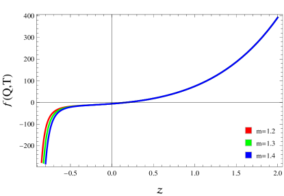
Figure 1: Plot of GDE $f(Q,T)$ model against $z$.

4 Cosmological Analysis

In this section, we will discuss how the universe has evolved through various phases. For this purpose, we employ the reconstructed GDE $f(Q,T)$ model in the non-interacting case (58). We also illustrate the behavior of some cosmological parameters such as the EoS parameter, state finder and $\omega_{GDE}-\omega^{\prime}_{GDE}$ planes. The stability of this model is also discussed.

4.1 Equation of State Parameter

The EoS of DE can describe the cosmic inflation and expansion of the universe. The condition for an accelerating cosmos is analyzed for $\omega<-\frac{1}{3}$. When $\omega=-1$, it simply corresponds to the cosmological constant, however, the values of $\omega=\frac{1}{3}$ and $\omega=0$ demonstrate the radiation and matter-dominated universe, respectively. Furthermore, phantom scenario is observed by assuming $\omega<-1$. The EoS parameter is expressed by

$$\omega_{GDE}=\frac{P_{eff}}{\rho_{eff}}=\frac{P_{GDE}}{\rho_{GDE}+\rho_{M}}.$$ (59)

Equations (42), (43) and (58) are utilized in the above expression to evaluate the corresponding parameter associated with the reconstructed model as

$$\omega_{GDE} =\bigg{[}\Psi^{-2(1+q)}\bigg{\{}-m^{\frac{5}{2}}\alpha\big{(}\Psi^{2+2q}H_{0}^{2}\big{)}^{\frac{1}{4}}-9m^{3}\bigg{(}\frac{\Psi^{2+2q}\beta^{2}}{m^{2}}\bigg{)}^{\frac{-3m}{8}}+72\sqrt{m}\alpha\big{(}\Psi^{2+2q}$$

$$\times H_{0}^{2}\big{)}^{\frac{5}{4}}+m^{\frac{3}{2}}\alpha\big{(}\Psi^{2+2q}H_{0}^{2}\big{)}^{\frac{1}{4}}(54\Psi^{2+2q}H_{0}^{2})+12\Psi^{2+2q}H_{0}^{2}\bigg{\{}-1-\sqrt{\frac{\rho_{o}}{a_{o}^{3}}}\Psi^{2+2q}$$

$$\times H_{0}^{2}-4\bigg{(}\frac{(\Psi)^{2+2q}H_{0}^{2}}{m^{2}}\bigg{)}^{\frac{-3m}{8}}-2(6\Psi^{2+2q}H_{0}^{2})^{\frac{1}{2}}\}+12m^{2}\bigg{\{}\bigg{(}\frac{(\Psi)^{2+2q}H_{0}^{2}}{m^{2}}\bigg{)}^{\frac{-3m}{8}}$$

$$\times 6(\Psi)^{2+2q}H_{0}^{2}\bigg{\}}+m\Psi^{2+2q}H_{0}^{2}\bigg{\{}87-9\sqrt{\frac{\rho_{o}}{a_{o}^{3}}}+324\Psi^{2+2q}H_{0}^{2}(6\Psi^{2+2q}H_{0}^{2})^{\frac{1}{2}}$$

$$+36\bigg{(}\frac{\Psi^{2+2q}H_{0}^{2}}{m^{2}}\bigg{)}^{\frac{-3m}{8}}\bigg{\}}\bigg{\}}\bigg{]}\bigg{[}6(4+3m)H_{0}^{2}\bigg{\{}\frac{\rho_{o}}{a_{o}^{3}}+\frac{1}{2}\bigg{\{}\Psi^{2+2q}H_{0}^{2}+1-2\sqrt{m}\alpha$$

$$\times\bigg{(}\Psi^{2+2q}H_{0}^{2}\bigg{)}^{\frac{1}{4}}-4\bigg{(}\frac{\Psi^{2+2q}H_{0}^{2}}{m^{2}}\bigg{)}^{\frac{-3m}{8}}\bigg{\}}\bigg{\}}\bigg{]}^{-1}.$$ (60)

Figure 2 illustrates the behavior of EoS parameter against $z$ from which one can find that phantom epoch for current as well as late time cosmic evolution is seen.

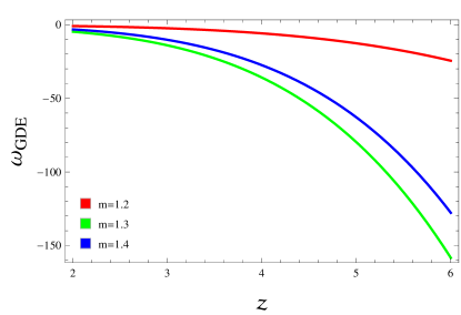
Figure 2: Plot of EoS parameter against $z$.

4.2 $\omega_{GDE}-\omega^{\prime}_{GDE}$ Plane

Here, we utilize the $\omega_{GDE}-\omega^{\prime}_{GDE}$ phase plane, where $\omega^{\prime}_{GDE}$ indicates the evolutionary mode of $\omega_{GDE}$ and prime denotes the derivative with respect to $Q$. This cosmic plane was established by Caldwell and Linder [46] to investigate the quintessence DE paradigm which can be split into freezing $(\omega_{GDE}<0,~{}\omega^{\prime}_{GDE}<0)$ and thawing $(\omega_{GDE}<0,~{}\omega^{\prime}_{GDE}>0)$ regions. In order to illustrate the current cosmic expansion paradigm, the freezing region indicates more accelerated phase as compared to thawing. The cosmic trajectories of $\omega_{GDE}-\omega^{\prime}_{GDE}$ plane for specific choices of $m$ are shown in Figure 3 which provides the freezing region of the cosmos. The expression of $\omega^{\prime}_{GDE}$ is given in Appendix D.

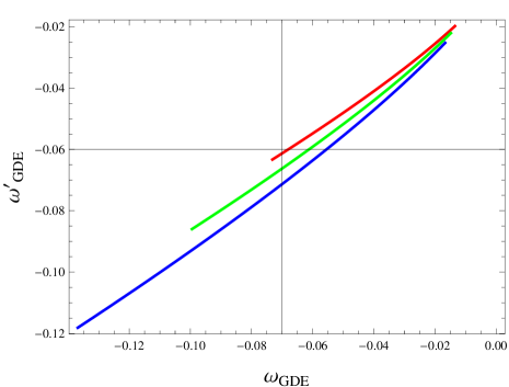
Figure 3: Plot of $\omega_{GDE}-\omega^{\prime}_{GDE}$ versus $z$.

4.3 State Finder Analysis

One of the techniques to examine the dynamics of the cosmos using a cosmological perspective is state finder analysis. It is an essential approach for understanding numerous DE models. As a combination of the Hubble parameter and its temporal derivatives, Sahni et al. [27] established two dimensionless parameters $(r,s)$ given as

$$r=\frac{\dddot{a}}{aH^{3}},\quad s=\frac{r-1}{3(q-\frac{1}{2})}.$$ (61)

The acceleration of cosmic expansion is specified by parameter $s$ whereas the deviation from pure power-law behavior is specifically defined by the parameter $r$. It is a geometric diagnostic that does not support any specific cosmological paradigm. Secondly, it is such an approach that does not depend upon any specific model to distinguish between numerous DE scenarios, i.e., CG (Chaplygin gas), HDE (Holographic DE), SCDM (standard CDM) and quintessence.

Several DE scenarios for the appropriate choices of $r$ and $s$ parametric values are given below.

• When $r=1$, $s=0$, it indicates the CDM model.

• If $r=1$, $s=1$, then it denotes SCDM epoch.

• When $r=1$, $s=\frac{2}{3}$, this epoch demonstrates the HDE model.

• When we have $r>1$, $s<0$, we get CG scenario.

• Lastly, $r<1$, $s>0$ corresponds to quintessence paradigm.

For our considered setup, the parameters $r$ and $s$ in terms of required factors are given in Appendix E. The left plot of Figure 4 indicates the behavior of $r$ versus $z$ while the right plot analyzes $s$ and $z$. The graphical analysis of $r-s$ phase plane in Figure 5 gives $r>1$ and $s<0$, indicating the CG model.

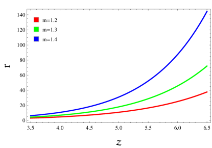
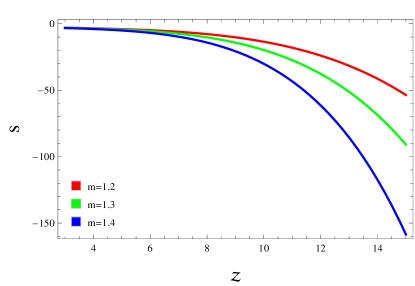
Figure 4: Plots of $r$ against $z$ (left) and $s$ against $z$ (right).

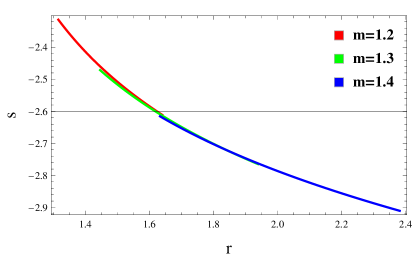
Figure 5: Plot of $r-s$ plane against $z$.

4.4 Squared Speed of Sound Parameter

Stability analysis is a vital concept in understanding the structure and behavior of the cosmos. In this regard, we consider the squared speed of sound parameter to examine the stability of the GDE $f(Q,T)$ model given as

$$\nu_{s}^{2}=\frac{P_{GDE}}{\rho^{\prime}_{GDE}}\omega^{\prime}_{GDE}+\omega_{GDE}.$$ (62)

Its positive value corresponds to the stable configuration whereas the negative value implies unstable behavior for the analogous model. Substituting the required expressions on the right hand side of the above equation for the reconstructed model, we obtain the squared speed of sound parameter given in Appendix E. Figure 6 shows that the speed component is positive for all the assumed values of $m$ and thus the reconstructed GDE $f(Q,T)$ model is stable throughout the cosmic evolution.

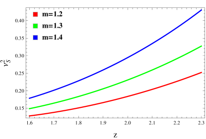
Figure 6: Plot of $\nu_{s}^{2}$ against $z$ for non-interacting case.

5 Final Remarks

In the current scenario, DE is referred to as a vital representative which tends to accelerate the expansion of the universe. In this work, we have examined several characteristics of GDE model within the context of recently developed $f(Q,T)$ theory of gravity. To understand the role of $Q$ and $T$ in GDE ansatz, we have assumed a particular $f(Q,T)=f_{1}(Q)+f_{2}(T)$ model. We have established a reconstruction paradigm using a power-law scale factor as well as a correspondence scenario for a flat FRW universe. We have then investigated the EoS parameter, state finder, $\omega_{GDE}-\omega^{\prime}_{GDE}$ planes and squared sound speed analysis for our derived model. For the graphical representation, we have specified some values to the involved unknowns. The summary of the results is given as follows.

• For non-interacting case, the reconstructed GDE $f(Q,T)$ model reveals an increasing trend with convergence to zero from both sides (Figure 1).

• The EoS parameter indicates an enormous phantom epoch of the universe (Figure 2).

• The trajectories of the $\omega_{GDE}-\omega^{\prime}_{GDE}$ plane depicts the freezing region as both the parameters lie below the zero range (Figure 3).

• The curvatures of $r-s$ plane illustrates CG model because $r$ and $s$ have fulfilled the corresponding model requirements (Figure 5).

• The squared speed of sound parameter indicates a stable regime throughout the cosmic evolutionary paradigm (Figure 6).

We have observed that for suitable choices of free parameters, our reconstructed GDE $f(Q,T)$ model shows consistency with accelerated expanding phenomenon of the universe. According to a review of current observational data [47], the EoS parameter reveals a stable trend when

$$\omega=-1.03\pm 0.03\quad(\text{Planck TT, TE, EE + LowE + lensing + SNe + BAO}).$$

This value has been determined through several kinds of observational techniques, with a 68$\%$ confidence level. Furthermore, we have examined that the cosmic diagnostic state finder parameters for our obtained model correspond to the constraints and restrictions on the kinematics of the cosmos [48]. Sharif and Saba [39] established the correspondence of $f(G)$ theory with GDE paradigm and found that phantom phase for the EoS parameter in non-interacting case. Our results are consistent with these outcomes. Myrzakulov et al. [40] discussed the correspondence between $f(Q)$ and GDE model and found that the reconstructed model is stable while the EoS parameters crosses the phantom divide line. Our results are also consistent with these consequences.

Appendix A: Evaluation of $Q=-Q_{\rho\alpha\beta}P^{\rho\alpha\beta}$

By considering Eq.(8), we can write

$$-g^{\alpha\beta}\mathcal{L}^{\rho}_{\mu\alpha}\mathcal{L}^{\mu}_{\beta\rho} =-\frac{1}{4}g^{\alpha\beta}g^{\rho\lambda}g^{\mu\zeta}(Q_{\alpha\mu\lambda}+Q_{\mu\lambda\alpha}-Q_{\lambda\alpha\mu})(Q_{\rho\beta\zeta}+Q_{\beta\zeta\rho}-Q_{\zeta\rho\beta})$$

$$=-\frac{1}{4}(Q^{\beta\zeta\rho}+Q^{\zeta\rho\beta}-Q^{\rho\beta\zeta})(Q_{\rho\beta\zeta}+Q_{\beta\zeta\rho}-Q_{\zeta\rho\beta})$$

$$=-\frac{1}{4}(2Q^{\rho\beta\zeta}Q_{\zeta\rho\beta}-Q^{\rho\beta\zeta}Q_{\rho\beta\zeta}),$$ (A1)

$$g^{\alpha\beta}\mathcal{L}^{\rho}_{\mu\rho}\mathcal{L}^{\mu}_{\alpha\beta} =\frac{1}{4}g^{\alpha\beta}g^{\mu\zeta}Q_{\mu}(Q_{\beta\alpha\zeta}+Q_{\alpha\zeta\beta}-Q_{\zeta\beta\alpha})=\frac{1}{4}Q^{\zeta}(2\tilde{Q}_{\zeta}-Q_{\zeta}),$$

$$Q =-\frac{1}{4}(-Q^{\rho\beta\zeta}Q_{\rho\beta\zeta}+2Q^{\rho\beta\zeta}Q_{\zeta\rho\beta}-2Q^{\zeta}\tilde{Q}_{\zeta}+Q^{\zeta}{Q}_{\zeta}).$$ (A3)

We can also find $Q$ as follows. Using Eq.(8) in (22), we have

$$P^{\rho\alpha\beta} = \frac{1}{4}\bigg{[}-Q^{\rho\alpha\beta}+Q^{\alpha\rho\beta}+Q^{\beta\rho\alpha}+Q^{\rho}g^{\alpha\beta}-\tilde{Q}^{\rho}g^{\alpha\beta}-\frac{1}{2}(g^{\rho\alpha}Q^{\beta}+g^{\rho\beta}Q^{\alpha}\bigg{]},$$ (A4)

$$-Q_{\rho\alpha\beta}P^{\rho\alpha\beta} = -\frac{1}{4}\bigg{[}-Q_{\rho\alpha\beta}Q^{\rho\alpha\beta}+Q_{\rho\alpha\beta}Q^{\beta\rho\alpha}+Q_{\rho\alpha\beta}Q^{\beta\rho\alpha}$$ (A5)

$$+ Q_{\rho\alpha\beta}Q^{\rho}g^{\alpha\beta}-Q_{\rho\alpha\beta}\tilde{Q}^{\rho}g^{\alpha\beta}-\frac{1}{2}Q_{\rho\alpha\beta}(g^{\rho\alpha}Q^{\beta}+g^{\rho\beta}Q^{\alpha})\bigg{]}$$

$$= -\frac{1}{4}(-Q_{\rho\alpha\beta}Q^{\rho\alpha\beta}+2Q_{\rho\alpha\beta}Q^{\alpha\rho\beta}+Q_{\rho}Q^{\rho}-2Q_{\rho}\tilde{Q^{\rho}})$$

$$= Q.$$

We have used the relations, $Q_{\rho\alpha\beta}Q^{\alpha\rho\beta}=Q_{\rho\alpha\beta}Q^{\beta\rho\alpha}$ to obtain the above results since $Q_{\rho\alpha\beta}Q^{\alpha\rho\beta}=Q_{\rho\beta\alpha}Q^{\alpha\rho\beta}=Q_{\alpha\rho\beta}Q^{\rho\beta\alpha}=Q_{\rho\beta\alpha}Q^{\beta\alpha\rho}Q_{\rho\alpha\beta}Q^{\beta\rho\alpha}$.

Appendix B: Steps for the Variation of $\delta Q$

The formulas related to non-metricity tensors used in the derivation of $\delta Q$ are given as follows

$$Q_{\rho\alpha\beta} =\nabla_{\rho}g_{\alpha\eta},$$

$$Q^{\rho}_{~{}\alpha\beta} =g^{\rho\mu}Q_{\mu\alpha\beta}=g^{\rho\mu}\nabla_{\mu}g_{\alpha\beta}=\nabla^{\rho}g_{\alpha\beta},$$

$$Q^{~{}~{}\mu}_{\rho~{}~{}\beta} =g^{\alpha\zeta}Q_{\rho\zeta\beta}=g^{\alpha\zeta}\nabla_{\rho}g_{\zeta\beta}=-g_{\zeta\beta}\nabla_{\rho}g^{\alpha\zeta},$$

$$Q_{\rho\alpha}^{~{}~{}\beta} =g^{\beta\zeta}Q_{\rho\alpha\zeta}=g^{\beta\zeta}\nabla_{\rho}g_{\alpha\zeta}=-g_{\alpha\zeta}\nabla_{\rho}g^{\beta\zeta},$$

$$Q^{\rho\alpha}_{~{}~{}\beta} =g^{\rho\mu}g^{\alpha\zeta}\nabla_{\mu}g_{\zeta\beta}=g^{\alpha\zeta}\nabla^{\rho}g_{\zeta\beta}=-g_{\zeta\beta}\nabla^{\rho}g^{\alpha\zeta},$$

$$Q^{\rho~{}~{}\beta}_{~{}\alpha} =g^{\rho\mu}g^{\beta\zeta}\nabla_{\mu}g_{\alpha\zeta}=g^{\beta\zeta}\nabla^{\rho}g_{\alpha\zeta}=-g_{\alpha\zeta}\nabla^{\rho}g^{\beta\zeta},$$

$$Q_{\rho}^{\quad\alpha\beta} =g^{\alpha\zeta}g^{\beta\phi}\nabla_{\rho}g_{\zeta\phi}=-g^{\mu\zeta}g_{\zeta\phi}\nabla_{\rho}g^{\beta\phi}=-\nabla_{\rho}g^{\alpha\beta},$$

$$Q^{\rho\alpha\beta} =-\nabla^{\rho}g^{\alpha\beta}.$$

Now, let us find the variation of $Q$ using Eq.(A3) as

$$\delta Q =-\frac{1}{4}\delta(-Q^{\rho\beta\zeta}Q_{\rho\beta\zeta}+2Q^{\rho\beta\zeta}Q_{\zeta\rho\beta}-2Q^{\zeta}\tilde{Q}_{\zeta}+Q^{\zeta}Q_{\zeta})$$

$$=-\frac{1}{4}(-\delta Q^{\rho\beta\zeta}Q_{\rho\beta\zeta}-Q^{\rho\beta\zeta}\delta Q_{\rho\beta\zeta}+2\delta Q^{\rho\beta\zeta}Q_{\zeta\rho\beta}$$

$$+2Q^{\rho\beta\zeta}\delta Q_{\zeta\rho\beta}-2\delta Q^{\zeta}\tilde{Q}_{\zeta}-2Q^{\zeta}\delta\tilde{Q}_{\zeta}+\delta Q^{\zeta}Q_{\zeta}+Q^{\zeta}\delta Q_{\zeta}$$

$$=-\frac{1}{4}\bigg{[}Q_{\rho\beta\zeta}\nabla^{\rho}\delta g^{\beta\zeta}-Q^{\rho\beta\zeta}\nabla_{\rho}\delta g_{\beta\zeta}-2Q_{\zeta\rho\beta}\nabla^{\rho}\delta g^{\beta\zeta}$$

$$+2Q^{\rho\beta\zeta}\nabla_{\zeta}\delta g_{\rho\beta}-2\hat{Q}_{\zeta}\delta(-g_{\alpha\beta}\nabla^{\zeta}g^{\alpha\beta})-2Q^{\zeta}\delta(\nabla^{\lambda}g_{\zeta\lambda})$$

$$+Q_{\zeta}\delta(-g_{\alpha\beta}\nabla^{\zeta}g^{\alpha\beta})+Q^{\zeta}\delta(-g_{\alpha\beta}\nabla_{\zeta}g^{\alpha\beta})\bigg{]}$$

$$=-\frac{1}{4}\bigg{[}Q_{\rho\beta\zeta}\nabla^{\rho}\delta g^{\beta\zeta}-Q^{\rho\beta\zeta}\nabla_{\rho}\delta g_{\beta\zeta}-2Q_{\zeta\rho\beta}\nabla^{\rho}\delta g^{\beta\zeta}$$

$$+2Q^{\rho\beta\zeta}\nabla_{\zeta}\delta g_{\rho\beta}+2\hat{Q}_{\zeta}\nabla^{\zeta}g^{\alpha\beta}\delta g_{\alpha\beta}+2\hat{Q}_{\zeta}g_{\alpha\beta}\nabla^{\zeta}\delta g^{\alpha\beta}$$

$$-2Q^{\zeta}\nabla^{\lambda}\delta g_{\zeta\lambda}-Q_{\zeta}\nabla^{\zeta}g^{\alpha\beta}\delta g_{\alpha\beta}-Q_{\zeta}g_{\alpha\beta}\nabla^{\zeta}\delta g^{\alpha\beta}$$

$$-Q^{\zeta}\nabla_{\zeta}g^{\alpha\beta}\delta g_{\alpha\beta}-Q^{\zeta}g_{\alpha\beta}\nabla_{\zeta}\delta g^{\alpha\beta}\bigg{]}.$$

To simplify the above equation, we employ several useful formulas given as

$$\delta g_{\alpha\beta} =-g_{\alpha\rho}\delta g^{\rho\mu}g_{\mu\beta},$$

$$-Q^{\rho\beta\zeta}\nabla_{\rho}\delta g_{\beta\zeta} =-Q^{\rho\beta\zeta}\nabla_{\rho}(-g_{\beta\lambda}\delta g^{\lambda\theta}g_{\theta\zeta})=2Q^{\rho\beta}_{\quad\theta}Q_{\rho\beta\lambda}\delta g^{\lambda\theta}+Q_{\rho\lambda\theta}\nabla^{\rho}g^{\lambda\theta}$$

$$=2Q^{\rho\phi}_{\quad\beta}Q_{\rho\phi\alpha}\delta g^{\alpha\beta}+Q_{\rho\beta\zeta}\nabla^{\rho}g^{\beta\zeta},$$

$$2Q^{\rho\beta\zeta}\nabla_{\zeta}\delta g_{\rho\beta} =-4Q_{\alpha}^{\quad\phi\zeta}Q_{\zeta\phi\beta}\delta g^{\alpha\beta}-2Q_{\beta\zeta\rho}\nabla^{\rho}\delta g^{\beta\zeta},$$

$$-2Q^{\zeta}\nabla^{\lambda}\delta g_{\zeta\lambda} =2Q^{\rho}Q_{\beta\rho\alpha}\delta g^{\alpha\beta}+2Q_{\alpha}\tilde{Q}_{\beta}\delta g^{\alpha\beta}+2Q_{\beta}g_{\rho\zeta}\nabla^{\rho}g^{\beta\zeta}.$$

Thus, we have

$$\delta Q=2P_{\rho\beta\zeta}\nabla^{\rho}g^{\beta\zeta}-(P_{\alpha\rho\mu}Q_{\beta}^{\quad\alpha\beta}-2Q^{\alpha\beta}_{\quad\alpha}P_{\rho\mu\beta})\delta g^{\alpha\beta},$$

where

$$2P_{\rho\beta\zeta} =-\frac{1}{4}\bigg{[}2Q_{\rho\beta\zeta}-2Q_{\zeta\rho\beta}-2Q_{\beta\zeta\rho}+2(\tilde{Q}_{\rho}-Q_{\rho})g_{\beta\zeta}+2Q_{\beta}g_{\rho\zeta}\bigg{]},$$ (B1)

and

$$4(P_{\alpha\rho\mu}Q_{\beta}^{\quad\alpha\beta}-2Q^{\rho\mu}_{\quad\alpha}P_{\rho\mu\beta}) =2Q^{\alpha\beta}_{\quad\beta}Q_{\rho\mu\beta}-4Q_{\alpha}^{\quad\alpha\beta}Q_{\mu\rho\beta}+2\tilde{Q}^{\rho}Q_{\rho\alpha\beta}\$$

$$+2Q^{\rho}Q^{\beta\rho\alpha}+2Q_{\alpha}\tilde{Q}_{\beta}-Q^{\rho}Q_{\rho\alpha\beta}.$$ (B2)

Appendix C: Calculation of $Q=6H^{2}$

Using Eq.(A5), we have

$$Q=-\frac{1}{4}\big{[}-Q_{\rho\alpha\beta}Q^{\rho\alpha\beta}+2Q_{\rho\alpha\beta}Q^{\alpha\rho\beta}-2\tilde{Q}^{\rho}Q_{\rho}+Q^{\rho}Q_{\rho}\big{]},$$ (C1)

in which

$$-Q_{\rho\alpha\beta}Q^{\rho\alpha\beta} =\nabla_{\rho}g_{\alpha\beta}\nabla^{\rho}g^{\alpha\beta}=12H^{2},$$

$$Q_{\rho\alpha\beta}Q^{\alpha\rho\beta} =-\nabla_{\rho}g_{\alpha\beta}\nabla^{\alpha}g^{\rho\beta}=0,$$

$$\tilde{Q}^{\rho}Q_{\rho} =(g_{\alpha\zeta}\nabla_{\rho}g^{\alpha\zeta})(\nabla_{\mu}g^{\rho\mu})=0,$$

$$Q^{\rho}Q_{\rho} =(g_{\zeta\alpha}\nabla_{\rho}g^{\zeta\alpha})(g_{\phi\beta}\nabla^{\rho}g^{\zeta\beta})=-36H^{2}.$$

Substituting all the above expressions in (C1), it follows that

$$Q =6H^{2}.$$

Appendix D: Calculation of $\omega^{\prime}_{GDE}$

$$\omega^{\prime}_{GDE}= -\bigg{[}\Psi^{-2(1+q)}\bigg{\{}-\frac{3m^{\frac{5}{2}}(2+2q)\Psi^{1+2q}\alpha\beta^{2}}{4\big{(}\Psi^{2+2q}H_{0}^{2}\big{)}^{\frac{3}{4}}}+90\sqrt{m}(2+2q)\Psi^{1+2q}\alpha H_{0}^{2}$$

$$\times\big{(}\Psi^{2+2q}H_{0}^{2}\big{)}^{\frac{1}{4}}+54m^{\frac{3}{2}}(2+2q)\Psi^{1+2q}\alpha H_{0}^{2}(\Psi^{2+2q}H_{0}^{2})^{\frac{1}{4}}+m^{2}\Psi^{1+2q}H_{0}^{2}$$

$$\times(2+2q)\big{(}\Psi^{2+2q}H_{0}^{2}{m^{2}}\big{)}^{\frac{-3m}{8}}+m^{\frac{3}{2}}(2+2q)\Psi^{1+2q}\alpha H_{0}^{2}(-4+54\Psi^{2+2q}H_{0}^{2})$$

$$\times\bigg{\{}\big{(}\Psi^{2+2q}4H_{0}^{2}\big{)}^{\frac{3}{4}}+m\Psi^{2+2q}H_{0}^{2}\bigg{\{}\sqrt{6}(2+2q)\Psi^{1+2q}H_{0}^{2}\sqrt{\Psi^{2+2q}H_{0}^{2}}\Psi^{1+2q}$$

$$\times H_{0}^{2}-\frac{1}{2m}27(2+2q)\bigg{(}\frac{\Psi^{2+2q}H_{0}^{2}}{{m^{2}}}\bigg{)}^{-1-\frac{3m}{8}}\bigg{\}}\Psi^{1+2q}H_{0}^{2}+12m^{2}\bigg{\{}6(2+2q)$$

$$\times\Psi^{1+2q}H_{0}^{2}+\frac{1}{8m}3(2+2q)H_{0}^{2}\Psi^{1+2q}\Psi^{1+2q}\bigg{(}\frac{\Psi^{2+2q}H_{0}^{2}}{{m^{2}}}\bigg{)}^{{-1-\frac{3m}{8}}}\bigg{\}}+12\Psi^{2+2q}$$

$$\times H_{0}^{2}\bigg{\{}(2+2q)\Psi^{1+2q}H_{0}^{2}-\frac{\sqrt{6}(2+2q)\Psi^{1+2q}H_{0}^{2}}{\sqrt{\Psi}^{2+2q}H_{0}^{2}}+\frac{3}{2m}(2+2q)\Psi^{1+2q}$$

$$\times H_{0}^{2}\bigg{(}\frac{\Psi^{2+2q}H_{0}^{2}}{m^{2}}\bigg{)}^{-1-\frac{3m}{8}}\bigg{\}}+\Psi^{2+2q}H_{0}^{2}\bigg{\{}36(2+2q)\Psi^{1+2q}+\bigg{(}\frac{\Psi^{2+2q}H_{0}^{2}}{{m^{2}}}\bigg{)}^{\frac{-3m}{8}}$$

$$\times 3\Psi^{1+2q}H_{0}^{2}-\frac{\sqrt{6}(2+2q)\Psi^{1+2q}H_{0}^{2}}{\sqrt{\Psi^{2+2q}H_{0}^{2}}}(2+2q)\frac{1}{2m}H_{0}^{2}\bigg{\}}+12(2+2q)\Psi^{1+2q}$$

$$\times H_{0}^{2}\bigg{\{}1-\sqrt{\frac{\rho_{o}}{a_{o}^{3}}}+\Psi^{2+2q}+36H_{0}^{2}-2\sqrt{6}\sqrt{\Psi^{2+2q}H_{0}^{2}}-4\bigg{(}\frac{\Psi^{2+2q}H_{0}^{2}}{m^{2}}\bigg{)}^{\frac{-3m}{8}}\bigg{\}}$$

$$+m(2+2q)\Psi^{1+2q}H_{0}^{2}\bigg{\{}87-9\sqrt{\frac{\rho_{o}}{a_{o}^{3}}}+(\Psi)^{2+2q}H_{0}^{2}-18\sqrt{6}\sqrt{(\Psi)}^{2+2q}H_{0}^{2}$$

$$+36\bigg{(}\frac{\Psi^{2+2q}H_{0}^{2}}{m^{2}}\bigg{)}^{-3\frac{m}{8}}\bigg{\}}\bigg{\}}\bigg{]}\bigg{[}6(4+3m)H_{0}^{2}\bigg{\{}\frac{\rho_{o}}{a_{o}^{3}}+\bigg{\{}\frac{1}{2}\bigg{(}-1-12H_{0}^{2}\Psi^{2+2q}$$

$$+2\alpha\big{(}\Psi^{2+2q}H_{0}^{2}\big{)}^{\frac{1}{4}}-4\bigg{(}\frac{\Psi^{2+2q}H_{0}^{2}}{m^{2}}\bigg{)}^{-3\frac{m}{8}}\bigg{\}}\bigg{\}}\bigg{\}}\bigg{]}^{-1}+\bigg{\{}\Psi^{-2(1+q)}\bigg{\{}\Psi^{1+2q}H_{0}^{2})$$

$$\times(2+2q)+\frac{\sqrt{m}(2+2q)\Psi^{1+2q}\alpha H_{0}^{2}}{2(\Psi^{2+2q}H_{0}^{2})^{\frac{3}{4}}}\bigg{\}}\bigg{\{}\frac{1}{2m}(3(2+2q)\Psi^{1+2q}H_{0}^{2}-3m^{\frac{5}{2}}$$

$$+\bigg{(}\frac{\Psi^{2+2q}H_{0}^{2}}{m^{2}}\bigg{)}^{-1\frac{-3m}{8}}(\alpha\Psi^{2+2q}H_{0}^{2})^{\frac{1}{4}}+\sqrt{m}\alpha(\Psi^{2+2q}H_{0}^{2})^{\frac{5}{4}}-m^{3}\bigg{(}\frac{\Psi^{2+2q}H_{0}^{2}}{m^{2}}\bigg{)}^{\frac{-3m}{8}}$$

$$+390m^{\frac{3}{2}}\alpha(\Psi^{2+2q}H_{0}^{2})^{\frac{1}{4}}(-4+54\Psi^{2+2q}H_{0}^{2})+12\Psi^{2+2q}H_{0}^{2}\bigg{\{}-1-\sqrt{\frac{\rho_{0}}{a_{0}^{3}}}$$

$$+36\Psi^{2+2q}H_{0}^{2}-2\sqrt{6}\sqrt{\Psi^{2+2q}H_{0}^{2}}+72\alpha\sqrt{m}-4\bigg{(}\frac{\Psi^{2+2q}H_{0}^{2}}{m^{2}}\bigg{)}^{-3\frac{m}{8}}\bigg{\}}+\bigg{\{}\Psi^{2+2q}$$

$$\times H_{0}^{2})-\bigg{(}\frac{\Psi^{2+2q}H_{0}^{2}}{m^{2}}\bigg{)}^{\frac{-3m}{8}}\bigg{\}}12m^{2}+m\Psi^{2+2q}H_{0}^{2}\bigg{\{}87-9\sqrt{\frac{\rho_{0}}{a_{0}^{3}}}+324\Psi^{2+2q}$$

$$\times H_{0}^{2}-18\sqrt{6}\sqrt{\Psi^{2+2q}H_{0}^{2}}+36\bigg{(}\frac{\Psi^{2+2q}H_{0}^{2}}{m^{2}}\bigg{)}^{-3\frac{m}{8}}\bigg{\}}\bigg{\}}\bigg{\}}+((1+z)^{2+2q}H_{0}^{2})^{\frac{1}{4}}$$

$$\times\bigg{\{}12(4+3m)H_{0}^{2}\bigg{[}\frac{\rho_{0}}{a_{0}^{3}}+\frac{1}{2}\bigg{\{}-1-H_{0}^{2}+\alpha(\Psi^{2+2q}H_{0}^{2})^{\frac{1}{4}}-4\bigg{(}\frac{\Psi^{2+2q}H_{0}^{2}}{m^{2}}\bigg{)}^{\frac{-3m}{8}}$$

$$\times\Psi^{2+2q}\bigg{\}}\bigg{]}^{2}\bigg{\}}+\bigg{\{}(1+q)\Psi^{-1-2(1+q)}\bigg{\{}-3m^{\frac{5}{2}}\alpha\big{(}\Psi^{2+2q}H_{0}^{2}\big{)}^{\frac{1}{4}}+72\sqrt{m}\alpha$$

$$\times\bigg{(}\Psi^{2+2q}H_{0}^{2}\bigg{)}^{\frac{5}{4}}-\bigg{(}\frac{(\Psi)^{2+2q}H_{0}^{2}}{m^{2}}\bigg{)}^{\frac{-3m}{8}}\times m^{\frac{3}{2}}\alpha((1+z)^{2+2q}H_{0}^{2})^{\frac{1}{4}}(-4$$

$$+54(\Psi)^{2+2q}H_{0}^{2}+12\sqrt{m}\alpha(\Psi)^{2+2q}H_{0}^{2}\bigg{\{}-1-\sqrt{\frac{\rho_{0}}{a_{0}^{3}}}+36\Psi^{2+2q}H_{0}^{2}-2$$

$$\times\sqrt{6}\sqrt{(\Psi)^{2+2q}H_{0}^{2}}+12\sqrt{m}\alpha-4\bigg{(}\frac{\Psi^{2+2q}H_{0}^{2}}{m^{2}}\bigg{)}^{-3\frac{m}{8}}\bigg{\}}+\bigg{\{}6\Psi^{2+2q}H_{0}^{2}$$

$$-\bigg{(}\frac{\Psi^{2+2q}H_{0}^{2}}{m^{2}}\bigg{)}^{-3\frac{m}{8}}12m^{2}\bigg{\}}+m(\Psi)^{2+2q}H_{0}^{2}\bigg{\{}87-9\sqrt{\frac{\rho_{0}}{a_{0}^{3}}}+324\sqrt{m}\Psi^{2+2q}$$

$$-18\sqrt{6}\sqrt{(\Psi)^{2+2q}\beta}^{2}H_{0}^{2}+\times 36(\frac{((\Psi)^{2+2q}H_{0}^{2}}{m^{2}})^{-3\frac{m}{8}}\bigg{\}}\bigg{\}}\bigg{\}}\bigg{[}3(4+3m)H_{0}^{2}$$

$$\times\bigg{\{}\frac{\rho_{0}}{a_{0}^{3}}+\frac{1}{2}\bigg{\{}-1-12(\Psi)^{2+2q}H_{0}^{2}-4\bigg{(}\frac{\Psi^{2+2q}H_{0}^{2}}{m^{2}}\bigg{)}^{\frac{-3m}{8}}-2\sqrt{m}\alpha((\Psi)^{2+2q}$$

$$\times H_{0}^{2})^{\frac{1}{4}}\bigg{\}}\bigg{\}}\bigg{]}^{-1}.$$ (D1)

Appendix E: Evaluation of $r$ and $s$ Parameters

$$r =\frac{1}{4}\bigg{[}2-\bigg{\{}\Psi^{-2(1+q)}\bigg{\{}-3m^{\frac{5}{2}}\alpha(\Psi^{2+2q}H_{0}^{2})^{\frac{1}{4}}-9m^{3}\bigg{(}\frac{\Psi^{2+2q}H_{0}^{2}}{m^{2}}\bigg{)}^{-3\frac{m}{8}}+(\Psi^{2+2q}$$

$$\times H_{0}^{2})^{\frac{5}{4}}+72\sqrt{m}\alpha+\big{(}-4+54\Psi^{2+2q}H_{0}^{2}\big{)}m^{\frac{3}{2}}72\sqrt{\alpha}\big{(}(\Psi)^{2+2q}H_{0}^{2}\big{)}^{\frac{1}{4}}+12\Psi^{2+2q}$$

$$\times H_{0}^{2}\bigg{\{}-1-\sqrt{\frac{\rho_{o}}{a_{o}^{3}}}+36m^{2}\Psi^{2+2q}H_{0}^{2}-2(6(\Psi)^{2+2q}H_{0}^{2})^{\frac{1}{2}}-4\bigg{(}\frac{\Psi^{2+2q}H_{0}^{2}}{m^{2}}\bigg{)}^{-3\frac{m}{8}}\bigg{\}}$$

$$+12m^{2}\bigg{\{}6(\Psi)^{2+2q}H_{0}^{2}-\bigg{(}\frac{(\Psi)^{2+2q}H_{0}^{2}}{m^{2}}\bigg{)}^{-3\frac{m}{8}}\bigg{\}}+m\Psi^{2+2q}H_{0}^{2}\bigg{\{}87-\sqrt{(\Psi)^{2+2q}H_{0}^{2}}$$

$$\times 18\sqrt{6}-9\sqrt{\frac{\rho_{o}}{a_{o}^{3}}}+324\Psi^{2+2q}H_{0}^{2}+36\bigg{(}\frac{(\Psi)^{2+2q}H_{0}^{2}}{m^{2}}\bigg{)}^{-3\frac{m}{8}}\bigg{\}}\bigg{\}}\bigg{\}}\bigg{[}(4+3m)H_{0}^{2}\bigg{\{}\frac{\rho_{o}}{a_{o}^{3}}$$

$$+\frac{1}{2}\bigg{\{}-1-\Psi^{2+2q}H_{0}^{2}+\sqrt{m}\alpha((\Psi)^{2+2q}H_{0}^{2})^{\frac{1}{4}}-\bigg{(}(\Psi)^{2+2q}H_{0}^{2}m^{-2}\bigg{)}^{-3\frac{m}{8}}\bigg{\}}\bigg{\}}\bigg{]}^{-1}+8$$

$$\times\bigg{\{}\frac{1}{2}-\bigg{\{}\Psi^{-2(1+q)}\bigg{\{}-3m^{\frac{5}{2}}\alpha\big{(}(\Psi)^{2+2q}H_{0}^{2}\big{)}^{\frac{1}{4}}+\big{(}\Psi^{2+2q}H_{0}^{2}\big{)}^{\frac{5}{4}}+\alpha\big{(}\Psi^{2+2q}H_{0}^{2}\big{)}^{\frac{1}{4}}$$

$$\times 72\sqrt{m}\alpha-m^{3}\big{(}(\Psi)^{2+2q}H_{0}^{2}m^{-2}\big{)}^{\frac{-3m}{8}}(-4+54\Psi^{2+2q}H_{0}^{2})+12(\Psi)^{2+2q}H_{0}^{2}\bigg{\{}-1$$

$$-\sqrt{\frac{\rho_{o}}{a_{o}^{3}}}+36(\Psi)^{2+2q}H_{0}^{2}-(6\Psi^{2+2q}H_{0}^{2})^{\frac{1}{2}}m^{\frac{3}{2}}-\big{(}\Psi^{2+2q}\big{)}^{-3\frac{m}{8}}\big{(}(H_{0}^{2}m^{-2})^{-3\frac{m}{8}}\big{)}\bigg{\}}$$

$$+\bigg{\{}6\Psi^{2+2q}H_{0}^{2}-\bigg{(}\frac{(\Psi)^{2+2q}H_{0}^{2}}{m^{2}}\bigg{)}^{-3\frac{m}{8}}\bigg{\}}12m^{2}+m\Psi^{2+2q}H_{0}^{2}\bigg{\{}324\Psi^{2+2q}H_{0}^{2}-18$$

$$\times(6(\Psi)^{2+2q}H_{0}^{2})^{\frac{1}{2}}87-9\sqrt{\frac{\rho_{0}}{a_{0}^{3}}}+36\bigg{(}\frac{(1+z)^{2+2q}H_{0}^{2}}{m^{2}}\bigg{)}^{-3\frac{m}{8}}\bigg{\}}\bigg{\}}\bigg{\}}\times\bigg{\{}(4+3m)$$

$$\times\bigg{\{}\frac{\rho_{0}}{a_{0}^{3}}+\frac{1}{2}\bigg{\{}-1-12\Psi^{2+2q}H_{0}^{2}+((\Psi)^{2+2q}H_{0}^{2})^{\frac{1}{4}}-\bigg{(}\frac{(\Psi)^{2+2q}H_{0}^{2}}{m^{2}}\bigg{)}^{-3\frac{m}{8}}\Psi^{2+2q}$$

$$\times H_{0}^{2}\bigg{\}}\bigg{\}}\bigg{\}}^{-1}\bigg{]}^{2}-\bigg{\{}(1+q)(1+z)^{-4-3q}\bigg{\{}2\bigg{\{}-24(\Psi)^{2+2q}H_{0}^{2}m^{\frac{3}{2}}\alpha+\sqrt{m}\alpha$$

$$\times\big{(}\Psi^{2+2q}H_{0}^{2}\big{)}^{\frac{1}{4}}+3m\bigg{(}\frac{\Psi^{2+2q}H_{0}^{2}}{m^{2}}\bigg{)}^{-3\frac{m}{8}}\bigg{\}}\bigg{\}}\bigg{\{}-3m^{\frac{5}{2}}\alpha\big{(}(\Psi)^{2+2q}H_{0}^{2}\big{)}^{\frac{1}{4}}+72\sqrt{m}\alpha$$

$$\times\big{(}(\Psi)^{2+2q}H_{0}^{2}\big{)}^{\frac{5}{4}}-m^{3}\bigg{(}\frac{(\Psi)^{2+2q}H_{0}^{2}}{m^{2}}\bigg{)}^{-3\frac{m}{8}}+\big{(}(\Psi)^{2+2q}\big{)}^{\frac{1}{4}}(-4+54(\Psi)^{2+2q}H_{0}^{2})$$

$$+12(\Psi)^{2+2q}H_{0}^{2}\bigg{\{}-2\sqrt{6}\sqrt{(\Psi)^{2+2q}H_{0}^{2}}-\bigg{\{}12m^{2}-\sqrt{\frac{\rho_{0}}{a_{0}^{3}}}+36(\Psi)^{2+2q}H_{0}^{2}-4$$

$$\bigg{(}\frac{\Psi^{2+2q}H_{0}^{2}}{m^{2}}\bigg{)}^{-3\frac{m}{8}}\bigg{\}}+12m^{2}\bigg{\{}6\Psi^{2+2q}H_{0}^{2}-\bigg{(}\frac{(\Psi)^{2+2q}H_{0}^{2}}{m^{2}}\bigg{)}^{-3\frac{m}{8}}\bigg{\}}+m\Psi^{2+2q}H_{0}^{2}$$

$$\times\bigg{\{}87-9\sqrt{\frac{\rho_{0}}{a_{0}^{3}}}+324(\Psi)^{2+2q}H_{0}^{2}-18(6(\Psi)^{2+2q}H_{0}^{2})^{\frac{1}{2}}+\big{(}(\Psi^{2+2q}H_{0}^{2}m^{-2}\big{)}^{\frac{-3m}{8}}\bigg{\}}\bigg{\}}$$

$$+8\bigg{\{}{\frac{\rho_{0}}{a_{0}^{3}}}+\bigg{\{}(\Psi)^{2+2q}H_{0}^{2}+2\sqrt{m}\alpha\big{(}(\Psi)^{2+2q}H_{0}^{2}\big{)}^{\frac{1}{4}})-4\bigg{(}\frac{(\Psi)^{2+2q}H_{0}^{2}}{m^{2}}\bigg{)}^{-3\frac{m}{8}}\bigg{\}}\bigg{\}}$$

$$\times\bigg{\{}-3m^{\frac{5}{2}}\alpha\big{(}(\Psi)^{2+2q}H_{0}^{2}\big{)}^{\frac{1}{4}}+\sqrt{m}\alpha\big{(}(\Psi)^{2+2q}H_{0}^{2}\big{)}^{\frac{5}{4}}-m^{3}\bigg{(}\frac{(\Psi)^{2+2q}H_{0}^{2}}{m^{2}}\bigg{)}^{-3\frac{m}{8}}$$

$$+\big{(}\Psi^{2+2q}H_{0}^{2}\big{)}^{\frac{1}{4}}(-4+54(\Psi)^{2+2q}H_{0}^{2})+12(\Psi)^{2+2q}H_{0}^{2}\bigg{\{}-1-\sqrt{\frac{\rho_{0}}{a_{0}^{3}}}+36(\Psi)^{2+2q}$$

$$\times H_{0}^{2}-2\sqrt{6}\sqrt{(\Psi)^{2+2q}H_{0}^{2}}-4\bigg{(}\frac{(\Psi)^{2+2q}H_{0}^{2}}{m^{2}}\bigg{)}^{-3\frac{m}{8}}\bigg{\}}+12m^{2}\bigg{\{}\bigg{(}\frac{(\Psi)^{2+2q}H_{0}^{2}}{m^{2}}\bigg{)}^{-3\frac{m}{8}}$$

$$\times 6\Psi^{2+2q}H_{0}^{2})\bigg{\}}+m\Psi^{2+2q}H_{0}^{2}\bigg{\{}87-9\sqrt{\frac{\rho_{0}}{a_{0}^{3}}}+324\Psi^{2+2q}H_{0}^{2}\sqrt{(\Psi)^{2+2q}H_{0}^{2}}-18\sqrt{6}$$

$$+36\big{(}(\Psi)^{2+2q}H_{0}^{2}m^{-2}\big{)}^{-3\frac{m}{8}}\bigg{\}}\bigg{\}}-\bigg{\{}{\frac{\rho_{0}}{a_{0}^{3}}}+\frac{1}{2}\bigg{\{}-12(\Psi)^{2+2q}H_{0}^{2})+\big{(}(\Psi)^{2+2q}H_{0}^{2}\big{)}^{\frac{1}{4}}$$

$$\times 2\sqrt{m}\alpha-4\bigg{(}\frac{(\Psi)^{2+2q}H_{0}^{2}}{m^{2}}\bigg{)}^{-3\frac{m}{8}}\bigg{\}}\bigg{\}}\bigg{\{}-6m^{\frac{5}{2}}\alpha\big{(}(\Psi)^{2+2q}H_{0}^{2}\big{)}^{\frac{1}{4}}+\big{(}\Psi^{2+2q}H_{0}^{2}\big{)}^{\frac{5}{4}}$$

$$+720\sqrt{m}\alpha+m^{\frac{3}{2}}\alpha\big{(}(\Psi)^{2+2q}H_{0}^{2}\big{)}^{\frac{5}{4}}+m^{4}\bigg{(}\frac{(\Psi)^{2+2q}H_{0}^{2}}{m^{2}}\bigg{)}^{-3\frac{m}{8}}+\alpha\big{(}(\Psi)^{2+2q}H_{0}^{2}\big{)}^{\frac{1}{4}}$$

$$+4m^{\frac{3}{2}}(27(\Psi)^{2+2q}H_{0}^{2})+96(\Psi)^{2+2q}H_{0}^{2}\bigg{\{}-\sqrt{\frac{\rho_{0}}{a_{0}^{3}}}+36(\Psi)^{2+2q}H_{0}^{2}-\Psi^{2+2q}H_{0}^{2})^{\frac{1}{2}}$$

$$-4\bigg{(}\frac{(\Psi)^{2+2q}H_{0}^{2}}{m^{2}}\bigg{)}^{-3\frac{m}{8}}\bigg{\}}+8m(\Psi)^{2+2q}H_{0}^{2}\bigg{\{}-\sqrt{\frac{\rho_{o}}{a_{o}^{3}}}-(6\Psi^{2+2q}H_{0}^{2})^{\frac{1}{2}}+(\Psi)^{2+2q}$$

$$\times H_{0}^{2}+\big{(}\Psi^{2+2q}H_{0}^{2}m^{-2}\big{)}^{-3\frac{m}{8}}\bigg{\}}+m(\Psi)^{2+2q}H_{0}^{2}\bigg{\{}72(\Psi)^{2+2q}H_{0}^{2}-\sqrt{(\Psi)^{2+2q}H_{0}^{2}}$$

$$\times 2\sqrt{6}-3m\bigg{(}\frac{(\Psi)^{2+2q}H_{0}^{2}}{m^{2}}\bigg{)}^{-3\frac{m}{8}}\bigg{\}}+m^{2}\bigg{\{}16\Psi^{2+2q}H_{0}^{2}+m\bigg{(}\Psi^{2+2q}H_{0}^{2}m^{-2}\bigg{)}^{-3\frac{m}{8}}\bigg{\}}$$

$$+\Psi^{2+2q}H_{0}^{2}\bigg{\{}72(\Psi)^{2+2q}H_{0}^{2}-\sqrt{(\Psi)^{2+2q}H_{0}^{2}}+3m\bigg{(}\frac{(\Psi)^{2+2q}H_{0}^{2}}{m^{2}}\bigg{)}^{-3\frac{m}{8}}\bigg{\}}\bigg{\}}\bigg{\}}\bigg{\}}$$

$$\times\bigg{[}4(4+3m)\beta^{3}\bigg{\{}{\frac{\rho_{o}}{a_{o}^{3}}}+\frac{1}{2}\bigg{\{}-1-12(\Psi)^{2+2q}H_{0}^{2}+2\sqrt{m}\alpha((\Psi)^{2+2q}H_{0}^{2})^{\frac{1}{4}}$$

$$-4\bigg{(}\frac{(\Psi)^{2+2q}H_{0}^{2}}{m^{2}}\bigg{)}^{-3\frac{m}{8}}\bigg{\}}\bigg{\}}^{2}\bigg{]}^{-1}\bigg{]},$$

$$s =\bigg{[}-4(4+3m)(\Psi)^{2+2q}H_{0}^{2}\bigg{\{}\frac{\rho_{0}}{a_{0}^{3}}+\frac{1}{2}\bigg{\{}-1-4\bigg{(}\frac{(\Psi)^{2+2q}H_{0}^{2}}{m^{2}}\bigg{)}^{\frac{-3m}{8}}-12(\Psi)^{2+2q}$$

$$\times H_{0}^{2}+2\sqrt{m}\alpha\big{(}(\Psi)^{2+2q}H_{0}^{2}\big{)}^{\frac{1}{4}}\bigg{\}}\bigg{\}}-\bigg{\{}\frac{1}{4}\times\bigg{\{}2-\bigg{\{}\Psi^{-2(1+q)}\bigg{\{}-3m^{\frac{5}{2}}\alpha\big{(}\Psi^{2+2q}H_{0}^{2}\big{)}^{\frac{1}{4}}$$

$$-9m^{3}\bigg{(}\frac{\Psi^{2+2q}H_{0}^{2}}{m^{2}}\bigg{)}^{\frac{-3m}{8}}\big{(}\Psi^{2+2q}H_{0}^{2}\big{)}^{\frac{5}{4}}+m^{\frac{3}{2}}\alpha\big{(}(\Psi)^{2+2q}H_{0}^{2}\big{)}^{\frac{1}{4}}(-4+54\Psi^{2+2q}H_{0}^{2})$$

$$+12\Psi^{2+2q}H_{0}^{2}\bigg{\{}\sqrt{\frac{\rho_{0}}{a_{0}^{3}}}+36\Psi^{2+2q}H_{0}^{2}-2\sqrt{6}\sqrt{\Psi^{2+2q}H_{0}^{2}}-4\bigg{(}\frac{\Psi^{2+2q}H_{0}^{2}}{m^{2}}\bigg{)}^{\frac{-3m}{8}}\bigg{\}}+12$$

$$\times m^{2}\bigg{\{}6\Psi^{2+2q}H_{0}^{2}-\bigg{(}\frac{(\Psi)^{2+2q}H_{0}^{2}}{m^{2}}\bigg{)}^{\frac{-3m}{8}}+m\Psi^{2+2q}H_{0}^{2}\bigg{\{}9\sqrt{\frac{\rho_{0}}{a_{0}^{3}}}+324\Psi^{2+2q}H_{0}^{2}-18$$

$$\times\sqrt{6}\sqrt{\Psi^{2+2q}H_{0}^{2}}+36\bigg{(}\frac{\Psi^{2+2q}H_{0}^{2}}{m^{2}}\bigg{)}^{\frac{-3m}{8}}\bigg{\}}\bigg{\}}\bigg{\}}\bigg{[}(4+3m)H_{0}^{2}\bigg{\{}\frac{\rho_{0}}{a_{0}^{3}}+\frac{1}{2}\bigg{\{}-\big{(}\Psi^{2+2q}\beta)^{2}$$

$$+2\sqrt{m}\alpha\big{(}\Psi)^{2+2q}\beta)^{2}\big{)}^{\frac{1}{4}}-4\bigg{(}\frac{((\Psi)^{2+2q}\beta)^{2}}{m^{2}}\bigg{)}^{\frac{-3m}{8}}\bigg{\}}\bigg{\}}\bigg{]}^{-1}+8\bigg{\{}\frac{1}{2}-\bigg{\{}\Psi^{1+q)}\bigg{\{}m^{\frac{5}{2}}$$

$$\times\alpha\big{(}\Psi^{2+2q}H_{0}^{2}\big{)}^{\frac{1}{4}}+72\sqrt{m}\alpha(\Psi^{2+2q}H_{0}^{2})^{\frac{5}{4}})-9m^{3}\bigg{(}\frac{\Psi^{2+2q}H_{0}^{2}}{m^{2}}\bigg{)}^{-3\frac{m}{8}}+\big{(}\Psi^{2+2q}H_{0}^{2}\big{)}^{\frac{1}{4}}$$

$$+m^{\frac{3}{2}}\alpha\bigg{\{}54(\Psi)^{2+2q}H_{0}^{2}+12\Psi^{2+2q}H_{0}^{2}\bigg{\{}-1-\sqrt{\frac{\rho_{0}}{a_{0}^{3}}}+36\Psi^{2+2q}H_{0}^{2}-2\sqrt{6}$$

$$\times\sqrt{\Psi^{2+2q}H_{0}^{2}}-4\bigg{(}\frac{\Psi)^{2+2q}H_{0}^{2}}{m^{2}}\bigg{)}^{\frac{-3m}{8}}\bigg{\}}\bigg{\}}+m^{2}\bigg{\{}6\Psi^{2+2q}H_{0}^{2}-\bigg{(}\frac{(\Psi)^{2+2q}H_{0}^{2}}{m^{2}}\bigg{)}^{\frac{-3m}{8}}\bigg{\}}$$

$$+m\Psi^{2+2q}H_{0}^{2}\bigg{\{}\sqrt{\frac{\rho_{0}}{a}_{0}^{3}}+\Psi^{2+2q}H_{0}^{2}-\sqrt{6}\sqrt{(\Psi)^{2+2q}H_{0}^{2}}+\bigg{(}\frac{\Psi^{2+2q}H_{0}^{2}}{m^{2}}\bigg{)}^{\frac{-3m}{8}}\bigg{\}}\bigg{\}}\bigg{\}}$$

$$\times\bigg{[}4H_{0}^{2}\bigg{\{}\frac{\rho_{0}}{a_{0}^{3}}+\frac{1}{2}\bigg{\{}\Psi^{2+2q}H_{0}^{2}+324m^{2}+2\sqrt{m}\alpha\big{(}\Psi^{2+2q}H_{0}^{2}\big{)}^{\frac{1}{4}}-4\bigg{(}\frac{\Psi^{2+2q}H_{0}^{2}}{m^{2}}\bigg{)}^{\frac{-3m}{8}}$$

$$+12m^{2}\sqrt{\frac{\rho_{0}}{a_{0}^{3}}}\bigg{\}}\bigg{\}}\bigg{]}^{2}\bigg{[}\alpha(\Psi^{2+2q}H_{0}^{2})^{\frac{1}{4}}\bigg{\}}+\sqrt{m}\alpha\big{(}\Psi^{2+2q}H_{0}^{2}\big{)}^{\frac{5}{4}}-9m^{3}\bigg{(}\frac{\Psi^{2+2q}H_{0}^{2}}{m^{2}}\bigg{)}^{\frac{-3m}{8}}$$

$$+m^{\frac{3}{2}}\alpha\big{(}\Psi^{2+2q}H_{0}^{2}\big{)}^{\frac{1}{4}}(-4+54\Psi^{2+2q}H_{0}^{2})+12\Psi^{2+2q}H_{0}^{2}\sqrt{\frac{\rho_{0}}{a_{0}^{3}}}+36\Psi^{2+2q}H_{0}^{2}$$

$$-\sqrt{\Psi^{2+2q}H_{0}^{2}}-4\bigg{(}\frac{\Psi^{2+2q}H_{0}^{2}}{m^{2}}\bigg{)}\Psi^{2+2q}H_{0}^{2}-\bigg{(}\frac{\Psi^{2+2q}H_{0}^{2}}{m^{2}}\bigg{)}^{\frac{-3m}{8}}\bigg{\}}+m(\Psi)^{2+2q}H_{0}^{2}$$

$$-9\sqrt{\frac{\rho_{0}}{a_{0}^{3}}}+324\Psi^{2+2q}H_{0}^{2}-18\sqrt{6}\sqrt{\Psi^{2+2q}H_{0}^{2}}+36\bigg{(}\frac{\Psi^{2+2q}H_{0}^{2}}{m^{2}}\bigg{)}\bigg{\}}\bigg{\}}\bigg{]}^{-1}.$$ (E1)

Appendix F: Determination of $\nu_{s}^{2}$

$$\nu_{s}^{2} =\bigg{[}\Psi^{-2(1+q)}\bigg{\{}-4\bigg{\{}\frac{\rho_{0}}{a_{0}^{3}}+\frac{1}{2}\bigg{\{}2\sqrt{m}\alpha(\Psi^{2+2q}H_{0}^{2})^{\frac{1}{4}}-4\bigg{(}\frac{\Psi^{2+2q}H_{0}^{2}}{m^{2}}\bigg{)}^{\frac{-3m}{8}}\Psi^{2+2q}\bigg{\}}\bigg{\}}$$

$$\times H_{0}^{2}+\bigg{\{}m^{\frac{5}{2}}\alpha(\Psi^{2+2q}H_{0}^{2})^{\frac{1}{4}}+\sqrt{m}\alpha\big{(}\Psi^{2+2q}H_{0}^{2}\big{)}^{\frac{5}{4}}-9m^{3}\bigg{(}\frac{\Psi^{2+2q}H_{0}^{2}}{m^{2}}\bigg{)}^{\frac{-3m}{8}}+m^{\frac{3}{2}}$$

$$\times\alpha(\Psi^{2+2q}H_{0}^{2})^{\frac{1}{4}}(-4+54\Psi^{2+2q}H_{0}^{2})+12\Psi^{2+2q}H_{0}^{2}\bigg{\{}-1-\sqrt{\frac{\rho_{0}}{a_{0}^{3}}}+36\Psi^{2+2q}H_{0}^{2}$$

$$-2\sqrt{6}\sqrt{\Psi^{2+2q}H_{0}^{2}}-4\bigg{(}\frac{\Psi^{2+2q}H_{0}^{2}}{m^{2}}\bigg{)}\bigg{\}}+\bigg{\{}\Psi^{2+2q}H_{0}^{2}-\bigg{(}\frac{\Psi^{2+2q}H_{0}^{2}}{m^{2}}\bigg{)}\Psi^{2+2q}H_{0}^{2}$$

$$\times\bigg{\{}87-9\sqrt{\frac{\rho_{0}}{a_{0}^{3}}}+324\Psi^{2+2q}H_{0}^{2}-\sqrt{\Psi^{2+2q}H_{0}^{2}}+36\bigg{(}\frac{\Psi^{2+2q}H_{0}^{2}}{m^{2}}\bigg{)}+\bigg{\{}\bigg{(}\Psi^{2+2q}$$

$$\times H_{0}^{2}+2\sqrt{m}\alpha(\Psi^{2+2q}H_{0}^{2})^{\frac{1}{4}}\bigg{)}-4\bigg{(}\frac{\Psi^{2+2q}H_{0}^{2}}{m^{2}}\bigg{)}^{\frac{-3m}{8}}\bigg{\}}\bigg{\}}\bigg{\{}2(-24\Psi^{2+2q}H_{0}^{2}+\sqrt{m}$$

$$\times\alpha(\Psi^{2+2q}H_{0}^{2})^{\frac{1}{4}})+3m\bigg{(}\frac{\Psi^{2+2q}H_{0}^{2}}{m^{2}}\bigg{)}^{\frac{-3m}{8}}-\bigg{\{}\alpha(\Psi^{2+2q}H_{0}^{2})^{\frac{1}{4}})+\sqrt{m}\alpha(\Psi^{2+2q}H_{0}^{2})^{\frac{5}{4}}$$

$$-m^{3}\bigg{(}\frac{\Psi^{2+2q}H_{0}^{2}}{m^{2}}\bigg{)}^{\frac{-3m}{8}}+m^{\frac{3}{2}}\alpha\big{(}\Psi^{2+2q}H_{0}^{2}\big{)}^{\frac{1}{4}}(-4+54\Psi^{2+2q}H_{0}^{2})+12\Psi^{2+2q}$$

$$\times H_{0}^{2}\bigg{\{}2m^{2}-\sqrt{\frac{\rho_{0}}{a_{0}^{3}}}+36\Psi^{2+2q}H_{0}^{2}-2\sqrt{6}\sqrt{\Psi^{2+2q}H_{0}^{2}}-4\bigg{(}\frac{\Psi^{2+2q}H_{0}^{2}}{m^{2}}\bigg{)}^{\frac{-3m}{8}}+m^{2}$$

$$\times\bigg{\{}\Psi^{2+2q}H_{0}^{2}-\bigg{(}\frac{\Psi^{2+2q}H_{0}^{2}}{m^{2}}\bigg{)}^{\frac{-3m}{8}}\bigg{\}}\bigg{\}}+m\Psi^{2+2q}H_{0}^{2}\bigg{\{}\sqrt{m}\alpha-\sqrt{\frac{\rho_{0}}{a_{0}^{3}}}+324\Psi^{2+2q}$$

$$\times H_{0}^{2}-18\sqrt{6}\sqrt{\Psi^{2+2q}H_{0}^{2}}+36\bigg{(}\frac{\Psi^{2+2q}H_{0}^{2}}{m^{2}}\bigg{)}+\bigg{\{}\bigg{\{}\Psi^{2+2q}H_{0}^{2}+\alpha(\Psi^{2+2q}H_{0}^{2})^{\frac{1}{4}}\bigg{\}}$$

$$-\bigg{(}\frac{\Psi^{2+2q}H_{0}^{2}}{m^{2}}\bigg{)}^{\frac{-3m}{8}}\bigg{\}}\bigg{\}}-3m^{\frac{5}{2}}\alpha\big{(}\Psi^{2+2q}H_{0}^{2}\big{)}^{\frac{1}{4}}+(\Psi^{2+2q}H_{0}^{2})^{\frac{5}{4}}-\bigg{(}\frac{\Psi^{2+2q}H_{0}^{2}}{m^{2}}\bigg{)}^{\frac{-3m}{8}}$$

$$\times\sqrt{m}\alpha+m^{\frac{3}{2}}\alpha(\Psi^{2+2q}H_{0}^{2})^{\frac{1}{4}}(-4+54\Psi^{2+2q}H_{0}^{2})+12\Psi^{2+2q}H_{0}^{2}+324m^{2}$$

$$-1-\sqrt{\frac{\rho_{0}}{a_{0}^{3}}}+\Psi^{2+2q}H_{0}^{2}-2\sqrt{6}\sqrt{\Psi^{2+2q}H_{0}^{2}}-4\bigg{(}\frac{\Psi^{2+2q}H_{0}^{2}}{m^{2}}\bigg{)}^{2}+\bigg{\{}6\Psi^{2+2q}H_{0}^{2}$$

$$-\bigg{(}\frac{\Psi^{2+2q}H_{0}^{2}}{m^{2}}\bigg{)}^{\frac{-3m}{8}}\bigg{\}}+m\Psi^{2+2q}H_{0}^{2}(87-9\sqrt{\frac{\rho_{0}}{a_{0}^{3}}}+324\Psi^{2+2q}H_{0}^{2}-\sqrt{\Psi^{2+2q}H_{0}^{2}}$$

$$\times 18\sqrt{6}+36\sqrt{m}\bigg{(}\frac{\Psi^{2+2q}H_{0}^{2}}{m^{2}}\bigg{)}^{\frac{-3m}{8}}-\bigg{\{}\frac{\rho_{0}}{a_{0}^{3}}+\frac{1}{2}\bigg{\{}-1+2\sqrt{m}\alpha(\Psi^{2+2q}H_{0}^{2})^{\frac{1}{4}}-12$$

$$\times\Psi^{2+2q}H_{0}^{2}\bigg{\}}+12m^{2}-4\bigg{(}\frac{\Psi^{2+2q}H_{0}^{2}}{m^{2}}\bigg{)}^{\frac{-3m}{8}}\bigg{\}}-m^{\frac{5}{2}}\alpha\big{(}\Psi^{2+2q}H_{0}^{2}\big{)}^{\frac{1}{4}})+\big{(}\Psi^{2+2q}\big{)}^{\frac{5}{4}}$$

$$\times\sqrt{m}\alpha+m^{\frac{3}{2}}\alpha\big{(}\Psi^{2+2q}H_{0}^{2}\big{)}^{\frac{5}{4}}+m^{4}\bigg{(}\frac{\Psi^{2+2q}H_{0}^{2}}{m^{2}}\bigg{)}^{\frac{-3m}{8}}+m^{\frac{3}{2}}\alpha(\Psi^{2+2q}H_{0}^{2})^{\frac{1}{4}}-2$$

$$+27\Psi^{2+2q}H_{0}^{2}+96(\Psi)^{2+2q}H_{0}^{2}(-1-\sqrt{\frac{\rho_{0}}{a_{0}^{3}}}+36\alpha\Psi^{2+2q}H_{0}^{2}-2\sqrt{6}\sqrt{\Psi^{2+2q}H_{0}^{2}}$$

$$-4\bigg{(}\frac{\Psi^{2+2q}H_{0}^{2}}{m^{2}}\bigg{)}\Psi^{2+2q}H_{0}^{2}(87-9\sqrt{\alpha}\sqrt{\frac{\rho_{0}}{a_{0}^{3}}}+324\Psi^{2+2q}H_{0}^{2}-\sqrt{\Psi^{2+2q}H_{0}^{2}}$$

$$+36\bigg{(}\frac{\Psi^{2+2q}H_{0}^{2}}{m^{2}}\bigg{)}\Psi^{2+2q}\bigg{\{}72\Psi^{2+2q}H_{0}^{2}-2\sqrt{6}\sqrt{\Psi^{2+2q}H_{0}^{2}}-3m\bigg{(}\frac{\Psi^{2+2q}H_{0}^{2}}{m^{2}}\bigg{)}$$

$$\times 36m^{2}\bigg{\{}16\Psi^{2+2q}H_{0}^{2}+m\bigg{(}\frac{\Psi^{2+2q}H_{0}^{2}}{m^{2}}\bigg{)}\Psi^{2+2q}H_{0}^{2}\bigg{\{}72\Psi^{2+2q}H_{0}^{2}-2\sqrt{6}$$

$$\times\sqrt{\Psi^{2+2q}H_{0}^{2}}+3m\bigg{(}\frac{\Psi^{2+2q}H_{0}^{2}}{m^{2}}\bigg{)}^{\frac{-3m}{8}}\bigg{\}}\bigg{\}}\bigg{\}}\bigg{[}-\Psi^{2+2q}H_{0}^{2}+\sqrt{m}\alpha(\Psi^{2+2q}H_{0}^{2})^{\frac{1}{4}}$$

$$+3m\bigg{(}\frac{\Psi^{2+2q}H_{0}^{2}}{m^{2}}\bigg{)}\bigg{]}\bigg{[}(24(4+3m)H_{0}^{2}\bigg{\{}\frac{\rho_{0}}{a_{0}^{3}}+\frac{1}{2}\bigg{\{}\Psi^{2+2q}H_{0}^{2}+2\sqrt{m}\alpha(\Psi^{2+2q}H_{0}^{2})^{\frac{1}{4}}$$

$$-4\bigg{(}\frac{\Psi^{2+2q}H_{0}^{2}}{m^{2}}\bigg{)}^{2}\bigg{\}}\bigg{\}}^{2}\bigg{]}^{-1}.$$ (F1)

Data availability: No new data were generated or analyzed in support of this research.

References

- [1] R.A. Swaters, B.F. Madore, M. Trewhella, High-resolution rotation curves of low surface brightness galaxies, Astrophys. J. 531 (2000) 107.
- [2] V. Sahni, A.A. Starobinsky, The case for a positive cosmological -term, Int. J. Mod. Phys. D 9 (2000) 373; S.M, Carroll, The cosmological constant, Living Rev. Rel. 4 (2001) 1; P.J.E. Peebles, B. Ratra, The cosmological constant and dark energy, Rev. Mod. Phys. 75 (2003) 559; T. Padmanabhan, Cosmological constant-the weight of the vacuum, Phys. Rep. 380 (2003) 235; E.J. Copeland, M. Sami, S. Tsujikawa, Dynamics of dark energy, Int. J. Mod. Phys. D 15 (2006) 1753.
- [3] S.I. Nojiri, S.D. Odintsov, Introduction to modified gravity and gravitational alternative for dark energy, Int. J. Geom. Methods Mod. Phys. 4 (2007) 115; T.P. Sotiriou, V. Faraoni, theories of gravity, Rev. Mod. Phys. 82 (2010) 451.
- [4] F.R. Urban, A.R. Zhitnitsky, Cosmological constant from the ghost: a toy model, Phys. Rev. D 80 (2009) 063001.
- [5] N. Ohta, Dark energy and QCD ghost, Phys. Lett. B 695 (2011) 41.
- [6] S. Capozziello, M. De Laurentis, Extended theories of gravity, Phys. Rep. 509 (2011) 167.
- [7] P.A.M. Dirac, Long range forces and broken symmetries, Proc. R. Soc. London A 333 (1973) 403.
- [8] F.W. Hehl, P. Von der Heyde, G.D. Kerlick, J.M. Nester, General relativity with spin and torsion: Foundations and prospects, Rev. Mod. Phys. 48 (1976) 393.
- [9] M. Novello, S.P. Bergliaffa, Bouncing cosmologies, Phys. Rep. 463 (2008) 127.
- [10] R. Weitzenbock, N. Invariantentheorie, Groningen, The Netherlands, 1923.
- [11] C. Moller, K. Dan, Vidensk. Selsk, Mat. Fys. Skr. Dan. Vid. Selsk. 01 (1961) 10; C. Pellegrini, and J. Plebanski, Tetrad fields and gravitational fields, Mat. Fys. Skr. Dan. Vid. Selsk. 2 (1963) 4; K. Hayashi, and T. Shirafuji, New general relativity, Phys. Rev. D 19 (1979) 3524.
- [12] E.V. Linder, Einstein other gravity and the acceleration of the universe, Phys. Rev. D 81 (2010) 127301.
- [13] D. Samart, B. Silasan, P. Channuie, Cosmological dynamics of interacting dark energy and dark matter in viable models of gravity, Phys. Rev. D 104 (2021) 063517.
- [14] J.M. Nester, H.J. Yo, Symmetric teleparallel general relativity, Chin. J. Phys. 37 (1999) 113.
- [15] J.B. Jimenez, L. Heisenberg, T. Koivisto, Coincident general relativity, Phys. Rev. D 98 (2018) 044048.
- [16] M. Novello, S.P. Bergliaffa, Bouncing cosmologies, Phys. Rep. 463 (2008) 127.
- [17] R. Lazkoz, F.S. Lobo, M. Ortiz-Banos, V. Salzano, Observational constraints of gravity, Phys. Rev. D 100 (2019) 104027.
- [18] S. Mandal, P.K. Sahoo, J.R. Santos, Energy conditions in gravity, Phys. Rev. D 102 (2020) 024057.
- [19] M. Koussour et al., Late-time acceleration in gravity: Analysis and constraints in an anisotropic background, Ann. Phys. 445 (2022) 169092.
- [20] A. Chanda, B.C. Paul, Evolution of primordial black holes in gravity with non-linear equation of state, Eur. Phys. J. C 82 (2022) 616.
- [21] Y. Xu, G. Li, T. Harko, S.D. Liang, gravity, Eur. Phys. J. C 79 (2019) 708.
- [22] S. Bhattacharjee, P.K. Sahoo, Baryogenesis in gravity, Eur. Phys. J. C 80 (2020) 289.
- [23] S. Arora, A. Parida, P.K. Sahoo, Constraining effective equation of state in gravity, Eur. Phys. J. C 81 (2021) 555.
- [24] L. Pati, S.A. Kadam, S.K. Tripathy, B. Mishra, Rip cosmological models in extended symmetric teleparallel gravity, Phys. Dark Universe 35 (2022) 100925.
- [25] Y. Xu, T. Harko, S. Shahidi, S.D. Liang, Weyl type gravity and its cosmological implications, Eur. Phys. J. C 80 (2020) 449.
- [26] M.S. Turner, M. White, CDM models with a smooth component, Phys. Rev. D 56 (1997) R4439.
- [27] V. Sahni, A. Starobinsky, Reconstructing dark energy, Int. J. Mod. Phys. D 15 (2006) 2105.
- [28] M. Sharif, M. Zubair, Cosmology of holographic and new agegraphic models, J. Phys. Soc. Japan 82 (2013) 064001.
- [29] V.R. Chirde, S.H. Shekh, Dark energy cosmological model in a modified theory of gravity, Astron. Astrophys. 58 (2015) 106.
- [30] S. Saba, M. Sharif, New agegraphic dark energy in gravity, Chin. J. Phys. 59 (2019) 393.
- [31] M. Sharif, S. Saba, Tsallis holographic dark energy in gravity, Symmetry 11 (2019) 92.
- [32] R. Solanki, A. De, P.K. Sahoo, Complete dark energy scenario in gravity, Dark Universe 36 (2022) 100996.
- [33] A. Mussatayeva, N. Myrzakulov, M. Koussour, Cosmological constraints on dark energy in gravity: A parametrized perspective, Phys. Dark Universe 42 (2023) 101276.
- [34] S. Arora, S.K.J. Pacif, S. Bhattacharjee, P.K. Sahoo, gravity models with observational constraints, Phys. Dark Universe 30 (2020) 100664.
- [35] R.G. Cai, Z.L. Tuo, H.B. Zhang, Q. Su, Notes on ghost dark energy, Phys. Rev. D 84 (2011) 123501.
- [36] A. Sheykhi, M.S. Movahed, Thermodynamic of the ghost dark energy universe, Gen. Relativ. Gravit. 44 (2012) 449.
- [37] C.J. Feng, X.Z. Li, X.Y. Shen, Thermodynamic of the ghost dark energy universe, Mod. Phys. Lett. A 27 (2012) 1250182.
- [38] K. Saaidi, A. Aghamohammadi, B. Sabet, O. Farooq, Ghost dark energy in model of gravity, Int. J. Mod. Phys. D 21 (2012) 1250057.
- [39] M. Sharif, S. Saba, Ghost dark energy model in gravity, Chin. J. Phys. 58 (2019) 202.
- [40] N. Myrzakulov, S.H. Shekh, A. Mussatayeva, M. Koussour, Analysis of reconstructed modified symmetric teleparallel c gravity, Front. Astron. Space Sci. 9 (2022) 902552.
- [41] A.K. Singha, A. Sardar, U. Debnath, Reconstruction: In the light of various modified gravity models, Phys. Dark Universe 41 (2023) 101240.
- [42] H. Weyl, Gravitation und elektrizitat, Sitzungsber. Preuss. Akad. Wiss. 465 (1918) 01.
- [43] L.D. Landau, E.M. Lifshitz, The Classical Theory of Fields, Pergamon Press, Oxford, 1970.
- [44] A. Najera, A. Fajardo, Cosmological perturbation theory in gravity, J. Cosmol. Astropart. Phys. 2022 (2022) 020.
- [45] M. Sharif, A. Ikram, Stability analysis of Einstein universe in gravity, Int. J. Mod. Phys. D 26 (2017) 1750084.
- [46] R.R. Caldwell, E.V. Linder, Limits of quintessence, Phys. Rev. Lett. 95 (2005) 141301.
- [47] J. Kuruvilla, N. Aghanim, I.G. McCarthy, Imprint of baryons and massive neutrinos on velocity statistics, Astron. Astrophys. 641 (2020) A6.
- [48] P.K. Dunsby, O. Luongo, On the theory and applications of modern cosmography, Int. J. Geom. Methods Mod. Phys. 13 (2016) 1630002.