Learning label-label correlations in
Extreme Multi-label Classification via Label Features

Abstract.

Extreme Multi-label Text Classification (XMC) involves learning a classifier that can assign an input with a subset of most relevant labels from millions of label choices. Recent works in this domain have increasingly focused on a symmetric problem setting where both input instances and label features are short-text in nature. Short-text XMC with label features has found numerous applications in areas such as query-to-ad-phrase matching in search ads, title-based product recommendation, prediction of related searches. In this paper, we propose Gandalf, a novel approach which makes use of a label co-occurrence graph to leverage label features as additional data points to supplement the training distribution. By exploiting the characteristics of the short-text XMC problem, it leverages the label features to construct valid training instances, and uses the label graph for generating the corresponding soft-label targets, hence effectively capturing the label-label correlations. Surprisingly, models trained on these new training instances, although being less than half of the original dataset, can outperform models trained on the original dataset, particularly on the PSP@k metric for tail labels. With this insight, we aim to train existing XMC algorithms on both, the original and new training instances, leading to an average 5% relative improvements for 6 state-of-the-art algorithms across 4 benchmark datasets consisting of up to 1.3M labels. Gandalf can be applied in a plug-and-play manner to various methods and thus forwards the state-of-the-art in the domain, without incurring any additional computational overheads.

1. Introduction

Extreme Multilabel Classification (XMC) has found numerous applications in the domains of related searches (Jain et al., 2019), dynamic search advertising (Prabhu et al., 2018) and recommendation tasks, which require predicting the most relevant results that frequently co-occur together (Chiang et al., 2019; Hu et al., 2020), or are highly correlated to the given product or search query. These tasks are often modeled through embedding-based retrieval-cum-ranking pipelines over millions of possible web page titles, products titles, or ad-phrase keywords forming the label space.

Going beyond conventional tagging tasks for long textual documents consisting of hundreds of words, such as articles in encyclopedia (Partalas et al., 2015), and bio-medicine (Tsatsaronis et al., 2015), contemporary research focus has also widened to settings in which the input is just a short phrase, such as a search query or product title. Propelled by the surge in online search, recommendation, and advertising, applications of short-text XMC ranging from query-to-ad-phrase prediction (Dahiya et al., 2021b) to title-based product-to-product (Mittal et al., 2021a) recommendation have become increasingly prominent.

A major challenge across XMC problems is the extreme imbalance observed in their data distribution. Specifically, these datasets adhere to Zipf’s law (Adamic and Huberman, 2002; Ye et al., 2020), i.e., following a long-tailed distribution, where most labels are tail labels with very few ($\leq 5$) positive data-points in a training set spanning $\geq 10^{6}$ total data points (Table 1). With so few positive examples, training a successful classifier on these labels purely from instance-to-label pairs seems an insurmountable challenge. Therefore, recent methods have begun to incorporate additional data sources.

Label features and label co-occurrence

In many of the settings listed above, labels are not just featureless integers, but do have a semantic meaning in and of themselves. For example, when matching products, each product ID could be associated with the name of the product. This is particularly attractive in the short-text setting, when both inputs and labels come from the same space of short phrases. Consequently, while earlier work mostly focused on the nuances of short-text inputs (Dahiya et al., 2021b; Kharbanda et al., 2023), more recent methods have successfully incorporated the short-text label descriptors into their pipeline (Mittal et al., 2021a, b; Dahiya et al., 2021a, 2023).

Yet, this still seems to underutilize the wealth of information present in label features. In particular, we demonstrate that it is possible to train a classifier using only label information, that is, without ever presenting to it any of the training instances, and outperform the same classifier trained on the original training data on tail labels. This surprising feat is enabled by the exploitation of label co-occurrence information.

In particular, using the interchangability of label features and instances, instead of aiming for contrastive learning (Dahiya et al., 2021a), we want to use the label features as additional, supervised training points. However, this requires them to be associated with some apriori unknown label vector. In order to generate training targets, we make the assumption that the probability of a label $j$ being relevant for the textual feature of another label $i$, is equal to the conditional probability of observing $j$, given that $i$ is also a relevant label.

Contributions

This insight yields a simple method, Gandalf (Graph AugmeNted DAta with Label Features), which exploits the unique setting of short-text XMC in a novel manner to generate additional training data in order to alleviate the data scarcity problem. As a data-centric approach, it is independent of the specific model architecture, enabling its application to a wide range of both current and potential future state-of-the-art models. The unchanged model architecture also implies that not only the model inference latency remains unchanged, but also peak memory consumption required during training is unaffected, contrary to some model-based approaches that incorporate label metadata (Mittal et al., 2021a; Dahiya et al., 2021a; Chien et al., 2023).

The additional training instances lead to overall longer training time. Nonetheless, when keeping the compute budget fixed, we can observe Gandalf significantly outperforming the original dataset. When trained until convergence, we show an average of 5% improvement on 5 state-of-the-art extreme classifiers across 4 public short-text benchmarks, with some settings seeing gains up to 30%. In this way, XMC methods which inherently do not leverage label features can beat or perform on par with strong baselines which either employ elaborate training pipelines (Dahiya et al., 2021a), large transformer encoders (You et al., 2019; Zhang et al., 2021a; Dahiya et al., 2023) or make heavy architectural modifications (Mittal et al., 2021a, b) to leverage label features.

Finally, we show that Gandalf could be considered an extension of the GLaS (Guo et al., 2019) regularizer to the label feature setting. We interpret it as tuning the bias-variance trade-off, where the additional error introduced by inaccurate additional training data is more then compensated for by the decrease is variance, especially for extremely noise tail labels (Anonymous, 2024).

2. Preliminaries

For training, we have available a multi-label dataset $\mathcal{D}=\\ \left(\{\instance[i],\labelvec[i]\}^{N}_{i=1},\{\labelfeature[l]\}_{l=1}^{L}\right)$ comprising of $N$ data points. Each $i\in\intrange[N]$ is associated with a small ground truth label vector $\labelvec[i]\in\set{0,1}^{\smash{L}}$ from $L\sim 10^{6}$ possible labels. Further, $\instance[i],\labelfeature[l]\in\mathcal{X}$ denote the textual descriptions of the data point $i$ and the label $l$ which, in this setting, derive from the same vocabulary universe $\mathcal{V}$ (Dahiya et al., 2021a). The goal is to learn a parameterized function $f\colon\instance[i]\mapsto\labelvec[i]$.

One-vs-All Classification (OvA)

A common strategy for handling this learning problem is to map instances and labels into a common Euclidean space $\mathcal{E}=\reals^{\smash{d}}$, in which the relevance $s_{l}(\instance)$ of a label $l$ to an instance is scored using an inner product, $s_{l}(\instance)=\langle\Phi(\instance),\labeldec[l]\rangle$. Here, $\Phi(\instance)$ is the embedding of instance $\instance$, and $\labeldec[l]$ the $l$’th column of the weight matrix $\labeldec$.

The prediction function selects the $k$ highest-scoring labels, $f(\instance)=\operatorname{top}_{k}\left(\langle\Phi(\instance),\labeldec\rangle\right)$. Training is usually handled using the one-vs-all paradigm, which applies a binary loss function $\ell$ to each entry in the score vector. In practice, performing the sum over all labels for each instance is prohibitively expensive, so the sum is approximated by a shortlist of labels $\mathcal{S}(\instance[i])$ that typically contains all the positive labels, and only those negative labels which are expected to be challenging for classification (Dahiya et al., 2021a, b, 2023; Zhang et al., 2021a; Kharbanda et al., 2023):

(1) $$\begin{split}\mathcal{L}_{\mathcal{D}}[\Phi,\labeldec]=\sum_{i=1}^{N}\sum_{l=1}^{L}\ell(\labelvec[il],\langle\Phi(\instance),\labeldec[l]\rangle)\\ \approx\sum_{i=1}^{N}\sum_{l\in\mathcal{S}(\instance[i])}\ell(\labelvec[il],\langle\Phi(\instance),\labeldec[l]\rangle)\,.\end{split}$$

Even though these approaches have been used with success, they still struggle in learning good embeddings $\labeldec[l]$ for tail labels: A classifier that learns solely based on instance-label pairs has little chance of learning similar label representations for labels that do not co-occur within the dataset, even though they might be semantically related. Consequently, training can easily lead to overfitting even with simple classifiers (Guo et al., 2019).

Datasets N L APpL ALpP AWpP LF-AmazonTitles-131K 294,805 131,073 5.15 2.29 6.92 LF-WikiSeeAlsoTitles-320K 693,082 312,330 4.67 2.11 3.01 LF-WikiTitles-500K 1,813,391 501,070 17.15 4.74 3.10 LF-AmazonTitles-1.3M 2,248,619 1,305,265 38.24 22.20 8.74

Table 1. Details of short-text benchmarks with label features. APpL is the avg. points per label, ALpP being avg. labels per point and AWpP is the length i.e. avg. words per point.

Label Features

To reduce the generalization gap, regularization needs to be applied to the label weights $\labeldec$, either explicitly as a new term in the loss function (Guo et al., 2019), or implicitly through the inductive biases of the network structure (Mittal et al., 2021a, b) or by a learning algorithm (Dahiya et al., 2021a, 2023). These approaches incorporate additional label metadata – label features – to generate the inductive biases. For short-text XMC, these features themselves are often short textual description, coming from the same space as the instances, as the following examples, taken from (i) LF-AmazonTitles-131K (recommend related products given a product name) and (ii) LF-WikiTitles-500K (predict relevant categories, given the title of a Wikipedia page) illustrate:

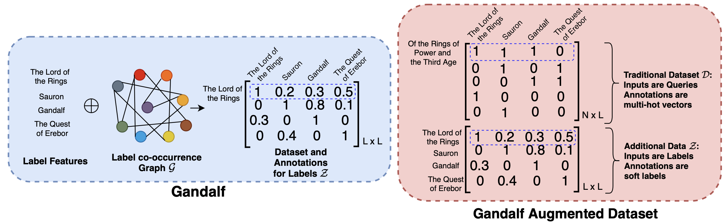
Figure 1. Gandalf augments the training dataset $\mathcal{D}$ by generating soft targets for each label based on label co-occurrence statistics. These additional datapoints $\mathcal{Z}$ are simply concatenated to the traditional dataset for training.

Example 1: For “Mario Kart: Double Dash!!” on Amazon, we have available: Mario Party 7 $|$ Super Smash Bros Melee $|$ Super Mario Sunshine $|$ Super Mario Strikers as the recommended products.

Example 2: For the “2022 French presidential election” Wikipedia page, we have the available categories: April 2022 events in France $|$ 2022 French presidential election $|$ 2022 elections in France $|$ Presidential elections in France. Further, a google search of the same query, leads to the following related searches - French election 2022 - The Economist $|$ French presidential election coverage on FRANCE 24 $|$ Presidential Election 2022: A Euroclash Between a “Liberal… $|$ French polls, trends and election news for France, amongst others.

In view of these examples, one can affirm two important observations: (i) the short-text XMC problem indeed requires recommending similar items which are either highly correlated or co-occur frequently with the queried item, and (ii) the queried item and the corresponding label-features form an “equivalence class” and convey similar intent (Dahiya et al., 2021a). For example, a valid news headline search should either result in a page mentioning the same headline or similar headlines from other media outlets (see Example 2). As a result, it can be argued that data instances are interchangeable with their respective labels’ features.

Exploiting this interchangeability of label and instance text, Dahiya et al. (2021a, 2023) proposes to tie encoder and decoder together and require $\labeldec[l]=\Phi(\labelfeature[l])$. While indeed yielding improved test performance, the condition $\labeldec[l]=\Phi(\labelfeature[l])$ turns out to be too strong, and it has to allow for some fine-tuning corrections $\bm{\eta}_{l}$, yielding $\labeldec[l]=\Phi(\labelfeature[l])+\bm{\eta}_{l}$. Consequently, training of SiameseXML and NGAME is done in two stages: a contrastive loss needs to be minimized, followed by fine-tuning with a classification objective.

Label correlations

Label-label dependencies can appear in multi-label classification in two different forms: Conditional label correlations, and marginal label correlations (Dembczyński et al., 2012). In the conditional case, label dependencies are considered conditioned on each individual query, that is, they are independent if

(2) $$\probability[\mathbf{Y}\mid X]={\textstyle\prod_{j}}\probability[Y_{j}\mid X]\,.$$

As an example, consider the search query “Jaguar”: If we know just this search term, the results pertaining to both, the car brand and the animal, are likely to be relevant. However, knowing that during a particular instance of this search, the user was interested in the animal, one can conclude that car-based labels are less likely to be relevant. In this way, the presence of one label gives information beyond what can be extracted just from the search query.

On the other hand, similar labels will generally appear together. Taking example 2 from the previous section, labels “2022 events in France” and “2022 elections in France” will have an above-random chance of occurring together; however, that information is already carried in the query “2022 French presidential election”, so the presence of one of these labels doesn’t provide any new information, given the query. In that sense, labels are marginally independent if

(3) $$\probability[\mathbf{Y}]={\textstyle\prod_{j}}\probability[Y_{j}]\,.$$

Given an instance, OvA classifiers generate scores independently for all labels. Thus, they are fundamentally incapable of modelling conditional label dependence. However, as standard performance metrics (P@k, PSP@k) are also decomposable into independent contributions of each label, that is, they can be expressed purely in terms of label marginals, they are similarly incapable of detecting whether a classifier models conditional label dependence (Dembczyński et al., 2012).

This means that, as long as we want to focus on these standard metrics (and not on inter-dependency aware losses such as Hüllermeier et al. (2022)), we only need to care about marginal correlations. At first glance, this seems trivial: It can be shown that an OvA classifier, trained using a proper loss, is consistent for P@k (Wydmuch et al., 2018; Menon et al., 2019). Unfortunately, consistency only tells us that, in the limit of infinite training data, we will get a Bayes-optimal classifier. However, in practice, the XMC setting is very far from infinite data—most tail labels will have less than five positive training examples.

Thus, the question we want to tackle here is: Can we exploit knowledge about marginal label correlations to improve training in the data-scarce regime of long-tailed multi-label problems?

3. Gandalf: Learning From Label-Label Correlations

By combining marginal label correlations with label features, we can extend the self-annotation postulate of Dahiya et al. (2021a) to:

Postulate 3.1.

Label-feature Annotation: Given a label $j$ with label-features $\labelfeature[j]$, we posit that if these features are posed as a data point, its labels should follow the marginal label correlations, that is

(4) $$\probability[Y_{i}=1\mid X=\labelfeature[j]]\approx\probability[Y_{i}=1\mid Y_{j}=1]\,.$$

Note that this reduces to self-annotation by setting $i=j$, in which case equation 4 becomes $\probability[Y_{j}\mid\labelfeature[j]]\approx\probability[Y_{j}\mid Y_{j}]=1$.

LF-AmazonTitles-131K LF-WikiSeeAlsoTitles-320K Training Data P@1 P@3 P@5 PSP@1 PSP@3 PSP@5 P@1 P@3 P@5 PSP@1 PSP@3 PSP@5 original $\mathcal{D}$ 35.62 24.13 17.35 27.53 33.06 37.50 21.53 14.19 10.66 13.06 14.87 16.33 surrogate $\mathcal{Z}$ 29.68 21.47 16.04 28.76 33.75 38.27 22.88 16.02 12.44 22.03 23.69 25.55 $\mathcal{G}=\mathcal{Z}\cup\mathcal{D}$ 43.52 29.23 20.92 36.96 42.71 47.64 31.31 21.38 16.22 24.31 26.79 28.83 $\mathcal{U}(\mathcal{G},N)$ 38.46 25.81 18.52 32.29 37.17 41.59 25.93 17.54 13.34 19.75 21.76 23.57 $\mathcal{Z}^{1}\cup\mathcal{D}$ 37.59 25.25 18.18 30.75 35.54 40.06 24.43 16.16 12.15 16.89 18.45 20.02

Table 2. Experiments showing the quality of the datasets created with label features on InceptionXML. While the baseline is surpassed by training on the combined dataset $\mathcal{G}$, it is also beaten by training on $\mathcal{Z}$, where $|\mathcal{Z}|<|\mathcal{N}|/2$, underscoring its quality.

In words, this means that, if the presence of label $j$ indicates that label $i$ would occur with a certain probability for that same instance, then we assume that this probability is also how likely that label $i$ is to be relevant to a data point that consists of the label features of label $j$. The right side of equation 4 can be written as

(5) $$\probability[Y_{i}=1\mid Y_{j}=1]=\probability[Y_{i}=1,Y_{j}=1]/\probability[Y_{j}=1]\,.$$

Thus, we can use the co-occurrence statistics $G_{ij}\coloneqq\probability[Y_{i}=1,Y_{j}=1]$ to calculate the conditionals, and thus apply a plug-in approach using empirical co-occurrence:

$$\probability[Y_{i}=1\mid Y_{j}=1]\approx\frac{\hat{G}_{ij}}{\hat{G}_{jj}}\,,\text{where},\hat{G}_{ij}\coloneqq\sum_{s=1}^{n}y_{si}y_{sj}\,.$$

Of course, in the data-scarce XMC regime, the co-occurrence matrix $\bm{G}$ will be very noisy. In practice, we empirically find it beneficial to threshold the soft labels at $\delta$, so that label features as data-points are annotated by:

(6) $$y_{ij}^{\mathrm{G}}\coloneqq\begin{cases}\hat{G}_{ij}/\hat{G}_{jj}\text{ if }&\hat{G}_{ij}/\hat{G}_{jj}>\delta\\ 0&\text{otherwise}\end{cases}\,.$$

By approximating the left-hand side of equation 4 using a parameterized model $\Psi$, and taking the empirical co-occurrence as a noise estimate for the right-hand side, we can turn this equation into a (surrogate) machine-learning task. This is the same problem as the original XMC task equation 1, applied to a different dataset $\mathcal{Z}=\{(\labelfeature[i],\smash{\labelvec[i]^{\mathrm{G}}})\}_{i=1}^{L}$. That is, we want to optimize

(7) $$\mathcal{L}_{\mathcal{Z}}[\Psi,\labeldec]\coloneqq\sum_{i,j=1}^{L}y_{ij}^{\mathrm{G}},\langle\Psi(\labelfeature[j]),\labeldec[i]\rangle)\,.$$

In Table 2, we present results for training on this surrogate task (row “Training on $\mathcal{Z}$”), when evaluating the resulting classifier on the original test set. The results are striking, and provide a strong confirmation of the equivalence principle between label features and input texts: Even though this model has never seen any actual training instance, it performs adequate (AmazonTitles) or better (WikiSeeAlsoTitles) than the original model in terms of precision at $k$. Looking at PSP, which gives more weight to tail labels, it actually outperforms the original model, in some cases with a large margin.

This tells us that we can, in fact, identify the two encoders in equations 1 and 7, $\Psi\equiv\Phi$, and train a single model on the combined dataset $\mathcal{G}=\mathcal{D}\cup\mathcal{Z}$, as illustrated in Figure 1. This combination of data can yield strong improvements on both regular and propensity scored metrics.

3.1. Bias-Variance Trade-off

This improvement cannot be explained by the increased training set size $|\mathcal{G}|=N+L$ alone, as we can show with the following simple experiment: We generate a new dataset $\mathcal{G}^{\prime}\sim\mathcal{U}(\mathcal{G},N)$ by uniformly sampling (without replacement) from the combined dataset a subset that has the same size as the original training set $|\mathcal{D}|=N$. Table 2 shows that this already leads to significant improvements over the original training set.

To explain this phenomenon, we note that this augmented data is qualitatively slightly different from the original training instances: the empirical co-occurrence matrix $\hat{\bm{G}}$ provides soft labels $\labelvec[i]^{\mathrm{G}}$ as training targets. XMC dataset exhibit high variance (Babbar and Schölkopf, 2019; Anonymous, 2024) because of the long tail labels, whereas the soft labels of the augmented points provide a much smoother training signal. On the other hand, they are based on the approximation of Postulate 3.1, and as such, will introduce some additional bias into the method, essentially leading to a highly favourable bias-variance trade-off.

In fact, the reduction in variance is so helpful to the training process that even switching out equation 4 with one-hot labels based purely on the self-annotation principle ($y_{ij}^{\mathrm{SA}}\coloneqq\indicator[i=j]$ such that $\mathcal{Z}^{1}=\{(\labelfeature[i],\smash{\labelvec[i]^{\mathrm{SA}}})\}_{i=1}^{L}$), thus considerably increasing the bias in the generated data, we still get significant improvements over just using the original training data (Table 2).

3.2. Connection to GLaS regularization

In order to derive a model for $\mathbb{P}[Y_{l^{\prime}}=1\mid X=\labelfeature[l]]$, we can take inspiration from the Glas regularizer (Guo et al., 2019). This regularizer tries to make the Gram matrix of the label embeddings $\langle\labeldec[i],\labeldec[j]\rangle$ reproduce the co-occurrence statistics of the labels $\mathbf{S}$,

(8) $$\mathcal{R}_{\text{GLaS}}[\labeldec]=L^{-2}\sum_{i=1}^{L}\sum_{j=1}^{L}\left(\langle\labeldec[i],\labeldec[j]\rangle-S_{ij}\right)^{2}.$$

Here, $\mathbf{S}$ denotes the symmetrized conditional probabilities,

(9) $$S_{ij} \coloneqq 0.5(\mathbb{P}[Y_{i}=1\mid Y_{j}=1]+\mathbb{P}[Y_{j}=1\mid Y_{i}=1])$$

$$\approx 0.5(\hat{G}_{ij}/\hat{G}_{jj}+\hat{G}_{ij}/\hat{G}_{ii})\,.$$

By the self-proximity postulate (Dahiya et al., 2021a), we can assume $\labeldec[l]\approx\Phi(\labelfeature[l])$. For a given label feature instance with target soft-label $(\labelfeature[l],y^{\text{GLaS}}_{ll^{\prime}})$, the training will try to minimize $\ell(\langle\Phi(\labelfeature[l]),\labeldec[l^{\prime}]\rangle,y^{\text{GLaS}}_{ll^{\prime}})$. To be consistent with Equation 8, we therefore want to choose $y^{\text{GLaS}}_{ll^{\prime}}$ such that $S_{ll^{\prime}}=\operatorname*{arg\,min}\ell(\cdot,y^{\text{GLaS}}_{ll^{\prime}})$. This is fulfilled for $y^{\text{GLaS}}_{ll^{\prime}}=\sigma(S_{ll^{\prime}})$ for $\ell$ being the binary cross-entropy, where $\sigma$ denotes the logistic function.

While the soft targets generated this way slightly differ from the ones of equation 6, as already observed, the bias introduced by mildly incorrect training targets is offset by far by the variance reduction, and we find that this version performs only slightly worse than Gandalf (Appendix A).

4. Experiments

Benchmarks, Baseline and Metrics

We benchmark our experiments on 4 standard public datasets, the details of which are mentioned in Table 1. To test the generality and effectiveness of our proposed Gandalf, we apply the algorithm across a variety of state-of-the-art short-text extreme classifiers. These consist of (i) base frugal models -Astec (Dahiya et al., 2021b) and InceptionXML (Kharbanda et al., 2023) - which do not, by default, leverage label text information, (ii) Decaf (Mittal et al., 2021a), Eclare (Mittal et al., 2021b) and InceptionXML-LF which equip the base models with additional encoders to make use of label text and label correlation information and, (iii) Ngame + Renee - consisting of Renee (Jain et al., 2023), which makes CUDA optimizations to train BCE loss over a classifier for $L$ labels without a shortlist. The transformer encoder is initialized with pre-trained Ngame (M1, dual encoder) (Dahiya et al., 2023). We measure the performance using standard metrics P@k, its propensity-scored variant, PSP@k (Jain et al., 2016; Qaraei et al., 2021), and coverage@k (Schultheis et al., 2022, 2024).

Method P@1 P@3 P@5 PSP@1 PSP@3 PSP@5 P@1 P@3 P@5 PSP@1 PSP@3 PSP@5 LF-AmazonTitles-131K LF-AmazonTitles-1.3M SiameseXML 41.42 30.19 21.21 35.80 40.96 46.19 49.02 42.72 38.52 27.12 30.43 32.52 Astec 37.12 25.20 18.24 29.22 34.64 39.49 48.82 42.62 38.44 21.47 25.41 27.86 + Gandalf 43.95 29.66 21.39 37.40 43.03 48.31 53.02 46.13 41.37 27.32 31.20 33.34 Decaf 38.40 25.84 18.65 30.85 36.44 41.42 50.67 44.49 40.35 22.07 26.54 29.30 + Gandalf 42.43 28.96 20.90 35.22 42.12 47.61 53.02 46.65 42.25 25.47 30.14 32.83 Eclare 40.46 27.54 19.63 33.18 39.55 44.10 50.14 44.09 40.00 23.43 27.90 30.56 + Gandalf 42.51 28.89 20.81 35.72 42.19 47.46 53.87 47.45 43.00 28.86 32.90 35.20 InceptionXML 36.79 24.94 17.95 28.50 34.15 38.79 48.21 42.47 38.59 20.72 24.94 27.52 + Gandalf 44.67 30.00 21.50 37.98 43.83 48.93 50.80 44.54 40.25 25.49 29.42 31.59 InceptionXML-LF 40.74 27.24 19.57 34.52 39.40 44.13 49.01 42.97 39.46 24.56 28.37 31.67 + Gandalf 43.84 29.59 21.30 38.22 43.90 49.03 52.91 47.23 42.84 30.02 33.18 35.56 Ngame + Renee 46.05 30.81 22.04 38.47 44.87 50.33 56.04 49.91 45.32 28.54 33.38 36.14 + Gandalf 45.86 30.53 21.79 40.49 45.83 50.96 56.88 50.24 45.47 26.56 31.69 34.60 LF-WikiSeeAlsoTitles-320K LF-WikiTitles-500K SiameseXML 31.97 21.43 16.24 26.82 28.42 30.36 42.08 22.80 16.01 23.53 21.64 21.41 Astec 22.72 15.12 11.43 13.69 15.81 17.50 44.40 24.69 17.49 18.31 18.25 18.56 + Gandalf 31.10 21.54 16.53 23.60 26.48 28.80 45.24 25.45 18.57 21.72 20.99 21.16 Decaf 25.14 16.90 12.86 16.73 18.99 21.01 44.21 24.64 17.36 19.29 19.82 19.96 + Gandalf 31.10 21.60 16.31 24.83 27.18 29.29 45.27 25.09 17.67 22.51 21.63 21.43 Eclare 29.35 19.83 15.05 22.01 24.23 26.27 44.36 24.29 16.91 21.58 20.39 19.84 + Gandalf 31.33 21.40 16.31 24.83 27.18 29.29 45.12 24.45 17.05 24.22 21.41 20.55 InceptionXML 23.10 15.54 11.52 14.15 16.71 17.39 44.61 24.79 19.52 18.65 18.70 18.94 + Gandalf 32.54 22.15 16.86 25.27 27.76 30.03 45.93 25.81 20.36 21.89 21.54 22.56 InceptionXML-LF 28.99 19.53 14.79 21.45 23.65 25.65 44.89 25.71 18.23 23.88 22.58 22.50 + Gandalf 33.12 22.70 17.29 26.68 29.03 31.27 47.13 26.87 19.03 24.12 23.92 23.82 Ngame + Renee 30.79 20.65 15.57 20.81 24.46 27.05 - - - - - - + Gandalf 33.92 23.11 17.58 24.15 26.23 30.89 - - - - - -

Table 3. Results showing the effectiveness of Gandalf on state-of-the-art extreme classifiers. The best results are in bold.

4.1. Main Results

Gandalf vs Architectural Additions (LTE, GALE)

The first formal attempt to externally imbue the model with label information was made with Decaf, which essentially equips the base model Astec with another base encoder (LTE) to learn label text ($\labelfeature[l]$) embeddings along with the classifier. The second attempt, in the form of Eclare, builds upon Decaf by adding another base encoder (GALE) to process and externally capture label correlation information. To make our claim more general, we also evaluate on InceptionXML-LF, which consist of the same extensions on a more recent base model InceptionXML (Kharbanda et al., 2023) with LTE and GALE components (just as Eclare adds LTE and GALE to Astec). While such architectural modifications help capture higher order query-label relations and increase empirical performance, they also increase both training time and the peak GPU memory required during training by $\sim 3\times$.

As Gandalf is a data-centric approach, the memory overhead is eliminated by default. Further, we find that (i) Decaf and Eclare still benefit from using Gandalf augmented data implying architectural modifications are complementary to Gandalf. However, (ii) simply using Gandalf augmented data enables base models Astec and InceptionXML outperform themselves by up to 30% and perform nearly at par with their more architecturally equipped counter parts Eclare and InceptionXML-LF. While we posit that Gandalf and GALE learn complementary data relations, both our quantitative (Table 3) and qualitative (Table 4, Figure 2) results show that Gandalf is more effective and efficient at capturing these relations (specifically, label correlations) compared to the latter.

Gandalf vs Siamese Learning

Consequently, the third attempt made at capturing label correlations via SiameseXML, which essentially replaces the surrogate training task in Astec with a two-tower siamese learning framework. As argued in section 2, the condition $\labeldec[l]=\Phi(\labelfeature[l])$ turns out to be too strong, and consequently training of SiameseXML and NGAME is done in two stages. Initially, a contrastive loss needs to be minimized, followed by fine-tuning with a classification objective which allows for some fine-tuning corrections $\bm{\eta}_{l}$, yielding $\labeldec[l]=\Phi(\labelfeature[l])+\bm{\eta}_{l}$. On the other hand, Gandalf simply extends training data to learn from a-priori label co-occurrence data in a supervised manner. Notably (from Table 3), Astec + Gandalf outperforms SiameseXML by 5-10% on Amazon datasets, while performing at par on Wikipedia datasets.

Applying Gandalf to Two-tower approaches

Although we propose Gandalf as a method suitable for training classifiers, it can also be used leveraged alongside two-tower approaches, like Ngame. This is done by first extending the dual encoder with a scalable classifier with Renee, which simply trains OvA classifiers on top of the base model. Using Gandalf augmented data during this extension leads to significant improvements, more prominently on the LF-WikiSeeAlsoTitles-320K and LF-AmazonTitles-131K datasets.

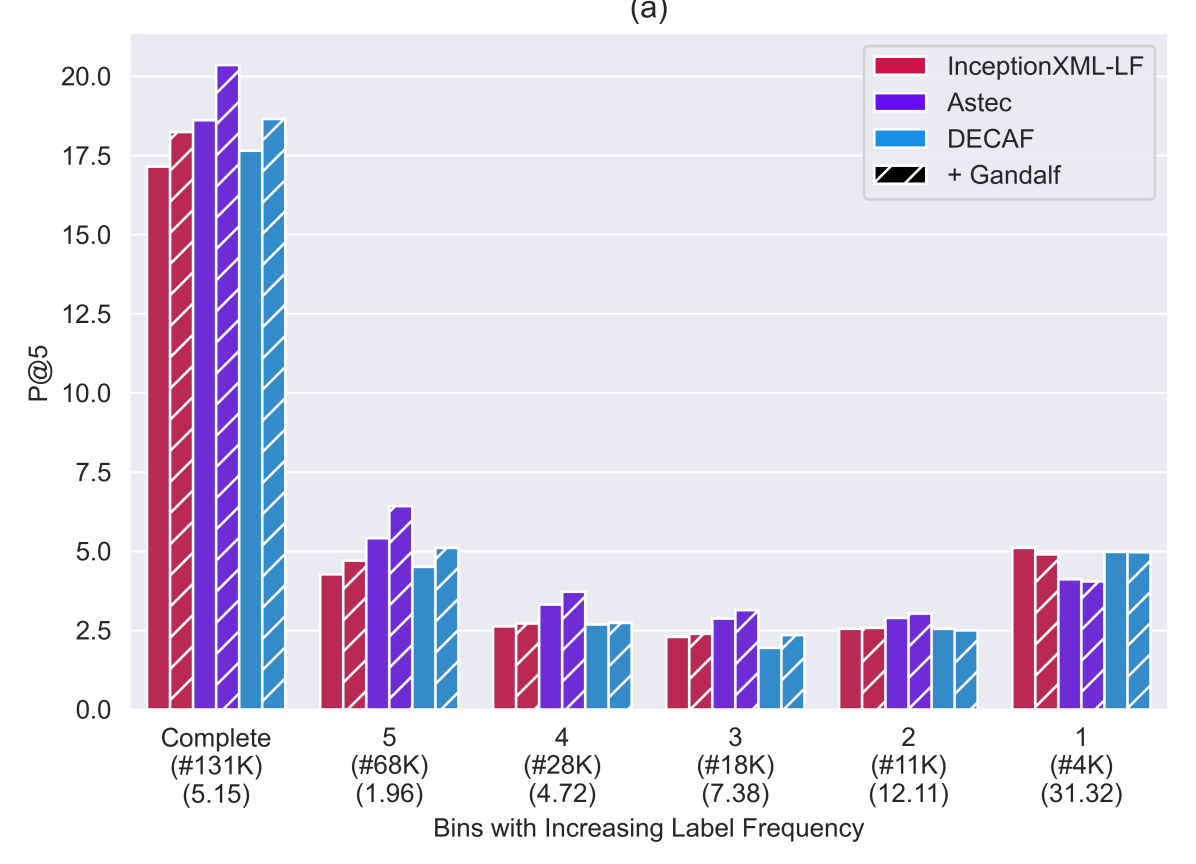
Figure 2. Gandalf demonstrating improvements on the P@5 metric across various methods, separated into tail, torso and head lables. On the x axis, the middle row indicates the number of labels in the bin, and the lowest row denotes the average number of positives per label in that bin. Improvements in earlier bins (5 - 3) denote gains in tail label performance.

Improvements on tail labels

We perform a quantile analysis across 2 datasets – LF-AmazonTitles-131K (Figure 2) and the LF-WikiSeeAlsoTitles-320K (Figure 4, Appendix A) with InceptionXML – where we examine performance (contribution to P@5 metric) over 5 equi-voluminous bins based on increasing order of mean label frequency in the training dataset. Consequently, performance on head labels can be captured by the bin #1 and that of tail labels by bin #5. We note that introducing the additional training data with Gandalf consistently improves the performance across all label frequencies, with more profound gains on bins with more tail labels. This is further verified by significant performance boosts, with base models showing upto 11% improvements in the PSP@k metrics in Table 3.

Beyond model performances

We can also extract dataset specific insights with Gandalf from Table 3. Significant improvements on top of the base algorithm are particularly observed on LF-AmazonTitles-131K and LF-WikiSeeAlsoTitles-320K. In contrast, improvements on LF-WikiTitles-500K remain relatively mild. We attribute this to the density of the datasets. Specifically, while the former datasets consist of $\sim$5 training instances per label, the latter consists of $\sim$17. We posit a higher query-label density enables algorithms to inherently learn sufficient label-label correlations from existing data. However, we further see that using Gandalf is effective for LF-AmazonTitles-1.3M, the largest public benchmark for XMC with label features. Here, even though average training instances per label is $\sim$38, the average number of labels per instance is $\sim$22, as compared to maximum of $\sim$4 on other datasets.

Qualitative Results

We further analyse qualitative examples via the top 5 predictions obtained by training the base encoders with and without Gandalf augmented data points in Table 4, with more examples in Appendix A. Notably, we can observe that queries with even a single keyword (Oat), which have no correct predictions without Gandalf, result in 100% correct predictions with it. Furthermore, even the quality of incorrect predictions improves . For example, in case of “Lunar Orbiter program”, the only incorrect Gandalf predictions are “Lunar Orbiter 3”, “Lunar Orbiter 5” and “Pioneer program” (US lunar and planetary space programs).

Additionally, we show semantic similarity between the annotated labels with $\mathcal{G}$, and the original label in Figure 5 in Appendix A.

Method Datapoint Baseline Predictions Gandalf Predictions InceptionXML-LF Pontryagin duality, Topological order, Topological quantum field theory, Topological quantum number, Quantum topology Compact group, Haar measure, Lie group, Algebraic group, Topological ring Decaf Topological group Topological quantum computer, Topological order, Topological quantum field theory, Topological quantum number, Quantum topology Compact group, Haar measure, Lie group, Algebraic group, Topological ring Eclare Topological quantum computer, Topological order, Topological quantum field theory, Topological quantum number, Quantum topology Compact group, Topological order, Lie group, Algebraic group, Topological ring InceptionXML-LF List of lighthouses in Scotland, List of Northern Lighthouse Board lighthouses, Oatcake, Communes of the Finistere department, Oat milk Oatcake, Oatmeal, Oat milk, Porridge, Rolled oats Decaf Oat Oatcake, Oatmeal, Design for All (in ICT), Oatley Point Reserve, Oatley Pleasure Grounds Oatcake, Oatmeal, Oat milk, Porridge, Rolled oats Eclare Oatmeal, Oat milk, Parks in Sydney, Oatley Point Reserve, Oatley Pleasure Grounds Oatcake, Porridge, Rolled oats, Oatley Point Reserve, Oatley Pleasure Grounds InceptionXML-LF Lunar Orbiter Image Recovery Project, Lunar Orbiter 3, Lunar Orbiter 5, Chinese Lunar Exploration Program, List of future lunar missions Surveyor program, Luna programme, Lunar Orbiter Image Recovery Project, Lunar Orbiter 3, Lunar Orbiter 5 Decaf Lunar Orbiter program Exploration of the Moon, List of man-made objects on the Moon, Lunar Orbiter Image Recovery Project, Lunar Orbiter 3, Lunar Orbiter 5 Exploration of the Moon, Apollo program, Surveyor program, Luna programme, Lunar Orbiter program Eclare Exploration of the Moon, Lunar Orbiter program, Lunar Orbiter Image Recovery Project, Lunar Orbiter 3, Lunar Orbiter 5 Exploration of the Moon, Pioneer program, Surveyor program, Luna programme, Lunar Orbiter program InceptionXML-LF Colorado metropolitan areas, Front Range Urban Corridor, Outline of Colorado, Index of Colorado-related articles, State of Colorado Colorado metropolitan areas, Outline of Colorado, Index of Colorado-related articles, Colorado cities and towns, Colorado counties Decaf Grand Lake, Colorado Colorado metropolitan areas, Front Range Urban Corridor, State of Colorado, Colorado municipalities, National Register of Historic Places listings in Grand County, Colorado Outline of Colorado, State of Colorado, Colorado cities and towns, Colorado municipalities, Colorado counties Eclare State of Colorado, Colorado cities and towns, Colorado counties, National Register of Historic Places listings in Grand County, Colorado, Grand County, Colorado Outline of Colorado, Index of Colorado-related articles, State of Colorado, Colorado cities and towns, Colorado counties

Table 4. Qualitative predictions from the LF-WikiSeeAlsoTitles-320K dataset. Labels indicate mispredictions.

4.2. Ablation & Computational Analysis

Gandalf, is a data-centric approach that does not increase the computational cost during inference. While the inclusion of label features - which can often run in the order of millions - as additional data points might seem to increase the computational cost during training, through a series of observations, we show that this is in fact not the case. On the contrary, Gandalf can help in reducing the memory footprint while training, enabling researchers to use smaller GPUs, and reallocating their compute budget towards longer training schedules. Secondly, we also study the effect of subsampling the labels used for Gandalf to demonstrate how learning even some of the label-label correlations is beneficial for XMC models. This observation is particularly useful when inclusion of all label-features as data points becomes intractable due to its scale.

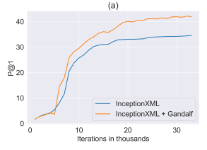
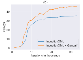
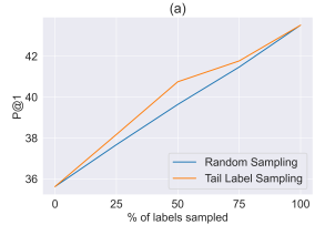
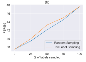
Figure 3. The (a) P@1 and (b) PSP@5 metric plotted against iterations for InceptionXML with and without Gandalf. The effect of subsampling labels for Gandalf on the (c) P@1 and (d) PSP@5 metric. Both results are on the LF-AmazonTitles-131K dataset.

Method P@1 P@3 P@5 PSP@1 PSP@3 PSP@5 P@1 P@3 P@5 PSP@1 PSP@3 PSP@5 LF-AmazonTitles-131K LF-WikiSeeAlsoTitles-320K InceptionXML 35.62 24.13 17.35 27.53 33.06 37.50 21.53 14.19 10.66 13.06 14.87 16.33 + Gandalf $\mathcal{G}$ 43.71 29.30 21.14 37.25 43.01 47.89 31.42 21.54 16.37 24.78 27.36 28.98 + Gandalf ($\mathcal{G}$ + Random Walk (Mittal et al., 2021b)) 43.52 29.23 20.92 36.96 42.71 47.64 31.31 21.38 16.22 24.31 26.79 28.83 InceptionXML-LF 40.74 27.24 19.57 34.52 39.40 44.13 49.01 42.97 39.46 24.56 28.37 31.67 + Gandalf ($\delta$ = 0.0) 41.71 28.03 20.14 36.94 41.93 46.64 31.40 21.56 16.53 26.01 27.89 29.99 + Gandalf ($\delta$ = 0.1) 42.09 28.38 20.45 37.09 42.19 47.04 32.20 21.86 16.60 26.06 28.01 30.03 + Gandalf ($\delta$ = 0.2) 41.73 28.10 20.18 37.01 41.99 46.67 31.29 21.35 16.28 25.68 27.59 29.65

Table 5. Results demonstrating the effectiveness of Gandalf using both, a statistical co-occurrence matrix ($\mathcal{G}$) and it’s modified version using a random walk as in (Mittal et al., 2021b). The table also shows the method’s sensitivity to $\delta$, as defined in Equation 6.

Computational Costs during Training

For the LF-Amazon- Titles-131K dataset, we plot the P@1 and the PSP@5 metric against iterations for InceptionXML, trained with and without Gandalf in Figure 3. As can be seen, using Gandalf gives better performance, even on tail labels, right from the beginning. Moreover, where the performance of InceptionXML saturates, the performance of Gandalf continues to scale with increasing compute. Therefore, given a fixed computational budget, a model trained with Gandalf will outperform one trained without it. This can also be seen in Table 2 where training on $\mathcal{U}(\mathcal{G},N)$, i.e., under the exact same computational budget as training on the the original dataset gives performance improvements. In the same table, we can also observe improvements when training on less than half the original compute with $\mathcal{Z}$ . These observations firmly place Gandalf as a compute-efficient method of leveraging label-features in XMC models.

Effect of Subsampling Labels

We demonstrate the effect of subsampling labels used for Gandalf under two schemes, (a) Randomly sampling an expected percentage subset of labels and (b) randomly sampling this subset from equi-voluminous bins of increasing label frequency, i.e., prioritising tail labels for lower percentages. These results are shown for the P@1 and PSP@5 metric on the LF-AmazonTitles-131K dataset in Figure 3.

Both the metrics grow linearly as the percentage sampled labels are increased in steps of 25%. This goes ahead to show the lack of label-label correlations being captured in existing methods, and how learning even on a subset can be useful. Further, prioritising tail-labels consistently outperforms the random sampling baseline, underscoring the data-scarcity issue in XMC.

Choice of label co-occurrence graph $\mathcal{G}$

While with Gandalf, we leverage a statistical measure for $\mathcal{G}$, we can also estimate it with random walks (Mittal et al., 2021b) (used for GALE). We find that our method is not significantly affected by this choice, with the co-occurrence graph giving slightly enhanced performance(Table 5). We hypothesise this happens due to the noise introduced via random walks. While both variants aim to model similar information, their differing usage determines their overall effectiveness. In particular, leveraging it for Gandalf helps learn sufficient information on top of GALE.

Sensitivity to $\delta$

We examine Gandalf’s sensitivity to $\delta$ by training InceptionXML-LF on data generated with varying values of $\delta$. As shown in Table 5, the empirical performance peaks at a $\delta$ value of $0.1$ which is sufficient to suppresses the impact of noisy correlations. Higher values of $\delta$ tend to suppress useful information.

5. Other Related Work

Prior works in XMC focused on annotating long-text documents, consisting of hundreds of word tokens, such as those encountered in tagging for Wikipedia (Babbar and Schölkopf, 2017; Khandagale et al., 2020; You et al., 2019; Schultheis and Babbar, 2022) with numeric label IDs. Most recent works under this setting were aimed towards scaling up transformer encoders for the XMC task (Zhang et al., 2021a; Kharbanda et al., 2022).

Exploiting Correlations in XMC

For XMC datasets endowed with label features, there exist three correlations that can be exploited for better representation learning : (i) query-label, (ii) query-query, and (iii) label-label correlations. Recent works have been successful in leveraging label features and pushing state-of-the-art by exploiting the first two correlations. For example, SiameseXML and NGAME (Dahiya et al., 2021a, 2023) employ a two-tower pre-training stage applying contrastive learning between an input text and its corresponding label features. GalaXC (Saini et al., 2021) & PINA (Chien et al., 2023), motivated by graph convolutional networks, create a combined query-label bipartite graph to aggregate predicted instance neighbourhood. This approach, however, leads to a multifold increase in the memory footprint. Decaf and Eclare (Mittal et al., 2021a, b) make architectural additions to embed label-text embeddings (LTE) and graph-augmented label embeddings (GALE) in each label’s OVA classifier to exploit higher order correlations from the random walk graph. PINA, in its pre-training step, leverages label features as data points, but does so by expanding the label space $\{0,1\}^{L}$ to also include instances as $\{0,1\}^{L+N}$ leveraging the self-annotation property of labels (Dahiya et al., 2021a) and inverting the initial instance-label mappings to have instances $\instance[i]$ as labels for label features $\labelfeature[l]$ as data points. This, however, leads to an explosion in an already enormous label space. In this work, we find that a significant amount of information can be learned by modelling label-label correlations, which existing methods fail to leverage.

Two-tower Models & Classifier Learning

Typically, due to the single-annotation nature of most dense retrieval datasets (Nguyen et al., 2016; Kwiatkowski et al., 2019; Joshi et al., 2017), two-tower models (Karpukhin et al., 2020) solving this task eliminate classifiers in favour of modelling implicit correlations by bringing query-document embeddings closer in the latent space of the encoders. These works are conventionally aimed at improving encoder representations by innovating on hard-negative mining (Zhang et al., 2021b; Xiong et al., 2021; Lu et al., 2022), teacher-model distillation (Qu et al., 2021; Ren et al., 2021) and combined dense-sparse training strategies (Khattab and Zaharia, 2020). While these approaches result in enhanced encoders, the multilabel nature of XMC makes them, in itself, insufficient for this domain. This has been demonstrated in two-stage XMC works like Dahiya et al. (2021a, 2023); Jain et al. (2023) where these frameworks go beyond two-tower training and train classifiers with a frozen encoder in the second stage for better empirical performance. While a concurrent work (Gupta et al., 2023) does show that dual-encoder XMC models can outperform classifiers, but requires significant computational resources to scale the contrastive loss across the entire label space.

6. Conclusion

In this paper, we proposed Gandalf, a strategy to learn label correlations, a notoriously difficult challenge. In contrast to previous works which model these correlations implicitly through model training, we propose a supervised approach to explicitly learn them by leveraging the inherent query-label symmetry in short-text extreme classification. We further performed extensive experimentation by implementing on various SOTA XMC methods and demonstrated dramatic increases in prediction performances uniformly across all methods. Moreover, this is achieved with frugal architectures without incurring any computational overheads in inference latency or training memory footprint. We hope our treatment of label correlations in this domain will spur further research towards crafting data-points with more expressive annotations, and further extend it to long-text XMC approaches where the instance-label symmetry is quite ambiguous.

Appendix A Additional Visualizations

Additional Qualitative Examples

The same observations in the examples provided in the main paper can be made for these additional examples as well (Table 4). Where initially we mispredict all the labels, with Gandalf, we can correctly predict all the labels.

Similarity between Labels and their Annotations

Each label and their annotations, as discovered by the co-occurrence graph, are semantically similar; in that they share tokens with one another and can be used in the same context. We show this pictorially by plotting the labels and their annotations in order of their co-occurrence in Figure 5.

Additional Quantile Analysis for Tail Labels

We show an additional quantile analysis on the LF-WikiSeeAlsoTitles-320K dataset in Figure 4, to demonstrate improvements in labels with different frequencies. The observations remain consistent with that of LF-AmazonTitles-131K in the main paper.

Figure 4. Contributions to P@5 in LF-WikiSeeAlsoTitles-320K. The number of labels in each bin is provided after the # in the second row of the tags on the x-axis. The bottomost row denotes the mean label frequency in that bin. Specifically, note the improvements on tail labels in the earlier bins (5 - 3).

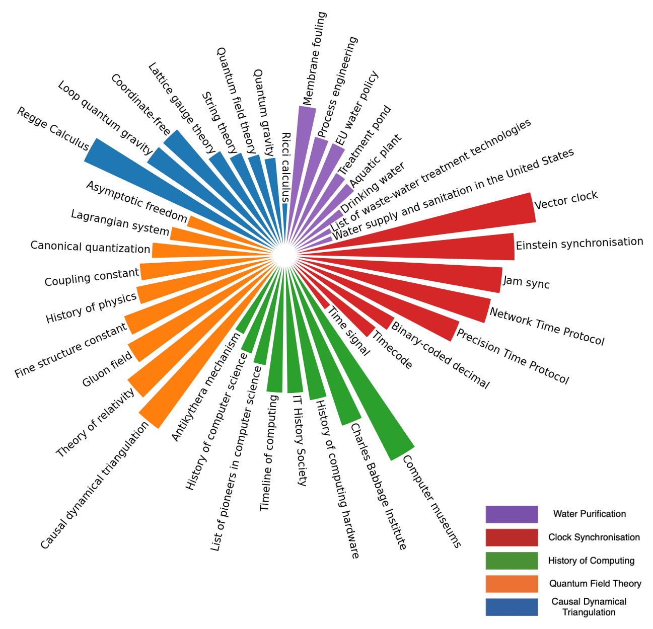
Figure 5. Correlations between labels and their first-order neighbours, as found by the label co-occurrence on the LF-WikiTitles-500K dataset. The legend shows the label in question, the bar chart shows the degree of correlation with its neighbouring labels. Correlated labels often share tokens with each other and/or may be used in the same context.

Appendix B Additional Experiments

Coverage Results

Coverage is an important metric in XMC as it demonstrates the ability of the model to predict tail labels effectively. We provide coverage results on InceptionXML in Table 6, demonstrating that Gandalf learns to predict labels which were previously not being predicted at all. This phenomenon can also be seen in the qualitative results Table 4

Comparison against conventional data augmentation strategies

We compare Gandalf with with existing data augmentation techniques in Table 7. While no such techniques exist specifically for XMC, we use three baselines: synonym replacement(randomly replacing words in the input text with their synonyms, chosen via BERT similarity), MixUp and Label-MixUp. While the first two are standard data augmentations in NLP, Label-Mixup is a modified version of MixUp that combines the feature of a label feature and input datapoint, which is more suitable for XMC. Notably, Gandalf outperforms all of them with a significant margin:

Method C@1 C@3 C@5 C@1 C@3 C@5 LF-AmazonTitles-131K LF-WikiSeeAlsoTitles-320K InceptionXML 22.33 39.98 46.29 7.54 15.11 18.93 + Gandalf 31.04 51.63 58.03 13.28 26.01 32.21

Table 6. Coverage Results on InceptionXML and Gandalf. Best scores are in bold.

Method P@1 P@3 P@5 PSP@1 PSP@3 PSP@5 LF-AmazonTitles-131K InceptionXML 35.62 24.13 17.35 27.53 33.06 37.50 + Synonym Replacement 35.07 23.71 17.08 27.20 32.41 36.77 + MixUp 35.63 24.15 17.37 27.55 33.00 37.63 + Label-MixUp 37.25 25.02 17.98 29.25 34.58 39.09 + Gandalf 43.52 29.23 20.92 36.96 42.71 47.64 LF-WikiSeeAlsoTitles-320K InceptionXML 21.53 14.19 10.66 13.06 14.87 16.33 + Synonym Replacement 20.08 13.13 9.92 12.00 13.50 14.90 + MixUp 21.62 14.15 10.65 13.13 14.99 16.36 + Label-MixUp 23.90 16.10 12.28 15.20 17.60 19.56 + Gandalf 31.31 21.38 16.22 24.31 26.79 28.83

Table 7. Comparison of conventional data augmentation strategies with the proposed Gandalf method. Best scores are in bold.

References

- (1)
- Adamic and Huberman (2002) Lada A Adamic and Bernardo A Huberman. 2002. Zipf’s law and the Internet. Glottometrics 3, 1 (2002), 143–150.
- Anonymous (2024) Anonymous. 2024. Enhancing Tail Performance in Extreme Classifiers by Label Variance Reduction. In The Twelfth International Conference on Learning Representations. https://openreview.net/forum?id=6ARlSgun7J
- Babbar and Schölkopf (2017) R. Babbar and B. Schölkopf. 2017. DiSMEC: Distributed Sparse Machines for Extreme Multi-label Classification. In WSDM.
- Babbar and Schölkopf (2019) R. Babbar and B. Schölkopf. 2019. Data scarcity, robustness and extreme multi-label classification. Machine Learning 108 (2019), 1329–1351.
- Chiang et al. (2019) Wei-Lin Chiang, Xuanqing Liu, Si Si, Yang Li, Samy Bengio, and Cho-Jui Hsieh. 2019. Cluster-GCN: An Efficient Algorithm for Training Deep and Large Graph Convolutional Networks. In Proceedings of the 25th ACM SIGKDD International Conference on Knowledge Discovery & Data Mining (Anchorage, AK, USA) (KDD ’19). Association for Computing Machinery, New York, NY, USA, 257–266. https://doi.org/10.1145/3292500.3330925
- Chien et al. (2023) Eli Chien, Jiong Zhang, Cho-Jui Hsieh, Jyun-Yu Jiang, Wei-Cheng Chang, Olgica Milenkovic, and Hsiang-Fu Yu. 2023. PINA: Leveraging Side Information in eXtreme Multi-label Classification via Predicted Instance Neighborhood Aggregation. arXiv preprint arXiv:2305.12349 (2023).
- Dahiya et al. (2021a) Kunal Dahiya, Ananye Agarwal, Deepak Saini, Gururaj K, Jian Jiao, Amit Singh, Sumeet Agarwal, Purushottam Kar, and Manik Varma. 2021a. SiameseXML: Siamese Networks meet Extreme Classifiers with 100M Labels. In Proceedings of the 38th International Conference on Machine Learning (Proceedings of Machine Learning Research, Vol. 139). PMLR, 2330–2340. https://proceedings.mlr.press/v139/dahiya21a.html
- Dahiya et al. (2023) Kunal Dahiya, Nilesh Gupta, Deepak Saini, Akshay Soni, Yajun Wang, Kushal Dave, Jian Jiao, Gururaj K, Prasenjit Dey, Amit Singh, et al. 2023. NGAME: Negative Mining-aware Mini-batching for Extreme Classification. In Proceedings of the Sixteenth ACM International Conference on Web Search and Data Mining. 258–266.
- Dahiya et al. (2021b) Kunal Dahiya, Deepak Saini, Anshul Mittal, Ankush Shaw, Kushal Dave, Akshay Soni, Himanshu Jain, Sumeet Agarwal, and Manik Varma. 2021b. DeepXML: A Deep Extreme Multi-Label Learning Framework Applied to Short Text Documents. In Proceedings of the 14th ACM International Conference on Web Search and Data Mining (Virtual Event, Israel) (WSDM ’21). Association for Computing Machinery, New York, NY, USA, 31–39. https://doi.org/10.1145/3437963.3441810
- Dembczyński et al. (2012) Krzysztof Dembczyński, Willem Waegeman, Weiwei Cheng, and Eyke Hüllermeier. 2012. On label dependence and loss minimization in multi-label classification. Machine Learning 88 (2012), 5–45.
- Guo et al. (2019) C. Guo, A. Mousavi, X. Wu, Daniel N. Holtmann-Rice, S. Kale, S. Reddi, and S. Kumar. 2019. Breaking the Glass Ceiling for Embedding-Based Classifiers for Large Output Spaces. In NeurIPS.
- Gupta et al. (2023) Nilesh Gupta, Devvrit Khatri, Ankit S Rawat, Srinadh Bhojanapalli, Prateek Jain, and Inderjit S Dhillon. 2023. Efficacy of Dual-Encoders for Extreme Multi-Label Classification. arXiv:2310.10636 [cs.LG]
- Hu et al. (2020) Weihua Hu, Matthias Fey, Marinka Zitnik, Yuxiao Dong, Hongyu Ren, Bowen Liu, Michele Catasta, and Jure Leskovec. 2020. Open Graph Benchmark: Datasets for Machine Learning on Graphs. In Proceedings of the 34th International Conference on Neural Information Processing Systems (Vancouver, BC, Canada) (NIPS’20). Curran Associates Inc., Red Hook, NY, USA, Article 1855, 16 pages.
- Hüllermeier et al. (2022) Eyke Hüllermeier, Marcel Wever, Eneldo Loza Mencia, Johannes Fürnkranz, and Michael Rapp. 2022. A flexible class of dependence-aware multi-label loss functions. Machine Learning 111, 2 (2022), 713–737.
- Jain et al. (2019) Himanshu Jain, Venkatesh Balasubramanian, Bhanu Chunduri, and Manik Varma. 2019. Slice: Scalable Linear Extreme Classifiers Trained on 100 Million Labels for Related Searches. Proceedings of the Twelfth ACM International Conference on Web Search and Data Mining (2019).
- Jain et al. (2016) Himanshu Jain, Yashoteja Prabhu, and Manik Varma. 2016. Extreme multi-label loss functions for recommendation, tagging, ranking & other missing label applications. In KDD. 935–944.
- Jain et al. (2023) Vidit Jain, Jatin Prakash, Deepak Saini, Jian Jiao, Ramachandran Ramjee, and Manik Varma. 2023. Renee: End-to-end training of extreme classification models. Proceedings of Machine Learning and Systems (2023).
- Joshi et al. (2017) Mandar Joshi, Eunsol Choi, Daniel Weld, and Luke Zettlemoyer. 2017. TriviaQA: A Large Scale Distantly Supervised Challenge Dataset for Reading Comprehension. In Proceedings of the 55th Annual Meeting of the Association for Computational Linguistics (Volume 1: Long Papers). Association for Computational Linguistics, Vancouver, Canada, 1601–1611. https://doi.org/10.18653/v1/P17-1147
- Karpukhin et al. (2020) Vladimir Karpukhin, Barlas Oğuz, Sewon Min, Patrick Lewis, Ledell Wu, Sergey Edunov, Danqi Chen, and Wen-tau Yih. 2020. Dense passage retrieval for open-domain question answering. arXiv preprint arXiv:2004.04906 (2020).
- Khandagale et al. (2020) S. Khandagale, H. Xiao, and R. Babbar. 2020. Bonsai: diverse and shallow trees for extreme multi-label classification. Machine Learning 109, 11 (2020), 2099–2119.
- Kharbanda et al. (2023) Siddhant Kharbanda, Atmadeep Banerjee, Devaansh Gupta, Akash Palrecha, and Rohit Babbar. 2023. InceptionXML: A Lightweight Framework with Synchronized Negative Sampling for Short Text Extreme Classification. In Proceedings of the 46th International ACM SIGIR Conference on Research and Development in Information Retrieval (Taipei, Taiwan) (SIGIR ’23). Association for Computing Machinery, Taipei, Taiwan, 760–769. https://doi.org/10.1145/3539618.3591699
- Kharbanda et al. (2022) Siddhant Kharbanda, Atmadeep Banerjee, Erik Schultheis, and Rohit Babbar. 2022. CascadeXML: Rethinking Transformers for End-to-end Multi-resolution Training in Extreme Multi-label Classification. In Advances in Neural Information Processing Systems, Vol. 35. Curran Associates, Inc., 2074–2087. https://proceedings.neurips.cc/paper_files/paper/2022/file/0e0157ce5ea15831072be4744cbd5334-Paper-Conference.pdf
- Khattab and Zaharia (2020) Omar Khattab and Matei Zaharia. 2020. Colbert: Efficient and effective passage search via contextualized late interaction over bert. In Proceedings of the 43rd International ACM SIGIR conference on research and development in Information Retrieval. 39–48.
- Kwiatkowski et al. (2019) Tom Kwiatkowski, Jennimaria Palomaki, Olivia Redfield, Michael Collins, Ankur Parikh, Chris Alberti, Danielle Epstein, Illia Polosukhin, Jacob Devlin, Kenton Lee, Kristina Toutanova, Llion Jones, Matthew Kelcey, Ming-Wei Chang, Andrew M. Dai, Jakob Uszkoreit, Quoc Le, and Slav Petrov. 2019. Natural Questions: A Benchmark for Question Answering Research. Transactions of the Association for Computational Linguistics 7 (2019), 452–466. https://doi.org/10.1162/tacl_a_00276
- Lu et al. (2022) Yuxiang Lu, Yiding Liu, Jiaxiang Liu, Yunsheng Shi, Zhengjie Huang, Shikun Feng Yu Sun, Hao Tian, Hua Wu, Shuaiqiang Wang, Dawei Yin, et al. 2022. Ernie-search: Bridging cross-encoder with dual-encoder via self on-the-fly distillation for dense passage retrieval. arXiv preprint arXiv:2205.09153 (2022).
- Menon et al. (2019) Aditya K Menon, Ankit Singh Rawat, Sashank Reddi, and Sanjiv Kumar. 2019. Multilabel reductions: what is my loss optimising?. In Advances in Neural Information Processing Systems, H. Wallach, H. Larochelle, A. Beygelzimer, F. d'Alché-Buc, E. Fox, and R. Garnett (Eds.), Vol. 32. Curran Associates, Inc. https://proceedings.neurips.cc/paper_files/paper/2019/file/da647c549dde572c2c5edc4f5bef039c-Paper.pdf
- Mittal et al. (2021a) Anshul Mittal, Kunal Dahiya, Sheshansh Agrawal, Deepak Saini, Sumeet Agarwal, Purushottam Kar, and Manik Varma. 2021a. DECAF: Deep Extreme Classification with Label Features. In Proceedings of the 14th ACM International Conference on Web Search and Data Mining (Virtual Event, Israel) (WSDM ’21). Association for Computing Machinery, New York, NY, USA, 49–57. https://doi.org/10.1145/3437963.3441807
- Mittal et al. (2021b) Anshul Mittal, Noveen Sachdeva, Sheshansh Agrawal, Sumeet Agarwal, Purushottam Kar, and Manik Varma. 2021b. ECLARE: Extreme Classification with Label Graph Correlations. In Proceedings of the Web Conference 2021 (Ljubljana, Slovenia) (WWW ’21). Association for Computing Machinery, New York, NY, USA, 3721–3732. https://doi.org/10.1145/3442381.3449815
- Nguyen et al. (2016) Tri Nguyen, Mir Rosenberg, Xia Song, Jianfeng Gao, Saurabh Tiwary, Rangan Majumder, and Li Deng. 2016. Ms marco: A human-generated machine reading comprehension dataset. (2016).
- Partalas et al. (2015) Ioannis Partalas, Aris Kosmopoulos, Nicolas Baskiotis, Thierry Artieres, George Paliouras, Eric Gaussier, Ion Androutsopoulos, Massih-Reza Amini, and Patrick Galinari. 2015. Lshtc: A benchmark for large-scale text classification. arXiv preprint arXiv:1503.08581 (2015).
- Prabhu et al. (2018) Yashoteja Prabhu, Anil Kag, Shrutendra Harsola, Rahul Agrawal, and Manik Varma. 2018. Parabel: Partitioned Label Trees for Extreme Classification with Application to Dynamic Search Advertising. In Proceedings of the 2018 World Wide Web Conference (Lyon, France) (WWW ’18). International World Wide Web Conferences Steering Committee, Republic and Canton of Geneva, CHE, 993–1002. https://doi.org/10.1145/3178876.3185998
- Qaraei et al. (2021) Mohammadreza Qaraei, Erik Schultheis, Priyanshu Gupta, and Rohit Babbar. 2021. Convex Surrogates for Unbiased Loss Functions in Extreme Classification With Missing Labels. In Proceedings of the Web Conference 2021. 3711–3720.
- Qu et al. (2021) Yingqi Qu, Yuchen Ding, Jing Liu, Kai Liu, Ruiyang Ren, Wayne Xin Zhao, Daxiang Dong, Hua Wu, and Haifeng Wang. 2021. RocketQA: An Optimized Training Approach to Dense Passage Retrieval for Open-Domain Question Answering. In Proceedings of the 2021 Conference of the North American Chapter of the Association for Computational Linguistics: Human Language Technologies. Association for Computational Linguistics, Online, 5835–5847. https://doi.org/10.18653/v1/2021.naacl-main.466
- Ren et al. (2021) Ruiyang Ren, Yingqi Qu, Jing Liu, Wayne Xin Zhao, QiaoQiao She, Hua Wu, Haifeng Wang, and Ji-Rong Wen. 2021. RocketQAv2: A Joint Training Method for Dense Passage Retrieval and Passage Re-ranking. In Proceedings of the 2021 Conference on Empirical Methods in Natural Language Processing. Association for Computational Linguistics, Online and Punta Cana, Dominican Republic, 2825–2835. https://doi.org/10.18653/v1/2021.emnlp-main.224
- Saini et al. (2021) Deepak Saini, Arnav Kumar Jain, Kushal Dave, Jian Jiao, Amit Singh, Ruofei Zhang, and Manik Varma. 2021. GalaXC: Graph neural networks with labelwise attention for extreme classification. In ACM International World Wide Web Conference. https://www.microsoft.com/en-us/research/publication/galaxc/
- Schultheis and Babbar (2022) Erik Schultheis and Rohit Babbar. 2022. Speeding-up one-versus-all training for extreme classification via mean-separating initialization. Machine Learning 111, 11 (2022), 3953–3976.
- Schultheis et al. (2022) Erik Schultheis, Marek Wydmuch, Rohit Babbar, and Krzysztof Dembczynski. 2022. On missing labels, long-tails and propensities in extreme multi-label classification. In Proceedings of the 28th ACM SIGKDD Conference on Knowledge Discovery and Data Mining. 1547–1557.
- Schultheis et al. (2024) Erik Schultheis, Marek Wydmuch, Wojciech Kotlowski, Rohit Babbar, and Krzysztof Dembczynski. 2024. Generalized test utilities for long-tail performance in extreme multi-label classification. Advances in Neural Information Processing Systems 36 (2024).
- Tsatsaronis et al. (2015) George Tsatsaronis, Georgios Balikas, Prodromos Malakasiotis, Ioannis Partalas, Matthias Zschunke, Michael R Alvers, Dirk Weissenborn, Anastasia Krithara, Sergios Petridis, Dimitris Polychronopoulos, et al. 2015. An overview of the BIOASQ large-scale biomedical semantic indexing and question answering competition. BMC bioinformatics 16, 1 (2015), 1–28.
- Wydmuch et al. (2018) M. Wydmuch, K. Jasinska, M. Kuznetsov, R. Busa-Fekete, and K. Dembczynski. 2018. A no-regret generalization of hierarchical softmax to extreme multi-label classification. In NIPS.
- Xiong et al. (2021) Lee Xiong, Chenyan Xiong, Ye Li, Kwok-Fung Tang, Jialin Liu, Paul N. Bennett, Junaid Ahmed, and Arnold Overwijk. 2021. Approximate Nearest Neighbor Negative Contrastive Learning for Dense Text Retrieval. In International Conference on Learning Representations. https://openreview.net/forum?id=zeFrfgyZln
- Ye et al. (2020) H. Ye, Z. Chen, D.-H. Wang, and Davison B. D. 2020. Pretrained Generalized Autoregressive Model with Adaptive Probabilistic Label Clusters for Extreme Multi-label Text Classification. In ICML.
- You et al. (2019) R. You, Z. Zhang, Z. Wang, S. Dai, H. Mamitsuka, and S. Zhu. 2019. Attentionxml: Label tree-based attention-aware deep model for high-performance extreme multi-label text classification. In NeurIPS.
- Zhang et al. (2021b) Hang Zhang, Yeyun Gong, Yelong Shen, Jiancheng Lv, Nan Duan, and Weizhu Chen. 2021b. Adversarial retriever-ranker for dense text retrieval. arXiv preprint arXiv:2110.03611 (2021).
- Zhang et al. (2021a) Jiong Zhang, Wei-Cheng Chang, Hsiang-Fu Yu, and Inderjit S Dhillon. 2021a. Fast Multi-Resolution Transformer Fine-tuning for Extreme Multi-label Text Classification. In Advances in Neural Information Processing Systems. https://openreview.net/forum?id=gjBz22V93a